Image Dehazing Based on (CMTnet) Cascaded Multi-scale Convolutional Neural Networks and Efficient Light Estimation Algorithm


Department of Computer Science and Technology, Dalian University of Technology, Dalian 116000, China
*
Authors to whom correspondence should be addressed.
Appl. Sci. 2020, 10(3), 1190; https://0-doi-org.brum.beds.ac.uk/10.3390/app10031190
Submission received: 24 December 2019
/
Revised: 2 February 2020
/
Accepted: 4 February 2020
/
Published: 10 February 2020
Abstract
:Image dehazing plays a pivotal role in numerous computer vision applications such as object recognition, surveillance systems, and security systems, where it can be considered as an introductory stage. Recently, many proposed learning-based works address this significant task; however, most of them neglect the atmospheric light estimation and fail to produce accurate transmission maps. To address such a problem, in this paper, we propose a two-stage dehazing system. The first stage presents an accurate atmospheric light algorithm labeled “A-Est” that employs hazy image blurriness and quadtree decomposition. Te second stage represents a cascaded multi-scale CNN model called CMT that consists of two subnetworks, one for calculating rough transmission maps (CMCNN) and the other for its refinement (CMCNN). Each subnetwork is composed of three-layer D-units (D indicates dense). Experimental analysis and comparisons with state-of-the-art dehazing methods revealed that the proposed system can estimate AL and t efficiently and accurately by achieving high-quality dehazing results and outperforms state-of-the-art comparative methods according to SSIM and MSE values, where our proposed achieves the best scores of both (91% average SSIM and 0.068 average MSE).
1. Introduction
In outdoor scenes, images taken in ill-weather conditions (foggy, hazy, rainy, etc.) are usually degraded by the opaque medium (fog, haze, rain, etc.) when the light diffuses into the atmosphere. This degradation negatively affects the visibility and contrast of captured images, because of the light scattering and absorbing whenever the distance between the scene and the camera increases. These adverse effects prevent most of the self-activating systems (smart transportation systems, intelligent monitoring systems, self-driving vehicles, etc.) since they always require clear input images to understand and explore useful info to perform well. Consequently, designing an efficient haze removal technique is a valuable issue in computer vision and image processing and their applications (for instance, image classification and aerial imagery), which has been widely studied recently.
As a first entry to the research, considering the haze phenomenon as a contrast or noise reduction problem, the traditional image processing methods are used to lessen haze particles from single hazy images. In [1,2,3], the authors attempted to remove haze particles from single hazy images by using the histogram equalization technique to improve the contrast of those images. Chen et al. [4] proposed the homomorphic filtering for image dehazing task. This method serves to enhance high-frequencies and reduce low-frequencies of the hazy image to make it visually understandable. After, the Retinex theory was adopted to remove haze [5], which is an illumination compensation method that ameliorates the visual aspect of the hazy image in the case of bad lighting conditions. All these aforementioned dehazing methods rely on image quality improvements, such as contrast enhancement and edges visibility and ignore the real mechanism of degradation. Despite the simplicity and enhancement attained by these techniques, however, some haze particles still appear on the recovered hazy images. These methods are called image enhancement-based dehazing.
Simultaneously, polarization-based techniques [6,7,8] were introduced to recover the scene radiance of hazy images using multiple image degrees. In addition, under different atmospheric conditions of hazy images of the same scenery, the authors of [9,10] proposed a new way of dehazing method. These dehazing methods perform well and recover free-haze images. However, their common problem is that additional information is required, whether an image or another kind of information, which is hard to provide. This limit makes the dehazing operation more difficult and sometimes impossible.
Recently, the advent of the widely used physical hazy image degradation model [11] has incited numerous researchers to use it for image dehazing task. Thus, Markov Random Field (MRF)-based physical model has been exploited to dehaze single images. This idea is derived from the assumption that the local contrast of haze-free images is much higher than that of hazy images. In [12], a local contrast maximization method was proposed to restore images, but this method generates over-saturated recovered images. Fatal et al. [13], in turn, took advantage of the Independent Component Analysis (ICA) method to separate the haze layer from scene objects and then recover hazy images. However, this method fails to recover hazy images with a dense haze and consumes a superior time complexity.
To address this significant problem, He et al. [14] proposed a dehazing based prior method (dark channel prior (DCP)) to estimate the thickness of haze, which stands on the physical degradation model. This method is a robust, recently discovered approach in image dehazing research area under the assumption of dark pixels. Despite the success achieved by the DCP approach, it cannot remove haze from the sky region in hazy images and it has poor edge consistency.
Many attempts have been proposed to overcome these deficiencies. In [15], Lin et al. also used the basic structure of DCP approach to build an effective method for real-time image and video dehazing. They used the guided filter as a transmission map refinement step, and the maximum of DCP as atmospheric light value. Xu et al. [16] benefited from the dark channel prior and combined it with the fast bilateral filter to design their dehazing method. In addition, Song et al. [17], Yuan et al. [18], and Hsieh et al. [19] adopted the original DCP in their proposed dehazing methods. However, despite the effectiveness and simplicity of these follow-up methods, the results still have the problem of over-enhancement due to the atmospheric light inaccuracy estimation, and halo effects on the edges. Qingsong et al. [20] proposed a simple dehazing method based on a linear model to recover the scene depth. However, this method is not efficient enough, particularly for images with thick haze.
At present, Convolutional Neural Networks (CNNs) have attained great success in addressing several low-level computer vision and image processing tasks, e.g., image segmentation [21,22,23], object detection [24], and image denoising [25]. Many researchers [26,27,28,29] have applied Convolutional Neural Networks (CNNs) to explore haze-relevant features deeply. Ren et al. and Rashid et al. [26,27] proposed multi-scale CNN frameworks to calculate the transmission medium from the input hazy image directly. Cai et al. [28] presented an End-to-End framework based on CNNs estimating the transmission of image pixels within small patches. To make the learning process easier, Song et al. [29] added a new ranking layer into the classical CNN framework, which can capture the structural and statistical attributes jointly.
Despite the impressive achievement of learning-based dehazing techniques, they still have some problems that appear in results, in terms of saturation, and naturalness of recovered hazy image because of non-massive data in the learning operation. In addition, redundant computations increase the computational complexity, as mentioned in Song et al.’s [29] conclusion. Additionally, most of the existing CNN-based dehazing approaches estimate only the transmission medium of hazy images and neglect the atmospheric light estimation step. This shows the inadequate representation of the widely used hazy image degradation model (Equation (1)) because it still requires the estimation of another important parameter, namely the atmospheric light A, which is absent in their proposed dehazing models.
To tackle the inherent limitations mentioned above, in this paper, we propose a new efficient and robust dehazing system that comprises two main stages: the efficient atmospheric light (AL) estimation algorithm “A-Est” and the cascaded CMTnet-based transmission map estimator that has two subnetworks. The first estimates the rough transmission medium of the hazy image and the other refines the estimated transmission map. These two subnetworks are generated jointly within the proposed CMTnet network.
The main contributions presented in our work can be summarized as follows. First, we propose a new accurate atmospheric light estimation algorithm “A-Est” that avoids the problem of over-saturation posed by most of the proposed dehazing approaches. Then, we build a two-task cascaded MCNN-based transmission map estimator, which directly generates the rough transmission medium of input hazy image through the CMCNN, and then refines it by the second subnetwork (CMCNN), inspired by Ren [26] and Li [30].
2. Background
2.1. Atmospheric Scattering Formation Model
In poor weather conditions such as haze, captured images are degraded by the opaque medium (haze), because the atmospheric light AL is absorbed and scattered whenever the distance from the camera increases. According to Narashiham and Nayar [11,31,32], the widely used degradation model (shown in Figure 1) of the hazy image in computer vision and computer graphics can be expressed as follows:
Note that x represents image pixel coordinates, I is the captured hazy image, and J is the main target of dehazing operation called scene radiance of haze-free image. AL is the global atmospheric light. t represents the amount of scene radiance that reaches the camera without scattering and absorbing. is the attenuation coefficient that can be regarded as a constant in the case of a homogenous atmosphere. d is the scene depth.
Remark 1.
c denotes the color channel inRGBcolor space.
According to the hazy image attenuation model in Equation (1), designing a high-performance haze removal system requires two main key estimations: transmittance map t and atmospheric light AL. Hence, the scene radiance J can be recovered using the degradation model. The inaccuracy of estimated transmission map t and the atmospheric light AL leads to unsatisfied dehazing results.
2.2. Convolutional Neural Network CNN (ConvNet)
Convolutional Neural Networks (CNN) receive great attention in image processing and image recognition research fields. Convolutional networks are a particular category of multilayer neural network whose architecture of connections is inspired by the biological vision mechanisms. CNNs have considerable success in practical applications. The name “convolutional neural network” designates that the network uses a mathematical operation called convolution, where “Convolution” is a particular linear operation. They are simply networks of neurons that use convolution instead of matrix multiplication in at least one of their layers.
This kind of scientific revolution grabs the attention of many researchers to adopt it for solving several low-level computer vision tasks, e.g., image segmentation [21,22,23], object detection [24], image denoising [25], image restoration [33], and image enhancement [34]. Recently, image dehazing has become a controversial topic that opens a challenge to many researchers in image processing and computer vision fields. In contrast, many dehazing research works have exploited deep neural networks and CNNs to recover hazy images and obtain high visual quality images.
2.3. Image Dehazing Using CNN Architectures
Image dehazing is a highly desired task in various image processing and computer vision applications that aims to lessen haze effects in a hazy input image. Following the simplified hazy image degradation model, to achieve a reliable haze removal system, two significant estimates are required: transmission map (t) and atmospheric light (AL).
Lately, innovative image haze removal methods based on deep learning techniques have been proposed achieving outstanding results. In [26], Ren et al. proposed a multi-scale DNN for image haze removal, and the mapping between the hazy input image and its conforming transmission map is learned. This method incorporates the prediction of the transmission map and its refined one. Cai et al. [28] designed an end-to-end system (DehazeNet) for generating transmission maps of hazy images. This proposed dehazing model employs hazy images as an input and builds their transmission maps, and then restores clear images by using the atmospheric scattering model. A ranking convolutional neural network (Ranking-CNN) [29] has been presented to recover clear images from hazy ones. The proposed architecture employs conventional CNN with the insertion of a new ranking layer to well-capture both the statistical and structural characteristics of the hazy image together.
The above-mentioned learning-based dehazing methods can generate clear images very close to ground truth images, which proves their robustness and performance. However, most of the deep learning-based approaches still need farther improvements because of limitations that explained below:
- Most deep learning-based approaches for image dehazing ignore the accurate estimation of atmospheric light [20,26,28] and set its value empirically, which leads to inaccurate dehazing results because the simplified physical model requires the estimation of both atmospheric light and transmission map.
- The inefficiency presented in Song et al.’s method [29], as mentioned in their conclusion, is because of the redundant computations caused by the additional layer.
- The majority of deep learning-based dehazing models lack the structural integrity of the original scene. This trouble produces impractical results far from clear ground truth images when compared to using a structural similarity metric.
Overcoming the above limitations, and benefiting from the effectiveness of CNNs and DNNs architectures, we propose a new robust multi-scale cascade CNN-based dehazing method. Firstly, we introduce a new accurate atmospheric light estimation algorithm based on image blurriness map. Then, we design a cascaded multi-scale CNN model that consists of two sub-CMCNNs: CMCNN serves to produce rough transmission maps from hazy input images and CMCNN represents a transmission map refinement operator that eliminates halo effects and discontinuities. The detail of the proposed method is explained in the next section.
3. Proposed Dehazing Method
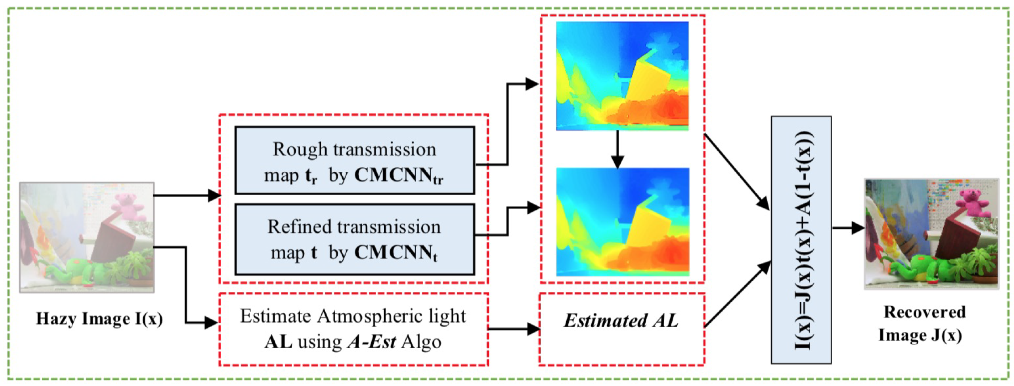
In this section, we present our proposed image dehazing system overcoming the inherent limitations of existing dehazing methods, aiming to improve the method’s efficiency, the accuracy of the estimation of both transmission map and atmospheric light, and the quality of recovered results. Figure 2 illustrates the general process of the proposed method.
The proposed approach has four key components: (1) atmospheric light estimation; (2) transmission map calculation; (3) transmission map refinement; and (4) image reconstruction via the degradation model in Equation (1). For the atmospheric light estimation, we propose a new algorithm based on both image blurriness. Both transmission map and its refined map are generated by a cascaded multi-scale CNN model as two subnetworks (CMCNN and CMCNN). The details of each step are explained in detail in the following subsections.
3.1. Atmospheric Light Estimation
In previous dehazing works, most researchers [20,26,28] set the atmospheric light value empirically (a constant value) or estimate it under the assumption of bright pixels within a local patch. However, the brightest pixel can represent a white object, a gray object in the scene, or an extra-light source, which leads to serious estimation errors. Despite the improvements done in several proposed works [35,36], the estimation of the atmospheric light still has significant errors in specific cases (hazy nighttime images).
To further increase the accuracy of atmospheric light value estimation, we propose a new effective algorithm labeled ‘A-Est’, to avoid the limitations of most previously proposed dehazing methods. This algorithm employs image blur to estimate the atmospheric light value A accurately. This idea is inspired by the fact that haze is one of the main reasons for producing blurred images.
Generally, the atmospheric light value of hazy images is selected as the distant scene points with high intensity. In contrast, far scene points belong to the most blurred image region because the blur amount that occurs on the hazy image increases with scene depth. More clearly, whenever the scene depth increases, the blur amount increases as well. Hence, it is necessary to consider the blur amount in the atmospheric light estimation.
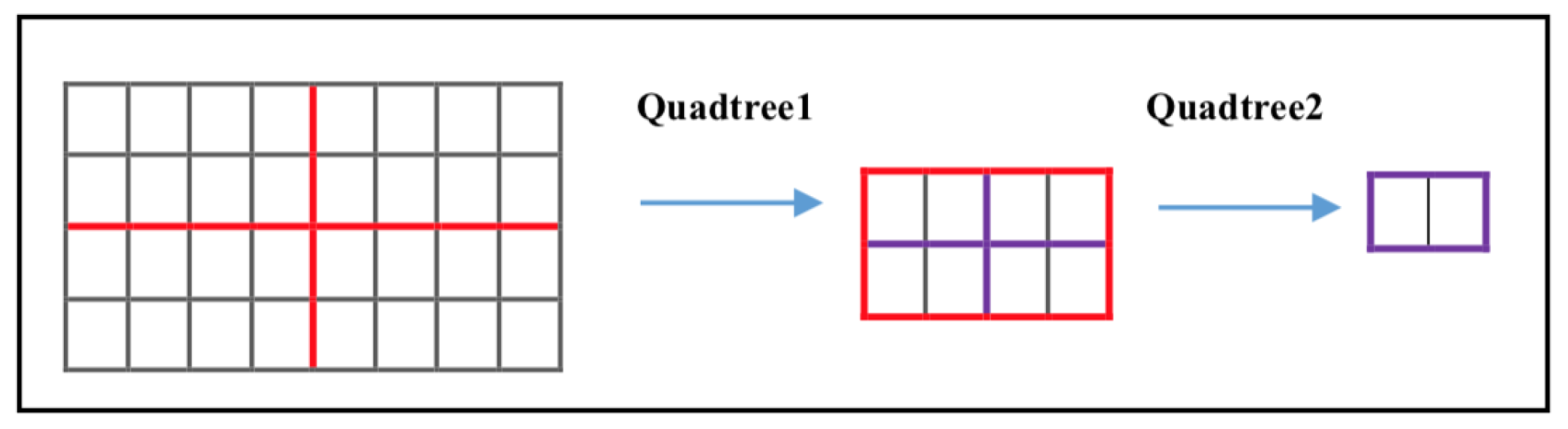
Algorithm 1 explains the running of proposed approach in detail. We utilize a recursive quadtree decomposition (Figure 3 gives an overview) according to the blur amount measured on each quadtree to reduce the solution space of estimated AL value. First, we find the most blurry region in the hazy image by averaging the blur map calculated, and then pick of pixels from this region. Note that Avg operator indicates the average operator.
| Algorithm 1 A-Est |
|
For measuring blur amount on an image, various techniques have been proposed in the literature. Usman et al. [37] discussed and evaluated more than thirty blur measure operators. They showed that “Gradient Energy” is one of the best operators in terms of measure and precision; thus, we choose it to estimate the initial blur map. The Gradient Energy-based blur map can be expressed as:
where = and = . Note that the blur amount can be estimated for the whole hazy image or a sliding window or single pixels.
For hazy images, the atmospheric light AL is defined as a mixture of haze with incident light, and its value A ranges between 0 and 1. According to Equation (1), by setting (A = 0) and (A = 1), the restored scene radiance can be deduced as:
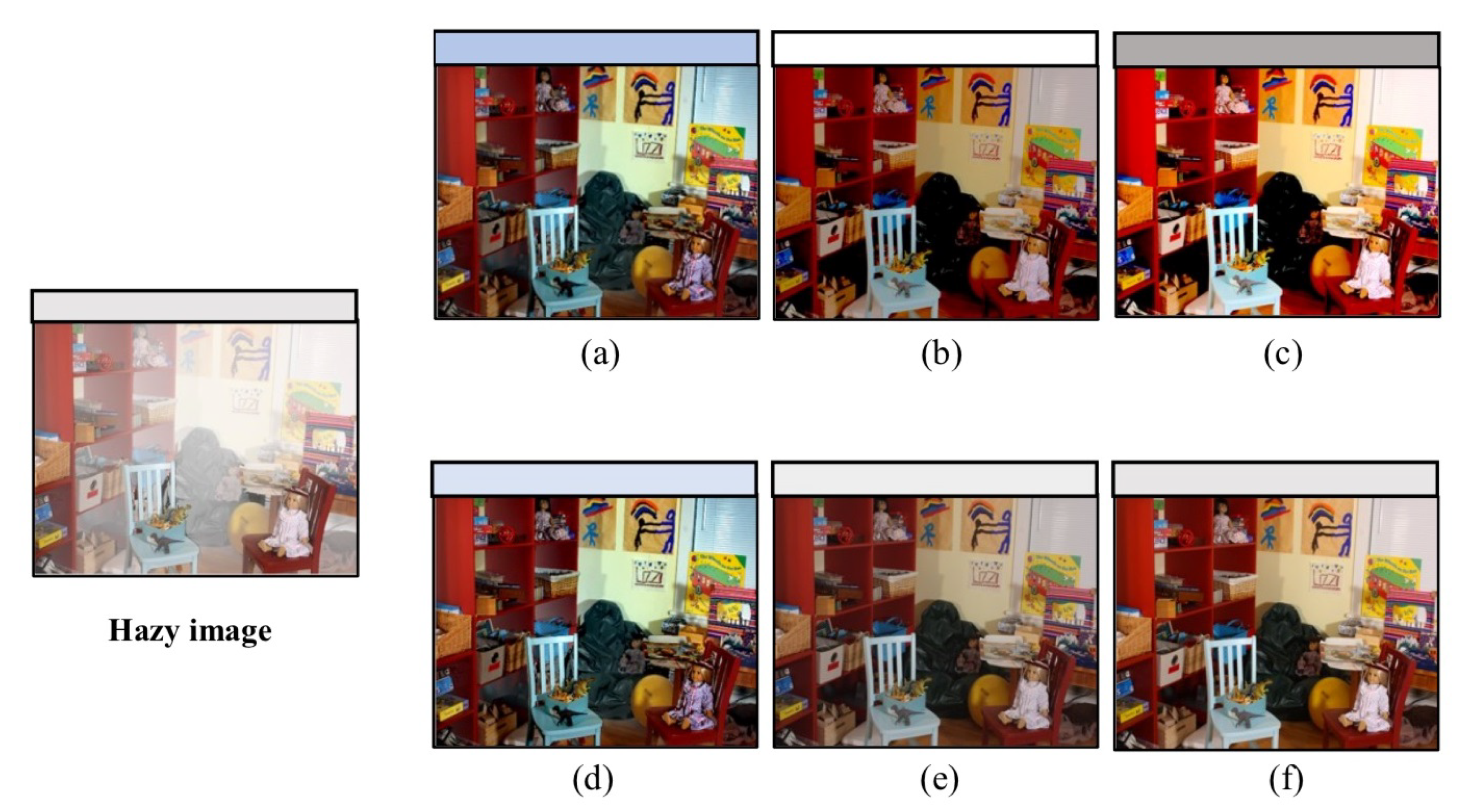
Equation (4) and Figure 4 indicates that recovering a hazy image with poor light A would produce a bright scene radiance (see Figure 6c), while obtaining the opposite result in the case of a bright light A (as shown in Figure 6b). Thus, the accuracy of atmospheric light value estimation is an essential sub-task in image dehazing operation. To assess the performance of “A-Est” algorithm, we present a visual comparison with existing dehazing methods. Table 1 and Figure 5 summarize the AL estimation principle used in each of the concerned methods. The visual comparison employs the physical degradation model in Equation (1), where the transmission map is generated by using the conventional DCP approach [14].
As shown in Figure 6f, the proposed algorithm estimates the AL value accurately from a hazy image, where it achieves an estimation result similar to the ground truth. Some color distortions appear on dehazing results when using Zhu’s [20] and Salazar-Colores’s [35] methods (as shown in Figure 6a,d, the white color of the window becomes blue), which is caused by the inaccuracy of AL estimation. In addition, Cai’s method [28] provides a dim scene radiance, because the estimated A is brighter than that of ground truth (A = 1). Conversely, Sulami’s method [38] produces a bright scene radiance since the estimated A is darker than that of the ground truth. On the other hand, we observe that Haouassi’s method provides an estimation of AL somewhat similar to the ground truth.
3.2. Transmission Medium Estimation Based on Cascaded Multi-scale CNN
For single image dehazing, estimating the transmission medium is an important task, because it is a crucial part according to the hazy image degradation model in Equation (1). Recently, a multitude of strategies has been developed to generate the transmission map from a hazy image directly. In [14], He et al. proposed handcrafted haze-relevant features called Dark Channel under an assumption on haze-free outdoor images. This assumption states that, for haze-free outdoor images, most of the patches have at least one color channel intensity value close to zero for some pixels, except for the sky area patches. Based on this property, the initial dark channel can be expressed as follows:
where c represents a color channel, of RGB image. is a local patch centered at pixel x. This prior has a high relation with the thickness of haze in the image so that the transmission medium can be calculated directly as: .
Subsequently, to estimate the thickness of haze in a hazy image, Zhu et al. [20] built a new color attenuation model that employs saturation and brightness, because, whenever the haze concentration is increased, the saturation is decreased. Based on this model, the haze concentration can be estimated as:
Note that and are two image components in HSV color space (Saturation and Value, respectively). As C(x) is relative to scene depth d, the transmission medium can be calculated directly using Equation (2).
Despite the great success achieved by these haze-relevant feature-based dehazing methods for removing haze from single images, they can be invalid in particular cases. He’s method becomes useless for the sky region in the hazy image, and Zhu’s model fails to remove haze effectively in the case of thick haze. Differently, inspired by the inherent high performance of CNNs, we propose a two-stage cascaded multi-scale CNN architecture to generate accurate transmission maps for hazy images.
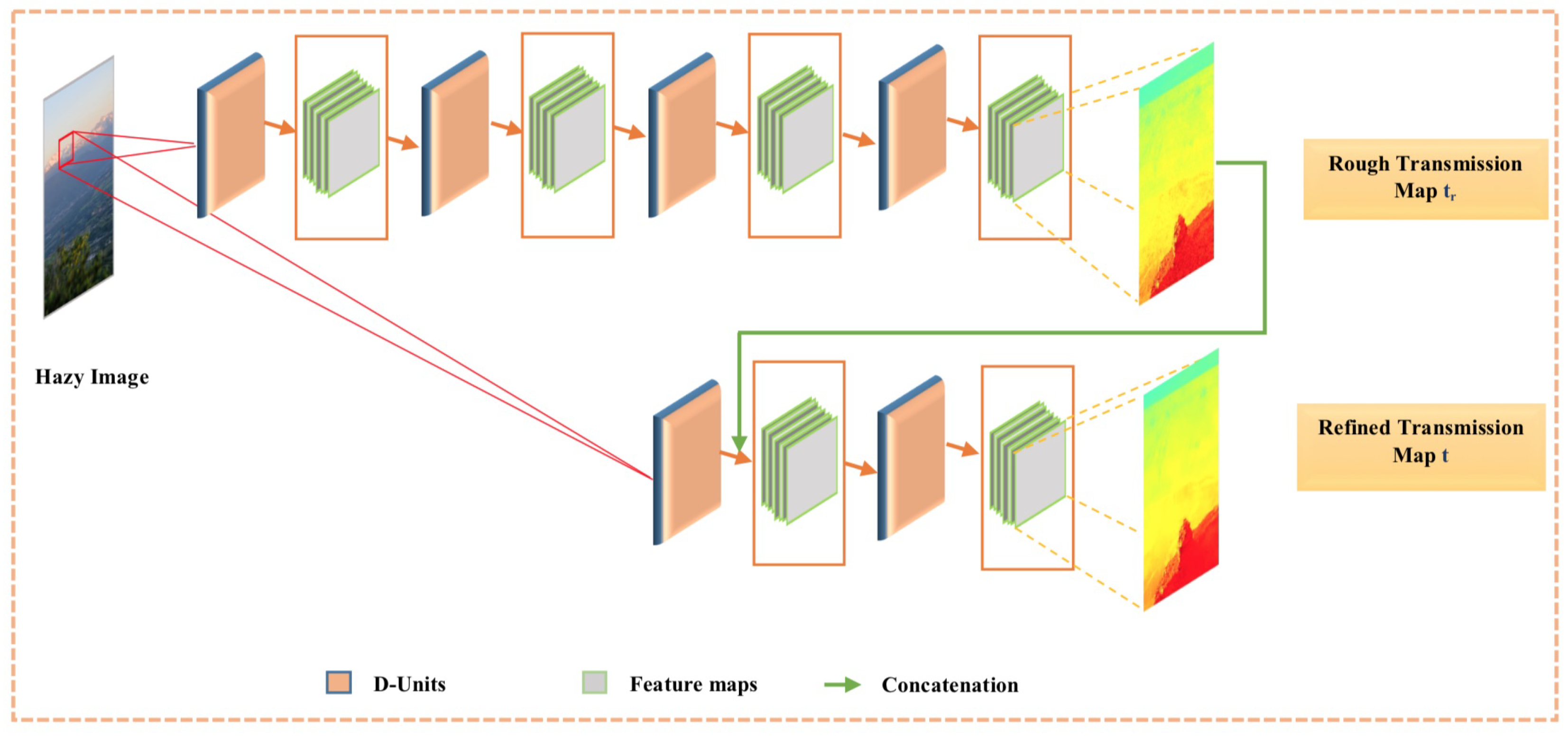
Figure 7 illustrates the general mechanism of the proposed cascaded multi-scale CNN for generating transmission maps for hazy images. The proposed cascaded architecture consists of two subnetworks (CMCNN and CMCNN), one for producing rough transmission maps and the other for refined transmission maps t.
3.2.1. Rough Transmission Map Subnetwork CMCNN
CMCNN is composed of four sequential cascaded MCNN D-units. Each D-unit is defined as follow:
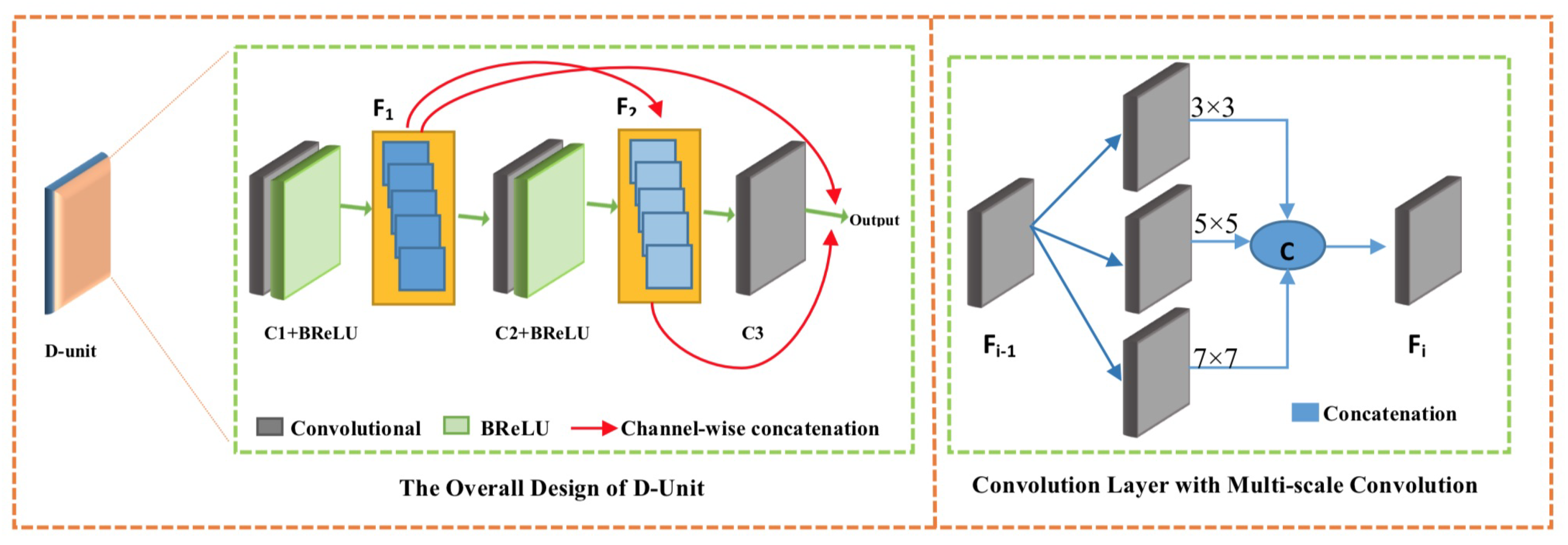
- D-Unit Structure: The overall design of a D-unit is shown in Figure 8 (Left) and comprises three multi-scale convolutional layers pursued by a Bilateral Rectified Linear Unit (BReLU) [28], except for the last convolutional layer. Each convolutional layer represents a fusion of convolutions with a different kernel size (, , and ), thus it is called multi-scale convolution. Regarding the number of filters , for the first and second layers and , we use 16 filters, and for the last layer we use eight filters.The idea of these D-units is inspired by the DenseNet [39] architecture, where layers of each D-unit are densely connected. The output feature maps of each layer are concatenated with those of all succeeding layers; feature maps of the first layer are concatenated with that of the second and third layers and . Moreover, the same for feature maps of are concatenated with feature maps.The proposed D-units-based architecture has significant benefits, e.g. it can avoid the gradient vanishing problem that deep CNNs have with fewer required parameters. In addition, it can maximize the information flow with non-redundancy of feature maps.
- Multi-scale CNN: It is a general truth that human visual perception is a multi-scale neural system. In contrast, using CNN models to solve low-level computer vision tasks always requires the best choice of kernel size. The small size of the filter window can highlight only low-frequency features and neglect the high-frequency content or other important information. Likewise, big kernels can extract only high-frequency details and disregard low-frequency image information. Besides, employing CNNs with successive single filter sizes produces a deeper CNN architecture, which makes the computations complicated and thus hinders the speed of the training process. Therefore, the success of multi-scale CNN representation [26,28] motivates us to apply multi-scale CNN layers in our work to obtain both low- and high-frequency details. In this work, each convolutional layer can be defined as a concatenation of three convolutions with different filter sizes (, , and ), as shown in Figure 8 (right), and can be expressed as:where represents the i-th layer generated feature maps, n is the layer depth (n = 3), and are the output feature maps attained by the three convolutions (, , and ) in each multi-scale CNN layer.
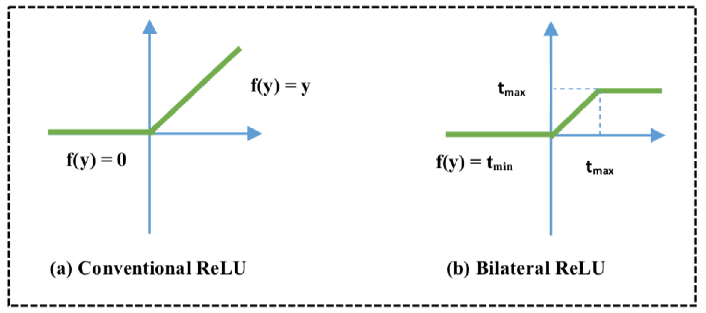
- BReLU: Recently, most of the deep learning methods [26,40] have employed the ReLU as a nonlinear transfer function to solve the problem of vanishing gradient instead of the previous weak sigmoid function [41] that makes the learning convergence very slow. However, the ReLU function [42] is especially designed for classification problems. In this work, we adopt the BReLU function: Cai [28] proposed a sparse representation, benefiting from local linearity of ReLU and preserving the bilateral control of Sigmoid function and considering the restoration problem. Figure 9 shows the difference between the conventional ReLU and Bilateral ReLU; note that =0 and .
- Concatenation: After generating the rough transmission map through CMCNN subnetwork, it is transferred to CMCNN subnetwork as support information, where it is merged with the feature maps extracted by the first unit to explore new features. Exploring new features by using concatenation augments the performance of the CMCNN to predict efficient refined transmission maps.
3.2.2. Refined Transmission Map via CMCNN Subnetwork
The subnetwork CMCNN is offered to settle the problem of the blocking artifacts that appear on the edges of the estimated rough transmission map. The structure of CMCNN is similar to that of CMCNN, except for the number of used units. CMCNN (shown in Figure 7) consists of three D-units that extract features from input hazy image and fed from the rough transmission map, by combining it with image features produced by the first unit. Note that the internal structure of convolutional layers is also similar to that of CMCNN subnetwork with a different filter size N = 8.
3.2.3. Training of CMT
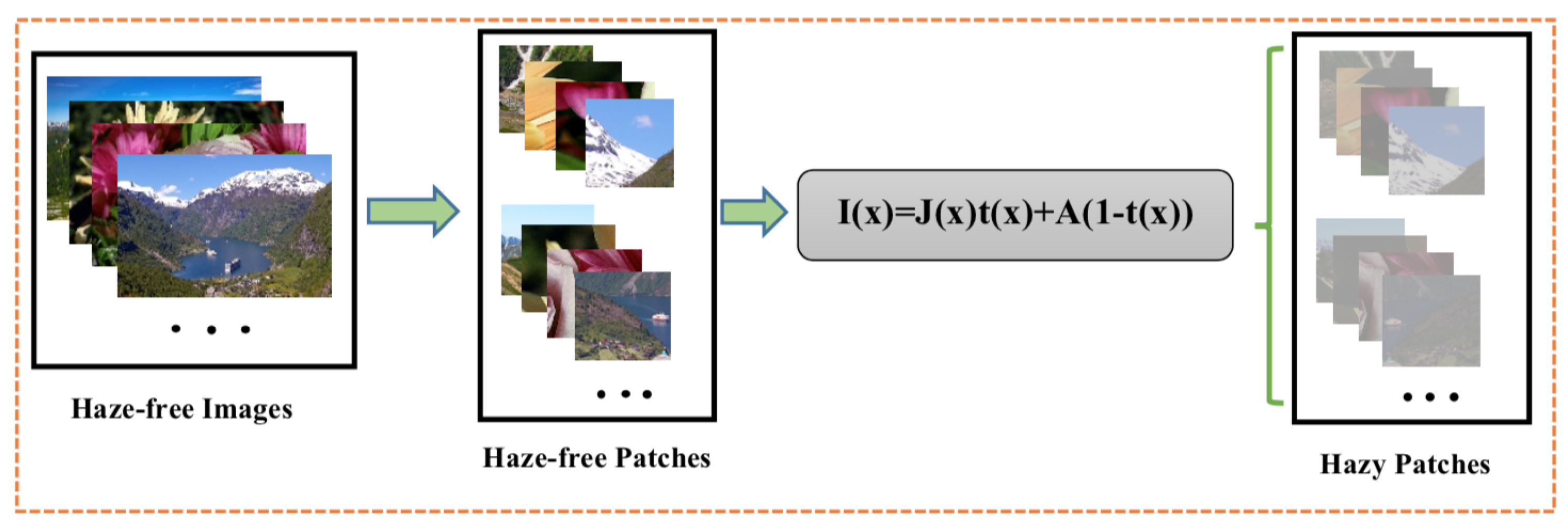
- Training Data: A well-performed network cannot be attained only by making a network with good structure and perfect implementation, but it is also based on the training process. Generally, deep learning networks are data-hungry models. However, it is not easy to provide massive data to train the network, especially for providing pairs of real-world hazy images and their truth transmission maps. Based on the assumption that indicates that the transmission map of an image is constant in small patches, and employing the hazy image formation model (Equation (1), by regarding A = 1), we synthesized a massive number of hazy/clear pairs of patches (as shown in Figure 10). First, we collected from the Internet more than 1000 natural clear images for different scenes (mountain, herb, water, clouds, and traffic). Then, we randomly picked 10 patches of from each image, thus totally we had 10,000 training patches.To reduce the overfitting and make the training process more robust, We added a GaussianNoise layer as the input layer. The amount of noise must be small. Given that the input values are within the range [0, 1], we added Gaussian noise with a mean of 0.0 and a standard deviation of 0.01, chosen arbitrarily.
- Training Strategy and Network Loss: The prediction of the transmission map requires the mapping link between the color image and its corresponding transmission medium through automatic supervised learning. The optimization of the model is realized by minimizing the loss function between I(x) and its truth transmission, with predicting optimal parameters (weights and biases). First, the network feeds on the training image patches I(x) and updates the parameters iteratively, until the loss function reaches the minimum value. The loss function in learning models is a crucial part because it measures the performance of the model to predict the desired result.The extensively used loss function in image dehazing is MSE (Mean Squared Error) that can be expressed as follows:where represents the predicted transmission medium, is the truth transmission medium, and M is the number of hazy image patches in the training data.As noticed, although the loss can maintain both edges and details well during the reconstruction process, it cannot preserve sufficiently the background texture. Therefore, we also consider the SSIM loss [43] in this work to assess the texture and structure similarity. The structural similarity (SSIM) value of each pixel x can be calculated as follows:Note that and are constants of regularization set as default 0.02 and 0.03. , , and represent the average and standard deviation of the predicted image patch x and ground truth image patch y, respectively. Eventually, the loss is calculated as:For the proposed network CMT, the final loss is defined as the aggregation of and as follows:
4. Experimental Results
4.1. Network Implementation
As an optimization training method, we employed the ADAM optimizer [44] to update network parameters iteratively, using the conventional learning rate 0.001, with hyper-parameters and . The implementation of the MSCDnet was done using TensorFlow framework on a PC of Intel® Core i7-7700 @ 3.60 Hz CPU and a Nvidia GTX 1080 Ti GPU.
4.2. Network Parameters
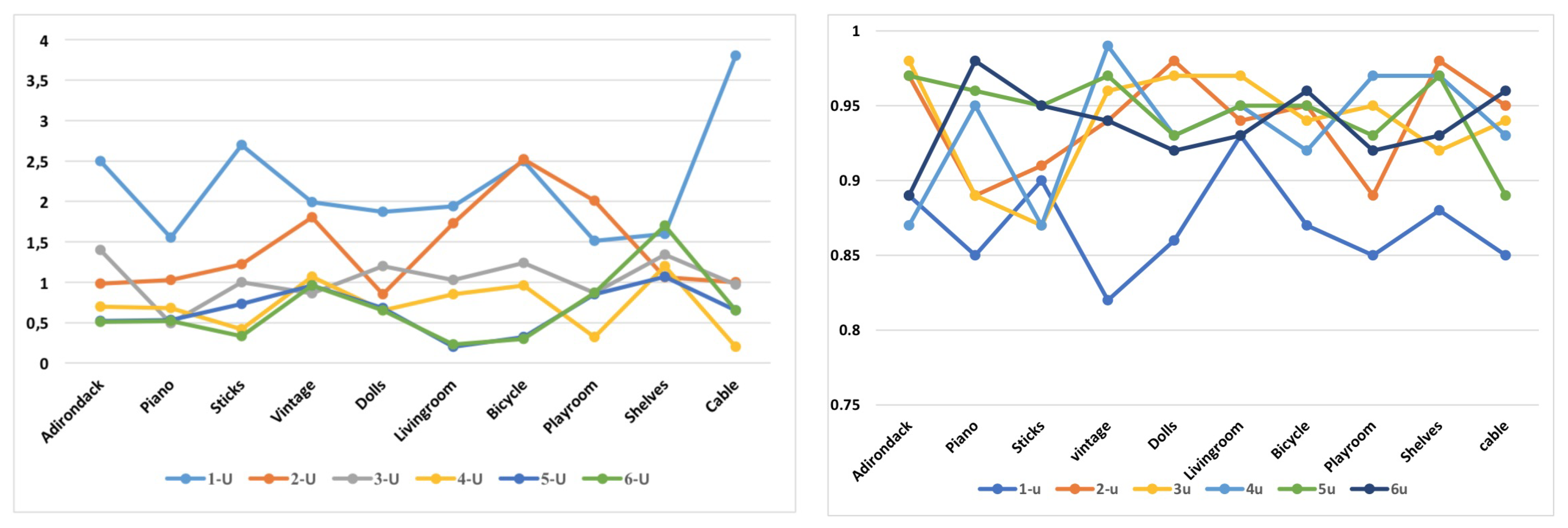
As shown above, our proposed model consists of D-units (four for rough transmission map and two for refined transmission map). The choice of number of D-units was investigated through an experimental comparison in terms of number of D-units and quality loss results, as summarized in Table 2.
4.3. Haze Removal
As mentioned above, pivotal estimates (transmission map t and ) of dehazing system were calculated through a high-performance strategy. Consequently, haze removal operation can be attained easily by employing the atmospheric degradation model in Equation (1) as:
where and represent recovered image and hazy image, respectively. and are the estimated transmission map and , respectively. Figure 12 shows the practical results achieved by the proposed dehazing system.
4.4. Evaluation of Proposed Method
To prove the performance of our proposed dehazing method, we show in this section a detailed comparison with one powerful dehazing assumption, DCP [14], and four recently proposed haze removal methods, including three learning-based methods: Cai [28], Ren [26], Li [40], and Salazar-Colores [35]. Figure 13, Figure 14 and Figure 15 show some examples of haze removal results of these methods, including ours. For an efficient evaluation, the proposed method was tested on three different hazy images datasets that are publicly available, namely FRIDA [45], D-HAZY (Middlebury) [46], and RESIDE (SOTS) [47], and a set of hazy images that were generated by us.
We carried out quantitative and qualitative comparisons analysis on hazy real-world and synthetic images, as detailed in the next subsections. The comparative examples shown in figures are named as room, cable, jade, teddy, river, park, street, mountain1, tree, forest, and mountain2.
4.4.1. Qualitative Comparison on Synthetic and Real-world Hazy Images
For qualitative comparison analysis, we present several examples of dehazing results for methods mentioned above [14,26,28,35,40]. Figure 13, Figure 14 and Figure 15 show some results on both indoor and outdoor hazy synthetic images and real-world outdoor hazy images, respectively.
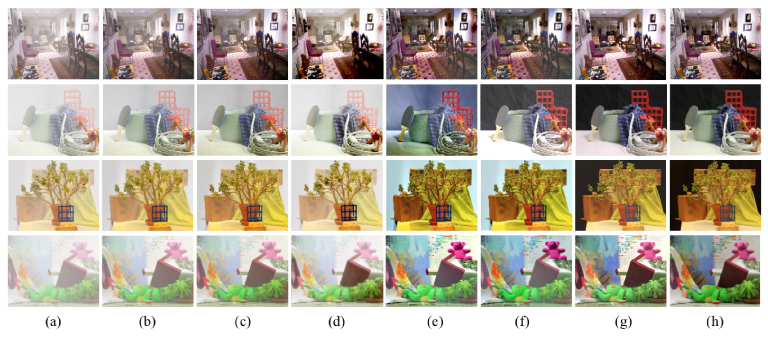
- Comparison on synthetic images: As shown in Figure 13g and Figure 14g, the proposed method has a good performance on hazy synthetic images, where it is not easy to discern our results from the truth images. It achieved good dehazing results, considering haze-removing, color-preserving, visibility-enhancing, and edge-preserving. By contrast, we observe that He et al.’s [14] and Ren et al.’s [26] results still contain a thin haze layer in most synthetic images, especially for thick haze. Thus, these methods are sensitive to the thickness of haze. Cai et al.’s [24] method could lessen haze on images, but it left some haze trace on distant scene objects (e.g., room, teddy, and mountain2 images). On the other hand, Li et al.’s [40] and Salazar-Colores et al.’s [35] methods could remove haze from synthetic images successfully. However, these two methods have a color-shift problem in some regions (e.g., the background of cable image and sky color in park image).
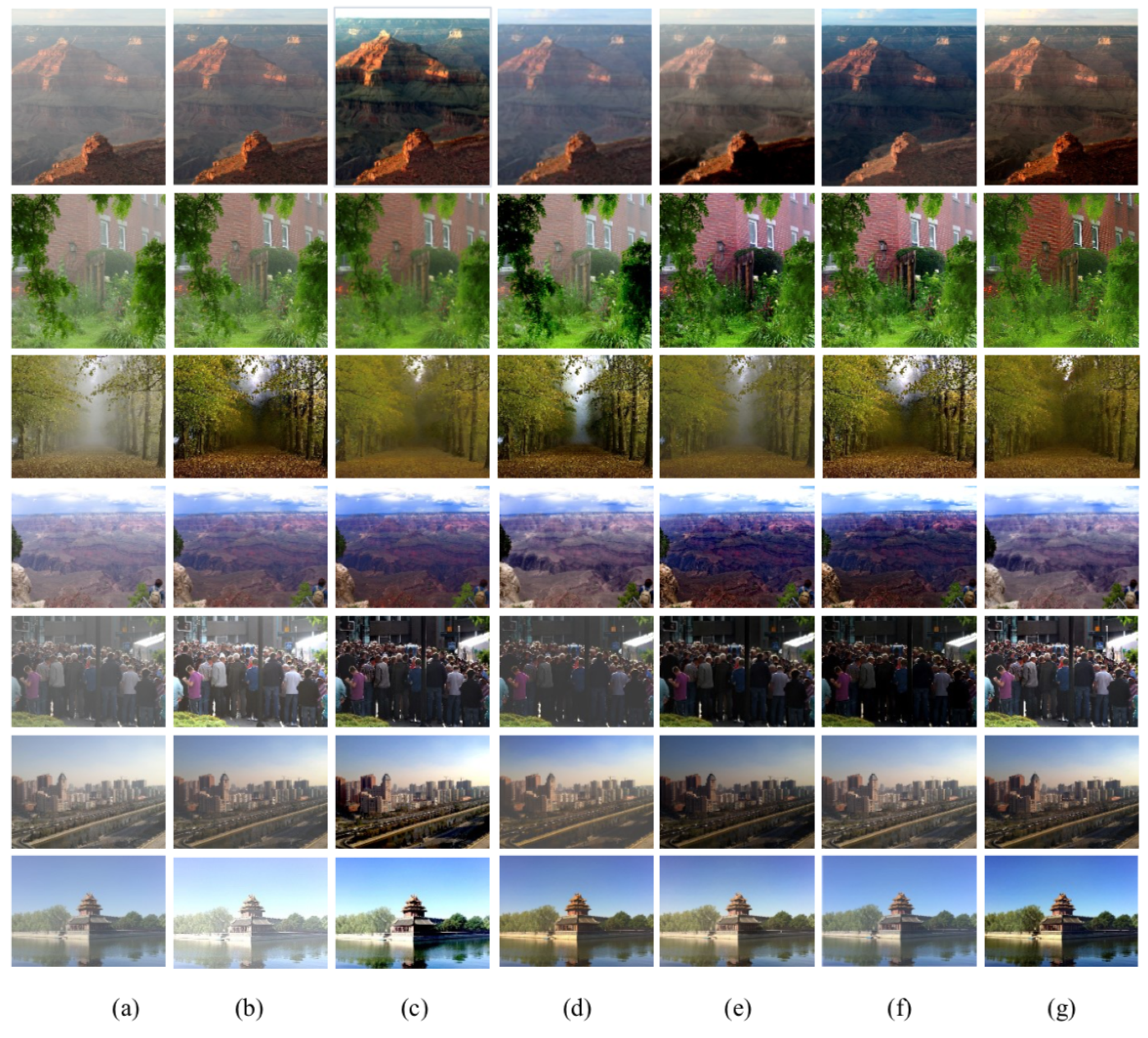
- Comparison on real-world images: In this part, we performed comparisons on the real-world hazy images. The real-world hazy images were collected from the Internet because of the unavailability of a hazy images dataset. Figure 15 demonstrates examples of comparisons on real-world images with comparative methods [14,26,28,35,40].At first glance, we can say that most methods removed haze from images effectively. However, if inspecting carefully, we can discover that He et al.’s [14] method still has some residual haze in specific regions (e.g., tree and forest images). Although the other comparative methods [26,28,35,40] could eliminate haze particles from images efficiently, the over-enhancement problem invades most of the results (e.g., forest, mountain1, and tree images); in addition, these methods generate artificial colors on sky region (mountain1 image). Besides, Cai et al.’s [28] and Li et al.’s [40] results contain halo artifacts caused by edge-deformation. By contrast, our proposed method yielded promising results on real-world images, where it could eliminate haze, produce real vivid colors, and preserve edges of recovered images.
4.4.2. Quantitative Comparison Analysis
To validate the qualitative comparison above-discussed, we present here a quantitative comparison to assess and rank our proposed dehazing system. In this comparison, we employed two extensively used FR-IQA metrics, namely SSIM and MSE. SSIM is used to measure the similarity between the restored image and its ground-truth image, while MSE is used to calculate the error between them. Since SSIM and MSE are quality measures that need a reference image, they are limited to synthetic images only because the ground truths of these images are available.
Furthermore, we measured the accuracy of the restored images on synthetic images by exploiting some common NR-IQA (FADE [48], e, and ). The indexes e and are two contrast enhancement indicators presented by Hautiere et al. [49], which measure the ability to recover the invisible edges and the quality of the contrast enhancement, respectively. FADE indicator evaluates the ability to remove haze from hazy images. Table 3 sums up the average scores of SSIM, MSE, e, , FADE, and running time (T) of the comparative methods as well as ours.
The high score of SSIM implies a high similarity between the ground-truth and the recovered image. A low value of FADE designates a high ability for removing haze. Whenever the values of e and are high, the visibility of the restored images is enhanced. The best values of each indicator are written in bold.
As evident from the results in Table 3, among all the comparative methods, our proposed model achieved the best scores of SSIM, MSE, and FADE, and ranked the second in term of visibility enhancement. In addition, it achieved the lowest running time when compared to other comparative methods (T = 0.386). This significant outcome implies that the proposed method can tackle the problem of haze removing, noise suppressing, and visibility-enhancing of recovered images, effectively.
Moreover, Table 3 shows that FADE indicator values obtained by He et al. [14] and Ren et al. [26] are a little bit high, which means that their results still have some haze residue. In addition, we can see that Salazar-Colores et al. [35] attained the best score of indicator, which comes from the over-enhancement, as discussed in the qualitative comparison. He et al.’s method [14] has a high time complexity (T = 14.901), far from all comparative methods, because of the soft-matting filter. This analysis confirms that the quantitative evaluation validates the previously-discussed qualitative analysis.
Moreover, we applied the NR-IQA metrics on real-world hazy images to quantify the performance of the proposed system. To assess the performance quantitatively, we collected from the Internet more than 500 real-world hazy images of average size 640 × 480. Table 4 summarizes the average scores of e, , FADE, and running time (T) on real-world hazy images of the comparative methods, including our proposed method.
As it is visible from the results in Table 4, the proposed system performed quickly compared to other methods and achieved an average of 0.453 s, while He et al.’s [14] method obtained an average of 16.033 s, because of the complexity of soft-matting filter refinement. In addition, He’s method attained the highest score of FADE indicator, which indicates that this method fails to remove haze from the input hazy image, and the second highest score was attained by Ren’s method, as noticed also from the results in Figure 15. In contrast, our proposed system had the lowest FADE score, which states that the proposed method can remove haze efficiently, and attain a good visibility enhancement according to and e values. while Li et al. [40], Salazar-Colores et al. [35], and Cai et al. [28] attained a considerable visibility enhancement according to and e values.
4.4.3. Visual Results on Nighttime Hazy Images
As proved in previous sections, our proposed system shows good performance of dehazing on both synthetic and real-world hazy images, where it achieves good quality results in terms of haze removability and quality enhancement. Furthermore, as mentioned above, the proposed method performs well on nighttime hazy images. Figure 16 shows some visual results on nighttime images compared with some previously proposed dehazing methods by He et al. [14], Cai et al. [28], and Ren et al. [26].
As shown in Figure 16e, it is obvious that the proposed system can remove the haze on the input nighttime hazy images and recover the real color and appearance. By contrast, the results achieved by He et al. [14], Cai et al. [28], and Ren et al. [26] still suffer from haze particles (see train image results) and real color distortions (see the sky in Ren’s Figure 16d results for the second and third images).
5. Discussion
According to the previous analysis, the proposed method outperforms most of the state-of-the-art dehazing approaches, in terms of haze-removal, visibility-enhancing, and edge-preserving, where it can overcome most of the shortcomings of those methods. This outstanding success emphasizes the robustness and effectiveness of both and transmission medium estimation strategies (“A-Est” algorithm and CMT model), which affirms that the proposed AL estimation algorithm can calculate the atmospheric light accurately, and theproposed architecture CMT estimates the haze thickness efficiently. These are the advantages of our proposed method.
Even though the proposed CMT is based on synthetic images training, the dehazing results prove that the proposed architecture can handle real-world images as well.
6. Conclusions
This paper proposes a haze removal system that considers both atmospheric light and transmission maps and avoids the shortcomings of most state-of-the-art approaches. The proposed system comprises two essential parts, a simple AL estimation algorithm called “A-Est” that considers image blurriness and an efficient transmission map estimator based on a cascaded multi-scale CNN architecture. This architecture has two sub-tasks, one for generating a rough transmission (CMCNN) map and the other to refine it (CMCNN). Although the proposed model is learned using hazy synthetic images, it can handle real-world hazy images effectively as well. Experimental results demonstrate that the proposed system estimated AL and t accurately, producing high-quality promising dehazing outcomes that are free from haze, without distorted colors, and improved contrast visibility. As future work, we will carry on with improving the proposed model, where we will integrate the atmospheric light estimation in it to further increase the speed of the dehazing system.
Author Contributions
Conceptualization, S.H.; Formal analysis, S.H., and D.W.; Funding acquisition, D.W.; Investigation, S.H.; Methodology, S.H.; Project administration, D.W.; Software, S.H. and D.W.; Supervision, D.W.; Validation, D.W.; Writing—original draft, S.H.; and Writing—review and editing, S.H. and D.W. All authors have read and agreed to the published version of the manuscript.
Funding
The work presented in this paper was supported by the National Natural Science Foundation of China under Grant no. 61370201.
Conflicts of Interest
The authors declare no conflict of interest.
Abbreviations
The following abbreviations are used in this manuscript:
| MCNN | Multi-scale Convolutional Neural Network |
| CMCNN | Cascaded Multi-scale Convolutional Neural Network |
| BReLu | Bilateral Rectified Linear Unit |
| CMT | Cascaded Multi-scale Network for Transmission map Estimation |
| MRF | Markov Random Field |
| ICA | Independent Component Analysis |
| DCP | Dark Channel Prior |
| CNN | Convolutional Neural Network |
| DNN | Deep Neural Network |
| FR-IQA | Full Reference Image Quality Assessment |
| NR-IQA | No Reference Image Quality Assessment |
References
- Zeng, L.; Yan, B.; Wang, W. Contrast Enhancement Method Based on Gray and Its Distance Double-Weighting Histogram Equalization for 3D CT Images of PCBs. Math. Probl. Eng. 2016, 2016, 1529782. [Google Scholar] [CrossRef]
- Chin, Y.W.; Shilong, L.; San, C.L. Image contrast enhancement using histogram equalization with maximum intensity coverage. J. Mod. Opt. 2016, 63. [Google Scholar] [CrossRef]
- Zhou, L.; Bi, D.Y.; He, L.Y. Variational Histogram Equalization for Single Color Image Defogging. Math. Probl. Eng. 2016. [Google Scholar] [CrossRef]
- Dong, H.; Li, D.; Wang, X. Automatic Restoration Method Based on a Single Foggy Image. J. Image Graph. 2012. [Google Scholar] [CrossRef]
- Zhou, J.; Zhou, F. Single image dehazing motivated by Retinex theory. In Proceedings of the 2nd International Symposium on Instrumentation and Measurement, Sensor Network and Automation (IMSNA), Toronto, ON, Canada, 23–24 December 2013; pp. 243–247. [Google Scholar] [CrossRef]
- Fang, S.; Xia, X.; Huo, X.; Chen, C. Image dehazing using polarization effects of objects and airlight. Opt. Soc. Am. 2014. [Google Scholar] [CrossRef] [PubMed]
- Schechner, Y.Y.; Narasimhan, S.G.; Nayar, S.K. Polarization-Based Vision through Haze. Appl. Opt. 2003, 42, 511–525. [Google Scholar] [CrossRef]
- Schechner, Y.Y.; Narasimhan, S.G.; Nayar, S.K. Blind Haze Separation. In Proceedings of the IEEE Computer Society Conference on Computer Vision and Pattern Recognition CVPR, New York, NY, USA, 17–22 June 2006. [Google Scholar]
- Narasimhan, S.G.; Nayar, S.K. Chromatic Framework for Vision in Bad Weather. In Proceedings of the IEEE Conference on Computer Vision and Pattern Recognition CVPR, Hilton Head Island, SC, USA, 15 June 2000. [Google Scholar]
- Narasimhan, S.G.; Nayar, S.K. Contrast Restoration of Weather Degraded Images. IEEE Trans. Pattern Anal. Mach. Intell. 2003, 25, 713–724. [Google Scholar] [CrossRef] [Green Version]
- Nayar, S.K.; Narasimhan, S.G. Vision in Bad Weather. In Proceedings of the IIEEE International Conference on Computer Vision, Kerkyra, Greece, 20–27 September 1999. [Google Scholar]
- Tan, R.T. Visibility in Bad Weather from a Single Image. In Proceedings of the IEEE International Conference on Computer Vision and Pattern Recognition, Anchorage, AK, USA, 23–28 June 2008. [Google Scholar]
- Fattal, R. Single Image Dehazing. In Proceedings of the ACM SIGGRAPH, Los Angeles, CA, USA, 11–15 August 2008. [Google Scholar]
- He, K.; Sun, J.; Tang, X. Single Image Haze Removal Using Dark Channel Prior. IEEE Trans. Pattern Anal. Mach. Intell. 2011, 33, 2341–2353. [Google Scholar]
- Lin, Z.; Wang, X. Dehazing for Image and Video Using Guided Filter. Appl. Sci. 2012, 2, 123–127. [Google Scholar] [CrossRef]
- Xu, H.; Guo, J.; Liu, Q.; Ye, L. Fast Image Dehazing Using Improved Dark Channel Prior. In Proceedings of the IEEE International Conference on Information Science and Technology, Hubei, China, 23–25 March 2012; pp. 663–667. [Google Scholar] [CrossRef]
- Song, Y.; Luo, H.; Hui, B.; Chang, Z. An Improved Image Dehazing and Enhancing Method Using Dark Channel Prior. In Proceedings of the 27th Chinese Control and Decision Conference, Qingdao, China, 23–25 May 2015; pp. 5840–5845. [Google Scholar] [CrossRef]
- Yuan, X.; Ju, M.; Gu, Z.; Wang, S. An Effective and Robust Single Image Dehazing Method Using the Dark Channel Prior. Information 2017, 8, 57. [Google Scholar] [CrossRef] [Green Version]
- Hsieh, C.; Zhao, Q.; Cheng, W. Single Image Haze Removal Using Weak Dark Channel Prior. In Proceedings of the 9th International Conference on Awareness Science and Technology (iCAST), Fukuoka, Japan, 19–21 September 2018; pp. 214–219. [Google Scholar] [CrossRef]
- Zhu, Q.S.; Mai, J.M.; Shao, L.A. Fast Single Image Haze Removal Algorithm Using Color Attenuation Prior. IEEE Trans. Image Process. 2015, 24, 3522–3533. [Google Scholar] [PubMed] [Green Version]
- Krizhevsky, A.; Sutskever, I.; Hinton, G.E. Imagenet: Classification with Deep Convolutional Neural Networks. In Proceedings of the Advances in Neural Information Processing Systems, Lake Tahoe, NV, USA, 3–6 December 2012; pp. 1097–1105. [Google Scholar]
- Long, J.; Shelhamer, E.; Darrell, T. Fully Convolutional Networks for Semantic Segmentation. In Proceedings of the IEEE Conference on Computer Vision and Pattern Recognition, Boston, MA, USA, 7–12 June 2015. [Google Scholar]
- Fu, M.; Wu, W.; Hong, X.; Liu, Q.; Jiang, J.; Ou, Y.; Zhao, Y.; Gong, X. Hierarchical Combinatorial Deep Learning Architecture for Pancreas Segmentation of Medical Computed Tomography Cancer Images. BMC Syst. Biol. 2018, 12, 56. [Google Scholar] [CrossRef] [Green Version]
- Erhan, D.; Szegedy, C.; Toshev, A.; Anguelov, D. Scalable Object Detection Using Deep Neural Networks. In Proceedings of the EEE Conference on Computer Vision and Pattern Recognition, Columbus, OH, USA, 23–28 June 2014; pp. 2155–2162. [Google Scholar]
- Xie, J.; Xu, L.; Chen, E. Image Denoising and Inpainting with Deep Neural Networks. In Proceedings of the Advances in Neural Information Processing Systems, Lake Tahoe, NV, USA, 3–6 December 2012; pp. 341–349. [Google Scholar]
- Ren, W.; Liu, S.; Zhang, H.; Pan, J.; Cao, X.; Yang, M.H. Single Image Dehazing via Multi-scale Convolutional Neural Networks. In Proceedings of the European Conference on Computer Vision, Amsterdam, The Netherlands, 8–16 October 2016. [Google Scholar]
- Rashid, H.; Zafar, N.; Iqbal, M.J.; Dawood, H.; Dawood, H. Single Image Dehazing using CNN. In Proceedings of the International Conference on Identification, Information and Knowledge in the Internet of Things, IIKI 2018, Beijing, China, 19–21 October 2019; Volume 147, pp. 124–130. [Google Scholar]
- Cai, B.; Xu, X.; Jia, K.; Qing, C.; Tao, D. DehazeNet: An End-to-End System for Single Image Haze Removal. IEEE Trans. Image Process. 2016, 25, 5187–5198. [Google Scholar] [CrossRef] [PubMed] [Green Version]
- Song, Y.; Li, J.; Wang, X.; Chen, X. Single Image Dehazing Using Ranking Convolutional Neural Network. IEEE Trans. Multimed. 2018, 20, 1548–1560. [Google Scholar] [CrossRef] [Green Version]
- Li, C.; Guo, J.; Porikli, F.; Guo, C.; Fu, H.; Li, X. DR-Net: Transmission Steered Single Image Dehazing Network with Weakly Supervised Refinement. arXiv 2017, arXiv:1712.00621v1. [Google Scholar]
- Narasimhan, S.G.; Nayar, S.K. Removing Weather Effects from Monochrome Images. In Proceedings of the IEEE Computer Society Conference of Computer Vision Pattern Recognition CVPR, Kauai, HI, USA, 8–14 December 2001. [Google Scholar]
- Narasimhan, S.G.; Nayar, S.K. Vision and the Atmosphere. In Proceedings of the ACM SIGGRAPH ASIA 2008 Courses -SIGGRAPH Asia 08, Bhubaneswar, India, 16–19 December 2008. [Google Scholar]
- Hu, Y.; Wang, K.; Zhao, X.; Wang, H.; Li, Y.S. Underwater Image Restoration Based on Convolutional Neural Network. Proc. Mach. Learn. Res. 2018, 95, 296–311. [Google Scholar]
- Tao, L.; Zhu, C.; Song, J.; Lu, T.; Jia, H.; Xie, X. Low-light image enhancement using CNN and bright channel prior. In Proceedings of the IEEE International Conference on Image Processing (ICIP), Beijing, China, 17–20 September 2017; pp. 3215–3219. [Google Scholar]
- Salazar-Colores, S.; Cabal-Yepez, E.; Ramos-Arreguin, J.M.; Botella, G.; Ledesma-Carrillo, L.M.; Ledesma, S. A Fast Image Dehazing Algorithm Using Morphological Reconstruction. IEEE Trans. Image Process. 2019, 28, 2357–2366. [Google Scholar] [CrossRef]
- Haouassi, S.; Wu, D.; Hamidaoui, M.; Tobji, R. An Efficient Image Haze Removal Algorithm Based on New Accurate Depth and Light Estimation Algorithm. Int. J. Adv. Comput. Sci. Appl. 2019, 10, 64–76. [Google Scholar] [CrossRef]
- Ali, U.; Mahmood, M.T. Analysis of Blur Measure Operators for Single Image Blur Segmentation. Appl. Sci. 2018, 8, 807. [Google Scholar] [CrossRef] [Green Version]
- Sulami, M.; Glatzer, I.; Fattal, R.; Werman, M. Automatic recovery of the atmospheric light in hazy images. In Proceedings of the IEEE International Conference Computer Photography, Santa Clara, CA, USA, 2–4 May 2014; pp. 1–11. [Google Scholar]
- Huang, G.; Liu, Z.; Weinberger, K.Q.; van der Matten, L. Densely connected convolutional networks. In Proceedings of the IEEE International Conference on Computer Vision and Pattern Recognition (CVPR), Honolulu, HI, USA, 21–26 July 2017; pp. 2261–2269. [Google Scholar]
- Li, C.; Guo, J.; Porikli, F.; Fu, H.; Pang, Y. A Cascaded Convolutional Neural Network for Single Image Dehazing. IEEE Access 2018, 6, 24877–24887. [Google Scholar] [CrossRef]
- Hinton, G.E.; Salakhutdinov, R.R. Reducing the Dimensionality of Data with Neural Networks. Science 2006, 313, 504–507. [Google Scholar] [CrossRef] [PubMed] [Green Version]
- Nair, V.; Hinton, G.E. Rectified Linear Units Improve Restricted Boltzmann Machines. In Proceedings of the 27th International Conference on Machine Learning (ICML-10), Haifa, Israel, 21–24 June 2010; pp. 807–814. [Google Scholar]
- Wang, Z.; Bovik, A.; Sheikh, H.; Simoncelli, E. Image Quality Assessment: From error visibility to structural similarity. IEEE Trans. Image Process. 2004, 13, 3888–3901. [Google Scholar] [CrossRef] [PubMed] [Green Version]
- Kingma, D.; Ba, J. Adam: A method for stochastic optimization. In Proceedings of the International Conference on Learning Representations (ICLR 2015), San Diego, CA, USA, 7–9 May 2015; pp. 87–95. [Google Scholar]
- Tarel, J.P.; Hautiere, N.; Cord, A.; Gruyer, D.; Halmaoui, H. Improved Visibility of Road Scene Images under Heterogeneous Fog. In Proceedings of the IEEE Intelligent Vehicles Symposium (IV’10), San Diego, CA, USA, 21–24 June 2010. [Google Scholar]
- Scharstein, D.; Hirschmller, H.; Kitajima, Y.; Krathwohl, G.; Nesic, N.; Wang, X.; Westling, P. High-resolution stereo datasets with subpixel-accurate ground truth. In Proceedings of the German Conference on Pattern Recognition, Münster, Germany, 3–5 September 2014. [Google Scholar]
- Li, B.; Ren, W.; Fu, D.; Tao, D.; Feng, D.; Zeng, W.; Wang, Z. Benchmarking single-image dehazing and beyond. IEEE Trans. Image Process. 2019, 28, 492–505. [Google Scholar] [CrossRef] [Green Version]
- Choi, L.; You, J.; Bovik, A. Referenceless Prediction of Perceptual fog Density and Perceptual Image Defogging. IEEE Trans. Image Process. 2015, 24, 3888–3901. [Google Scholar] [CrossRef]
- Hautiere, A.; Tarel, J.; Aubert, D.; Dumont, E. Blind Contrast Enhancement Assessment by Gradient Ratioing at Visible Edges. Image Anal. Stereol. 2008. [Google Scholar] [CrossRef]
Figure 1.
Hazy image degradation mechanism.

Figure 2.
Diagram of the proposed dehazing method.

Figure 3.
Overview of quadtree decomposition.

Figure 4.
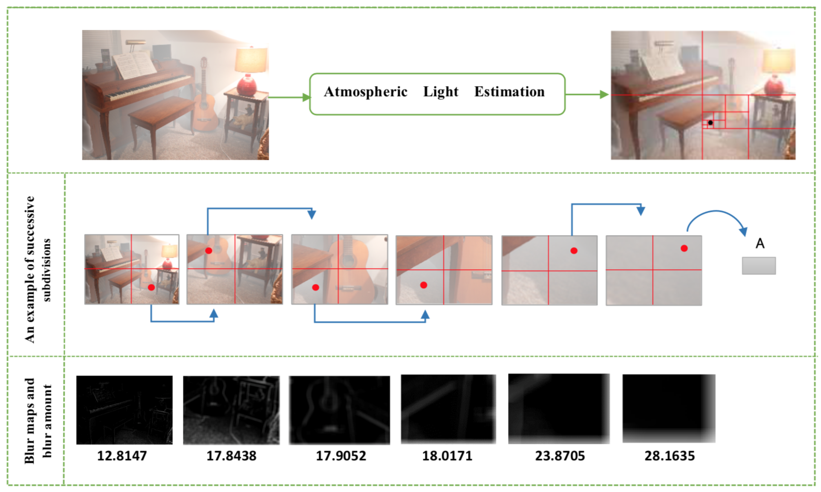
A practical example of proposed algorithm “A-Est”. The red spot indicates the region of interest (quadtree with maximum blur amount). The last row shows blur maps of each quadtree with the blur measure.
Figure 4.
A practical example of proposed algorithm “A-Est”. The red spot indicates the region of interest (quadtree with maximum blur amount). The last row shows blur maps of each quadtree with the blur measure.

Figure 5.
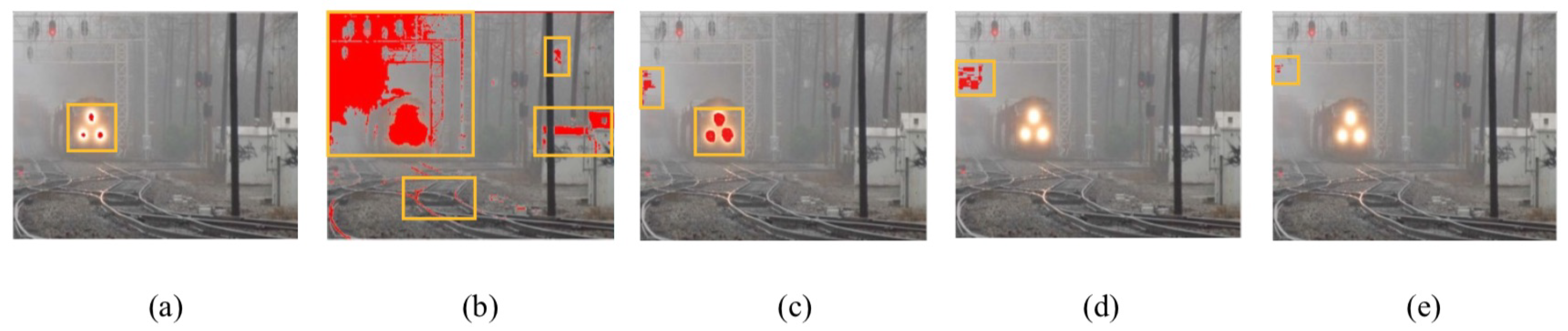
Parts of interest for estimating AL in different existing dehazing methods and the proposed one: (a) Zhu’s method [20]; (b) Sulami’s method [38]; (c) Salazar-Colores’s method [35]; (d) Haouassi’s method [36]; and (e) the proposed method.

Figure 6.
Visual comparison of AL estimation results for haze removal: (a) Zhu’s method [20]; (b) Cai’s method [26]; (c) Sulami’s method [38]; (d) Salazar-Colores’s method [35]; (e) Haouassi’s method [36]; and (f) the proposed method.

Figure 7.
General proposed architecture CMTnet.

Figure 8.
Internal Structure of Both D-unit and MCNN: (left) D-unit; and (right) MCNN.

Figure 9.
ReLU and BReLU Representations.

Figure 10.
Learning Process Illustration.

Figure 11.
The values of MSE and SSIM in terms of number of used D-units for some tested images: (left) MSE; and (right) for SSIM.
Figure 11.
The values of MSE and SSIM in terms of number of used D-units for some tested images: (left) MSE; and (right) for SSIM.

Figure 12.
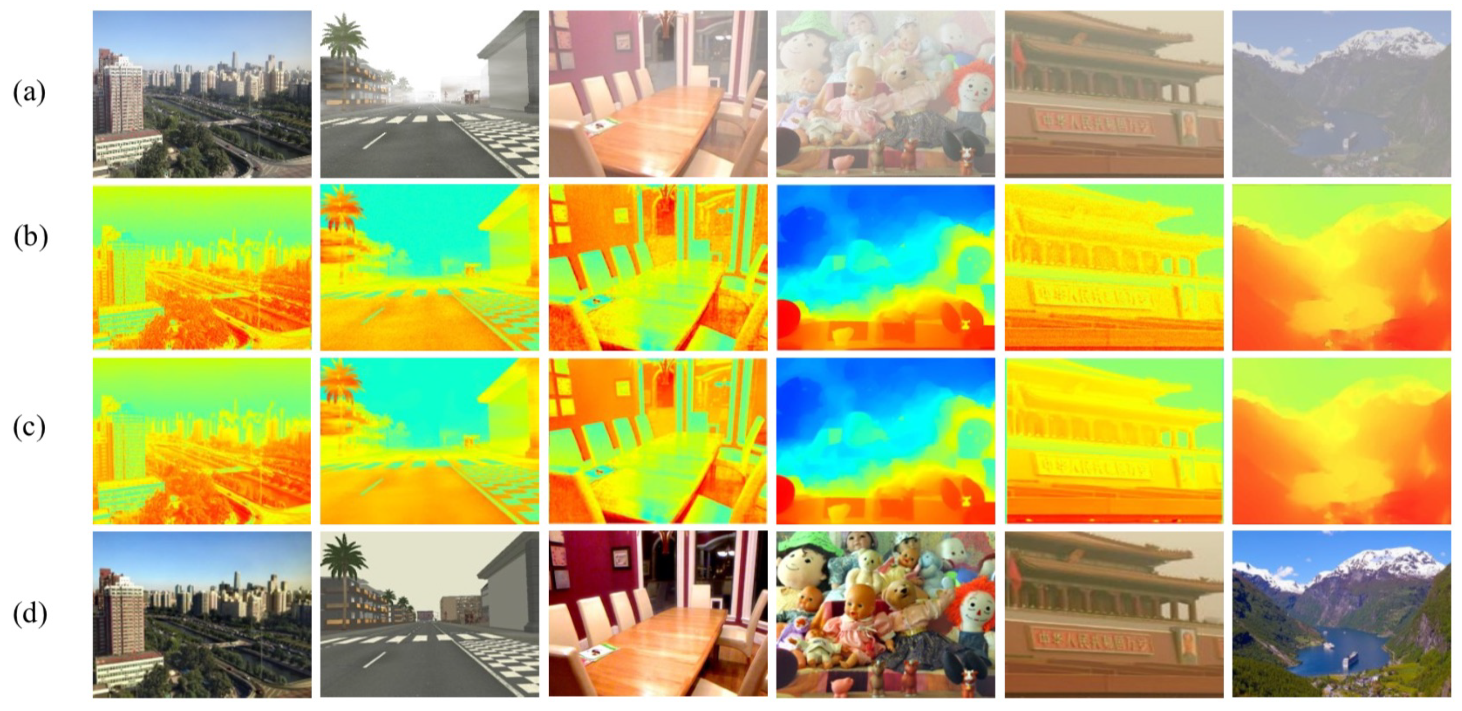
Visual results of proposed model: (a) hazy images; (b) rough transmission map ; (c) refined transmission map t; and (d) dehazed images.
Figure 12.
Visual results of proposed model: (a) hazy images; (b) rough transmission map ; (c) refined transmission map t; and (d) dehazed images.

Figure 13.
Samples of visual comparison of proposed system’s results with the comparative methods on synthetic indoor hazy images: (a) hazy image; (b) He’s method [14]; (c) Cai’s method [28]; (d) Ren’s method [26]; (e) Li’s method [40]; (f) Salazar’s method [35]; (g) our method; and (h) ground truth.

Figure 14.
Samples of visual comparison of proposed system’s results with the comparative methods on synthetic outdoor hazy images: (a) hazy image; (b) He’s method [14]; (c) Cai’s method [28]; (d) Ren’s method [26]; (e) Li’s method [40]; (f) Salazar’s method [35]; (g) our method; and (h) ground truth.

Figure 15.
Samples of visual comparison of proposed system’s results with the comparative methods on real-world hazy images: (a) hazy image; (b) He’s method [14]; (c) Cai’s method [28]; (d) Ren’s method [26]; (e) Li’s method [40]; (f) Salazar’s method [35]; and (g) our method.

Figure 16.
Visual comparison on nighttime hazy images: (a) hazy image; (b) He’s method [14]; (c) Cai’s method [28]; (d) Ren’s method [26]; and (e) our method;.


Table 1.
Summary of AL estimation methods used in existing and proposed dehazing approaches.
| Zhu 2015 [20] | Cai 2016 [28] | Sulami 2018 [38] | Salazar-Colores 2018 [35] | Haouassi 2019 [36] | Proposed |
|---|---|---|---|---|---|
| Top 0.1% brightest pixels in depth map | Fixed value (A = 1) | Twice PCA on all haze patches | Top 0.1% brightest pixels in | Top 0.1% brightest pixels in most blurry region with min energy | Top 0.1% blurred pixels |
Table 2.
Number of D-units and their corresponding average values of MSE and SSIM in each subNetwork.
Table 2.
Number of D-units and their corresponding average values of MSE and SSIM in each subNetwork.
| CMCNN | Nbre-U | 1-U | 2-U | 3-U | 4-U | 5-U | 6-U |
| MSE-Val | 1.96 | 1.42 | 1.06 | 0.62 | 0.61 | 0.61 | |
| CMCNN | Nbre-U | 1-U | 2-U | 3-U | 4-U | 5-U | 6-U |
| SSIM-Val | 0.87 | 0.94 | 0.94 | 0.94 | 0.95 | 0.95 |
Table 3.
The average values of MSE, SSIM, e, , FADE, and T on synthetic hazy images of the comparative methods.
Table 3.
The average values of MSE, SSIM, e, , FADE, and T on synthetic hazy images of the comparative methods.
| Method | He et al. [14] | Cai et al. [28] | Ren et al. [26] | Li et al. [40] | Salazar-Colores et al. [35] | Ours |
|---|---|---|---|---|---|---|
| SSIM | 0.727 | 0.853 | 0.821 | 0.898 | 0.887 | 0.912 |
| MSE | 2.093 | 2.892 | 0.846 | 1.867 | 0.079 | 0.068 |
| e | 1.896 | 1.452 | 1.237 | 2.190 | 2.830 | 2.792 |
| 2.951 | 2.763 | 2.609 | 3.652 | 4.025 | 3.785 | |
| FADE | 1.957 | 0.862 | 1.487 | 0.353 | 0.320 | 0.167 |
| T(s) | 14.901 | 1.004 | 1.830 | 0.469 | 0.541 | 0.386 |
Table 4.
The average values of e, , FADE, and T on real-world hazy images of the comparative methods.
Table 4.
The average values of e, , FADE, and T on real-world hazy images of the comparative methods.
| Method | He et al. [14] | Cai et al. [28] | Ren et al. [26] | Li et al. [40] | Salazar-Colores et al. [35] | Ours |
|---|---|---|---|---|---|---|
| e | 1.973 | 1.552 | 1.270 | 2.952 | 3.193 | 2.095 |
| 2.813 | 3.001 | 2.287 | 3.077 | 3.982 | 4.190 | |
| FADE | 2.172 | 0.903 | 1.816 | 0.534 | 0.510 | 0.289 |
| T(s) | 16.033 | 1.002 | 2.071 | 0.658 | 0.782 | 0.453 |
© 2020 by the authors. Licensee MDPI, Basel, Switzerland. This article is an open access article distributed under the terms and conditions of the Creative Commons Attribution (CC BY) license (http://creativecommons.org/licenses/by/4.0/).
Share and Cite
MDPI and ACS Style
Haouassi, S.; Wu, D. Image Dehazing Based on (CMTnet) Cascaded Multi-scale Convolutional Neural Networks and Efficient Light Estimation Algorithm. Appl. Sci. 2020, 10, 1190. https://0-doi-org.brum.beds.ac.uk/10.3390/app10031190
AMA Style
Haouassi S, Wu D. Image Dehazing Based on (CMTnet) Cascaded Multi-scale Convolutional Neural Networks and Efficient Light Estimation Algorithm. Applied Sciences. 2020; 10(3):1190. https://0-doi-org.brum.beds.ac.uk/10.3390/app10031190
Chicago/Turabian StyleHaouassi, Samia, and Di Wu. 2020. "Image Dehazing Based on (CMTnet) Cascaded Multi-scale Convolutional Neural Networks and Efficient Light Estimation Algorithm" Applied Sciences 10, no. 3: 1190. https://0-doi-org.brum.beds.ac.uk/10.3390/app10031190
Note that from the first issue of 2016, this journal uses article numbers instead of page numbers. See further details here.