Prediction of Soil-Available Potassium Content with Visible Near-Infrared Ray Spectroscopy of Different Pretreatment Transformations by the Boosting Algorithms

Featured Application

Quantitative models for visible near-infrared ray spectroscopy have rarely been exploited for the measurement of soil-available potassium. These results show that the predictors of soil-available potassium exhibit different influences with 29 pretreatment methods and eight regression algorithms. We found that a combination of three methods, Savitzky–Golay, standard normal variate, and dislodge tendency, had better stability than other pretreatment methods. The boosting algorithms that form an ensemble of multiple weak predictors have better accuracy and stability than other regression algorithms. Therefore, a more robust and trustworthy visible near-infrared ray (VIS-NIR) model is proposed, which can be used across industries to quantify the soil-available potassium concentration.

Abstract

The application of visible near-infrared (VIS-NIR) analysis technology to quantify the nutrients in soil has been widely recognized. It is important to improve the performance of regression models that can predict the soil-available potassium concentration. This study collected soil samples from southern Anhui, China, and concentrated on the modelling methods by using 29 pretreatment methods. The results show that a combination of three methods, Savitzky–Golay, standard normal variate, and dislodge tendency, exhibited better stability than others because it was the most capable of achieving levels A and B of the ratio of performance of deviation. The boosting algorithms that form an ensemble of multiple weak predictors exhibited better performance than partial least square (PLS) regression and support vector regression (SVR) for the prediction of soil-available potassium. These regression models could be employed to precisely predict the soil-available potassium concentration.

1. Introduction

Soil-available potassium is one of the most important nutrients for crop growth, and its availability is related to the soil organic matter content. Therefore, it is of great significance to guide fertilization and promote the development of precision agriculture by the rapid and accurate acquisition of soil-available potassium nutrient information. However, traditional methods used to detect soil nutrient information are all based on chemical analysis and have high requirements for detection personnel, low detection efficiency, high cost, a likelihood of causing environmental pollution, and other problems, and can no longer meet the development requirements of modern precision agriculture. In recent years, near-infrared analysis technology has received increasing attention for the quantitative determination of soil nutrients due to its advantages of easy operation and no pollution [1,2,3,4,5,6].

Visible near-infrared ray (VIS-NIR) spectroscopy of soil nutrient elements mainly focuses on organic matter, nitrogen, and water, and only a few studies have focused on the quantitative prediction of soil-available potassium. Some experts have researched the application of VIS-NIR spectroscopy for the determination of soil-available potassium. He et al. utilized infrared spectroscopy and the Least-squares support vector machines(LS-SVM ) model to predict the nitrogen, phosphorus, and potassium concentrations in soil in 2011 [7]. Liu Xuemei and Liu Jian-She utilized the standard normal variate (SNV), multiplicative scatter correction (MSC), and Savitzky–Golay (SG) methods for pretreatment in the VIS-NIR spectral range, which is only from 325 to 1075 nm. The results showed that the coefficient of determination (R²) was 0.82 and 0.72 for available phosphorus and available potassium in soil, respectively [8]. Jia Shengrao et al. used the recursive partial least squares(RPLS) method to detect the soil-available phosphorus and available potassium, and the R² and the ratio of performance of deviation (RPD) were 0.61 and 0.76 and 1.6 and 2.05, respectively [9]. The soil-available potassium content exhibits an unbalanced distribution; therefore, as the diversity of the soil samples increases, the difficulty in predicting soil properties accurately increases. Wang Wen-Jun et al. separated the available potassium content in soil into high and low levels, which were individually calibrated by the partial least squares (PLS) method, and showed that the difference in the soil-available potassium content might influence the performance of the VIS-NIR regression [10]. In these studies, these quantitative prediction methods were meaningful for the analysis of these spectral algorithms [7,8,9,10,11]. Despite VIS-NIR spectroscopy having been extensively used for the prediction of soil nutrients, the regression model for soil-available potassium exhibited the worst performance. Consequently, the main purpose of this study is to gain an understanding of the pretreatment and regression algorithm required for VIS-NIR spectroscopy to determine the impact of soil-available potassium; thus, this study not only compares various pretreatment and regression methods but also finds the advantage of those methods.

This research mainly studied yellow loam in southern Anhui Province. Through field soil sampling, indoor physical and chemical analysis, spectral acquisition, pretreatment methods, and so on, a series of working, valid boosting regression algorithms were calibrated for soil-available potassium content with a near-infrared spectrum. Meanwhile, the performance of these models was evaluated via the RPD and ratio of performance to interquartile distance (RPIQ) to analyze the reliability and stability of soil-available potassium predictions. This manuscript also provides a reference for the remote sensing monitoring of soil information.

2. Materials and Methods

2.1. Experimental Materials

Yellow loam is a classic soil in Anhui, China. Thus, the sample collection areas were Yellow Mountain and Shi Tai. This experiment collected 188 samples by diagonal sampling, from which rocks and debris were removed. Then, all of the soil samples were brought back to the laboratory and naturally air-dried in a ventilated environment. After drying, the soil was ground and screened to 2 mm, and each soil sample was divided into two parts, one for use in a hyperspectral experiment as shown in Figure 1 and the other for chemical testing of the flame photometer [12].

The chemical testing of the flame photometer was completed by other professional testing organizations to determine the concentration of soil-available potassium. The VIS-NIR measurements of the soil were conducted in the laboratory utilizing Ocean Optics OFS1700, the parameters of which indicate that the spectral range is 350–1700 nm, and the spectral resolution is 2 nm within the spectral range of 350–900 nm, and 5 nm within the spectral range of 900–1700 nm. Soil powder was placed into the sample containers with the insides covered with black cloth. Then, three sets of each sample were randomly selected for spectral measurement, and the average spectra were taken as the original spectrum of the soil.

2.2. Pretreatment Transformations

The basic pretreatment transformations for VIS-NIR are Savitzky–Golay (SG), first derivative (FD), second derivative (SD), standard normal variate (SNV), multiplicative scatter correction (MSC), logarithmic transformation (LG), mean centre (MC), and dislodge tendency (DT) [13,14,15,16]. The SG method is very important to guarantee that the edge band is removed from the spectral curve, which has extensive noise, and this process improves the signal-to-noise ratio, enhances the function of the central wavelength point, and retains the peak characteristics of the original spectral signal to the greatest extent. FD and SD can both eliminate the effect of the linear baseline but result in amplified noise. SNV calibrates the effects of soil particle size and surface scattering [17]. MC and DT both reduce the spectral offset. Therefore, this manuscript combined the 29 pretreatment algorithms that are shown in

Table 1. Pretreatment methods applied to the visible near-infrared (VIS-NIR) of soil samples.

Pretreatment Method	Abbreviations
Reflection spectrum without pretreatment method	RS
First derivative	FD
Second derivative	SD
Standard normal variate	SNV
Multiplicative scatter correction	MSC
Logarithmic transformation	LG
Mean center	MC
Dislodge tendency	DT
Dislodge tendency with standard normal variate	SNV + DT
First derivative with standard normal variate	SNV + FD
Second derivative with standard normal variate	SNV + SD
First derivative with multiplicative scatter correction	MSC + FD
Second derivative with multiplicative scatter correction	MSC + SD
First derivative with logarithmic transformation	LG + FD
Second derivative with logarithmic transformation	LG + SD
Savitzky–Golay	SG
First derivative with Savitzky–Golay	SG + FD
Second derivative with Savitzky–Golay	SG + SD
Standard normal variate with Savitzky–Golay	SG + SNV
Multiplicative scatter correction with Savitzky–Golay	SG + MSC
Logarithmic transformation with Savitzky–Golay	SG + LG
Mean center with Savitzky–Golay	SG + MC
Dislodge tendency with Savitzky–Golay	SG + DT
Dislodge tendency with standard normal variate and Savitzky–Golay	SG + SNV + DT
First derivative with standard normal variate and Savitzky–Golay	SG + SNV + FD
Second derivative with standard normal variate and Savitzky–Golay	SG + SNV + SD
First derivative with multiplicative scatter correction and Savitzky–Golay	SG + MSC + FD
Second derivative with multiplicative scatter correction and Savitzky–Golay	SG + MSC + SD
First derivative with logarithmic transformation and Savitzky–Golay	SG + LG + FD
Second derivative with logarithmic transformation and Savitzky–Golay	SG + LG + SD

.

2.3. Regression Algorithms

In chemometrics, partial least square (PLS) regression and support vector regression (SVR) are commonly used to build calibration models [17,18,19]. PLS analysis was utilized as a method to extract the latent variables (LVs) of the spectrum. LVs are important to reduce the dimensionality and represent the main soil nutrition information for regression prediction. SVR, a state-of-the-art learning algorithm, has a theoretical foundation in machine learning methods [17]. PLS and SVR both utilize a kernel function to map input variables to a high-dimensional feature space, such as a sigmoid function and radial basis function (RBF). Therefore, the comparison of the performance of linear and nonlinear functions is essential for analyzing models of the soil-available potassium.

Gradient boosted regression trees (GBRTs) and adaptive boosting (AdaBoost) regression are ensemble boosting methods that can be used to reduce the error of any ‘weak’ learning machine by repeatedly running a given weak learning machine. GBRTs are a generalization of boosting to arbitrary differentiable loss functions and considers additive models of this following form:

$$\mathrm{F}\left(\mathrm{x}\right)={\displaystyle \sum }_{m=1}^M{\gamma }_m{h}_m\left(x\right)$$

(1)

where h_m is the newly added tree to minimize the loss L, and γ_m is the step length. GBRT requires a decision tree of fixed size for weak learning [20,21].

The AdaBoost regressor is a meta-estimator that begins by fitting a regression to the original dataset and then fitting additional copies of the regression to the same dataset, but the weight of the instances is adjusted according to the error of the current prediction [22]. The working mechanism of the AdaBoost method is illustrated in Figure 2. D(X) in the figure is the dataset with training samples. The AdaBoost method demonstrates little effect of the overfitting issue and shows better stability with noisy data.

In this work, GBRT and AdaBoost both utilized the decision tree for weak learning and the least squares as the loss function. The main parameter is equal to the number of weak learners that are named estimators. Therefore, estimators are important to obtain better performance of the GBRT and AdaBoost models.

2.4. Evaluation Metrics

This manuscript compares the accuracy and stability of different regression models of the VIS-NIR spectrum. Therefore, the evaluation metrics of the coefficient of determination (R²), root mean square error (RMSE), mean absolute error (MAE), and the ratio of performance of deviation (RPD) have been adopted to evaluate the prediction [7,8,9,10,11]. These methods have been widely used for regression models of the spectrum.

The RPD has been used for several years by NIR scientists working on agricultural products and has been widely appropriated by soil science researchers.

$$\mathrm{RMSE}=\sqrt{\frac{1}{n}{{\displaystyle \sum }}_{i=1}^n{\left(y_i-{\widehat{y}}_i\right)}^2}$$

(2)

$$\mathrm{RPD}=\frac{SD}{RMSE} = \sqrt{\frac{n{{\displaystyle \sum }}_{i=1}^n{\left(y_i-\overline{y}\right)}^2}{\left(n-1\right){{\displaystyle \sum }}_{i=1}^n{\left(y_i-{\widehat{y}}_i\right)}^2}}$$

(3)

SD is standard deviation.

Table 2. The ratio of performance of deviation (RPD) level.

RPD	Level
RPD ≥ 3.0	A
2.0 ≤ RPD < 3.0	B
1.5 < RPD < 2.0	C
RPD ≤ 1.5	D

shows the different levels of the model for the different RPD values.

The RPD value could be an important criterion, but Bellon-Maurel pointed out that soil physical properties and chemical contents both exhibit a biased normal distribution; therefore, the ratio of performance to IQ (RPIQ) value is more objective than RPD [23]. RPIQ is based on quartiles, which better represent the spread of the population. The quartiles are milestones in the population range: Q1 is the value below which we can find 25% of the samples; Q3 is the value below which we find 75% of the samples; and Q2, commonly called the median, is the value under which 50% of samples are found. RPIQ is the ratio of IQ to RMSE, where IQ is the difference between the third quartile Q3 and the first quartile Q1. A larger RPIQ value indicates improved model performance. The formula is shown as follows:

$$IQ=Q3-Q1$$

(4)

$$\mathrm{RPIQ}=\frac{IQ}{RMSE}=\frac{Q3-Q1}{\sqrt{\frac{1}{n}{{\displaystyle \sum }}_{i=1}^n{\left(y_i-{\widehat{y}}_i\right)}^2}}$$

(5)

The sum of ranking difference (SRD) is simple to understand the comparison of regression models and provides an easy tool to evaluate the methods [24,25]. Therefore, this manuscript compared the R², RMSE, MAE, RPD, RPIQ, and SRD of these regression models.

3. Results and Discussion

3.1. Dataset Statistics

The total number of soil samples was 188, which were split into a training set and a testing set by the Kennard–Stone (KS) method at the proportion of 7:3 [26], which is often used with VIS-NIR spectroscopy for model construction and model testing. The number of training sets was 131, and the number of testing datasets was 57. The data statistics are presented in

Table 3. Soil-available potassium sample statistics.

Type	Number	Max/mg·kg−1	Min/mg·kg−1	Average/mg·kg−1	Standard Deviation
Total	188	670	60	190.6	133.1
Train	131	670	60	190.7	134.7
Test	57	600	60	188.2	128.0

. Table 3 also reveals that the data distribution of the available potassium content of the soil in the training set is similar to that in the testing set.

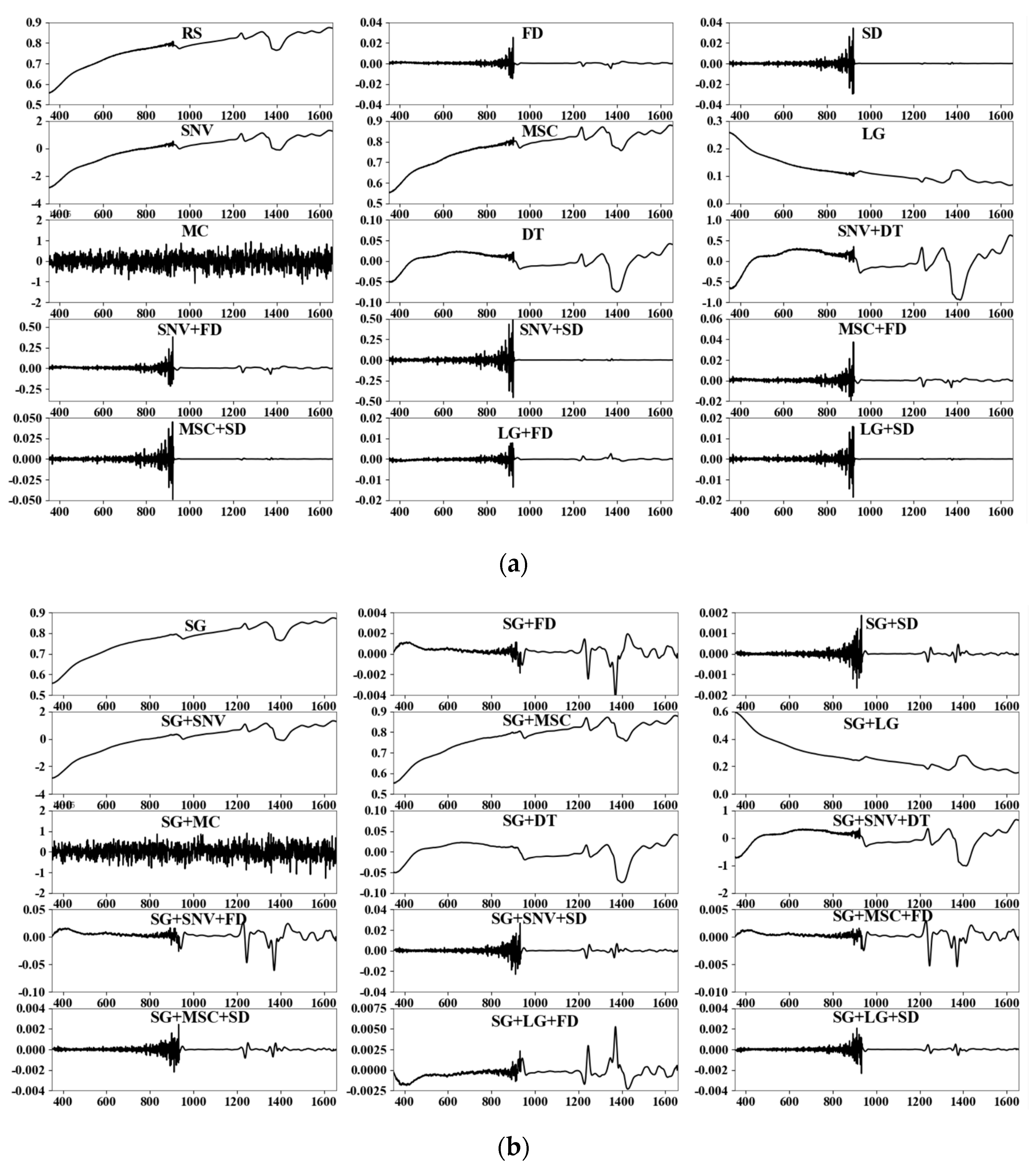
The pretreatment method is indispensable during the training of a regression model and is also a key step for quantifying the analysis of the VIS-NIR spectrum. Information on the VIS-NIR spectrum of soil would be effective to filter noise and reduce the complexity of the pretreatment methods, but different methods have different effects on various regression models. Figure 3 shows the VIS-NIR spectrum with 29 pretreatment methods and a reflection spectrum (RS). Figure 3a is without the SG method, and Figure 3b is the SG method. The SG method reduces the noise of the spectrum and makes the curve smoother. The DT method creates pristine peaks in the spectrum, but the peak value of the original spectrum becomes zero. MC not only reduces the spectral offset but also weakens the characteristic points of the spectrum. The two scattering correction methods of SNV and MSC did not significantly change the spectral curve. FD, SD, and LG made great changes to the VIS-NIR.

3.2. Performance of Regression Models with Different Pretreatment Methods

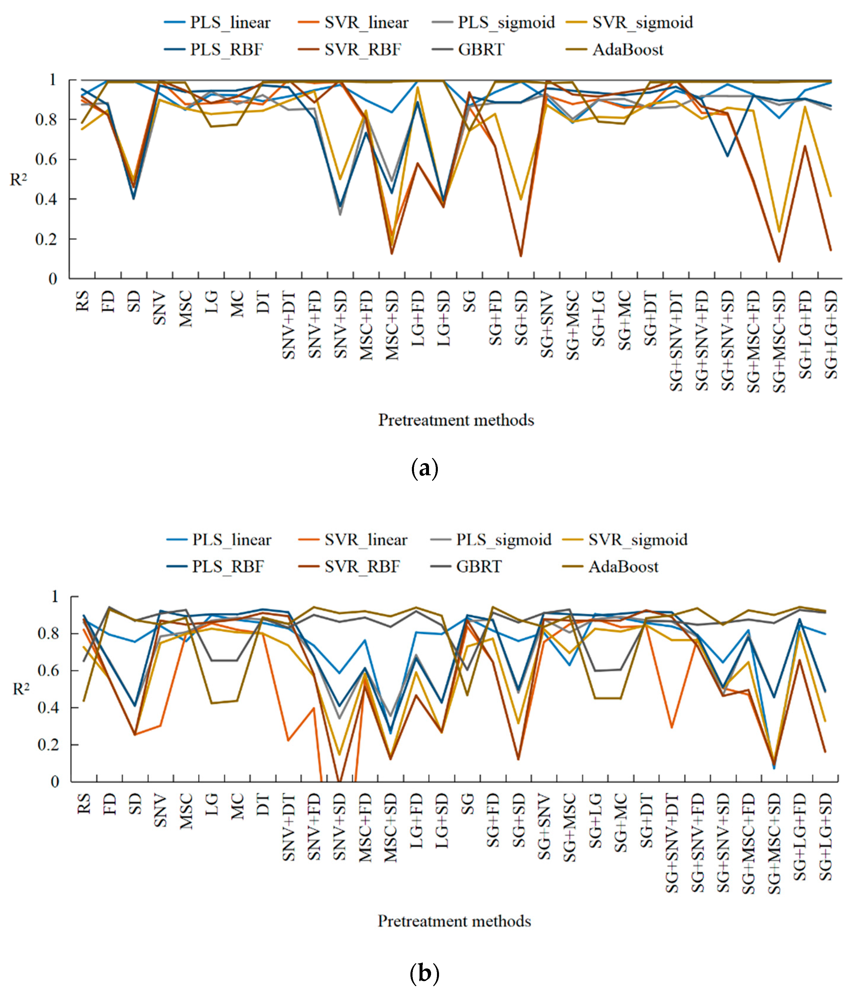
This study compares 240 regression models with eight regression algorithms and 29 pretreatment transformations for the VIS-NIR spectrum. Figure 4 exhibits the R² values for the training and testing sets of the regression models, and Figure 4a,b represent the prediction R² values for the training and testing datasets, respectively. With different pretreatment methods,

Table 4. RPD level of regression models with different pretreatment methods.

Pretreatment Methods	PLS_Linear	PLS_Sigmoid	PLS_RBF	SVR_Linear	SVR_Sigmoid	SVR_RBF	GBRT	AdaBoost
RS	B	B	B	C	D	B	D	D
FD	C	D	D	D	D	D	A	A
SD	C	D	D	D	D	D	B	B
SNV	B	B	A	D	C	B	A	B
MSC	C	B	A	C	C	B	A	B
LG	B	B	A	B	C	B	D	D
MC	B	B	A	C	C	B	D	D
DT	B	B	A	C	C	A	B	B
SNV + DT	B	B	A	D	C	A	B	B
SNV + FD	C	C	D	D	D	D	A	A
SNV + SD	C	D	D	D	D	D	B	A
MSC + FD	C	D	D	D	D	D	B	A
MSC + SD	D	D	D	D	D	D	B	B
LG + FD	C	D	D	D	D	D	A	A
LG + SD	B	D	D	D	D	D	B	B
SG	B	B	B	C	D	B	D	D
SG + FD	C	B	B	D	C	D	A	A
SG + SD	C	D	D	D	D	D	B	B
SG + SNV	B	B	A	C	B	B	A	B
SG + MSC	D	B	A	B	D	B	A	B
SG + LG	B	B	A	B	C	B	D	D
SG + MC	B	B	A	C	C	B	D	D
SG + DT	B	B	A	C	B	A	B	B
SG + SNV + DT	B	B	A	D	C	A	A	A
SG + SNV + FD	B	B	B	C	C	C	B	A
SG + SNV + SD	C	D	D	D	D	D	B	B
SG + MSC + FD	B	B	B	D	D	D	B	A
SG + MSC + SD	D	D	D	D	D	D	B	B
SG + LG + FD	B	B	B	D	C	D	A	A
SG + LG + SD	B	D	D	D	D	D	A	A

and Figure 5 exhibit the RPD levels and RPIQ of the regression models.

The nonlinear function was employed to train PLS and SVR. Therefore, the PLS models with linear, sigmoid, and RBF functions are respectively referred to as PLS_linear, PLS_sigmoid, and PLS_RBF, and the SVR models with linear, sigmoid, and RBF functions are respectively named SVR_linear, SVR_sigmoid, and SVR_RBF. RS indicates the VIS-NIR without any pretreatment. Thus, the results show that a few of the pretreatment datasets exhibit worse model performance than the RS dataset. In particular, the SVR algorithm has more models with R² values lower than 0.2 compared with the PLS algorithm in Figure 4. Following the consideration of the pretreatment methods, the R² value of PLS_linear with SG + MSC + SD was determined to be less than 0.2. However, R² values of SVR linear with MSC + SD, SG + SD, SG + LG + FD and SG + LG + SD are less than 0.2, but the R² value of PLS with a nonlinear function (sigmoid and RBF) is not only greater than 0.2 but also better than that of SVR. Therefore, PLS with a nonlinear function is more suitable for the regression prediction of VIS-NIR. In Figure 4, the R² values of the boosting algorithms are all greater than 0.4, which means that the boosting regression algorithm is preferable to the other methods. In particular, the R² of GBRT with the testing dataset is considerably greater than 0.5, and the R² with the training dataset is close to 1. Therefore, it is significant to choose adaptive pretreatment and regression algorithms to predict the content of soil-available potassium by VIS-NIR.

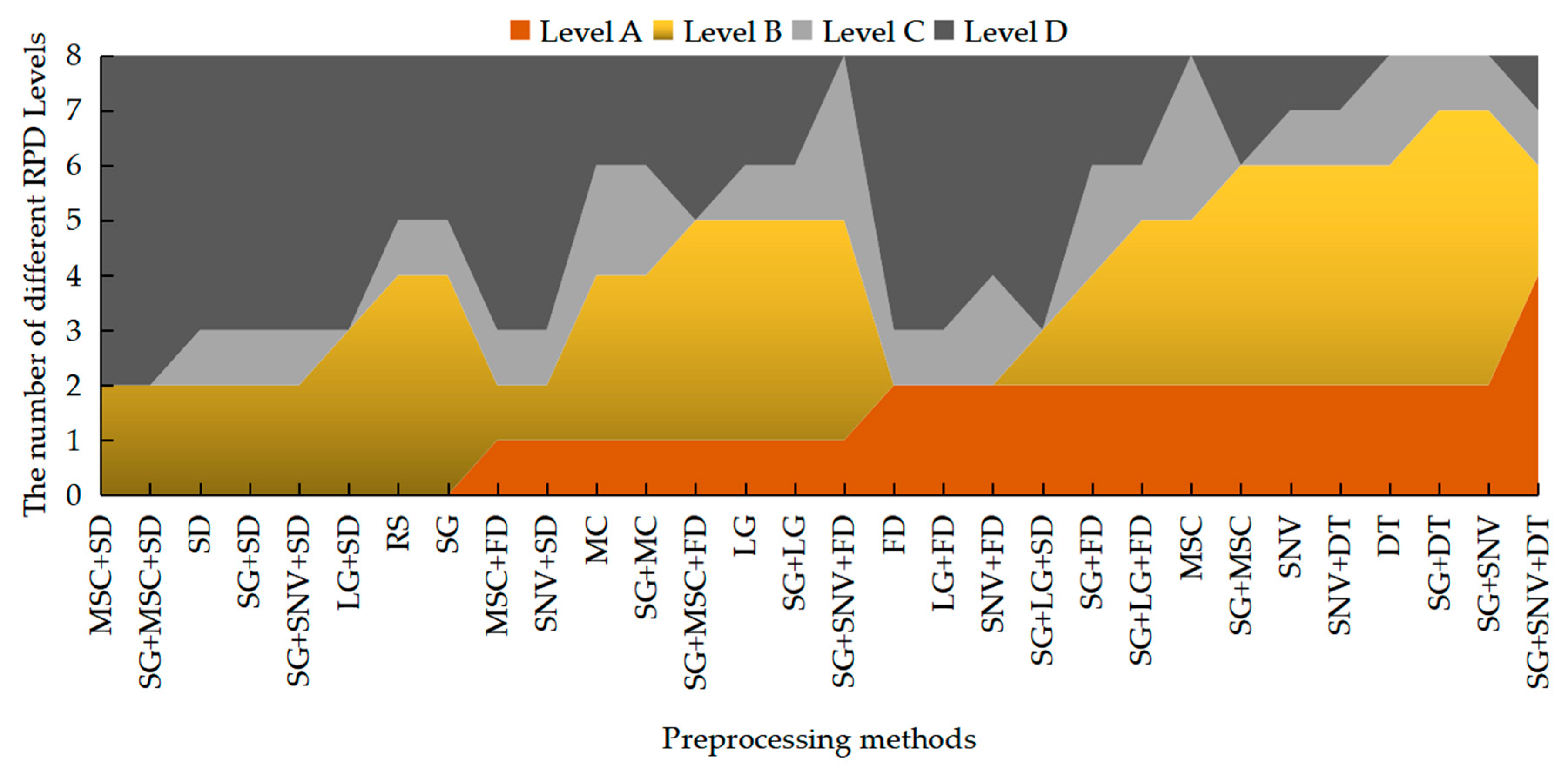
In Table 4, the RPD level of the regression models is compared to determine the influence of the different pretreatment methods based on the testing dataset. Level A denotes that the regression model has the best stability, and level D means the worst. The RPD using the RS dataset as a baseline shows that a level A model is difficult to achieve without pretreatment. SVR_sigmoid, GBRT, and AdaBoost on the RS dataset are level D, but the PLS algorithm with linear and nonlinear functions was level B. The regression of the RBF kernel function using partial pretreatment methods could achieve level A, but the model with linear and sigmoid kernel functions could not attain level A, even if all pretreatment methods were used. In conclusion, regression algorithms and pretreatment methods are significant for the prediction of the VIS-NIR of soil-available potassium, as shown in Table 4. Table 4 reveals that the prediction performance of different pretreatment methods at different levels.

Through the statistics, Figure 5 shows the visualization of the RPD level of models with 29 pretreatment methods and RS in order. The black areas represent level D, the grey areas represent level C, the yellow areas represent level B, and the orange areas represent level A. There are six pretreatment methods, and RS could not achieve level A with any regression algorithms. Only the SG + SNV + DT method has four models with RPD level A, and SG + DT and SG + SNV not only have two models with RPD level A and five models with RPD level B but also have only one model with RPD level C and zero models with RPD level D. Therefore, SG + DT, SG + SNV, and SG + SNV + DT are the most stable pretreatment methods for the prediction of soil-available potassium with regression algorithms.

Table 5. The number of different models at varying RDP levels.

RPD	PLS_Linear	PLS_Sigmoid	PLS_RBF	SVR_Linear	SVR_Sigmoid	SVR_RBF	GBRT	AdaBoost
Level A	0	0	12	0	0	4	11	11
Level B	17	18	6	3	2	10	13	13
Level C	10	1	0	9	12	1	0	0
Level D	3	11	12	18	16	15	6	6

shows the number of models with different RPD levels. The statistics show that the number of PLS_RBFs with level A is the highest, but the boosting algorithms represent more stability because GBRT and AdaBoost show the highest numbers of models with level A and level B, showing that these levels were both meaningful for predicting the content of soil-available potassium. Therefore, the boosting algorithms are better than PLS and SVR with linear and nonlinear functions.

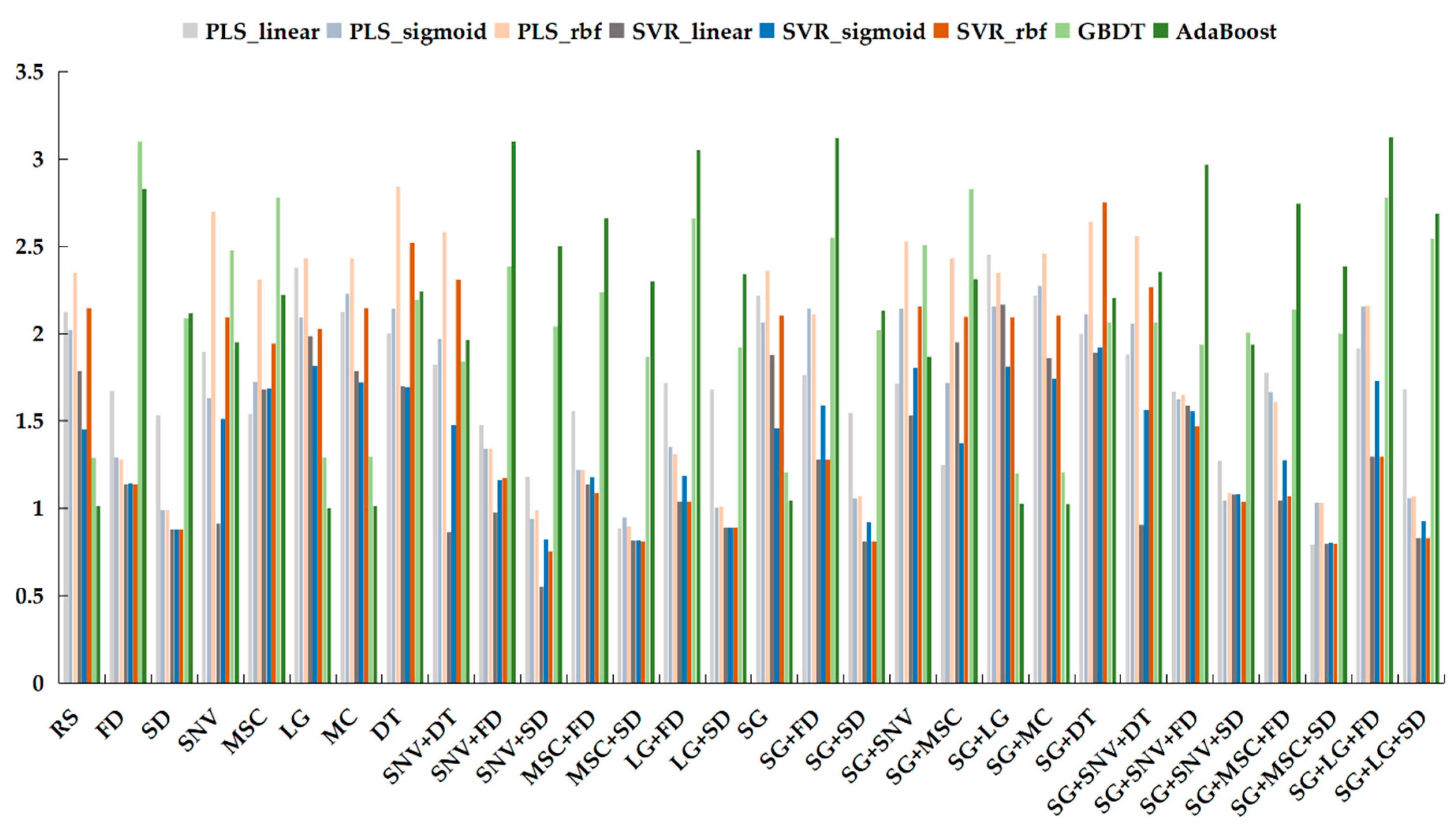
Figure 5 and Table 5 indicate that there are few models at level A; therefore, other evaluation metrics are needed. The RPIQ value was computed as an important evaluation metric and is presented in Figure 6 because the content of soil-available potassium has a biased normal distribution. The green color represents the RPIQ values of GBRT and AdaBoost on the testing dataset. Figure 6 shows that most of the pretreatment datasets exhibited improved performance when boosting regression algorithms were used for prediction of the content of soil-available potassium. Dark green indicates the RPIQ values for AdaBoost with all pretreatment methods. AdaBoost performed extremely well with SNV + FD, LG + FD, SG + FD, SG + SNV + FD, and SG + LG + FD because the RPIQ values were greater than 3. Additional methods all had values less than 3, except for GBRT with DF. The RPIQ value of SG + LG + FD is the maximum for AdaBoost. As a result, the next part is the comparison and analysis of the best regression models.

3.3. The Best Regression Models of Visible Near-Infrared (VIS-NIR)

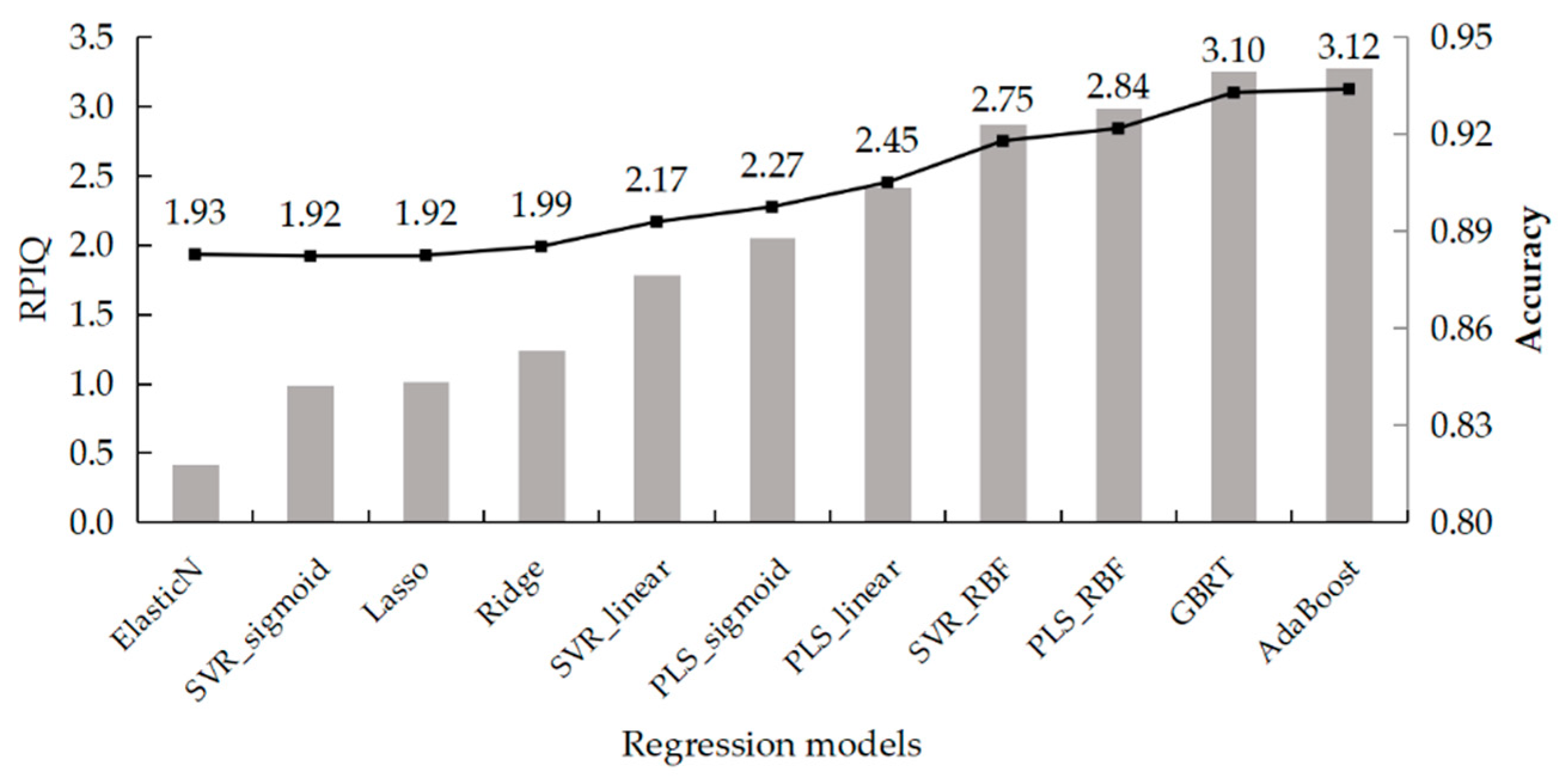
This manuscript demonstrates the performance of all the best models that not only contain PLS, SVR, and boosting but also ElasticNet, Lasso, and Ridge [27,28] because these three methods are also used frequently.

Table 6. The performance and parameters of the best regression models.

Regression Model	Training Dataset		Testing Dataset		RPD Level	Pretreatment Methods	Parameters
	R2	RMSE	R2	RMSE
PLS_linear	0.90	44.3	0.903	39.8	B	SG + LG	LVs = 14
PLS_sigmoid	0.90	42.4	0.887	42.9	B	SG + MC	LVs = 16, Gamma = 0.005
PLS_RBF	0.97	23.3	0.928	34.3	A	DT	LVs = 27, Gamma = 0.1
SVR_linear	0.90	42.5	0.876	45.0	B	SG + LG	C = 40,000
SVR_sigmoid	0.88	47.1	0.842	49.8	B	SG + DT	C = 1,270,000, Gamma = 0.005
SVR_RBF	0.95	28.9	0.923	35.5	A	SG + DT	C = 150,000, Gamma = 0.1
GBRT	0.99	5.53	0.939	31.5	A	FD	Estimators = 3100
AdaBoost	0.99	13.7	0.941	31.2	A	SG + LG + FD	Estimators = 100
ElasticNet	0.84	53.2	0.818	54.6	C	SG + FD	L1 = 0.3, Alpha = 2 × 10−6
Lasso	0.83	56.3	0.843	50.7	B	SG	Alpha = 0.02
Ridge	0.9	41.9	0.853	49.0	B	SG + LG + FD	Alpha = 0.0001

shows that PLS, SVR, and boosting algorithms are the best because the RPD levels of ElasticNet, Lasso, and Ridge are only level B or level C. The best model for the PLS algorithm is PLS_RBF, which has LV and Gamma parameters of 27 and 0.1, respectively. The LVs of PLS_linear and PLS_sigmoid are 14 and 16, respectively. The best model for the SVR algorithm is SVR_RBF, which has C and Gamma parameters of 150,000 and 0.1, respectively. The kernel function of RBF is shown to be better than the linear and sigmoid functions. The C values of SVR_linear and SVR_sigmoid are 40,000 and 1,270,000, respectively. The number of estimators is 3100 and 100, respectively, for GBRT and AdaBoost. Considering the R² of these best models, PLS_linear, PLS_RBF, SVR_RBF, GBRT, and AdaBoost are over 0.9 with the testing dataset, and the RPD level of only PLS_linear is B. The best pretreatment methods for PLS_RBF, SVR_RBF, GBRT, and AdaBoost are DT, SG + DT, FD, SG + LG + FD, respectively. Therefore, different regression algorithms correspond to different pretreatment datasets to achieve optimal performance.

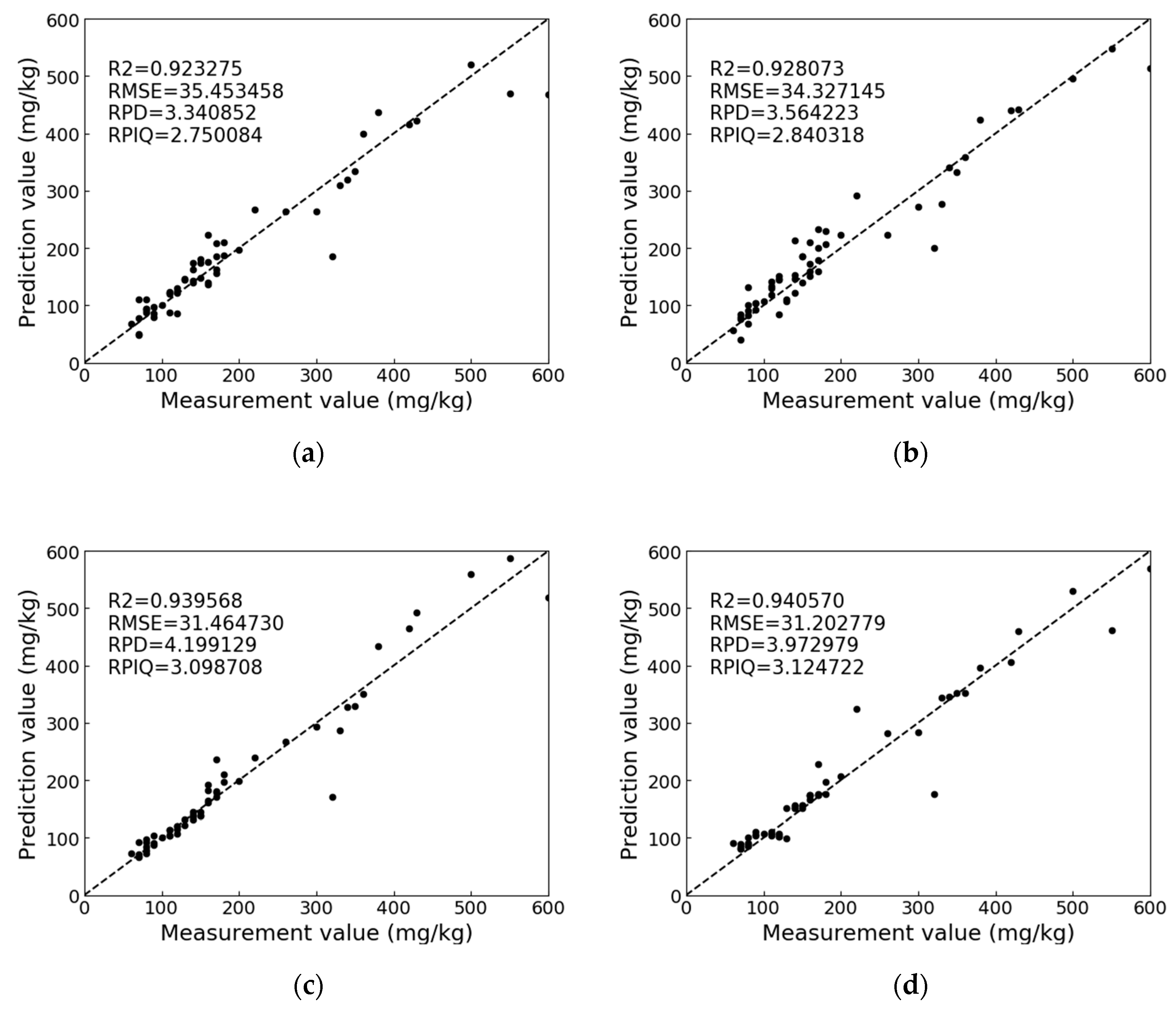
Figure 7 shows the RPIQ values of the best models from the discrete levels of the RPD value. The values of SVR_RBF, PLS_RBF, GBRT, and AdaBoost are more important than those of the other methods, and GBRT and AdaBoost are preferable to PLS_RBF and SVR_RBF.

Figure 8 shows the comparison diagram of SVR_RBF, PLS_RBF, GBRT, and AdaBoost with the testing dataset. The details of the evaluation metrics show that the RPD value of GBRT is higher than that of AdaBoost, but AdaBoost has better accuracy and stability than GBRT from the comparison of RPIQ values. Meanwhile, the R² and RMSE values of AdaBoost are also preferable to those of GBRT. Through the above analysis, the AdaBoost algorithm was determined to exhibit the best performance in predicting the soil-available potassium content by VIS-NIR.

3.4. Two Sub-Ranges of Soil-Available Potassium by Boosting Methods

From the data in Table 3, the soil-available potassium concentration range was between 60–670 ppm for the training set and 60–600 ppm for the test set, with the average lying at approximately 190 ppm. In addition, given that the concentration range is so wide and the average is below 200 ppm, the concentration range was split into two sub-ranges. A ‘low concentration’ between 60 and 300 ppm and a ‘high concentration’ between 300 and 600 ppm were trained by two boosting algorithms for a more robust and trustworthy model.

The samples were separated into two sub-ranges, and the number of low- and high-concentration samples was 148 and 40, respectively.

Table 7. Low concentration of soil-available potassium sample statistics.

Type	Number	Max/mg·kg−1	Min/mg·kg−1	Average/mg·kg−1	Standard Deviation
Total	148	290	60	129.73	46.35
Train	104	290	60	130.19	47.23
Test	44	260	60	128.63	44.19

and

Table 8. High concentration of soil-available potassium sample statistics.

Type	Number	Max/mg·kg−1	Min/mg·kg−1	Average/mg·kg−1	Standard Deviation
Total	40	670	300	416	101.7
Train	28	670	300	415	101.3
Test	12	630	300	418.3	102.5

show the statistics.

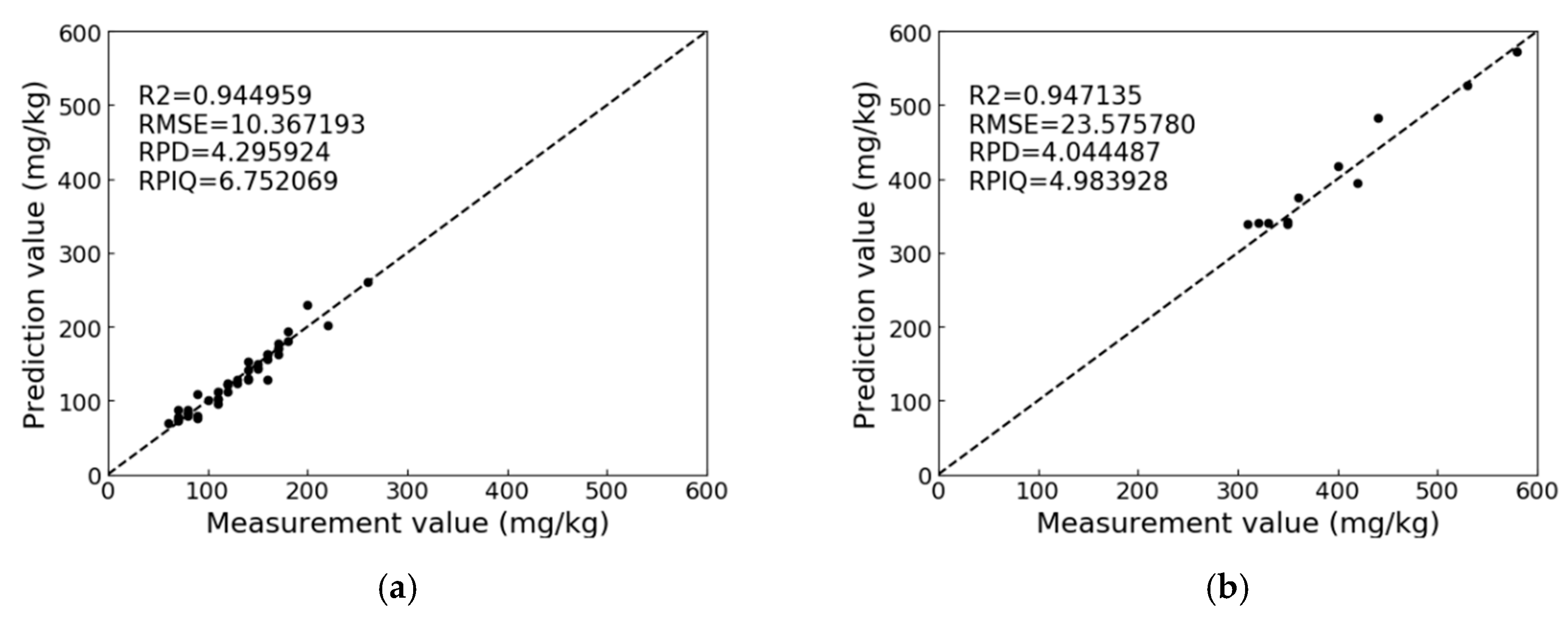
GBRT and AdaBoost are trained and tested with all pretreatment methods. Figure 9 shows the best prediction with the low concentration and high concentration. For the low concentration, the AdaBoost with 2000 estimators is the best. The pretreatment method for this model is SG + SNV + DT. The best R², RPD and RPIQ values of the low concentrations are 0.945, 4.3 and 6.75, respectively. For the high concentration, the GBRT with 400 estimators is the best, and the pretreatment method is SG + SNV + FD. The best R², RPD, and RPIQ values of high concentrations are 0.947, 4.04, and 4.98, respectively. Figure 9 shows that the AdaBoost and GBRT methods have accurate and stabilized predictions of soil-available potassium.

3.5. Discussion

Based on VIS-NIR spectroscopy, training and testing datasets were established with the original spectral reflectance and 29 pretreatments. These pretreatment methods include Savitzky–Golay (SG), first derivative (FD), second derivative (SD), standard normal variate (SNV), multiplicative scatter correction (MSC), logarithmic transformation (LG), mean center (MC), dislodge tendency (DT), and various combinations of these methods. However, not all pretreatment methods are effective, and SG, SNV, FD, and MSC are used more frequently than the other methods [8,19,29,30]. As a standard preparation of the soil spectral curves, Savitzky–Golay appears in almost every application [30]. In this manuscript, the performance shows that MSC + SD, SG + MSC + SD, SD, SG + SD, SG + SNV + SD, and LG + SD are worse than RS. In paticular for SD, only SNV + SD and SG + LG + SD achieved RPD level A, and the best models were entirely without the SD method. The SD method may be seriously disturbed by the features of the VIS-NIR. Therefore, the SD pretreatment method was not useful for the prediction of the VIS-NIR spectrum of the soil-available potassium content. Twenty-three pretreatment methods were better than RS, 10 without SG and 13 with SG. Only three of the methods did not include SG from the best 11 models. Therefore, the SG method has a great influence on the prediction of soil-available potassium content. The frequency of the DT method is most common after SG in the best models, and the DT is a transformation that usually occurs after SNV. Hence, SG + SNV + DT is the best pretreatment method in this study, with most models at RPD level A.

The different regression models have linear and nonlinear kernel functions. From Table 6 of this manuscript, the linear regression models are more stabilized, especially PLS_linear, which has the fewest number of models with RPD level D. The sigmoid kernel function is the worst, and the RBF kernel function is better than linear functions. The best models of PLS and SVR are PLS_RBF and SVR_RBF. The accuracy of the regression model with the RBF function reached the best performance. Therefore, the feature of the VIS-NIR follows the normal distribution. The methods of PLS [9,10,29,30] and SVR [17,18] are widely used for the calibration of VIS-NIR spectra, but boosting regression algorithms are almost never used. GBRT and AdaBoost, which are boosting algorithms, can be effectively calibrated to predict the soil-available potassium content. Boosting is a frame algorithm that produces a predictor in the form of an ensemble of multiple weak predictors. GBRT improves the prediction accuracy by building each decision tree for the past residuals rather than the response variable [21]. The AdaBoost algorithm trains a weak classifier step by step, and every weak classifier is trained on a different weight set of the sample subset. Then, a strong classifier is finally constructed by selecting each training iteration [22]. GBRT calculates the gradient value to locate the deficiency of the model, but AdaBoost is based on loss assessment of the prediction to adjust the weight of the sample subset. From the above figure and table, both algorithms have better performance than other regression algorithms. GBRT and AdaBoost both exhibit the best prediction of soil-available potassium content by VIS-NIR. It is important to solve the problem of fairly comparing the models [24,25]. For VIS-NIR model analysis, the common evaluation metrics are the coefficient of determination, root mean square error, mean absolute error, residual predictive deviation, and the ratio of performance to IQ [7,8,9,10,29,30]. The accuracy of the models can be weighed by R², RMSE, and MAE. These models with the same RPD level represent consistent stability; therefore, the stability can be analyzed by RPD and RPIQ [23]. Meanwhile, the sum of the ranked differences [24,25] was calculated for a fair comparison of models.

Table 9. Evaluation results of the regression models with the testing dataset.

Evaluation Methods	SVR_RBF	PLS_RBF	GBRT	AdaBoost
SRD	180	200	110	144
R2	0.923	0.928	0.939	0.941
RMSE	35.5	34.3	31.5	31.2
MAE	23.4	25.2	17.9	18.8
Level of RPD	A	A	A	A
RPIQ	2.75	2.84	3.10	3.12

summarizes these metrics of the regression models with the prediction of the concentration of soil-available potassium by VIS-NIR.

The RPDs of the four regression models were all level A. Considering the SRD, R², RMSE, and RPIQ shown in Table 9, the boosting algorithms of GBRT and AdaBoost were significantly superior to SVR and PLS. GBRT is better than AdaBoost according to SRD and MAE, but AdaBoost is better than GBRT according to R² and RPIQ. Therefore, the two boosting algorithms had their own advantage for the prediction of VIS-NIR regression.

To yield a more robust and trustworthy model, Figure 9 shows the prediction of two sub-ranges with boosting algorithms and all pretreatment methods. The models with low and high concentrations exhibited better performance than those with all samples but showed only minor improvement. These reasons are analyzed as follows:

(1)

The samples were collected from two places that are far apart. Therefore, two sub-range samples both have some outliers that would affect the performance of these models.

(2)

The number of samples with a sub-range was not enough for training. The regression algorithm is better if there are more samples.

Although the performance did not improve, the pretreatment and boosting methods have a positive influence on the quantitative model. Therefore, future studies should focus on outlier analysis methods and collect more samples to build a more robust and trustworthy model that can be used across industries for NIR quantification.

4. Conclusions

Algorithmic models (models built from data) exhibit high predictive performance [31], but a trustworthy model that can be used across industries for NIR quantification is difficult to build. This manuscript analyzed 29 pretreatment methods with the original spectrum reflectance dataset and 240 regression models using evaluation metrics. The results are summarized as follows:

(1)

The samples and near-infrared spectral features of soil-available potassium both have a normal distribution. Therefore, the PLS and SVR algorithms need the RBF kernel function to fit the nonlinear features of the VIS-NIR, and the evaluation of accuracy and stability needs the metric of the RPIQ value.

(2)

Near-infrared spectral curves with different combinations of pretreatment methods had great differences for the calibration of NIR quantification. The combination of Savitzky–Golay, standard normal variate, and dislodge tendency is the best pretreatment method, and the combination of multiplicative scatter correction and second derivative being useless with or without Savitzky–Golay. The pretreatment methods for the best model of level A are dislodge tendency for PLS_RBF, Savitzky–Golay and dislodge tendency for SVR_RBF, first derivative for GBRT, and the combination of logarithmic transformation and first derivative with Savitzky–Golay for AdaBoost. Therefore, first derivative, dislodge tendency and Savitzky–Golay are the most useful to search for the best regression model of the VIS-NIR. In this study, the single and mixed pretreatment methods can both help train the regression model for the optimal prediction of the VIS-NIR.

(3)

The chance to build a robust and trustworthy model that can be used across industries for VIS-NIR quantification increases as the sample size grows with the use of boosting algorithms. Boosting algorithms are better than PLS and SVR algorithms, although they have the problem of overfitting. The R² values of GBRT and AdaBoost with all testing datasets were 0.939 and 0.941, respectively, while the R² values of AdaBoost with low concentration and GBRT with high concentration were 0.945 and 0.947, respectively; the RPD levels were A. The performance of the boosting algorithms is better in this study than in other expert studies on the prediction of the concentration of soil-available potassium [7,8,9].

The feasibility and effectiveness of these calibration methods were verified through a series of comparative experiments, but the reliability of the regression model can be weakened because of the complicated natural samples and the actual environment. Considering this problem, the calibration methods for other soil-available nutrient elements will be greatly challenged in the natural environment. Therefore, our future study will include calibration methods for other nutrient elements and the solution to solve the problems present in the natural environment.

References

1. Ji, W.-J.; Li, X.; Li, C.-X.; Zhou, Y.; Shi, Z. Using different data mining algorithms to predict soil organic matter based on visible-near infrared spectroscopy. Spectrosc. Spectr. Anal. 2012, 32, 2393–2398. [Google Scholar] [CrossRef]
2. Minu, S.; Shetty, A. Prediction accuracy of soil organic carbon from ground based visible near-infrared reflectance spectroscopy. J. Indian Soc. Remote Sens. 2018, 46, 697–703. [Google Scholar] [CrossRef]
3. Mukherjee, S.; Laskar, S. Vis–NIR-based optical sensor system for estimation of primary nutrients in soil. J. Opt. 2019, 48, 87–103. [Google Scholar] [CrossRef]
4. Kawamura, K.; Tsujimoto, Y.; Rabenarivo, M.; Asai, H.; Andriamananjara, A.; Rakotoson, T. Vis-NIR spectroscopy and PLS regression with waveband selection for estimating the total C and N of paddy soils in Madagascar. Remote Sens. 2017, 9, 1081. [Google Scholar] [CrossRef] [Green Version]
5. Recena, R.; Fernández-Cabanás, V.M.; Delgado, A. Soil fertility assessment by Vis-NIR spectroscopy: Predicting soil functioning rather than availability indices. Geoderma 2019, 337, 368–374. [Google Scholar] [CrossRef]
6. Katuwal, S.; Hermansen, C.; Knadel, M.; Moldrup, P.; Greve, M.H.; de Jonge, L.W. Combining X-ray Computed Tomography and Visible Near-Infrared Spectroscopy for Prediction of Soil Structural Properties. Vadose Zone J. 2018, 17, 160054. [Google Scholar] [CrossRef] [Green Version]
7. Shao, Y.; He, Y. Nitrogen, phosphorus, and potassium prediction in soils, using infrared spectroscopy. Soil Res. 2011, 49, 166–172. [Google Scholar] [CrossRef]
8. Liu, X.-M.; Liu, J.-S. Based on the LS-SVM modeling method determination of soil available N and available K by using near-infrared spectroscopy. Spectrosc. Spectr. Anal. 2012, 32, 3019–3023. [Google Scholar] [CrossRef]
9. Jia, S.; Yang, X.; Li, G.; Zhang, J. Quantitatively Determination of Available Phosphorus and Available Potassium in Soil by Near Infrared Spectroscopy Combining with Recursive Partial Least Squares. Spectrosc. Spectr. Anal. 2015, 35, 2516–2520. [Google Scholar] [CrossRef]
10. Wen-jun, W.L. zhi-wei. wang can. zheng de-cong. du hui-ling. Prediction of available potassium content in Cinnamon soil using hyerpspectral imaging Technology. Spectrosc. Spectr. Anal. 2019, 39, 1579–1585. [Google Scholar] [CrossRef]
11. Roy, K.; Das, R.N.; Ambure, P.; Aher, R.B. Be aware of error measures. Further studies on validation of predictive QSAR models. Chemom. Intell. Lab. Syst. 2016, 152, 18–33. [Google Scholar] [CrossRef]
12. Munson, R.D.; Mc Lean, E.O.; Watson, M.E. Soil Measurements of Plant-Available Potassium. In Potassium in Agriculture; ASA, CSSA, SSSA: Madison, WI, USA, 1985; p. 53711. [Google Scholar]
13. Gorry, P.A. General least-squares smoothing and differentiation by the convolution (Savitzky–Golay) method. Anal. Chem. 1990, 62, 570–573. [Google Scholar] [CrossRef]
14. Isaksson, T.; Næs, T. The Effect of Multiplicative Scatter Correction (MSC) and Linearity Improvement in NIR Spectroscopy. Appl. Spectrosc. 1988, 42, 1273–1284. [Google Scholar] [CrossRef]
15. Zhang, J.; Han, W.; Huang, L.; Zhang, Z.; Ma, Y.; Hu, Y. Leaf Chlorophyll Content Estimation of Winter Wheat Based on Visible and Near-Infrared Sensors. Sensors 2016, 16, 437. [Google Scholar] [CrossRef]
16. Liu, X.; Liu, J. Measurement of soil properties using visible and short wave-near infrared spectroscopy and multivariate calibration. Remote Sens. 2013, 46, 3808–3814. [Google Scholar] [CrossRef]
17. Peng, X.; Shi, T.; Song, A.; Chen, Y.; Gao, W. Estimating Soil Organic Carbon Using VIS/NIR Spectroscopy with SVMR and SPA Methods. Remote Sens. 2014, 6, 2699–2717. [Google Scholar] [CrossRef] [Green Version]
18. Chanda, S.; Hazarika, A.K.; Choudhury, N.; Islam, S.A.; Manna, R.; Sabhapondit, S.; Tudu, B.; Bandyopadhyay, R. Support vector machine regression on selected wavelength regions for quantitative analysis of caffeine in tea leaves by near infrared spectroscopy. J. Chemom. 2019, 33, 1–15. [Google Scholar] [CrossRef]
19. Shan, R.; Chen, Y.; Meng, L.; Li, H.; Zhao, Z.; Gao, M.; Sun, X. Rapid prediction of atrazine sorption in soil using visible near-infrared spectroscopy. Spectrochim. Acta Part A Mol. Biomol. Spectrosc. 2020, 224, 117455. [Google Scholar] [CrossRef]
20. Zheng, N.; Jiang, X.; Ao, Y.; Zhao, X. Prediction of Tariff Package Model Using ROF-LGB Algorithm. In Proceedings of the 2019 2nd International Conference on Data Science and Information Technology-DSIT 2019, Seoul, Korea, 17–21 July 2019; ACM Press: New York, NY, USA, 2019; pp. 54–58. [Google Scholar] [CrossRef] [Green Version]
21. Persson, C.; Bacher, P.; Shiga, T.; Madsen, H. Multi-site solar power forecasting using gradient boosted regression trees. Sol. Energy 2017, 150, 423–436. [Google Scholar] [CrossRef]
22. Min, H.; Luo, X. Calibration of soft sensor by using Just-in-time modeling and AdaBoost learning method. Chin. J. Chem. Eng. 2016, 24, 1038–1046. [Google Scholar] [CrossRef]
23. Bellon-Maurel, V.; Fernandez-Ahumada, E.; Palagos, B.; Roger, J.M.; McBratney, A. Critical review of chemometric indicators commonly used for assessing the quality of the prediction of soil attributes by NIR spectroscopy. TrAC Trends Anal. Chem. 2010, 29, 1073–1081. [Google Scholar] [CrossRef]
24. Héberger, K. Sum of ranking differences compares methods or models fairly. TrAC Trends Anal. Chem. 2010, 29, 101–109. [Google Scholar] [CrossRef]
25. Kollár-Hunek, K.; Héberger, K. Method and model comparison by sum of ranking differences in cases of repeated observations (ties). Chemom. Intell. Lab. Syst. 2013, 127, 139–146. [Google Scholar] [CrossRef]
26. Lee, L.C.; Liong, C.Y.; Jemain, A.A. Iterative random vs. Kennard-Stone sampling for IR spectrum-based classification task using PLS2-DA. AIP Conf. Proc. 2018, 1940, 020116. [Google Scholar] [CrossRef]
27. Huang, X.; Luo, Y.P.; Xu, Q.S.; Liang, Y.Z. Elastic net wavelength interval selection based on iterative rank PLS regression coefficient screening. Anal. Methods 2017, 9, 672–679. [Google Scholar] [CrossRef]
28. Sharifzadeh, S.; Clemmensen, L.H.; Ersbøll, B.K.; Vega, M.V.M. Optimal vision system design for characterization of apples using US/VIS/NIR spectroscopy data. In Proceedings of the 2013 20th International Conference on Systems, Signals and Image Processing (IWSSIP), Bucharest, Romania, 7–9 July 2013; pp. 11–14. [Google Scholar] [CrossRef] [Green Version]
29. Vasques, G.M.; Grunwald, S.; Sickman, J.O. Comparison of multivariate methods for inferential modeling of soil carbon using visible/near-infrared spectra. Geoderma 2008, 146, 14–25. [Google Scholar] [CrossRef]
30. Mouazen, A.M.; Kuang, B.; De Baerdemaeker, J.; Ramon, H. Comparison among principal component, partial least squares and back propagation neural network analyses for accuracy of measurement of selected soil properties with visible and near infrared spectroscopy. Geoderma 2010, 158, 23–31. [Google Scholar] [CrossRef]
31. Breiman, L. Statistical modeling: The two cultures. Stat. Sci. 2001, 16, 199–215. [Google Scholar] [CrossRef]
Figure 1. The indoor spectral acquisition system.
Applsci 10 01520 g001
Figure 2. Schematic diagram of adaptive boosting (AdaBoost) regression.
Applsci 10 01520 g002
Figure 3. Average spectral contrast map of different pretreatment transformations. (a) Average spectrum without the Savitzky–Golay(SG) method; (b) average spectrum with the SG method.
Applsci 10 01520 g003
Figure 4. The accuracy of regression models with training (a) and testing (b) datasets by all pretreatment methods.
Applsci 10 01520 g004
Figure 5. The RPD level of regression models with different pretreatment methods.
Applsci 10 01520 g005
Figure 6. Ratio of performance to interquartile distance (RPIQ) value of regression models with different pretreatment methods.
Applsci 10 01520 g006
Figure 7. RPIQ and accuracy of the best regression models.
Applsci 10 01520 g007
Figure 8. Scatter plots of different models with RPD level A. (a) SVR_RBF; (b) PLS_RBF; (c) GBRT; (d) AdaBoost.
Applsci 10 01520 g008
Figure 9. Scatter plots of best models with different concentrations of samples; (a) AdaBoost with low concentration samples; (b) Gradient boosted regression trees(GBRT) with high concentration samples.
Applsci 10 01520 g009