Inverse Halftoning Methods Based on Deep Learning and Their Evaluation Metrics: A Review

1
Faculty of Mechanical and Precision Instrumental Engineering, Xi’an University of Technology, Xi’an 710048, China
2
Department of Mechanical and Electrical Engineering, Yuncheng University, Yuncheng 044000, China
3
Department of Information Science, Xi’an University of Technology, Xi’an 710048, China
4
School of Computer Science and Engineering, Xi’an University of Technology, Xi’an 710048, China
*
Author to whom correspondence should be addressed.
Appl. Sci. 2020, 10(4), 1521; https://0-doi-org.brum.beds.ac.uk/10.3390/app10041521
Submission received: 17 January 2020
/
Revised: 18 February 2020
/
Accepted: 20 February 2020
/
Published: 23 February 2020
(This article belongs to the Special Issue Advanced Intelligent Imaging Technology Ⅱ)
Abstract
:Inverse halftoning is an ill-posed problem that refers to the problem of restoring continuous-tone images from their halftone versions. Although much progress has been achieved over the last decades, the restored images still suffer from detail loss and visual artifacts. Recent studies show that inverse halftoning methods based on deep learning are superior to other traditional methods, and thus this paper aimed to systematically review the inverse halftone methods based on deep learning, so as to provide a reference for the development of inverse halftoning. In this paper, we firstly proposed a classification method for inverse halftoning methods on the basis of the source of halftone images. Then, two types of inverse halftoning methods for digital halftone images and scanned halftone images were investigated in terms of network architecture, loss functions, and training strategies. Furthermore, we studied existing image quality evaluation including subjective and objective evaluation by experiments. The evaluation results demonstrated that methods based on multiple subnetworks and methods based on multi-stage strategies are superior to other methods. In addition, the perceptual loss and the gradient loss are helpful for improving the quality of restored images. Finally, we gave the future research directions by analyzing the shortcomings of existing inverse halftoning methods.
1. Introduction
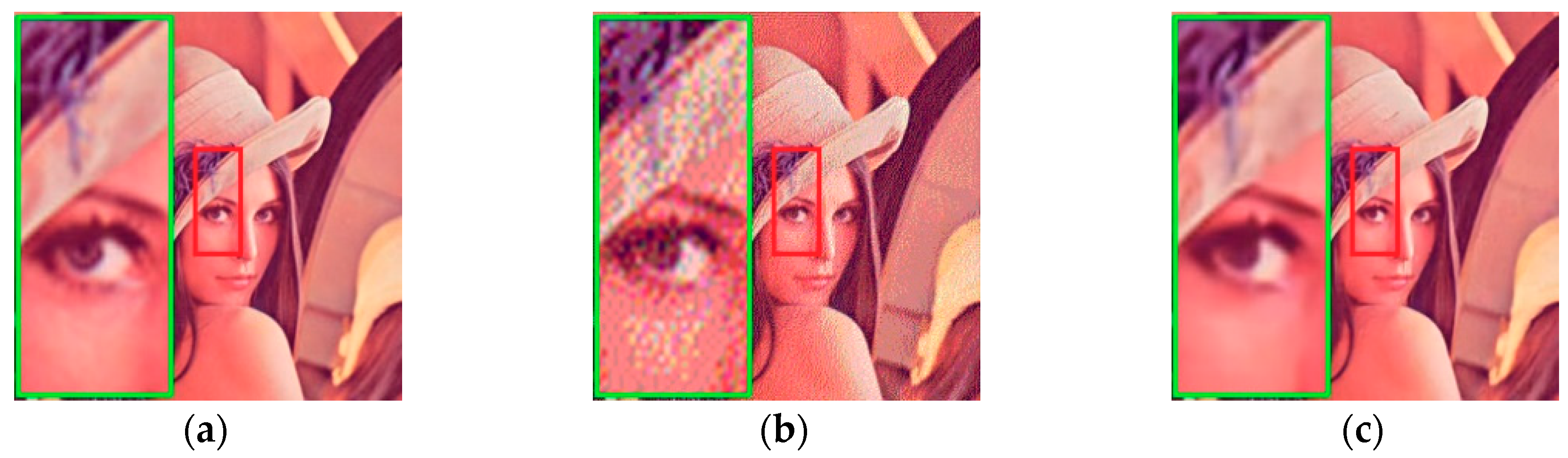
Digital halftoning is a special image transformation technology that can convert continuous-tone images into halftone images with only 1 bit per pixel. Different from the general binary image, the halftone image can be perceived as a continuous-tone image when it is viewed from a certain distance because of the low filtering character of the human visual system. Halftone images are widely used in many fields, such as the printing industry [1], telemedicine [2], Internet of Things (IoT) [3], and the textile industry [4]. The common application case of halftone image is for bi-level output devices such as printing press, printers, copiers, fax machines, plasma display panels, and so on. Another application field is in that the halftone image can be used as an image compression mode where there is not enough storage space and ultra-low power image acquisition is needed, such as in telemedicine and IoT [2,3]. Inverse halftoning is an inverse process of halftoning that is used to restore continuous-tone images from their halftone versions. This inverse process is needed because typical image processing techniques are suitable to continuous-tone images but are very difficult to halftone images. Nowadays, inverse halftoning is required in many practical applications, such as image compression, image restoration, watermarking, high dynamic range imaging, and so on. Specifically, halftone images printed in newspapers, magazines, or books are often copied by photographing or scanning for further applications, and these copied halftone images with halftone dot noises and Moiré artifacts need to be restored as clear and high quality continuous-tone images. Figure 1 gives an illustration of halftoning and inverse halftoning, where the halftone image in Figure 1b is generated from Figure 1a using the error diffusion digital halftoning method, and the image in Figure 1c is restored from Figue 1b by our designed inverse halftoning method. In this section, we briefly introduce halftoning and inverse halftoning technologies.
1.1. Halftoning Technology
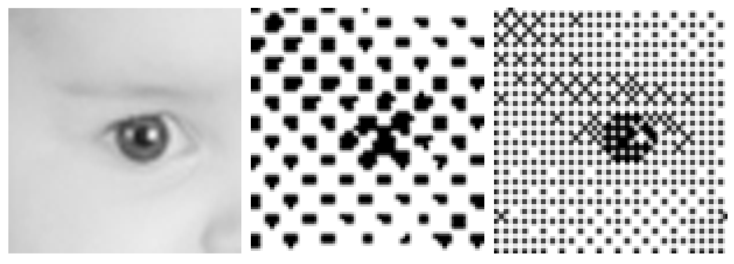
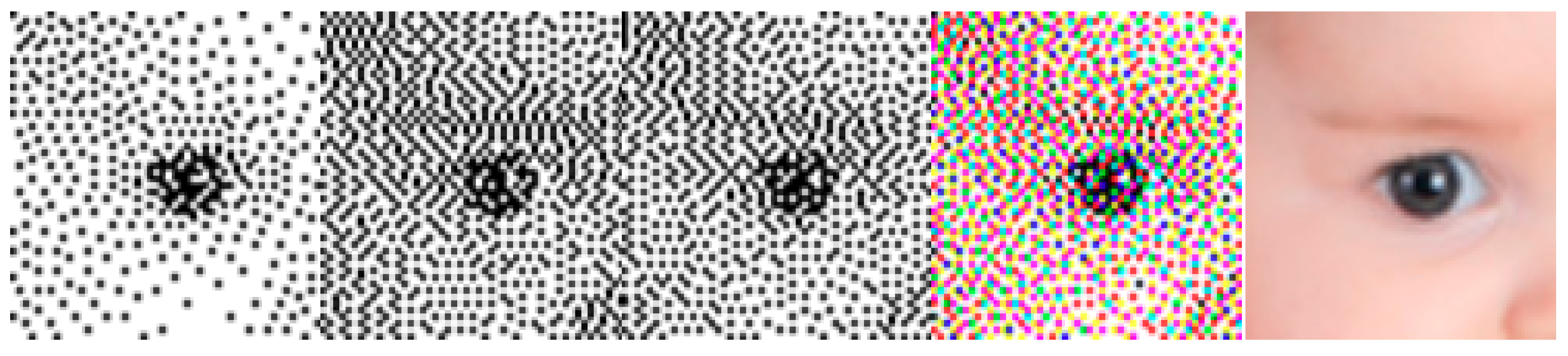
Digital halftoning is a technique that simulates continuous-tone images by using dots of a limited number of colors and varying dots either in size or in spacing. According to the distribution of dots, it can be divided into amplitude-modulated (AM) screening and frequency-modulated (FM) screening as shown in Figure 2. The image hierarchy is represented by the size of the dots in AM screening whereas the dot distance is fixed in spacing and by the density of dots in FM screening [1]. Color halftone images refer to the overlapping halftone images generated from its each color channel. Figure 3 gives an illustration of color halftone image generated by RGB color image. If the image mode is CMYK (cyan, magenta, yellow, black), then C, M, Y, and K channel halftone processing is required instead of a R, G, and B channel image. Besides the AM and FM screening methods, a large amount of digital halftoning methods have been presented, such as ordered dithering, error diffusion, dot diffusion, iterative processing, and methods based on look-up table (LUT) [5].
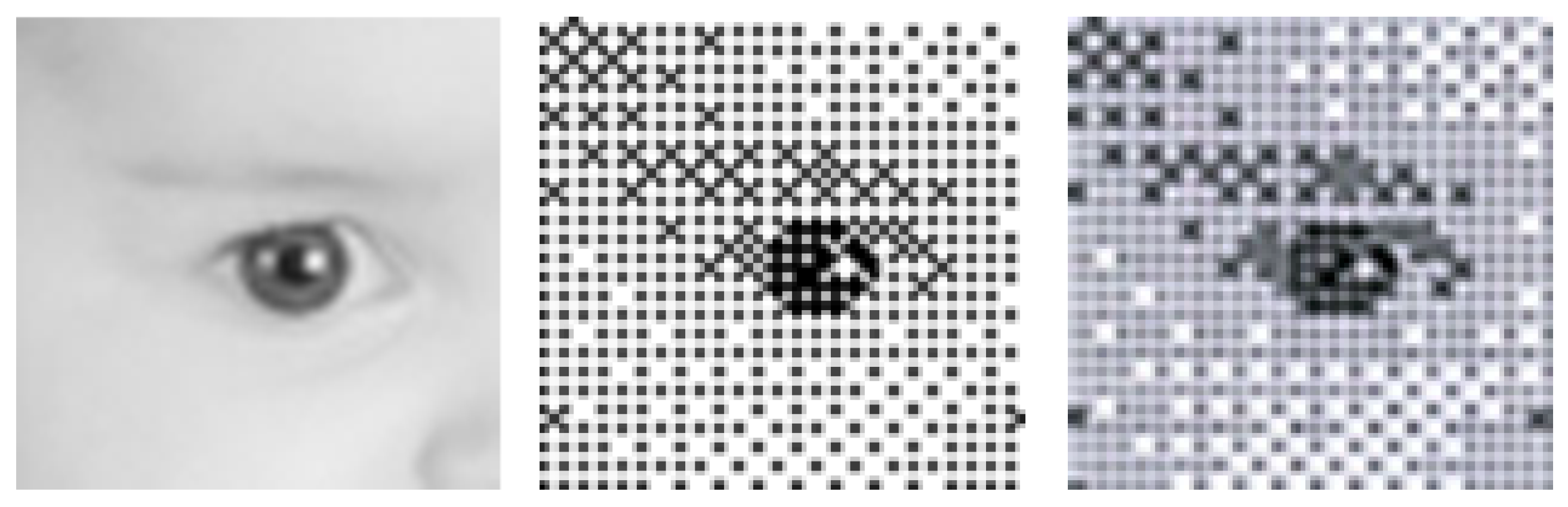
For halftone images, there are two existing forms: one is in the form of an electronic document, and the other is in the form of a printed medium such as newspapers, books or magazines. For the halftone image in the form of electronic document, we call it a digital halftone image because it does not print on analog medium, whereas for the halftone image in the form of a printed medium, we call it a scanned halftone image because it needs to be scanned into the computer first when we want to reuse it. Figure 4 shows an example of these two types of halftone images. As shown in Figure 4, the scanned halftone image is more blurred and has more serious quality degradation than the digital halftone image.
1.2. Inverse Halftoning Technology
Inverse halftoning is an ill-posed problem because of the inevitable information loss during halftoning. From Figure 2, Figure 3 and Figure 4, we can see that there are halftone noise patterns existing in both digital halftone images and scanned halftone images, and more complex quality degradation in scanned halftone images. Thus, the critical issue of inverse halftoning is not only removing halftone noise patterns but also restoring fine details from halftone images. Over the last decades, many inverse halftoning methods have been proposed, such as low-filtering methods [6,7], projection onto convex sets method (POCS) [8], maximum a posteriori (MAP) estimation method [9], wavelet-based method [10], look-up-table method (LUT) [11,12], dictionary learning method [13,14], and neural networks method [15]. The references [1] and [16] reviewed these methods in detail. Although these traditional methods achieved state-of-the-art performance at that time, the restored continuous-tone images still suffer from visual artifacts and subtle details loss. Hence, inverse halftoning is still a promising but challenging problem.
Recently, deep convolution neural networks (DCNN) have demonstrated their powerful ability in many image processing tasks. As a result, more and more researchers are focusing on inverse halftoning based on DCNN [17,18,19,20,21,22,23,24,25,26,27,28,29,30]. In particular, the first work using deep learning for inverse halftoning was presented by Hou and Qiu [17]. To promote the research of inverse halftoning, we reviewed the recently development of inverse halftoning method based on deep learning. Because complex and compounded degradation processes exist for scanned halftone images, such as ink smear, paper fiber structures, and paper damage with time, and there are no paired real data for learning [24], the inverse halftoning method for scanned halftone images is different from that for digital halftone images. Thus, the review on inverse halftoning based on deep learning is arranged in terms of following the two directions of digital halftone images and scanned halftone images.
The remainder of the paper is organized as follows. Section 2 introduces the inverse halftoning method for digital halftone images. Accordingly, the inverse halftone method for scanned halftone images is investigated in Section 3. Section 4 presents and discusses the existing image quality evaluations through experiments, and the prospects are drawn in Section 5. Section 6 provides a summary.
2. Inverse Halftoning Technology for Digital Halftoning
Inverse halftoning for digital halftone images can be considered as a nonlinear transformation from a halftone image to a continuous-tone image, which can be expressed as follows:
where and refer to the digital halftoning image and the restored continuous-tone image by inverse halftoning method, respectively, and represents the nonlinear transformation. Here, the DCNN is used as a nonlinear mapping function.
According to the network architecture, inverse halftoning methods for digital halftoning can be divided into two types: end-to-end learning method based on a single network (EEBSN) and end-to-end learning method based on multiple sub-networks training (EEBMN).
2.1. End-to-End Learning Method Based on A Single Network (EEBSN)
EEBSN means that the whole deep neural network consists of only one network. The specific process of EEBSN is to design the network structure, generate the training dataset, and input the dataset into the network for training.
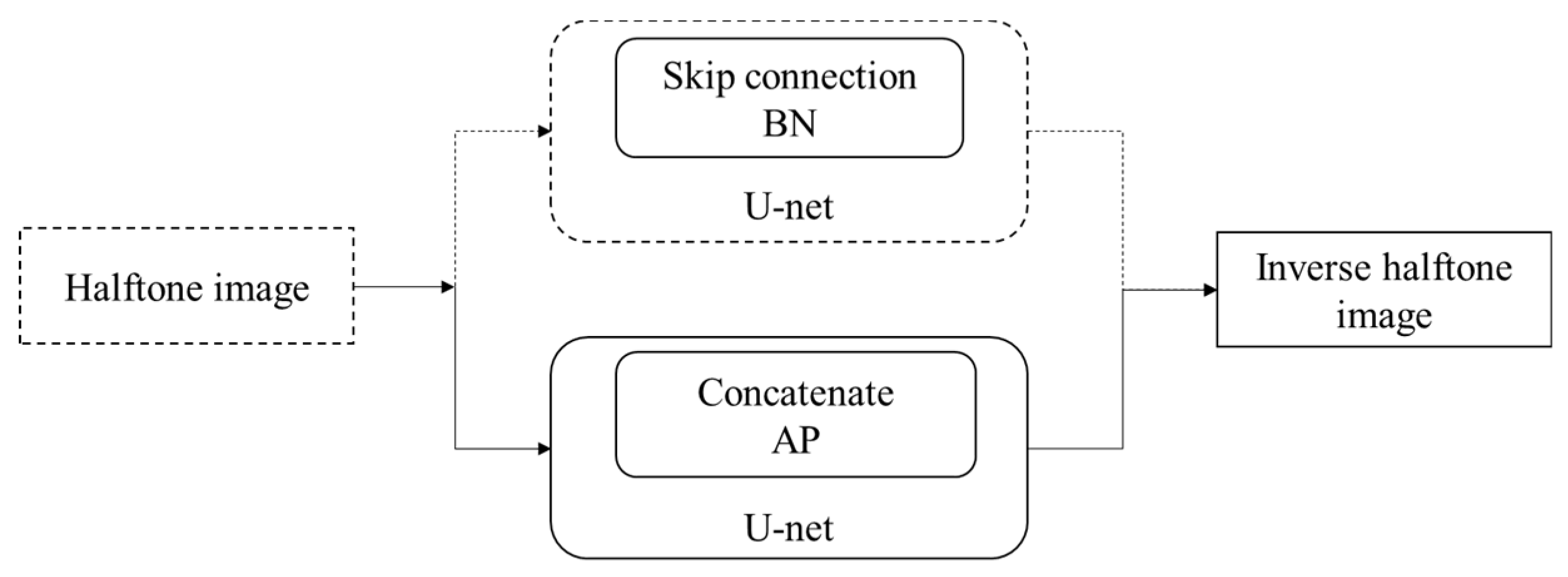
In 2017, Xianxu Hou et al. [17] first proposed an Inverse Halftoning Method based on UNet (called IH-UNet). The network structure is shown in Figure 5, where the U-Net structure combined with batch normalization (BN) were applied as the basic network structure. In order to merge the low-level features into the high-level features, the skip connection structure was added on the basis of U-Net. Following this, the U-Net structure was also used by Xiao et al. in reference [18], in which the equal-size feature graph in up-sampling and down-sampling were fused by a concatenating method instead of using skip connection, and average pooling (AP) was used for down-sampling as shown in Figure 5. Apart from the U-Net structure, the fully convolution neural network proposed in reference [19] can also be used for inverse halftoning, which consists of two types of layers: the convolution layers and Rectified Linear Unit (ReLU) layers, where they are arranged in a sequence. On the basis of the above basic principle of image transformation with DCNN, we think the ResNet proposed by He, K. et al. [31] and the DenseNet proposed by Huang, G. et al. [32] can also be taken as a basic network structure for inverse halftoning.
The loss function is another important problem for inverse halftoning based on DCNN. The common loss function used in reference [18] was the mean square error (MSE) of the restored continuous-tone image and its corresponding real continuous-tone image , which is a per-pixel loss function as follows:
where is the pixel number of image or image .
Due to easy producing blurry outputs or visual artifacts by per-pixel losses, the perceptual loss was used in reference [17], which was used to measure the difference between two images at different deep feature levels on the basis of pre-trained deep convolutional neural networks. The perceptual loss function is defined as Equation (3).
where represents the extracted features at the convolutional layer of the pre-trained deep convolutional neural network. The VGG-Net [33] is commonly used as a typical pre-trained deep convolutional neural network.
By analyzing the above methods, we found that the method in [17] was better than other methods based on a single network. The advantage of this method is that using U-Net structure and skip connection can incorporate low level features in the decoding process. In addition, the perceptual loss is a good choice for improving the quality of restored images. However, the image details are still not satisfactory.
2.2. End-to-End Learning Method Based on Training of Multiple Sub-Networks (EEBMN)
Because there are two tasks of removing halftone noise dots and restoring fine details in inverse halftoning, the mapping from halftoning images to continuous-tone images is a complex nonlinear transformation. Thus, it is difficult for inverse halftoning with a signal network to address these two tasks well. On the basis of the idea that the transformation can be considered as a compound of multiple nonlinear transformations, many researchers proposed inverse halftoning methods based on multiple sub-networks, where each sub-network was designed for a different task [19,20,21,22,23]. Depending on whether the subnetwork is pre-trained or not, the methods in references [20] are called deep learning without pre-training (DLOPT), whereas the other methods in references [19,20,21,22,23] are called deep learning with pre-training (DLWPT). Experiments show that these methods can achieve better performance than the method with a single network.
2.2.1. Deep Learning Without Pre-Training (DLOPT)
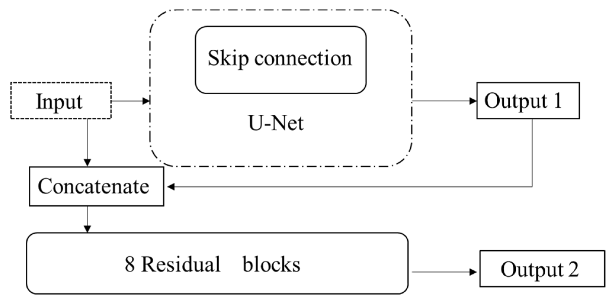
In reference [20], the authors proposed a Progressively Residual Learning network (called PRL method) which can synthesize the global tone and subtle details in a progressive manner. It consists of two modules: content aggregation module and detail enhancement module. The network architecture is briefly depicted in Figure 6. For the content aggregation, the sub-network looks like a U-Net structure with skip connection. It starts with a convolutional layer and a residual block, followed by two downscaling blocks, and then four residual blocks for constructing the content and tone features; finally, two up-scaling blocks are used to make the feature maps back to the input resolution. For the detail enhancement module, the output of the content aggregation module and the input halftone image are concatenated and then fed into the detail enhancement module. The detail enhancement module consists of eight residual blocks, which are used to extract structural details. For the loss function, the MSE and perceptual loss are both adopted to guide the image recovery. The advantage of the method in [20] is that the image details are restored in a progressive manner, as well as the application of residual learning for extracting structural details. However, halftone dot noises still exist when it is used to restore historical photos.
2.2.2. Deep Learning with Pre-Training (DLWPT)
In order to further improve the accuracy of information reproduction, the researchers put forward the idea of firstly pre-training a network layer by layer and then training comprehensively. The process could be divided into designing the network, generating datasets according to the functions of sub-networks, pre-training the sub-network, and training the whole network in sequence.
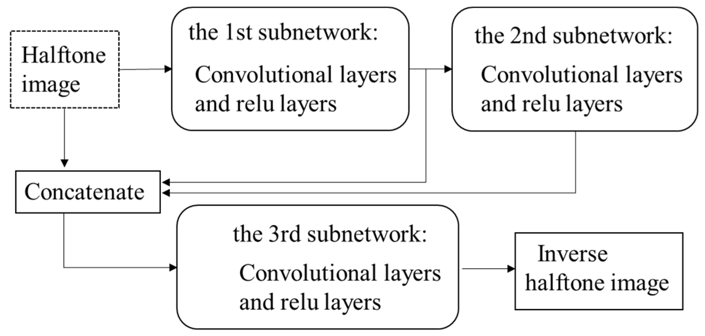
Chang-Hwan Son [19] proposed an inverse halftoning method through structure-aware DCNN, with the network being composed of three sub-networks as shown in Figure 7, in which each sub-network is constructed by a different number of layers including convolution and ReLU operation. The first sub-network aims to generate the initial continuous-tone image from an input halftone image, whereas the second sub-network connected to the output of the first sub-network is designed to extract local image structures such as lines, curves, or textures. The input halftone image, the output of the first sub-network, and the second sub-network are all concatenated and then fed into the third sub-network for reconstructing the final continuous-tone image. As shown in Figure 7, the entire network is trained in stages with each sub-network. The first sub-network is primarily trained using the input halftone and its corresponding continuous-tone image, where the MSE loss function is employed to guide the training process. Once the first sub-network has been trained well, the second sub-network begins to be trained. For the training of the second sub-network, the Sobel gradient operator is applied to generate the gradient image, and the MSE loss between the gradient images generated by the output of the second sub-network and the original continuous-tone image is used to train it. Ultimately, the halftone images and continuous-tone images are applied to train the whole network, including the third sub-network in an end-to-end manner. The advantage of this method is that the image structure map predictor (ISMP) is introduced in the network, which can predict image structure for improving the quality of restored images. The disadvantage of the method is that the experiment is only evaluated in halftone images generated by the error diffusion method.
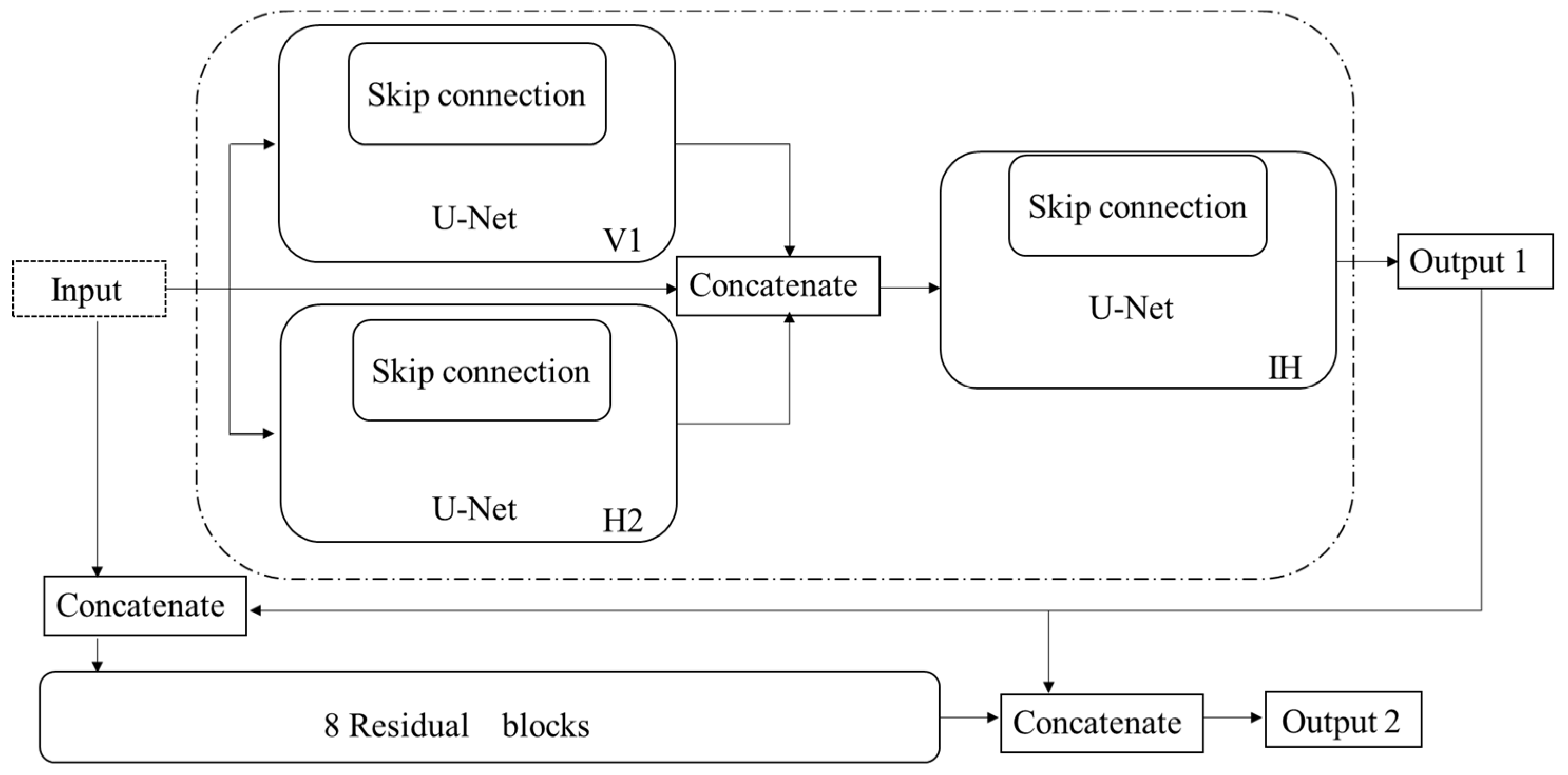
The same as reference [19], Xiao et al. [21] also used gradient information in their proposed network to boost details in the recovered continuous-tone image. In contrast to the method in reference [19], the proposed network as shown in the dashed box of Figure 8 firstly extracts the vertical and horizontal gradient information directly from the input halftone image by sub-network V1 and sub-network V2, respectively. Then, the input halftone image and two gradient maps generated by the sub-network V1 and sub-network V2 are concatenated as the input of the third sub-network IH. The third sub-network IH is used to restore continuous-tone images. All the three sub-networks have the same architecture with a U-shaped encoder–decoder and skip connections. The training of the network is divided into two stages. In the first stage, the sub-network V1 and V2 are pre-trained, respectively, by the MSE loss between gradient maps obtained from ground truth images and predicated gradient maps generated by the sub-network V1 and V2. In the second stage, the loss function for training the third sub-network IH is composed of two parts: the first part is the MSE loss between the final output image and the ground truth image, and the second part is the gradient loss term.
To further enhance the detail and texture information, Yuan et al. [22] proposed an improved method based on the method in the reference [21], which takes the effectiveness of residual sub-network into account, as shown in Figure 8. For the training of the residual sub-network, the loss between the predicted continuous-tone image by the residual sub-network and the ground truth image is used. To make the residual sub-network and the sub-network composed by V1, V2, and IH collaborate more seamless, the pixel value loss and the gradient loss are combined to fine-tune the parameters of two networks. Compared with the method in [21], the advantage of [22] is the introducing of the gradient guided block and residual learning model, which are beneficial in enhancing the fine image details. Nevertheless, some noise patterns in restored images still exist.
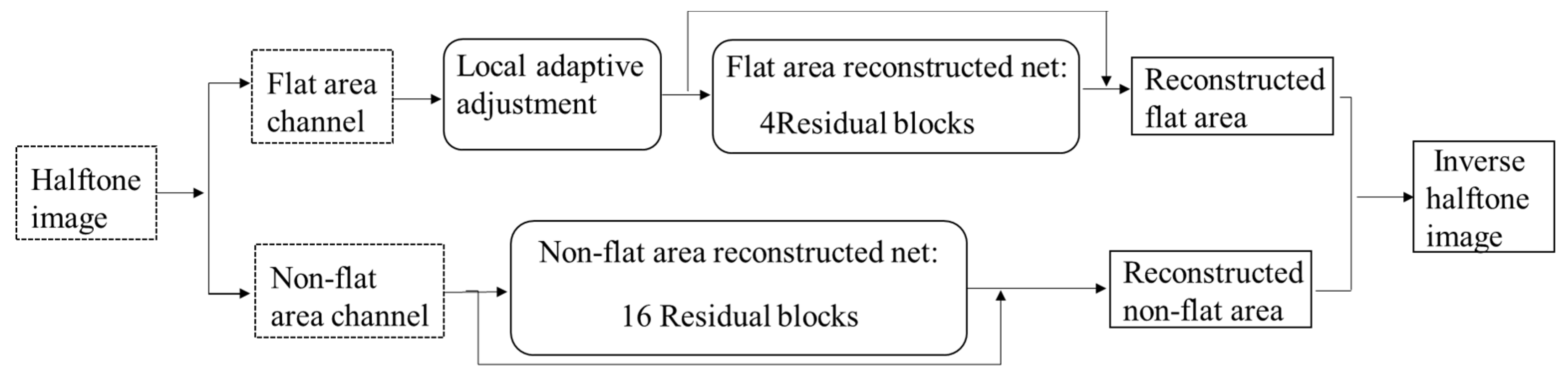
Considering the restoration of non-smooth areas such as texture and details will affect the reproduction of smooth areas in a single network. Zhao et al. [23] proposed an opposite method that restores smooth area prior to restoring details. The network architecture is shown in Figure 9. Firstly, the halftone image is divided into flat area and non-flat area. Then, the pre-trained local adaptive adjustment method is used to smooth the flat area and the residual blocks are adopted to further construct the smooth area. The residual blocks consist of two convolutional layers, two batch normalizations, and ReLU. The non-flat area channel is restored by applying residual blocks alone. Finally, the reconstructed flat area and non-flat area are combined to generate an inverse halftone image. The method in reference [23] is proposed for bit-depth expansion and obtains favorable visual quality, but the halftone dot noises cannot be removed clean because the objective of this method is not designed for inverse halftoning.
3. Inverse Halftoning Technology for Scanned Halftone Images
The inverse halftoning method for scanned halftone images refers to converting the scanned halftone image into a continuous-tone image. This method is used to preserve valuable works of art in electronic form, such as ancient books, calligraphy, and paintings. Due to some obvious quality reduction in the scanned halftone image, such as dot deformation, ink smear, and paper changes with time, the restoring of the scanned halftone image is more complex compared to the digital halftone image. In addition, there is no paired real data for scanned halftone images. Thus, the means of restoring a high quality continuous-tone image from a scanned halftone image is a challenging process.
Fundamentally, inverse halftoning is an image restoration problem. Thus, some general purpose DCNNs for image restoration can also be used for inverse halftoning, such as super-resolution networks, style transfer networks, and Generative Adversarial Networks (GANs). In this section, according to whether the network is specially designed for inverse scanned halftone images, the inverse halftoning method for scanned halftone images is divided into two types: the method based on general purpose DCNNs and the method for specially designed DCNNs.
3.1. Inverse Halftoning Based on General Purpose DCNNs for Scanned Halftone Images
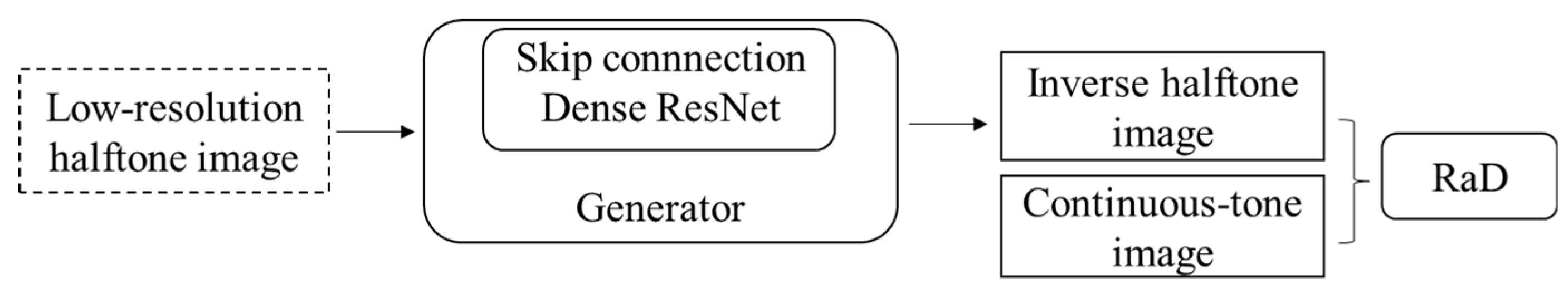
Super-resolution reconstruction is a typical image processing problem that is used to restore high resolution images from low resolution images. Similarly, inverse halftoning can also be considered as an image super-resolution reconstruction problem. Thus, the DCNN designed for super-resolution reconstruction can also be used for inverse halftoning. In reference [24], the authors Gao et al. used the Enhanced Super-Resolution Generative Adversarial Networks (ESRGAN method) proposed by Wu et al. [25] for comparison with their proposed inverse halftoning method. The architecture of ESRGAN is shown in Figure 10, which is the optimized version of Super-Resolution Generative Adversarial Network (SRGAN) [34]. In ESRGAN, the discriminator of Relativistic GAN (RaGAN) [35] and dense block [32] are adopted to replace the discriminator of SRGAN and residual block [31], and the batch normalization is also removed.
Image style transfer is a technique that converts an image into another style image. On the basis of the idea that halftone images and continuous-tone images are two different style images, the DCNN designed for style transfer can be retrained for inverse halftoning. Considering the limitations of no paired dataset for scanned halftone images, DCNNs based on unsupervised GAN network proposed by Ian Goodfellow [36] is a better choice, such as CycleGAN [26] and XNet [27].
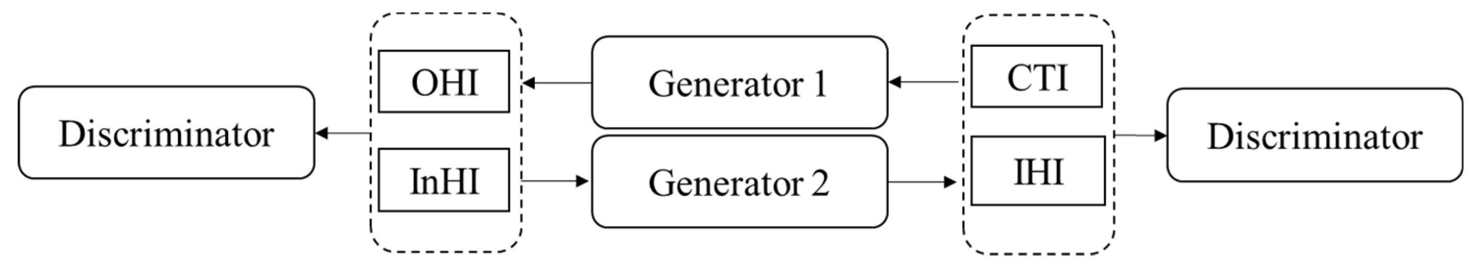
The core technique of CycleGAN is the two mapping generators, with which the whole process can be performed as a loop as shown in Figure 11. The two mapping generators denote the generator of converting halftone images to inverse halftone images and the generator of transferring continuous-tone images to halftone images. Meanwhile, two discriminators are used to promote the generation of the optimal inverse halftone image. One is used to reduce the difference between the generated halftone image and the original halftone image, and the other is used to narrow the gap between the inverse halftone image and the continuous-tone image. The cycle structure with two discriminators realizes the conversion of halftone and continuous-tone style smoothly.
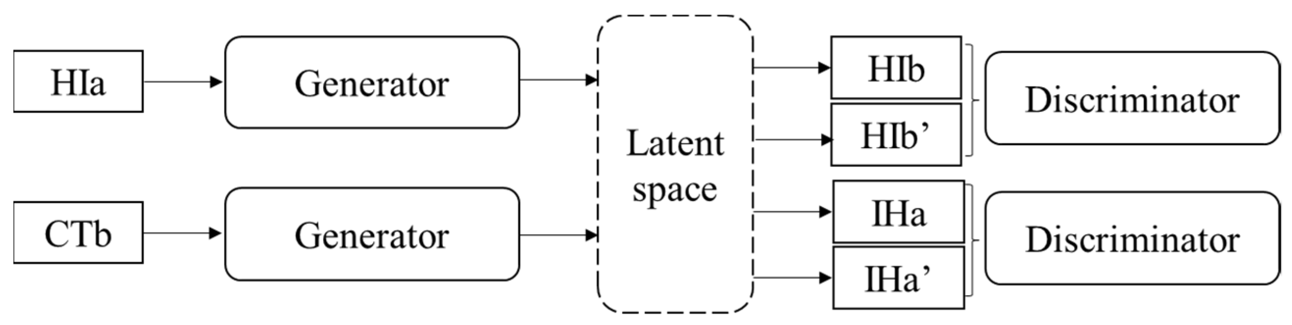
In 2019, Omry Sendik [27] proposed the concept of latent space on the basis of CycleGAN, and designed XNet by fusing two common GAN networks as shown in Figure 12. Accordingly, cross identity loss, latent cycle-consistency loss, and latent cross-translation consistency loss were proposed, which are similar to the principle in CycleGAN. These loss functions make constraints on training more accurate and are prone to achieving better performance.
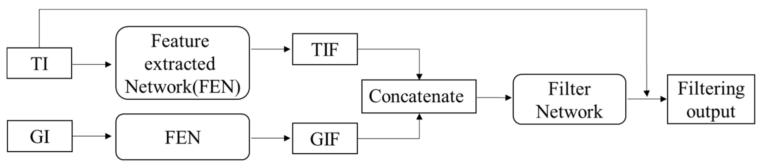
To sum up, the GAN-based network can indeed be applied to inverse halftoning, but the image performance is not ideal because of the uncertainty of information learning. To alleviate the problem, Li et al. [28] proposed a phased inverse halftoning method, as shown in Figure 13, which consists of three sub-networks with a three-layer. The whole process is divided into dataset generation and network training. For dataset generation, the rough image and guidance image are generated by processing the scanned halftone image with previous methods. For network training, the training dataset is firstly sent to the first two sub-networks for feature extraction, and then the extracted features are inputted into the filter network. The smaller the residual, the closer the restored image and original continuous-tone image will be. Although the above general purpose DCNN methods can be retrained for inverse halftoning, the restored image quality is poor compared with those of purposefully designed inverse haltoning.
3.2. Inverse Halftoning Based on Special Designed DCNNs for Scanned Halftone Images
During the process of printing and scanning, the scanned halftone image quality is seriously degraded, and there is no paired real data for machining learning. Thus, the inverse halftoning for scanned halftone images is more difficult than the method for the digital halftone image. None of the existing DCNN methods can satisfy for scanned halftone images. Recently, only a few studies have addressed this problem, such as in references [24,29,30], where the DCNN is specially designed for inverting scanned halftone images.
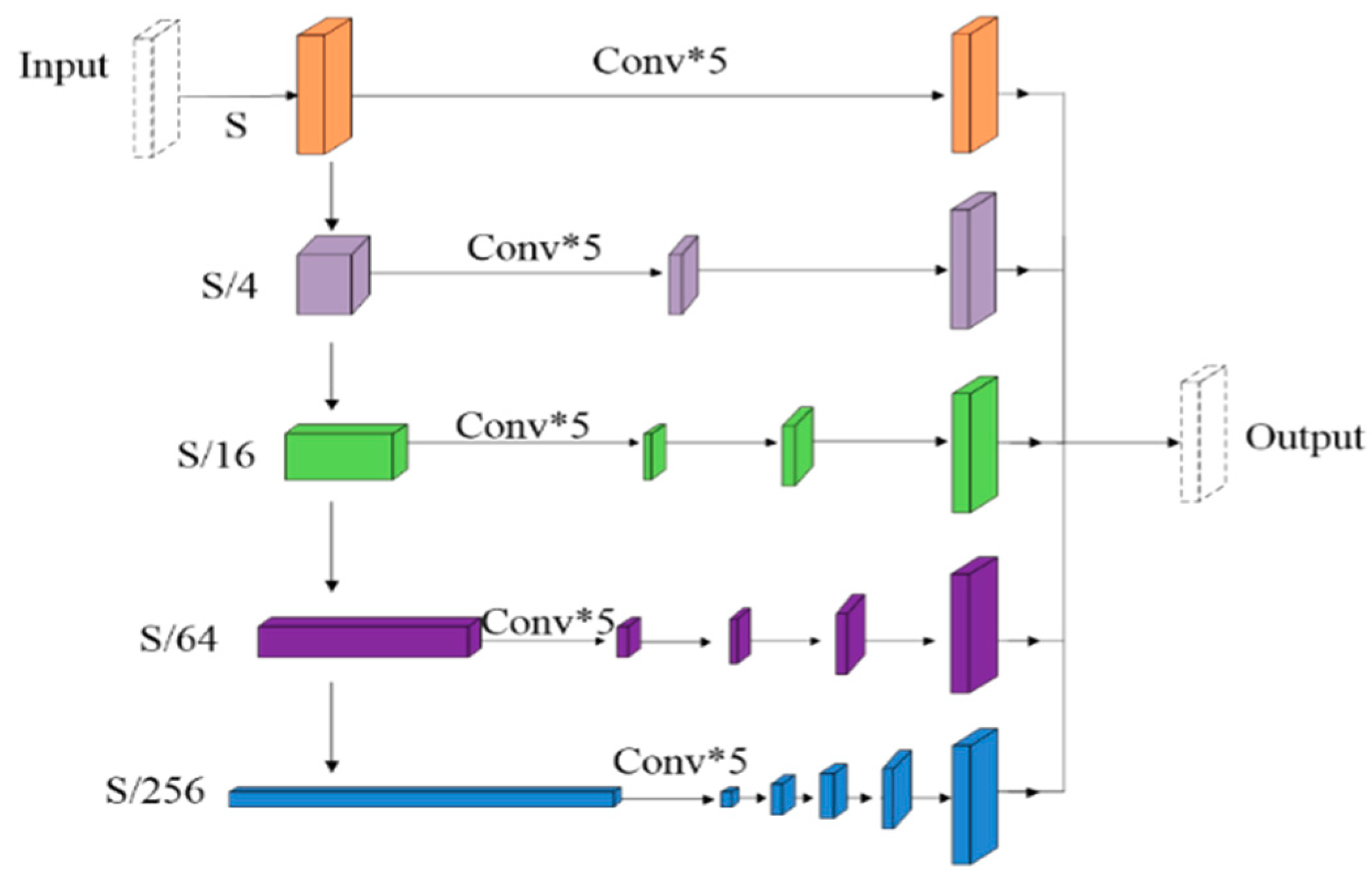
In terms of scanned halftone images, they are often contaminated with moiré patterns. Considering the moiré patterns span over a wide range of frequencies, Sun et al. [29] proposed a multi-resolution DCNN for moiré pattern removal. The proposed architecture is shown in Figure 14, in which the input image is firstly converted into multiple feature maps at different resolution levels by a nonlinear multi-resolution analysis, and then each feature map is fed into a sequence of cascaded convolutional layers for removing the moiré pattern associated with the specific frequency band of this branch, and finally the outputs at different resolutions are up-sampled as the input resolution and fused together as the final output image. The method of the reference [29] is a groundbreaking work for moiré pattern removal, which achieved the state-of-the-art performance in this field at that time. However, there is still room for improving image details.
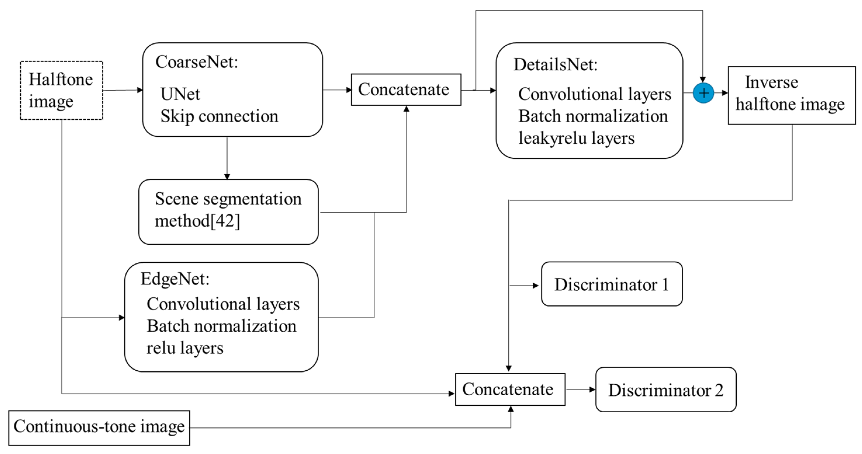
Another famous work is the research proposed in reference [30], which can not only remove halftone artifacts but also synthesize the fine details lost during halftone. The network is depicted as shown in Figure 15, which combines the GAN network with other networks, such as semantic segmentation network [37] and U-Net [38]. The method consists of two stages. In the first stage, the initial inverse halftone image is generated by applying CoarseNet, semantic segmentation network [37], and EdgeNet rationally. CoarseNet, which consists of U-Net and skip connection, is used to reconstruct colors, tones, and shapes roughly. The semantic segmentation network [37] is adopted to generate object-level context and extract edge information by the EdgeNet. In the second stage, the DetailsNet, which also consists of common convolutional layer, is used to enhance details and further remove artifacts in images. To improve the quality of the inverse halftone image, two discriminators [39] were adopted, where one is used to detect the whole image while the other is to examine local regions. Compared to previous methods, the proposed method can achieve more convincing results, but this is dependent on the training examples.
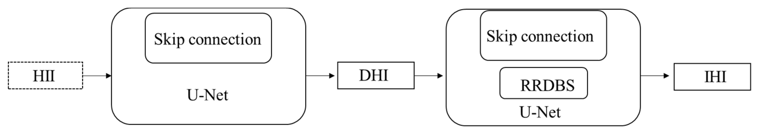
Aiming at the restoration of invaluable historical photographs in the form of halftone prints in old publications, Gao et al. [24] proposed a pioneering method to address this issue. The challenge is that the quality of the scanned halftone image is poor and no paired real data are available for training. To solve these problems, the authors [24] developed a novel learning strategy by dividing the task into two stages as shown in Figure 16. The first stage is to remove printing artifacts, where the scanned halftone image is transformed to a digital halftone image. Due to lack of paired data, the CycleGAN technique is employed in the sub-network used in the first stage, which is an unsupervised learning network including U-Net structure and skip connection. Through the first stage, the scanned halftone image is converted into a synthetic halftone image. In the second stage, the synthetic halftone image can be converted into a continuous-tone image by inverse halftoning method for digital halftone images. Because sufficient paired images can be easily generated by using the halftone synthesizer, the sub-network used in the second stage is easily trained. The sub-network in the second stage is composed of U-Net structure, skip connection, and Residual-in-Residual Dense Blocks (RRDBS) 32]. The advantage of this method is that it does not need paired data in the first stage, whereas the second stage can be easily trained with synthetic data. However, it fails to input halftone prints with severely damaged areas.
4. Quality Evaluations of Inverse Halftone Images
To evaluate the performance of various inverse halftoning methods, the corresponding image evaluation methods are studied in this section, which are divided into subjective evaluation and objective evaluation. The subjective evaluation is mainly based on human eyes, which will be affected by people’s national characteristics, customs, and cultural background. The objective evaluation is a quantitative method, which can cover the shortage of subjective evaluation. In this section, some typical inverse halftoning methods based on deep learning, such as PRL [20], IH-UNet [17], and ESRGAN [25] networks, are evaluated on the basis of the evaluation index.
4.1. Subjective Evaluation
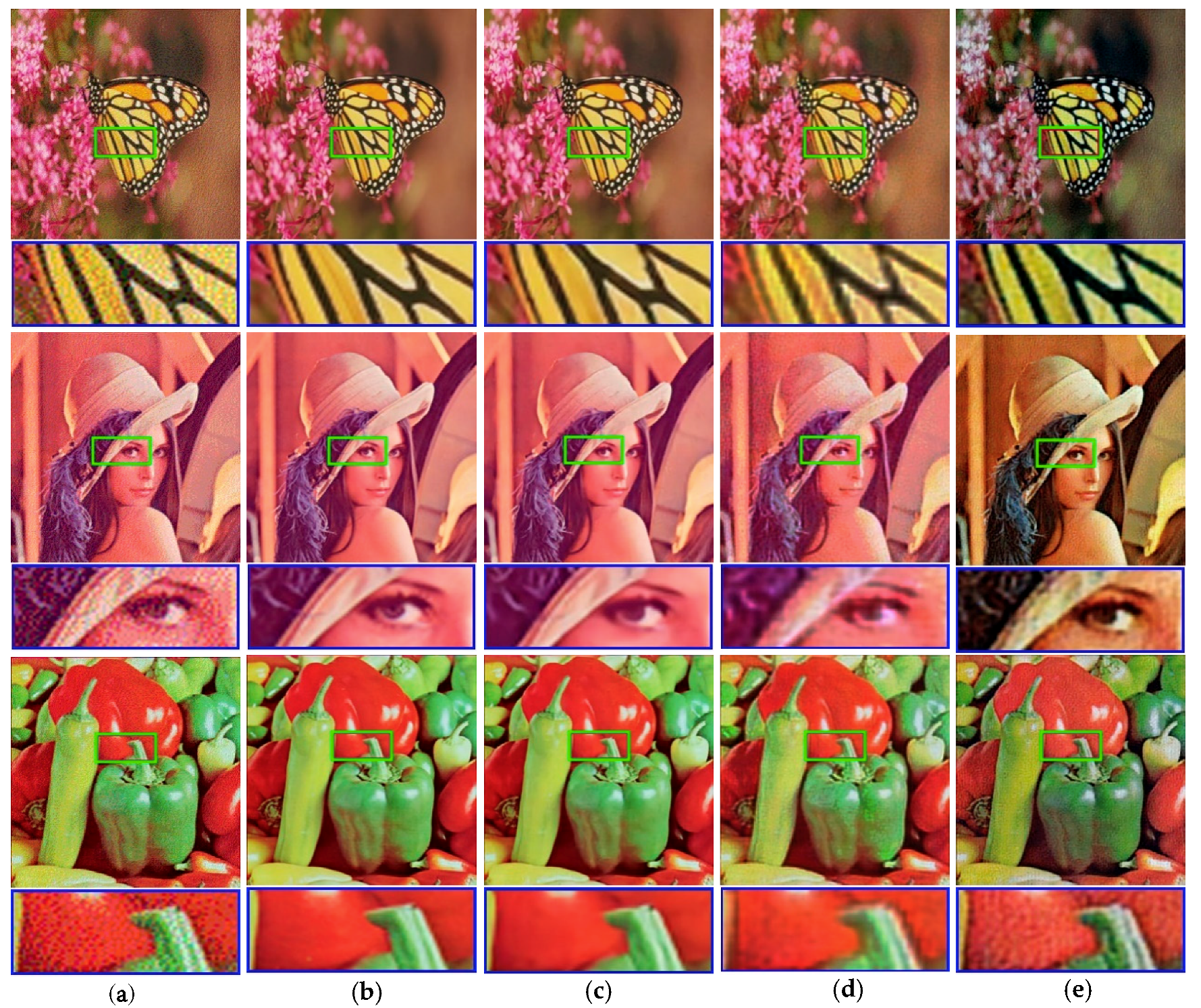
Subjective evaluation is the most commonly used and direct method, which is to judge and evaluate images by observers according to their experience or specified evaluation scale [40]. The restored continuous-tone image is evaluated by considering the following factors: halftone dot noise removal, texture detail reproduction, smooth area processing, and chromatic aberration. As shown in Figure 17, the continuous-tone images restored by the IH-UNet [17] and PRL method [20] are better in dot removal than others, whereas the images processed by the PRL method perform better in the smooth region. In terms of texture details, the image processed by ESRGAN [25] is the clearest, whereas the images processed by PRL is the closest to the original continuous-tone image. In the aspect of color reproducing, the image generated by the PRL method is the most similar to the original image, followed by IH-UNet and ESRGAN.
4.2. Objective Evaluation
The most common used index of objective evaluation includes mean-square error (MSE), peak signal-to-noise ratio (PSNR), and structural similarity index (SSIM) [41]. Besides these indexes, the color and clarity indexes are also introduced in this subsection.
MSE is one of the most basic image quality evaluation indexes that can quantitatively evaluate the overall performance of inverse halftone images. It is a per-pixel comparison between the restored continuous-tone image and the original continuous-tone image , which is defined as follows.
where is the pixel position, and and refer to the width and height of the image, respectively.
PSNR is another commonly used image quality evaluation index. Recently, it has been widely used in the quality evaluation of inverse halftone image, focusing on the evaluation of image structure consistency. Theoretically, the higher the PSNR value, the less distortion of the inverse halftone image and the more similar the structure is to the original image. The specific expression is as follows.
SSIM is known as a perceptual-aware method for measuring the similarity between two images, and the expression of SSIM is shown as follows.
where and refer to the mean pixel values of the original continuous-tone image and the inverse halftone image, acting as brightness estimates. and refer to the pixel value variance of the original continuous-tone image and the inverse halftone image, acting as contrast estimation. refers to the covariance of the pixel values of the original continuous-tone image and the inverse halftone image, acting as a measure of the structural similarity. and are two constants for maintaining stability. The SSIM value ranges from 0 to 1, and the closer SSIM is to 1, the more similar the two images.
For color halftone image, the color difference can objectively represent the color similarity between the original image and the inverse halftone image. In 2016, Pedro et al. [42] applied color difference to evaluate the quality of inverse color halftone image. Firstly, the image values in RGB color space are converted to the relative values in CIELAB color space. Then, the color difference between images is calculated as follows.
where , , and refer to the difference in color shades and hues between inverse halftone image and the original continuous-tone image, respectively. The smaller the color difference, the more similar the inverse halftone image is to the original continuous-tone image.
It is well known that the human eyes perceive two images as being less different when the color tone changes analogously. However, the previous image quality evaluation methods did not take this into account, and only evaluated the image quality from the pixel level. To make up for this deficiency, Jin, Z. et al. [43] proposed a new color image quality evaluation index D. The smaller the value of D, the more similar the tone changes of the inverse halftone image and the original image.
where refers to the relative standard deviation of the pixel value difference between the continuous-tone image and the inverse halftone image, and refers to the relative standard deviation calculated by pixel values of the continuous-tone image.
To evaluate the performance of restoring image details of different inverse methods, the index of image clarity is employed to address this problem. The clarity is the internal evaluation method of the image, independent of the original image. The higher the clarity, the clearer the details in the image will be. The clarity is defined as follows.
Finally, we evaluated the image quality on the basis of the above indexes in order to compare the different inverse halftoning methods. The experimental images include the butterfly image, the Lena image, and the peppers image, and the halftone images were generated by the error diffusion method. The inverse halftoning method consists of the PRL method [20], the IH-UNet method [17], and the ESRGAN method [25]. Table 1 gives the experimental results. As shown in Table 1, all objective evaluation indexes can show the image quality in corresponding aspects, which are consistent with the visual performance effect, and all have reference significance. However, none of them could individually evaluate image quality comprehensively. From Table 1, we can also see that the performance of the method based on multiple sub-networks (PRL method) is better than the method based on a single network (IH-UNet method), and the performance of the method based on a general purpose DCNN (ESRGAN method) is the worst.
5. Prospects
With the rapid development of digital multimedia technology and equipment, inverse halftoning technology has become an essential part of image display with high precision. Although many inverse halftoning methods have been proposed, there are still improved room for problems, such as multi-modal halftone image recovery, color image distortion, scanned halftone image recovery, and image quality evaluation.
5.1. Multi-Modal Halftone Images Recovery
The existing inverse halftoning methods are for a certain digital halftoning method, such as error diffusion method. The quality of restored continuous-tone images will degrade when they are used for another type of halftone images. In practical application, there are many different types of halftone images, which are called multi-modal halftone images. For example, there are 23 types of halftone images in reference [44]. Thus, the means of restoring a high quality image by taking into consideration of these multi-modal halftone images is a challenging problem. In future research, we will employ the StarGAN [45] deep model to study this problem in order to realize multi-modal inverse halftoning by one deep model.
5.2. Inverse Halftoning Technology for Color Image Distortion
The existing color inverse halftoning technology is to obtain the inverse halftone image through the inverse halftone processing of each channel, resulting in poor visual quality in color performance. Therefore, to construct the relationship between the color channel and the specific color space model is an important aspect of the research on color image inverse halftoning. To address this issue, we can add color difference information between the restored continuous-tone image and the original continuous-tone image into the loss function. On the other hand, we can add a sub-network to restore the color information. The experimental results of the method in reference [20] demonstrated that networks at different stages tend to recover different aspects of image information. On the basis of this idea, in the following study we will design a deep network with three sub-networks. The first sub-network is employed to remove halftone noises and restore the initial continuous-tone image, the second sub-network is designed to enhance detail and texture information, and the last sub-network is applied to adjust color performance. At the same time, the corresponding loss functions will be set for each sub-network and the whole deep network, in which color difference loss function will be considered emphatically.
5.3. Adaptive Inverse Halftoning for Scanned Halftone Images
Generally, there is no paired images for scanned halftone images, and quality degradation exists during the process of printing and scanning, especially for old halftone images printed on newspapers or books. Nowadays, few researchers study this problem, except for the studies [24,30]. However, some scanned halftone images with severe blemishes will fail to be restored. In addition, the question of scanned halftone images with different scanned resolution has not been investigated. Therefore, to construct a deep learning network that can quickly adapt to various conditions so as to obtain high quality scanned inverse halftone images is urgently needed. Recently, Kim et al. [46] proposed a Halftone Color Decomposing Convolutional Neural Network (HCD-CNN) that can better decompose the photographed image or scanned image as C, M, Y, and K halftone images. Inspired by the HCD-CNN, the scanned halftone image can be firstly decomposed as CMYK images, and then inversed as a continuous-tone image using an inverse halftone method for digital halftone images.
5.4. Inverse Halftone Image Quality Evaluation
The image quality evaluation is a very effective way to judge the effectiveness of the inverse halftoning method. As mentioned in Section 4, there are many evaluation methods for inverse halftone images, but they are all generally subjective and objective evaluation methods for image quality, which are still far from the intuitive perception of human eyes. As shown in Figure 17 and Table 1, the visual effect of restored images and the objective evaluation indexes are not consistent to a certain extent. In particular, there is no effective quality evaluation for inverse halftoning images that have no original images. Therefore, a more effective and intuitive image quality evaluation method for inverse halftoning is still a problem for the immediate future.
6. Conclusions
This paper mainly reviewed the inverse halftoning methods based on deep learning and their evaluation metrics. According to the source of halftone images, the methods are classified as methods for digital halftone images and methods for scanned halftone images. Firstly, the network architecture and the loss function were discussed. It can be seen that for the supervision network, the entire inverse halftone network mainly applies the U-Net structure and skip connection or its advanced version structure to restore continuous-tone images. In addition, multiple sub-network architecture is a good choice for executing different restoring tasks. The per-pixel loss such as MSE and the perceptual loss are generally adopted as loss function to guide training. For unsupervised network, the whole network is based on GAN network, and the loss function is generally composed of generator loss and discriminator loss for GAN network, cycle consistency loss, and perception loss. Then, the evaluation index of inverse halftone image was discussed. According to the experimental results, we should use several indexes to evaluate the inverse halftone image in practice. At the end of the review, in view of the limitations of the prior inverse halftoning methods and the shortcomings of the existing evaluation index, we put forward the prospects of the future research direction.
Author Contributions
E.Z. conceived this study and improved the text of the manuscript. M.L. designed the research and wrote the manuscript. Y.W. wrote the program code. J.D. and C.J. acquired the test images and proposed some valuable suggestions. All authors have read and agreed to the published version of the manuscript.
Funding
This work is supported by the Key Program of Natural Science Foundation of Shaanxi Province of China under grant no. 2017JZ020, the National Natural Science Foundation of China under grant no. 61771386 and no. 61671374.
Conflicts of Interest
The authors declare no conflicts of interest.
References
- Zhang, F.; Zhang, X. Image inverse halftoning and descreening: A review. Multimedia Tools Appl. 2019, 78, 21021–21039. [Google Scholar] [CrossRef]
- Ashour, A.; Guo, Y.; Hawas, A.R.; Du, C. Optimised halftoning and inverse halftoning of dermoscopic images for supporting teledermoscopy system. IET Image Process. 2019, 13, 529–536. [Google Scholar] [CrossRef]
- Kodge, S.; Chaudhary, H.; Sharad, M. Low Power Image Acquisition Scheme Using On-Pixel Event Driven Halftoning. In Proceedings of the 2017 IEEE Computer Society Annual Symposium on VLSI (ISVLSI 2017), Bochum, North Rhine-Westfalia, Germany, 3–5 July 2017; pp. 260–265. [Google Scholar]
- Kang, X.; Zhang, E. A universal defect detection approach for various types of fabrics based on the Elo-rating algorithm of the integral image. Text. Res. J. 2019, 89, 4766–4793. [Google Scholar] [CrossRef]
- Zhang, Y.; Zhang, E.; Chen, W. Deep neural network for halftone image classification based on sparse auto-encoder. Eng. Appl. Artif. Intell. 2016, 50, 245–255. [Google Scholar] [CrossRef]
- Chen, L.-M.; Hang, H.-M. An adaptive inverse halftoning algorithm. IEEE Trans. Image Process. 1997, 6, 1202–1209. [Google Scholar] [CrossRef] [PubMed]
- Kite, T.; Damera-Venkata, N.; Evans, B.; Bovik, A. A fast, high-quality inverse halftoning algorithm for error diffused halftones. IEEE Trans. Image Process. 2000, 9, 1583–1592. [Google Scholar] [CrossRef] [PubMed]
- Unal, G.; Cetin, A. Restoration of error-diffused images using projection onto convex sets. IEEE Trans. Image Process. 2001, 10, 1836–1841. [Google Scholar] [CrossRef]
- Stevenson, R. Inverse halftoning via MAP estimation. IEEE Trans. Image Process. 1997, 6, 574–583. [Google Scholar] [CrossRef]
- Xiong, Z.; Orchard, M.T.; Ramchandran, K. Inverse halftoning using wavelets. IEEE Trans. Image Process. 1999, 8, 1479–1483. [Google Scholar] [CrossRef]
- Mese, M.; Vaidyanathan, P. Look-up table (LUT) method for inverse halftoning. IEEE Trans. Image Process. 2001, 10, 1566–1578. [Google Scholar] [CrossRef]
- Zhang, E.; Zhang, Y.; Duan, J. Color Inverse Halftoning Method with the Correlation of Multi-Color Components Based on Extreme Learning Machine. Appl. Sci. 2019, 9, 841. [Google Scholar] [CrossRef] [Green Version]
- Son, C.-H.; Choo, H. Local Learned Dictionaries Optimized to Edge Orientation for Inverse Halftoning. IEEE Trans. Image Process. 2014, 23, 2542–2556. [Google Scholar] [PubMed]
- Zhang, Y.; Zhang, E.; Chen, W.; Chen, Y.; Duan, J. Sparsity-based inverse halftoning via semi-coupled multi-dictionary learning and structural clustering. Eng. Appl. Artif. Intell. 2018, 72, 43–53. [Google Scholar] [CrossRef]
- Huang, W.; Su, A.; Kuo, Y. Neural network based method for image halftoning and inverse halftoning. Expert Syst. Appl. 2008, 34, 2491–2501. [Google Scholar] [CrossRef]
- Mese, M.; Vaidyanathan, P. Recent advances in digital halftoning and inverse halftoning methods. IEEE Trans. Circuits Syst. I Regul. Pap. 2002, 49, 790–805. [Google Scholar] [CrossRef]
- Hou, X.; Qiu, G. Image Companding and Inverse Halftoning using Deep Convolutional Neural Networks. arXiv 2017, arXiv:1707.00116v2. [Google Scholar]
- Xiao, Y.; Pan, C.; Zhu, X.; Jiang, H.; Zheng, Y. Deep Neural Inverse Halftoning. In Proceedings of the 7th International Conference on Virtual Reality and Visualization, ICVRV 2017, Zhengzhou, China, 21–22 October 2017; pp. 213–218. [Google Scholar]
- Son, C.-H. Inverse Halftoning through Structure-Aware Deep Convolutional Neural Networks. arXiv 2019, arXiv:1905.00637. [Google Scholar]
- Xia, M.; Wong, T.-T. Deep Inverse Halftoning via Progressively Residual Learning. In Proceedings of the 14th Asian Conference on Computer Vision, ACCV 2018, Perth, WA, Australia, 2–6 December 2018; pp. 523–539. [Google Scholar]
- Xiao, Y.; Pan, C.; Zheng, Y.; Zhu, X.; Qin, Z.; Yuan, J. Gradient-Guided DCNN for Inverse Halftoning and Image Expanding. In Proceedings of the 14th Asian Conference on Computer Vision, ACCV 2018, Perth, WA, Australia, 2–6 December 2018; pp. 207–222. [Google Scholar]
- Yuan, J.; Pan, C.; Zheng, Y.; Zhu, X.; Qin, Z.; Xiao, Y. Gradient-Guided Residual Learning for Inverse Halftoning and Image Expanding. IEEE Access 2019, 4, 1. [Google Scholar] [CrossRef]
- Zhao, Y.; Wang, R.; Jia, W.; Zuo, W.; Liu, X.; Gao, W. Deep Reconstruction of Least Significant Bits for Bit-Depth Expansion. IEEE Trans. Image Process. 2019, 28, 2847–2859. [Google Scholar] [CrossRef]
- Gao, Q.; Shu, X.; Wu, X. Deep Restoration of Vintage Photographs from canned Halftone Prints. In Proceedings of the International Conference on Computer Vision, ICCV 2019, Seoul, Korea, 27 October–2 November 2019; pp. 1–10. [Google Scholar]
- Wang, X.; Yu, K.; Wu, S.; Gu, J.; Liu, Y.; Dong, C.; Qiao, Y.; Loy, C.C. ESRGAN: Enhanced Super-Resolution Generative Adversarial Networks. In Proceedings of the 15th European Conference on Computer Vision, ECCV 2018, Munich, Germany, 8–14 September 2018; pp. 63–79. [Google Scholar]
- Zhu, J.-Y.; Park, T.; Isola, P.; Efros, A.A. Unpaired Image-to-Image Translation Using Cycle-Consistent Adversarial Networks. In Proceedings of the 16th IEEE International Conference on Computer Vision, ICCV 2017, Venice, Italy, 22–29 October 2017; pp. 2242–2251. [Google Scholar]
- Sendik, O.; Lischinski, D.; Cohen-Or, D. XNet: GAN Latent Space Constraints. arXiv 2019, arXiv:1901.04530v1. [Google Scholar]
- Li, Y.; Huang, J.-B.; Ahuja, N.; Yang, M.-H. Joint Image Filtering with Deep Convolutional Networks. IEEE Trans. Pattern Anal. Mach. Intell. 2019, 41, 1909–1923. [Google Scholar] [CrossRef] [Green Version]
- Sun, Y.; Yu, Y.; Wang, W. Moiré Photo Restoration Using Multiresolution Convolutional Neural Networks. IEEE Trans. Image Process. 2018, 27, 4160–4172. [Google Scholar] [CrossRef] [Green Version]
- Kim, T.-H.; Park, S.-I. Deep context-aware descreening and rescreening of halftone images. ACM Trans. Graph. 2018, 37, 1–12. [Google Scholar] [CrossRef]
- He, K.; Zhang, X.; Ren, S.; Sun, J. Deep Residual Learning for Image Recognition. In Proceedings of the IEEE Computer Society Conference on Computer Vision and Pattern Recognition, Las Vegas, NV, USA, 26 June–1 July 2016; pp. 770–778. [Google Scholar]
- Huang, G.; Liu, S.; Van Der Maaten, L.; Weinberger, K.Q. CondenseNet: An Efficient DenseNet Using Learned Group Convolutions. In Proceedings of the IEEE Computer Society Conference on Computer Vision and Pattern Recognition, Salt Lake City, UT, USA, 18–22 June 2018; pp. 2752–2761. [Google Scholar]
- Simonyan, K.; Zisserman, A. Very deep convolutional networks for large-scale image recognition. In Proceedings of the 3rd International Conference on Learning Representations, ICLR 2015, San Diego, CA, USA, 7–9 May 2015. [Google Scholar]
- Ledig, C.; Theis, L.; Huszar, F.; Caballero, J.; Shi, W. Photo-Realistic Single Image Super-Resolution Using a Generative Adversarial Network. In Proceedings of the 30th IEEE Conference on Computer Vision and Pattern Recognition, CVPR 2017, Honolulu, HI, USA, 21–26 July 2017; pp. 105–114. [Google Scholar]
- Jolicoeur-Martineau, A. The relativistic discriminator: A key element missing from standard gan. In Proceedings of the 7th International Conference on Learning Representations, ICLR 2019, New Orleans, LA, USA, 6–9 May 2019. [Google Scholar]
- Goodfellow Ian, J.; Pouget-Abadie, J.; Mirza, M.; Xu, B.; Warde-Farley, D.; Ozair, S.; Courville, A.; Bengio, Y. Generative adversarial nets. In Proceedings of the 28th Conference on Neural Information Processing Systems (NIPS), Montreal, CANADA, 8–13 December 2014. [Google Scholar]
- Zhou, B.; Zhao, H.; Puig, X.; Fidler, S.; Barriuso, A.; Torralba, A. Scene parsing through ADE20K dataset. In Proceedings of the 30th IEEE Conference on Computer Vision and Pattern Recognition, CVPR 2017, Honolulu, HI, USA, 21–26 July 2017; pp. 5122–5130. [Google Scholar]
- Ronneberger, O.; Fischer, P.; Brox, T. U-Net: Convolutional Networks for Biomedical Image Segmentation. In Proceedings of the 18th International Conference on Medical Image Computing and Computer-Assisted Intervention, MICCAI 2015, Munich, Germany, 5–9 October 2015; pp. 234–241. [Google Scholar]
- Sajjadi, M.S.M.; Scholkopf, B.; Hirsch, M. EnhanceNet: Single Image Super-Resolution through Automated Texture Synthesis. In Proceedings of the IEEE International Conference on Computer Vision, Venice, Italy, 22–29 October 2017; pp. 4501–4510. [Google Scholar]
- Damera-Venkata, N.; Kite, T.D.; Geisler, W.S.; Evans, B.L.; Bovik, A.C. Image quality assessment based on a degradation model. IEEE Trans. Image Process. 2000, 9, 636–650. [Google Scholar] [CrossRef] [PubMed] [Green Version]
- Kahaki, S.M.M.; Arshad, H.; Nordin, J.; Ismail, W. Geometric feature descriptor and dissimilarity-based registration of remotely sensed imagery. PLoS ONE 2018, 13, e0200676. [Google Scholar] [CrossRef] [PubMed]
- Freitas, P.G.; Farias, M.; Araújo, A.P. Enhancing inverse halftoning via coupled dictionary training. Signal Process. Image Commun. 2016, 49, 1–8. [Google Scholar] [CrossRef]
- Jin, Z.; Fang, E. Print inverse halftoning and its quality assessment techniques. In Proceedings of the 49th Conference of the International Circle of Education Institutes for Graphic Arts Technology, Beijing, China, 14–16 May 2017; pp. 211–220. [Google Scholar]
- Guo, J.M.; Sankarasrinivasan, S. Digital Halftone Database (DHD): A Comprehensive Analysis on Halftone Types. In Proceedings of the 10th Asia-Pacific Signal and Information Processing Association Annual Summit and Conference, APSIPA ASC 2018, Honolulu, HI, USA, 12–15 November 2018; pp. 1091–1099. [Google Scholar]
- Choi, Y.; Choi, M.; Kim, M.; Ha, J.W.; Kim, S.; Choo, J. StarGAN: Unified Generative Adversarial Networks for Multi-domain Image-to-Image Translation. In Proceedings of the IEEE Computer Society Conference on Computer Vision and Pattern Recognition, Salt Lake City, UT, USA, 18–22 June 2018; pp. 8789–8797. [Google Scholar]
- Kim, D.-G.; Hou, J.-U.; Lee, H.-K. Learning deep features for source color laser printer identification based on cascaded learning. Neurocomputing 2019, 365, 219–228. [Google Scholar] [CrossRef] [Green Version]
Figure 1.
An illustration of halftoning and inverse halftoning, where the region of red box in each image is enlarged and overlapped on the left part of each image: (a) continuous-tone image, (b) halftone image, (c) restored image from (b).
Figure 1.
An illustration of halftoning and inverse halftoning, where the region of red box in each image is enlarged and overlapped on the left part of each image: (a) continuous-tone image, (b) halftone image, (c) restored image from (b).

Figure 2.
Sample graph showing continuous-tone image, amplitude-modulated (AM) screening image, and frequency-modulated (FM) screening image from left to right.
Figure 2.
Sample graph showing continuous-tone image, amplitude-modulated (AM) screening image, and frequency-modulated (FM) screening image from left to right.

Figure 3.
Color halftoning process. R, G, and B channels of RGB image; color halftone image; and continuous-tone image are shown from left to right in that order.
Figure 3.
Color halftoning process. R, G, and B channels of RGB image; color halftone image; and continuous-tone image are shown from left to right in that order.

Figure 4.
Sample images showing continuous-tone image, digital halftone image, and scanned halftone image from left to right.
Figure 4.
Sample images showing continuous-tone image, digital halftone image, and scanned halftone image from left to right.

Figure 5.
The network architectures in references [17,18]. The networks in references [17,18] are shown in the dotted box and solid box, respectively.

Figure 6.
The network architecture in reference [20].
Figure 6.
The network architecture in reference [20].

Figure 7.
The network architecture in reference [19].
Figure 7.
The network architecture in reference [19].


Figure 9.
The network architecture in reference [23].
Figure 9.
The network architecture in reference [23].

Figure 10.
The architecture of ESRGAN. The generator is used to produce an inverse halftone image from its low-resolution halftone image, and the RaD is a discriminator for judging whether the inverse halftone image is a continuous-tone image.
Figure 10.
The architecture of ESRGAN. The generator is used to produce an inverse halftone image from its low-resolution halftone image, and the RaD is a discriminator for judging whether the inverse halftone image is a continuous-tone image.

Figure 11.
The architecture of CycleGAN. InHI, IHI, OHI, and CTI refer to the input halftone image, the inverse halftone image, the output halftone image, and the continuous-tone image, respectively.
Figure 11.
The architecture of CycleGAN. InHI, IHI, OHI, and CTI refer to the input halftone image, the inverse halftone image, the output halftone image, and the continuous-tone image, respectively.

Figure 12.
The architecture of XNet. HIa and CTb refer to a halftone image and a continuous-tone image, respectively, as the input of this network. Correspondingly, HIb, HIb’, IHa, and IHa’ refer to the reconstructed images with different styles through different paths.
Figure 12.
The architecture of XNet. HIa and CTb refer to a halftone image and a continuous-tone image, respectively, as the input of this network. Correspondingly, HIb, HIb’, IHa, and IHa’ refer to the reconstructed images with different styles through different paths.

Figure 13.
The network architecture in reference [28]. TI, GI, TIF, and GIF refer to target image, guidance image, target image feature, and guidance image feature, respectively.
Figure 13.
The network architecture in reference [28]. TI, GI, TIF, and GIF refer to target image, guidance image, target image feature, and guidance image feature, respectively.

Figure 14.
Multi-resolution pyramid networks for moiré pattern removal [29].
Figure 14.
Multi-resolution pyramid networks for moiré pattern removal [29].

Figure 15.
The network architecture proposed in reference [30].
Figure 15.
The network architecture proposed in reference [30].

Figure 16.
The network architecture in reference [24]. HII, DHI, and IHI refer to scanned halftone image, digital halftone image, and inverse halftone image, respectively.
Figure 16.
The network architecture in reference [24]. HII, DHI, and IHI refer to scanned halftone image, digital halftone image, and inverse halftone image, respectively.

Figure 17.
The images of butterfly, Lena, and peppers (from up to bottom) evaluated by the subjective evaluation, in which the regions marked with a green box are enlarged for detail observation. (a) Halftone images, (b) continuous-tone images, (c) restored images by the PRL method, (d) restored images by the IH-UNet method, and (e) restored images by the ESRGAN method.


Table 1.
The quality evaluation of different inverse halftoning methods.
| Images | Methods | ||||||
|---|---|---|---|---|---|---|---|
| Butterfly | PRL [20] | 0.011 | 33.875 | 0.964 | 5.642 | 0.616 | 10.186 |
| IH-UNet [17] | 0.018 | 25.130 | 0.868 | 8.452 | 0.391 | 7.274 | |
| ESRGAN [25] | 0.022 | 21.627 | 0.735 | 11.232 | 0.242 | 13.772 | |
| Lena | PRL [20] | 0.010 | 34.817 | 0.942 | 5.661 | 0.671 | 6.684 |
| IH-UNet [17] | 0.015 | 30.671 | 0.886 | 7.171 | 0.510 | 6.974 | |
| ESRGAN [25] | 0.022 | 21.658 | 0.713 | 10.409 | 0.173 | 11.761 | |
| Peppers | PRL [20] | 0.011 | 34.938 | 0.951 | 5.925 | 0.511 | 6.927 |
| IH-UNet [17] | 0.017 | 29.342 | 0.873 | 7.942 | 0.588 | 7.554 | |
| ESRGAN [25] | 0.022 | 20.826 | 0.704 | 10.211 | 0.125 | 11.516 |
© 2020 by the authors. Licensee MDPI, Basel, Switzerland. This article is an open access article distributed under the terms and conditions of the Creative Commons Attribution (CC BY) license (http://creativecommons.org/licenses/by/4.0/).
Share and Cite
MDPI and ACS Style
Li, M.; Zhang, E.; Wang, Y.; Duan, J.; Jing, C. Inverse Halftoning Methods Based on Deep Learning and Their Evaluation Metrics: A Review. Appl. Sci. 2020, 10, 1521. https://0-doi-org.brum.beds.ac.uk/10.3390/app10041521
AMA Style
Li M, Zhang E, Wang Y, Duan J, Jing C. Inverse Halftoning Methods Based on Deep Learning and Their Evaluation Metrics: A Review. Applied Sciences. 2020; 10(4):1521. https://0-doi-org.brum.beds.ac.uk/10.3390/app10041521
Chicago/Turabian StyleLi, Mei, Erhu Zhang, Yutong Wang, Jinghong Duan, and Cuining Jing. 2020. "Inverse Halftoning Methods Based on Deep Learning and Their Evaluation Metrics: A Review" Applied Sciences 10, no. 4: 1521. https://0-doi-org.brum.beds.ac.uk/10.3390/app10041521
Note that from the first issue of 2016, this journal uses article numbers instead of page numbers. See further details here.