Evaluation of Machinery Readiness Using Semi-Markov Processes

Abstract

This article uses Markov and semi-Markov models as some of the most popular tools to estimate readiness and reliability. They allow to evaluate of both individual elements as well as entire systems—including production systems—as multi-state structures. To be able to distinguish states with varying degrees of technical readiness in complicated and complex objects (systems) allows to determine their individual impact on the tasks performed, as well as on the total reliability. The application of the Markov process requires, for the process dwell times in the individual states, to be random variables of exponential distribution and the fulfilling Markov’s property of the independence of these states. Omitting these assumptions may lead to erroneous results, which was the authors’ intention to show. The article presents a comparison of the results of the examination of the process of non-parametric distribution with an analysis in which its exponential form was (groundlessly) assumed. Significantly different results were obtained. The aim was to draw attention to the inconsistencies obtained and to the importance of a preliminary assessment of the data collected for examination. The diagnostics of the machine readiness operating in the studied production company was additionally performed. This allowed to evaluate its operational potential, especially in the context of solving process optimization problems.

1. Introduction

1.1. Background Introduction to the Study

Ensuring desired availability of all machine tools in a production line is an important issue [1,2]. It stands for their ability to obtain and maintain the functional state necessary to produce the required performance [3,4,5]. The technical readiness of machines is an important element of the company diagnostics and should be estimated, as its evaluation helps shape the capacity of a production line. High machine tools reliability translates into no unnecessary downtime and, consequently, greater process efficiency. Machine tools must be technically sound, adequately controlled and supplied with necessary materials, energy and information [6]. The availability of a machine tool is determined using a probability theory-based reliability model. In probability theory, the state of an object is defined as the result of one and only one event in a sequence of trials of finite or computable set of elementary events excluding each other in pairs [7]. This makes it possible to use the tools of probability calculus and mathematical statistics to analyze technical systems. When machine tools are in operation they stochastically transit from one state to another. As a result, transition probabilities are associated with all machine tools in a production line. Therefore, Markov chain and its derivatives are often used to set a model of reliability. Some of the relevant articles where Markov chain-based reliability models are used to study the availability of machines tools in a production line are described below.

The use of Markov processes and their generalization—semi-Markov processes—are popular. Their use is dictated by the multi-states condition of the technical objects and the assumption that the assessment of individual functional states the object is in, is a better measure than the readiness of the object as a whole. However, the use of these models is subject to restrictions. First of all, it is necessary to fulfil the Markov property which states that the probability of a future state is independent of the past states, and depends only on the present state. Identifying a model without meeting this assumption may lead to false conclusions, which is suggested by many authors [8,9]. They point out that ignoring the Markov property examination will results in incorrect analysis results, e.g., Shi et al. [10], Zhang et al. [8], or Kozłowski et al. [11]. Therefore, it is necessary to examine the randomness of sequences of subsequent operational states, as it is done by Yang et al. [12] or Komorowski and Raffa [13].

In addition, Markov’s models require meeting the assumption that the unconditional process dwell times in the individual states and the conditional durations of an individual state, are random variables of exponential distribution, provided that the next one is one of the remaining states [14,15]. Many authors point out that proper matching of distributions affects the reliability of results [13,16]. They use Markov’s model for exponential distributions [17,18], and the semi-Markov model for the remaining ones, e.g., Weibull [19] or Gamma [20]. Adoption of only the assumption on the form of distribution without a statistical survey of the collected sample may lead to wrong conclusions.

1.2. The Aim of the Study

The need to check Markov’s property is discussed in more detail in the literature [10,11], while less attention is paid to the distribution of variables studied. Therefore, this publication compares the results of process examination according to the semi-Markov model for variables of non-parametric distribution with the analysis according to the Markov model, in which their exponential form was (falsely) assumed. The differences in the results obtained clearly indicate that it is necessary to carry out a preliminary test before choosing the right model. Failure to meet the assumptions leads to an inaccurate analysis of the process.

The aim of the article was also to evaluate the readiness of a production machine, which is an important element of the analyzed production process. The results obtained made it possible to determine the probabilities of transitions between the individual states distinguished in the production process, as well as to define limit probabilities and the technical readiness coefficient. This allows to assess the compliance of the functioning of the analyzed process with the schedule adopted in the company, or to evaluate the results of production abilities. The proposed models can also be used to simulate the production process, e.g., at the design phase.

The article consists of five sections. The first one presents an analysis of the literature on the application of Markov models for studying the technical readiness of machine tools in a production line. Section 2 presents a mathematical formulation of the research problem. In Section 3, a description of the studied company was given and data analysis was carried out in terms of studying the Markov property and the form of distribution of variables. Section 4 presents a case study containing the estimation of Markov and semi-Markov models parameters, as well as a numerical example and accurate calculations according to the developed model. The article ends with conclusions describing the goals achieved and indicating the added value of the study.

2. Mathematical Modeling

Definition 1.

Let us consider a random process with a finite state space S = {1,..., s}, s < ∞. Let$\left(\Omega , ℱ, P\right)$be a probabilistic space and$\left\{X \left(t\right): t\in T\right\}$a stochastic process defined for$\left(\Omega , ℱ, P\right)$, taking values from the finite or calculable set$S$. Process$\left\{X\left(t\right): t\in T\right\}$is called a Markov process if for each$i, j, i_0, i_{1,\dots ,}{i}_{n-1}\in S$and for each$t_0, t_{1 }, \dots , t_n,t_{n+1} \in T$meeting the requirement$t_0 < t_1 < t_n < t_{n+1}$the dependency given below is met:

$$P(X\left(t_{n+1}\right)=j|X\left(t_n\right)=i, X\left(t_{n-1}\right)=i_{n-1}, \dots , X\left(t_0\right)=i_0)=P(X\left(t_{n+1}\right)=j|X\left(t_n\right)=i),$$

(1)

Assuming that $t_n=u,t_{n+1}=\tau$, then the conditional probability:

$$P(X\left(\tau \right)=j|X\left(u\right)=i)=p_{ij}\left(u, s\right),$$

(2)

for i, j ∈ S, where $p_{ij}\left(u,s\right)$ denotes the probability of transition from state i at time u, to state j at time s.

Assuming that $t_0, t_{1 }, \dots , t_{n-1}$ denote time (instants) from the past, $t_n$ denotes the present instant, and $t_{n+1}$ the time in the future, the equation says that the future does not depend on the past when the present is known, thus the probability of the future state is independent of the past states, but only of the present state. This property is called Markov’s property, and the stochastic process that satisfies it, a memoryless process. If instants of time are discrete, $T=N_0=\left\{0, 1, 2, \dots \right\},$ then we are dealing with Markov’s chain, and when the process is realized in a continuous time $T=R_{+}=\left[0,\infty \right),$ it is a continuous-time Markov process.

For the stochastic process $\{X\left(t\right): t>0\}$ taking values from the finite or countable set $S$ with fixed and right-hand continuous phase trajectories in some sections, and for ${\tau }_0=0$ which marks the start of the process and ${\tau }_1, {\tau }_2, \dots$ which denotes successive times of change of states, the random variable:

$$T_i={\tau }_{n+1}-{\tau }_n|X\left({\tau }_n\right)=i, i \in S,$$

(3)

denotes the waiting time in the state $i$ when a successor state is unknown. From the Chapman–Kolmogorov equation, it follows [21,22] that the process dwelling times in the individual states constitute random variables with exponential distributions and with the parameter ${\lambda }_i>0$:

$$G_i\left(t\right)=P\left(T_i\le t\right)=P({\tau }_{n+1}-{\tau }_n\le t|X\left({\tau }_n\right)=i)=1-e^{-{\lambda }_i t}, t\ge 0, i\in S,$$

(4)

where $G_i$ is a cumulative probability distribution of a random variable $T_i$ [23] when a successor state is unknown.

The generalization of Markov processes are semi-Markov processes, for which dwelling times in the individual states can have arbitrary distributions, concentrated in the set $\left[0,\infty \right]$. Based on [24,25] it was assumed in this article to define the semi-Markov process with a finite set of states starting from Markov renewal process.

In the probabilistic space $\left(\mathsf{\Omega },ℱ,\mathsf{{\rm P}}\right)$ random variables are defined for each $n\in \mathsf{{\rm N}}$:

$${\xi }_n:\mathsf{\Omega }\to S,$$

(5)

$${\vartheta }_n:\mathsf{\Omega }\to R_{+}$$

(6)

A two-dimensional sequence of random variables $\left\{({\xi }_n,{\vartheta }_n):n\in N\right\}$ is referred to as the Markov renewal process if for each $n\in N$, $i,j\in S$, $t\in R_{+}$:

$$P\left\{{\xi }_{n+1}=j, {\vartheta }_{n+1}<t/{\xi }_n=i,{\xi }_{n-1},\dots {\xi }_0,{\vartheta }_n,\dots {\vartheta }_0\right\}=P\left\{{\xi }_{n+1}=j,{\vartheta }_{n+1}<t/{\xi }_n=i\right\},$$

(7)

and

$$P\left\{{\xi }_0=i,{\vartheta }_0=0\right\}=P\left\{{\xi }_0=i\right\},$$

(8)

This definition shows that the Markov renewal process is a specific case of the two-dimensional Markov process. Transition probabilities of this process depend solely on the discrete value of the coordinate. The Markov renewal process $\left\{({\mathsf{\xi }}_n,{\vartheta }_n):n\in N\right\}$ is called homogeneous if the probabilities:

$$P\left\{{\xi }_{n+1}=j,{\vartheta }_{n+1}<t/{\xi }_n=i\right\}=Q_{ij}\left(t\right),$$

(9)

Do not depend on $n$.

From the above definition, it follows that for each pair $\left(i,j\right)\in SxS$ function $Q_{ij}\left(t\right)$ is [24,25]:

• non-decreasing,
• right-hand continuous,
• $Q_{ij}\left(0\right)=0$,
• $Q_{ij}\left(t\right)\le 1$,
• ${{\displaystyle \sum }}_{j\in S}\underset{t\to \infty }{\lim }{Q}_{ij}\left(t\right)=1$.

Functional matrix:

$$Q\left(t\right)=\left[Q_{ij}\left(t\right)\right], i,j\in S,$$

(10)

is called the renewal kernel of the semi-Markov process and together with the initial distribution:

$$p_i=P\left\{{\xi }_n=1\right\}, i\in S,$$

(11)

characterizes the homogeneous Markov renewal process.

Semi-Markov process is defined based on the homogeneous Markov renewal process $\left\{({\xi }_n,{\vartheta }_n):n\in N\right\}$. Let:

$${\tau }_0={\vartheta }_0=0,$$

(12)

$${\tau }_n={\vartheta }_1+\dots +{\vartheta }_n,$$

(13)

$${\tau }_{\infty }=\sup \{{\tau }_n:\mathrm{n}\in {\mathrm{N}}_0\}.$$

(14)

The stochastic process $\left\{X\left(t\right):t\in R_{+}\right\}$, which assumes a constant value in the range $\left({\tau }_{n+1}\right),n\in N$:

$$X\left(t\right)={\xi }_n,$$

(15)

is called the semi-Markov process.

Markov and semi-Markov models are particularly often used to assess the readiness and reliability of technical facilities or their individual components [26,27,28]. Various systems, including production ones [29,30], are analyzed both in terms of maintaining operability [31], production organization [32] as well as shaping of the demand [33]. This article analyzes the production system from the point of view of machine readiness to perform production tasks.

3. Data Handling

3.1. Description of the Company Studied

The subject of the research is a company manufacturing plastic garbage bags. It is a three shift serial production, with 8-h shifts. The roller welding machines, which weld and perforate finished rolls of polyethylene film, constitute a critical element of the whole process. Among all the machines in the production line, the efficiency of the roller welding machines is the lowest, they have the highest failure rate and their downtimes lead to substantial increase in costs, making them a bottleneck in the process. This is why they became the subject of the study. The analysis was carried out on the example of a selected model, marked with the H2 symbol.

The analysis of the activities carried out when operating the roller welding machines allowed to distinguish the states of the machine. They are presented in the

Table 1. Operating states under consideration.

State
S1	Operation
S2	Failure
S3	Downtime due to lack of orders
S4	Maintenance activities (cleaning, reorientation, knife adjustment, inspection, roll change, consultation, raw material preparation)
S5	Scheduled employee breaks
S6	Downtime due to lack of raw materials

.

Among the selected states, those directly related to the production process should be distinguished: S₁—manufacturing process, S₄—necessary maintenance activities to keep the machine in good working order and to prepare it for the manufacturing process. Planned employee breaks, resulting from the Labor Code (S₅), also constitute a necessary element of the manufacturing process. Other states should be identified as undesirable. These include the stoppage in the manufacturing process, due to lack of orders, S₃, and lack of raw materials, S₆.

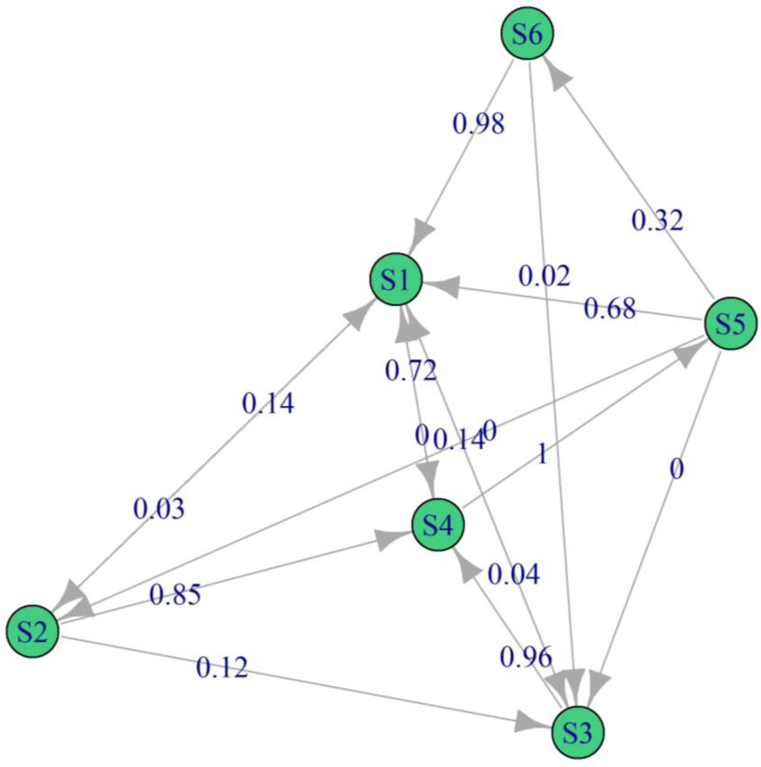
The relationships between the individual states are shown in Figure 1.

3.2. Studying Markov’s Property

In the first stage, the lack of memory characteristic of the process was assessed. The goodness of fit test ${\chi }^2$ was used for the study, defining at the level of significance $\alpha =0.05$ the zero hypothesis assuming that the chain studied meets the Markov property, and the alternative hypothesis that the Markov property is not met [11]. The test statistic ${\chi }^2=228.7$, while related to it p-value = 0.264, which means that there are no grounds to reject the zero hypothesis on the chain meeting the Markov property.

3.3. Fit of Distributions

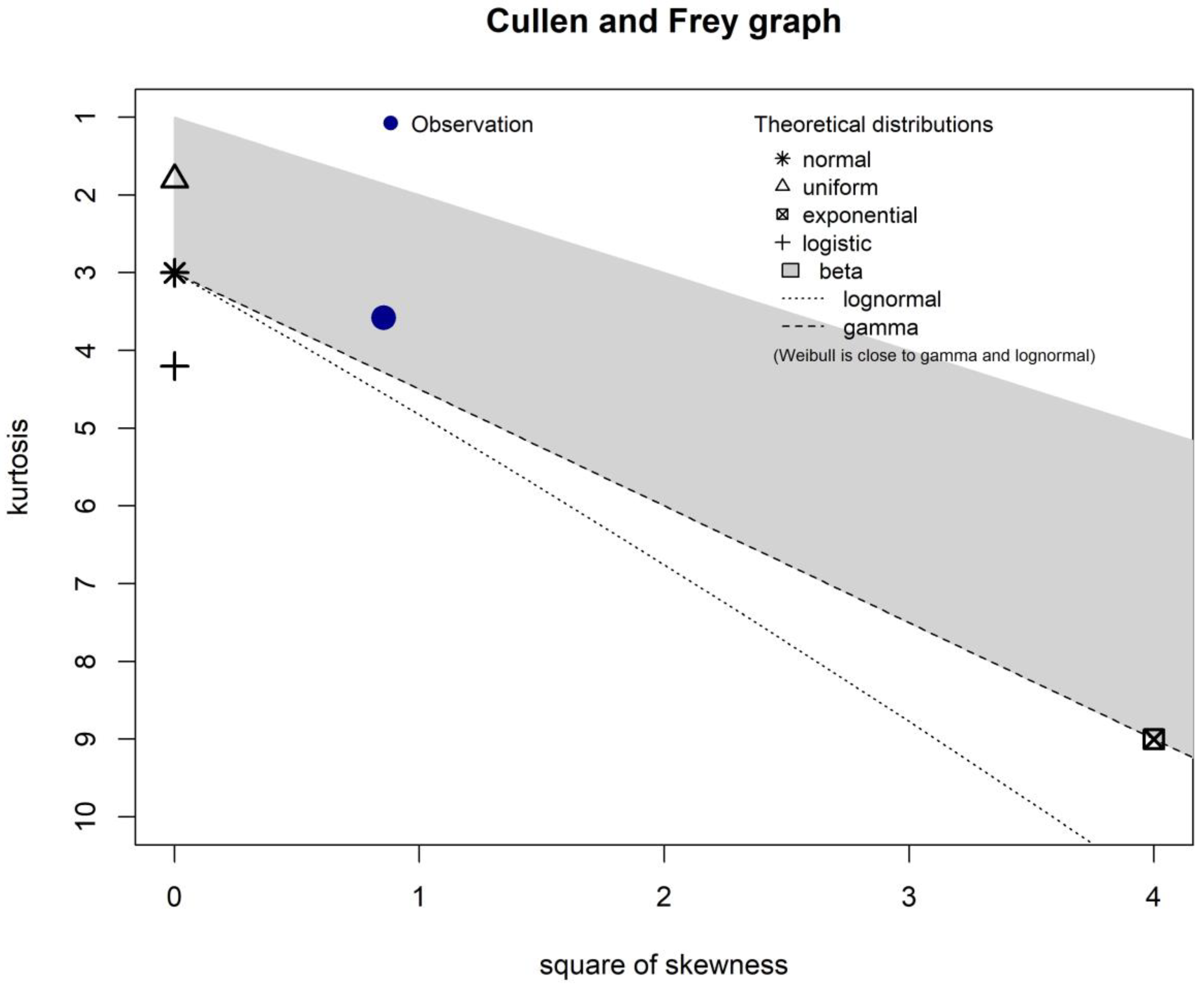
The next step was to assess the form of distributions of the individual states. Considerations in this respect were presented using the example of state S₆, and for the others the same was done. The goodness of fit to the selected theoretical distributions that were considered most likely was verified based on a Cullen and Frey graph, presented for state S₆ in Figure 2.

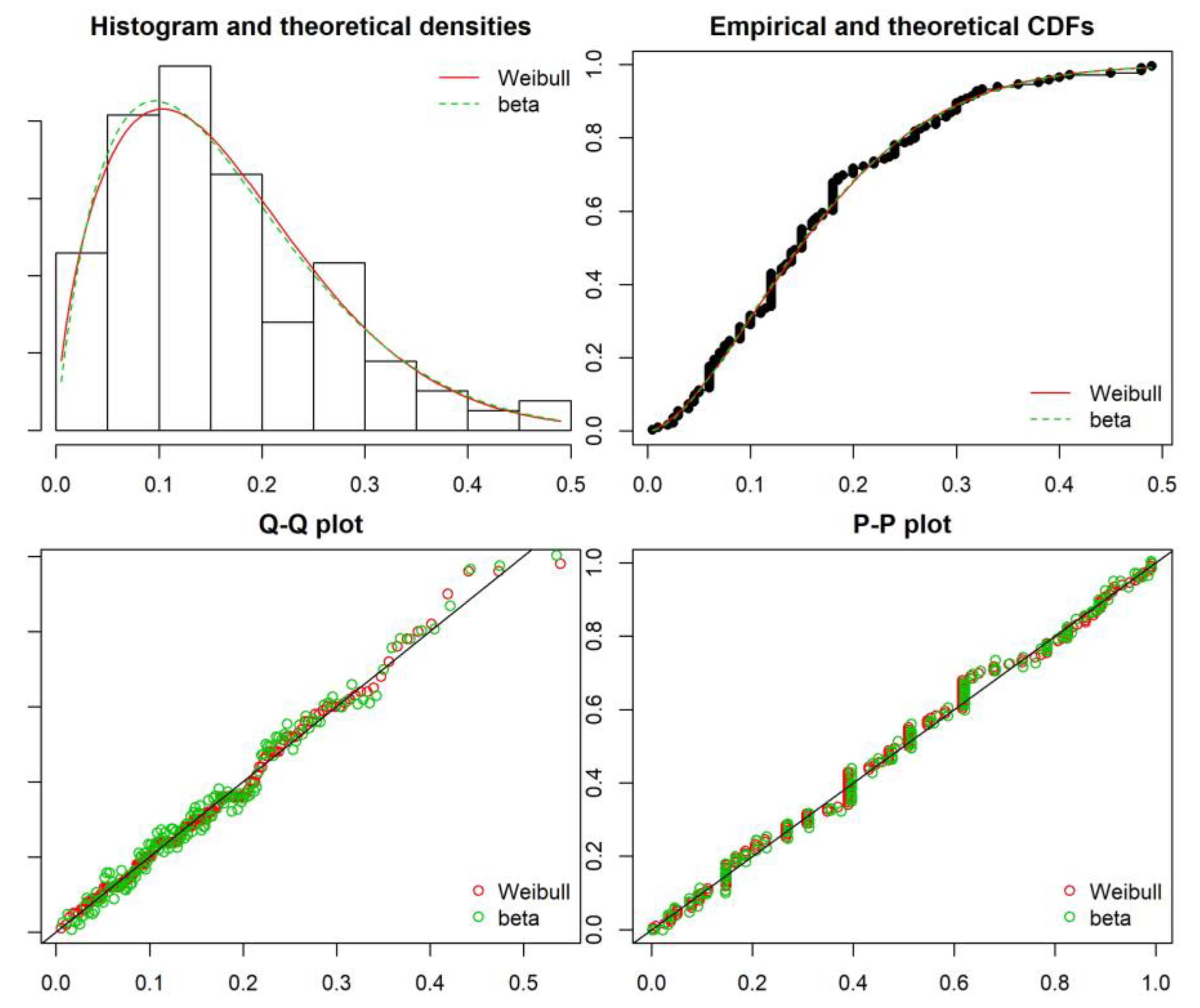
For further analysis, the Weibull and Beta distributions were selected, for which the estimated parameters are presented in

Table 2. Estimated model parameters according to Weibull and Beta distributions.

	Distribution Parameters		Kolmogorov–Smirnov Test Statistic	p-Value	Akaike Criterion
Weibull Distribution	Scale	Shape
Parameters	186.57	1.66	D = 0.07	0.385	1872.38
Std. Error	9.53	0.11
Beta distribution	shape 1	shape 2
Parameters	1.93	9.76	D = 0.06	0.56	−297.29
Std. Error	0.21	1.13

, while the goodness of fit of empirical data to the individual distributions is presented in Figure 3.

For each of them the $AIC$ (Akaike information criterion) was calculated according to the formula (16) and based on that, the one with the better fit was selected.

$$AIC=-2\ln L+2k,$$

(16)

where $k$—number of parameters in the model, $L$—credibility function.

The same calculations were made for the other states. The proposed distributions are presented in

Table 3. Goodness of fit results for states S₁–S₆.

State	Distribution	Test Statistic KS	p-Value
S1	non-parametric
S2	Beta	D = 0.07	0.793
S3	non-parametric
S4	Gamma	D = 0.03	0.726
S5	non-parametric
S6	Beta	D = 0.07	0.385

.

Not all the distributions could be fitted to the parametric ones. Moreover, none of the distributions belong to the family of exponential distributions, which is a condition for using the Markov process [25]. The form of distributions makes the parameters estimation possible based on the semi-Markov model only. In order to compare whether meeting the condition of the distribution form affects the obtained results, the subsequent part of the article compares the limit values of the probabilities of the object’s dwelling time according to two different models.

4. Case Study

4.1. Estimation of the Semi-Markov Model Parameters

First of all, based on the actual relationship between the states defined in Figure 1, the transition probability matrix was calculated. If $n_i$ denotes the number of instants of the system waiting in state $s_i$, while $n_{ij}$ denotes the number of state transitions from state $s_i$ to state $s_j$, then the transition estimator from state $s_i$ to state $s_j$ shall be determined from the formula:

$${\widehat{p}}_{ij}=\frac{n_{ij}}{n_i}.$$

(17)

The distribution of probability of changes of the distinguished operating states (in one step), assuming that each graph arch of the exploitation process representation (Equations (2) and (10)) corresponds to the value of probability $p_{ij}$, is presented in

Table 4. The $p_{ij}$ inter-states transition probability matrix.

${\mathit{p}}_{\mathit{i}\mathit{j}}$	S1	S2	S3	S4	S5	S6
S1	0	0.141	0.143	0.716	0	0
S2	0.029	0	0.117	0.854	0	0
S3	0.043	0	0	0.957	0	0
S4	0.003	0	0	0	0.997	0
S5	0.676	0.004	0.001	0	0	0.319
S6	0.982	0	0.018	0	0	0

.

For the process studied, some limits exist:

$$\underset{n\to \infty }{\lim }{p}_{ij}\left(n\right)={\pi }_j i, j=1,2,\dots ,6 i\ne j,$$

(18)

where $p_{ij}\left(n\right)$—probability of transition from state $S_i$ to state $S_j$ in $n$ steps.

Definition 2.

A probability distribution [25]:

$$\pi =\left[{\pi }_j: j\in S\right],$$

(19)

Satisfying a system of linear equations:

$${{\displaystyle \sum }}_{i\in S}{\pi }_i·p_{ij}={\pi }_j,j\in S,$$

(20)

and

$${{\displaystyle \sum }}_{iϵS}{\pi }_i=1,$$

(21)

is said to be a stationary probability distribution of the Markov chain witch transition matrix $P=\left[p_{ij}:i, j\in S\right]$. In matrix form, the Equation (20) takes the following form:

$${\mathsf{\Pi }}^{T}P={\mathsf{\Pi }}^T\leftrightarrow \left({\mathrm{P}}^T-I\right)·\mathsf{\Pi }=0,$$

(22)

Stationary probabilities ${\pi }_j$ were calculated in accordance with Equation (22). For the process studied, for the 6-state model, the determination of the stationary probabilities ${\pi }_j$ required solving the following matrix equation:

$${\left[\begin{array}{c}\begin{array}{c}{\pi }_1\\ {\pi }_2\\ {\pi }_3\end{array}\\ {\pi }_4\\ {\pi }_5\\ {\pi }_6\end{array}\right]}^T·\left[\begin{array}{cccccc}0& p_{12}& p_{13}& p_{14}& 0& 0\\ p_{21}& 0& p_{23}& p_{24}& 0& 0\\ p_{31}& 0& 0& p_{34}& 0& 0\\ p_{41}& 0& 0& 0& p_{45}& 0\\ p_{51}& p_{52}& p_{53}& 0& 0& p_{56}\\ p_{61}& 0& p_{63}& 0& 0& 0\end{array}\right]{=\left[\begin{array}{c}\begin{array}{c}{\pi }_1\\ {\pi }_2\\ {\pi }_3\end{array}\\ {\pi }_4\\ {\pi }_5\\ {\pi }_6\end{array}\right]}^T,$$

(23)

with the normalization condition:

$${\pi }_1+{\pi }_2+{\pi }_3+{\pi }_4+{\pi }_5+{\pi }_6=1,$$

(24)

which is equivalent to the following system of equations:

$$\{\begin{array}{l}{\pi }_2·p_{21}+{\pi }_3·p_{31}+{\pi }_4·p_{41}+{\pi }_5·p_{51}+{\pi }_6·p_{61}={\pi }_1\\ {\pi }_1·p_{12}+{\pi }_5·p_{52}={\pi }_2\\ {\pi }_1·p_{13}+{\pi }_2·p_{23}+{\pi }_5·p_{53}+{\pi }_6·p_{63}={\pi }_3\\ {\pi }_1·p_{14}+{\pi }_2·p_{24}+{\pi }_3·p_{34}={\pi }_4\\ {\pi }_4·p_{45}={\pi }_5\\ {\pi }_5·p_{56}={\pi }_6\\ {\pi }_1+{\pi }_2+{\pi }_3+{\pi }_4+{\pi }_5+{\pi }_6=1\end{array}.$$

(25)

After substituting the figures we get:

$$\{\begin{array}{l}{\pi }_2·0.029+{\pi }_3·0.043+{\pi }_4·0.003+{\pi }_5·0.676+{\pi }_6·0.982={\pi }_1\\ {\pi }_1·0.141+{\pi }_5·0.004={\pi }_2\\ {\pi }_1·0.143+{\pi }_2·0.117+{\pi }_5·0.001+{\pi }_6·0.018={\pi }_3\\ {\pi }_1·0.716+{\pi }_2·0.854+{\pi }_3·0.957={\pi }_4\\ {\pi }_4·0.997={\pi }_5\\ {\pi }_5·0.319={\pi }_6\\ {\pi }_1+{\pi }_2+{\pi }_3+{\pi }_4+{\pi }_5+{\pi }_6=1\end{array}.$$

(26)

The solution are the stationary probabilities presented in

Table 5. Stationary probabilities of the Markov chain.

	S1	S2	S3	S4	S5	S6
$p_{ij}$	0.276	0.04	0.046	0.276	0.275	0.088

.

The analysis of the stationary distribution showed (Table 5) that the limit highest transitions probabilities concern states (S₁, S₄, S₅) related to standard activities resulting from the production process technology (all over 27%). Indications of undesirable conditions such as failure (S₂) or downtime (S₃, S₆) range from 4% to 8%, which is a good result.

The calculated limit probabilities relate to the frequency of observations in the sample and do not take into account the duration of individual states, therefore, the limit distribution of the semi-Markov process represents more significant diagnostics. It can be determined using the stationary distribution of the Markov chain and the expected duration of the process states [24,25]. Then the limit probabilities of semi-Markov process are expressed by the formula:

$$P_j=\underset{t\to \infty }{\lim }P\left(t\right)=\frac{{\pi }_{j}E\left({\mathrm{T}}_j\right)}{{{\displaystyle \sum }}_{j\in S}{\pi }_{j}E\left({\mathrm{T}}_j\right)}.$$

(27)

The solution requires to calculate the following forms from the sample of average conditional durations of the process states:

$$\mathrm{T}=\left[{\overline{T}}_{ij}\right],i,j =1, 2, \dots , 6.$$

(28)

that are presented in

Table 6. Average conditional durations of the semi-Markov process states.

$\overline{T}{ }_{\mathit{i}\mathit{j}} \left[\mathit{m}\mathit{i}\mathit{n}\mathit{u}\mathit{t}\mathit{e}\mathit{s}\right]$	S1	S2	S3	S4	S5	S6
S1		795.48	637.63	1082.14
S2	4800		256.67	277.27
S3	4020			508.6
S4	21.5				248.62
S5	42.33	40	15			40.36
S6	156.3		226.25

.

Based on the transitions probabilities matrix $P=\left[p_{ij}\right]$ (Table 5) and the matrix of average conditional durations of the states of the process $\mathrm{T}=\left[T{}_{ij}\right]$ of random variables ${\overline{T}}_{ij}$ (Table 6), dependencies describing average unconditional durations of the process states were determined ${\overline{T}}_j$ according to the formula:

$${\overline{T}}_j={{\displaystyle \sum }}_{i=1}^6{p}_{ij} {\overline{T}}_{ij}.$$

(29)

For this purpose, the following equation system was solved:

$$\{\begin{array}{l}{\overline{T}}_1=p_{12}·T_{12}+p_{13}·T_{13}+p_{14}·T_{14}\\ {\overline{T}}_2=p_{21}·T_{21}+p_{23}·T_{23}+p_{24}·T_{24}\\ {\overline{T}}_3=p_{31}·T_{31}+p_{34}·T_{34}\\ {\overline{T}}_4=p_{41}·T_{41}+p_{45}·T_{45}\\ {\overline{T}}_5=p_{51}·T_{51}+p_{52}·T_{52}+p_{53}·T_{53}+p_{56}·T_{56}\\ {\overline{T}}_6=p_{61}·T_{61}+p_{63}·T_{63}\end{array}.$$

(30)

The obtained expected values of unconditional dwelling ${\overline{T}}_i$ times of the process X(t) in the individual operational states are presented in

Table 7. Unconditional times ${\overline{T}}_i \left[\mathrm{minutes}\right]$ for the 6-state model.

	$\overline{T}{ }_1$	$\overline{T}{ }_2$	$\overline{T}{ }_3$	$\overline{T}{ }_4$	$\overline{T}{ }_5$	$\overline{T}{ }_6$
${\overline{T}}_{\mathrm{i}}\left[minutes\right]$	978.16	406.02	659.59	247.96	41.67	157.56

.

The calculated random variables ${\mathrm{T}}_i$ have finite, positive expected values. This allows to calculate, based on theorem (27), the limit probabilities $P_j$ which are presented in

Table 8. Values of limit probabilities $P_j$ of the 6-state model.

$P_1$	0.6579	$P_1 [\%]$	65.79
$P_2$	0.0396	$P_2$ [%]	3.96
$P_3$	0.0740	$P_3 [\%]$	7.4
$P_4$	0.1667	$P_4[\%]$	16.67
$P_5$	0.0279	$P_5$ [%]	2.79
$P_6$	0.0337	$P_6$ [%]	3.37

.

Thus determined probabilities $P_j$ are limit probabilities determining that the system will remain, for a longer period ($t\to \infty$), in the given operational state. This prognosis is more satisfactory than for the frequency of the states occurring. The highest values are achieved by state S₁, i.e., operation (over 65%) and less than 17% by state S₄, which stems from the necessity to perform maintenance activities. The remaining limit values are satisfactorily small, which shows the correct operation of the machines.

The technical readiness factor was also determined in the form of the sum of appropriate probabilities of reliability states [34]. For the system under analysis, $S_1$, $S_4$, $S_5$ were considered as fitness states, while the states $S_2$ $S_3$ and $S_6$ as unfitness states. Then, the readiness of the 6-element semi-Markov model can be calculated as the sum of limit probabilities of the respective states:

$$K={{\displaystyle \sum }}_j{P}_j=P_1+P_4+P_5,$$

(31)

This gives $K=0.85$, which means that the machine is in the readiness state for over 85% of the time, which is a very good result.

4.2. Calculations According to the Markov Model

Markov processes concern exponential distributions, the most popular ones in reliability theory [11,35]. They are described by two parameters, which fully define them. The first of these is the already calculated probability matrix of interstate transitions $p_{ij}$ (Table 4).

The second, important parameter is the function describing the transitions of objects between states, called the process transition intensity ${\lambda }_{ij}\left(t\right)$, which characterizes the rate of changes in the probability of transition $p_{ij}\left(t\right)$ [36].

$${\lambda }_{ij}\left(t\right)=\underset{\Delta t\to 0}{\lim }\frac{1}{\Delta t}{p}_{ij}\left(t,t+\Delta t\right)\mathrm{for}i,j=0,1,2,\dots i\ne j,$$

(32)

For homogeneous Markov processes, the transition intensity is constant and equal to the inverse of the expected duration $t_{ij}$ of the state $S_i$ before $S_j$ [37]:

$${\lambda }_{ij}\left(t\right)=\frac{1}{\mathrm{E}\left(t_{ij}\right)},$$

(33)

where:

• ${\lambda }_{ij}\left(t\right)$—intensity of transitions from the state $i$ to state $j$,
• $E(t_{ij})$—expected duration value $t_{ij}$.

The intensities ${\lambda }_{ii}\le 0$ for $i=j$ are defined as a complement to the sum of transition intensity from state S_i for $i \ne j$ to 0:

$${\lambda }_{ii}+{\Sigma }_j {\lambda }_{ii}=0$$

(34)

thus:

$${\lambda }_{ii}=-{\Sigma }_j {\lambda }_{ii}.$$

(35)

The modules $\left|{\lambda }_{ii}\right|=-{\lambda }_{ii}$ are called the exit intensities from the state $S_i$.

Calculated according to the above formulas (33)–(35), the element ${\lambda }_{ij}$ of the matrix $\Lambda$ of transition intensity is shown in

Table 9. The transition intensity matrix of the process studied.

$\mathit{\lambda }{ }_{\mathit{i}\mathit{j}} \left[1/\mathit{m}\mathit{i}\mathit{n}\mathit{u}\mathit{t}\mathit{e}\mathit{s}\right]$	S1	S2	S3	S4	S5	S6
S1	−0.0037	0.0013	0.0016	0.0009	0	0
S2	0.0002	−0.0077	0.0039	0.0036	0	0
S3	0.0002	0	−0.0022	0.0020	0	0
S4	0.0465	0	0	−0.0505	0.0040	0
S5	0.0236	0.0250	0.0667	0	−0.1401	0.0248
S6	0.0064	0	0.0044	0	0	−0.0108

.

Then, using the relationship (36), ergodic probabilities $p_j$ were calculated for the Markov model in continuous time.

$${{\displaystyle \prod }}^T\ast \Lambda =0,$$

(36)

where:

• ${{\displaystyle \prod }}^T={\left[p_j\right]}^T=\left[p_1;;p_{ns}\right]$—transposed vector of limit probabilities $p_j$,
• $\left|\mathsf{\Lambda }\right|$—transition intensity matrix:
• ${{\displaystyle \sum }}_j{p}_j=1$—the normalization condition.

This way, for the process studied, we obtain the following matrix Equation (37):

$${\left[\begin{array}{c}{p}_1\\ p_2\\ p_3\\ p_4\\ p_5\\ p_6\end{array}\right]}^T·\left[\begin{array}{cccccc}-{\lambda }_{11}& {\lambda }_{12}& {\lambda }_{13}& {\lambda }_{14}& 0& 0\\ {\lambda }_{21}& -{\lambda }_{22}& {\lambda }_{23}& {\lambda }_{24}& 0& 0\\ {\lambda }_{31}& 0& -{\lambda }_{33}& {\lambda }_{34}& 0& 0\\ {\lambda }_{41}& 0& 0& -{\lambda }_{44}& p_{45}& 0\\ {\lambda }_{51}& {\lambda }_{52}& {\lambda }_{53}& 0& -{\lambda }_{55}& {\lambda }_{56}\\ {\lambda }_{61}& 0& {\lambda }_{63}& 0& 0& -{\lambda }_{66}\end{array}\right]=\left[\begin{array}{c}0\\ 0\\ 0\\ 0\\ 0\\ 0\end{array}\right],$$

(37)

Taking into account the normalization condition: ${{\displaystyle \sum }}_{j=1}^6{p}_j=1$, we get the limit probabilities $p_j$ of the system’s dwelling time in the states S₁–S₆, which are shown in

Table 10. Limit probabilities $p_j$ in the continuous physical time for the Markov process.

	S1	S2	S3	S4	S5	S6
$p_j$	0.4228	0.0742	0.4695	0.0306	0.0009	0.0020
$p_{j\%}$	42.28	7.42	46.95	3.06	0.09	0.20

.

The results obtained deviate from the values determined for the semi-Markov process, disturbingly revealing that the system studied tends primarily to remain in the downtime state (S₃). The state in which the production takes place (S₁) comes only second and takes the value lower by over 35% in relation to calculations made according to the semi-Markov process. A comparison of the other results is presented in

Table 11. Comparison of results for the Markov and semi-Markov models.

	S1	S2	S3	S4	S5	S6
$p_j$ semi-Markov model	0.6589	0.0396	0.074	0.1667	0.0279	0.0337
$p_j$ Markov model	0.4228	0.0742	0.4695	0.0306	0.0009	0.0020
difference in %	−35.74	87.41	534.50	−81.65	−96.87	−94.05

. The highest difference concerns state S₃, and is over 534%.

The technical readiness coefficient was also calculated based on the (31), which for the Markov process amounts to 45% ($K=0.45$)—almost half the size of what was determined according to the semi-Markov process.

5. Conclusions

The study achieved two important goals. The first of them was a presentation of the method of evaluating the readiness of a selected element of a machine tools in the production system. The analysis according to the Markov chain allowed to determine the probabilities of interstate transitions, which reflect the frequency of the occurrence of individual states. The highest values were achieved for relations S₆–S₄, S₃–S₄, S₄–S₅. They suggest a high incidence of unsuitability states—S₃ and S₆—and the need to determine their causes and reduce their occurrence.

The limit values of transition probability were also calculated. The analysis of stationary distribution showed that the greatest indications concern states related to activities resulting from production process technology (S₁, S₄, S₅), which is a good result.

However, a complete evaluation is only ensured by an analysis according to the semi-Markov process, taking into account the average dwell times of an object in the individual operating states. The calculated probability limits, examining the behavior of the object for $t\to \infty$, were the highest for state S₁—operation (over 65%) and state S₄—service (almost 17%). The remaining limit values were found to be satisfactorily low, which means that the operation of the machine should be considered as proper. The calculated technical readiness rate of 85% should also be viewed as positive.

Such an analysis not only provides information on the assessment of the current and expected functioning of the machine, but also reveals areas where modifications can be made in order to increase the level of availability and, as a result, ensure more efficient execution of production orders.

Another goal was to compare the results according to the assumptions made, concerning the forms of distribution of the examined variables. In the literature this analysis is often omitted and it is assumed that the examined variable has an exponential distribution. This allows to use Markov’s processes, whose parameter estimation is simpler and is described in more detail in publications. Such an assumption—as the study has shown—may lead to different results and effectively to form an incorrect assessment of the process/system studied. The intention of the authors was to indicate that omitting an important stage of statistical analysis of the collected data and assuming a priori the form of distributions does not guarantee the correctness of the obtained analyses.

In the presented study, the differences in the values of the calculated limit probabilities are large, reaching even over 530%. The overall evaluation of system readiness indicates a value lower by 46% in the case of the Markov process analysis.

However, the problem is not only the value of the calculated probabilities, but also the main aim of the system. According to the semi-Markov process, the system tends primarily to occupy state $S_1$ (operation) which is a satisfactory result, emphasizing the proper implementation of tasks. The results according to the Markov process show that the system tends to occupy mainly state $S_3$—downtime, which indicates mismanagement and system inactivity.

The goals set by the authors have been achieved, but it should be stressed out that the results obtained concern only one selected machine. As part of further research, it is worth considering a comprehensive analysis of the entire production system using the method indicated in the article. It will provide complete information on its readiness, determine the level of impact of individual elements (machines), and identify areas for improvement.

References

- Kozłowski, E.; Mazurkiewicz, D.; Żabiński, T.; Prucnal, S.; Sęp, J. Assessment model of cutting tool condition for real-time supervision system. Eksploat. Niezawodn. Maint. Reliab. 2019, 21, 679–685. [Google Scholar] [CrossRef]
- Kosicka, E.; Kozłowski, E.; Mazurkiewicz, D. The use of stationary tests for analysis of monitored residual processes. Eksploat. Niezawodn. Maint. Reliab. 2015, 17, 604–609. [Google Scholar] [CrossRef]
- Jasiulewicz-Kaczmarek, M.; Żywica, P. The concept of maintenance sustainability performance assessment by integrating balanced scorecard with non-additive fuzzy integral. Eksploat. Niezawodn. Maint. Reliab. 2018, 20, 650–661. [Google Scholar] [CrossRef]
- Antosz, K. Maintenance—Identification and analysis of the competency gap. Eksploat. Niezawodn. Maint. Reliab. 2018, 20, 484–494. [Google Scholar] [CrossRef]
- Kishawy, H.A.; Hegab, E.; Umer, U.; Mohany, A. Application of acoustic emissions in machining processes: Analysis and critical review. Int. J. Adv. Manuf. Technol. 2018, 98, 1391–1407. [Google Scholar] [CrossRef]
- Rymarczyk, T.; Kozłowski, E.; Kłosowski, G.; Niderla, K. Logistic Regression for Machine Learning in Process Tomography. Sensors 2019, 19, 3400. [Google Scholar] [CrossRef] [Green Version]
- Fisz, M. Rachunek Prawdopodobieństwa i Statystyka Matematyczna; PWN: Warszawa, Poland, 1967. [Google Scholar]
- Zhang, Y.; Zhang, Q.; Yu, R. Markov property of Markov chains and its test. In Proceedings of the International Conference on Machine Learning and Cybernetics, Qingdao, China, 11–14 July 2010; pp. 1864–1867. [Google Scholar] [CrossRef]
- Chen, B.; Hong, Y. Testing for the Markov property in time series. Econ. Theory 2012, 28, 130–178. [Google Scholar] [CrossRef]
- Shi, S.; Lin, N.; Zhang, Y.; Cheng, J.; Huang, C.; Liu, L.; Lu, B. Research on Markov property analysis of driving cycles and its application. Transp. Res. Part D Transp. Environ. 2016, 47, 171–181. [Google Scholar] [CrossRef]
- Kozłowski, E.; Borucka, A.; Świderski, A. Application of the logistic regression for determining transition probability matrix of operating states in the transport systems. Eksploat. Niezawodn. Maint. Reliab. 2020, 22, 192–200. [Google Scholar] [CrossRef]
- Yang, H.; Nair, V.N.; Chen, J.; Sudjianto, A. Assessing Markov property in multistatetransition models with applications to credit risk modeling. Appl. Stoch. Models Business Ind. 2019, 35, 552–570. [Google Scholar] [CrossRef]
- Komorowski, M.; Raffa, J. Markov Models and Cost Effectiveness Analysis: Applications in Medical Research. In Secondary Analysis of Electronic Health Records; Springer: Cham, Switzerland, 2016; pp. 351–367. [Google Scholar]
- Gercbach, I.B.; Kordonski, C.B. Modele Niezawodnościowe Obiektów Technicznych; WNT: Warszawa, Poland, 1968. [Google Scholar]
- Gichman, I.I.; Skorochod, A.W. Wstęp Do Teorii Procesów Stochastycznych; PWN: Warszawa, Poland, 1968. [Google Scholar]
- Li, Y.; Dong, Y.; Zhang, H.; Zhao, H.; Shi, H.; Zhao, X. Spectrum Usage Prediction Based on High-order Markov Model for Cognitive Radio Networks. In Proceedings of the 10th IEEE International Conference on Computer and Information Technology, Bradford, UK, 29 June–1 July 2010; pp. 2784–2788. [Google Scholar] [CrossRef]
- Perman, M.; Senegacnik, A.; Tuma, M. Semi-Markov models with an application to power-plant reliability analysis. IEEE Transac. Reliab. 1997, 46, 526–532. [Google Scholar] [CrossRef]
- Lana, X.; Burgueño, A. Daily dry–wet behaviour in Catalonia (NE Spain) from the viewpoint of Markov chains. Int. J. Climatol. 1998, 18, 793–815. [Google Scholar] [CrossRef]
- Pang, W.; Forster, J.J.; Troutt, M.D. Estimation of Wind Speed Distribution Using Markov Chain Monte Carlo Techniques. J. Appl. Meteorol. 2010, 40, 1476–1484. [Google Scholar] [CrossRef]
- Love, C.E.; Zhang, Z.G.; Zitron, M.A.; Guo, R. A discrete semi-Markov decision model to determine the optimal repair/replacement policy under general repairs. Eur. J. Oper. Res. 2010, 125, 398–409. [Google Scholar] [CrossRef]
- Doob, J.L. Stochastic Processes; John Wiley & Sons/Chapman & Hall: New York, NY, USA, 1953. [Google Scholar]
- Iosifescu, M. Finite Markov Processes and Their Applications; John Wiley & Sons: Chichester, UK, 1980. [Google Scholar]
- Howard, R.A. Dynamic Probabilistic System, Volume II: Semi-Markow and Decision Processes; Wiley: New York, NY, USA, 1971. [Google Scholar]
- Jaźwiński, J.; Grabski, F. Niektóre Problemy Modelowania Systemów Transportowych; Biblioteka Problemów Eksploatacji: Warszawa, Poland, 2003. [Google Scholar]
- Grabski, F. Semi-Markow Processes: Applications in System Reliability and Maintenance; Elsevier: Gdynia, Poland, 2014. [Google Scholar]
- Geng, J.; Xu, S.; Niu, J.; Wei, K. Research on technical condition evaluation of equipments based on matter element theory and hidden Markov model. In Proceedings of the 4th Annual International Workshop on Materials Science and Engineering (IWMSE2018), Xi’an, China, 18–20 May 2018; Volume 381, p. 012134. [Google Scholar] [CrossRef] [Green Version]
- Yuriy, E.; Obzherin, M.; Siodorov, S. Application of hidden Markov models for analyzing the dynamics of technical systems. AIP Conf. Proc. 2019, 2188, 050019. [Google Scholar] [CrossRef]
- Iscioglu, F.; Kocak, A. Dynamic reliability analysis of a multi-state manufacturing system. Eksploat. Niezawodn. Maint. Reliab. 2019, 21, 451–459. [Google Scholar] [CrossRef]
- Liu, C.; Duan, H.; Chen, P.; Duan, L. Improve Production Efficiency and Predict Machine Tool Status using Markov Chain and Hidden Markov Model. In Proceedings of the 8th International Conference of Computer Science and Information Technology (CIST), Amman, Jordan, 26–28 May 2018; pp. 276–281. [Google Scholar] [CrossRef]
- Gola, A. Reliability analysis of reconfigurable manufacturing system structures using computer simulation methods. Eksploat. Niezawodn. Maint. Reliab. 2019, 21, 90–102. [Google Scholar] [CrossRef]
- Wang, C.H.; Sheu, S.H. Determining the optimal production-maintenance policy with inspection errors: Using a Markov chain. Comput. Oper. Res. 2003, 30, 1–17. [Google Scholar] [CrossRef]
- Dung, K.; Lei, J.; Chan, F.; Hui, J.; Zhang, F.; Wang, Y. Hidden Markov model-based autonomous manufacturing task orchestration in smart shop floors. Robot. Comput. Integr. Manuf. 2020, 61, 101845. [Google Scholar] [CrossRef]
- Xiang, L.; Guan, J.; Wu, S. Measuring the impact of final demand on global production system based on Markov process. Phys. A Stat. Mech. Appl. 2018, 502, 148–163. [Google Scholar] [CrossRef]
- Żurek, J.; Tomaszewska, J. Analiza system eksploatacji z punktu widzenia gotowości. Prace Nauk. Politech. Warsz. 2016, 114, 471–477. [Google Scholar]
- Pavlov, N.; Golev, A.; Rahney, A.; Kyurkchiev, N. A Note on the Generalized Inverted Exponential Software Reliability Model. Int. J. Adv. Res. Comput. Commun. Eng. 2018, 7, 484–487. [Google Scholar]
- Borucka, A.; Niewczas, A.; Hasilova, K. Forecasting the readiness of special vehicles using the semi-Markov model. Eksploat. Niezawodn. Maint. Reliab. 2019, 21, 662–669. [Google Scholar] [CrossRef]
- Filipowicz, B. Modele Stochastyczne w Badaniach opeRacyjnych, aNaliza i Synteza Systemów Obsługi i Sieci Kolejkowych; Wydawnictwa Naukowo-Techniczne: Warszawa, Poland, 1996. [Google Scholar]
Figure 1.
Diagram of the inter-state transitions of the process studied.
Figure 2.
Cullen and Frey graph for the state S6.
Figure 3.
The assessment of goodness of fit of the empirical data of state to the Weibull and Beta distributions.