A Hybrid Double Forecasting System of Short Term Power Load Based on Swarm Intelligence and Nonlinear Integration Mechanism

Abstract

Accurate and reliable power load forecasting not only takes an important place in management and steady running of smart grid, but also has environmental benefits and economic dividends. Accurate load point forecasting can provide a guarantee for the daily operation of the power grid, and effective interval forecasting can further quantify the uncertainty of power load on this basis to provide dependable and precise load information. However, most of the previous work focuses on the deterministic point prediction of power load and rarely considers the interval prediction of power load, which makes the prediction of power load not comprehensive. In this study, a new double hybrid load forecasting system including point forecasting module and interval forecasting module is developed, which can make up for the shortcomings of incomplete analysis for the existing research. The point forecasting module adopts a nonlinear integration mechanism based on Back Propagation (BP) network optimized by Multi-objective Evolutionary Algorithm based on Decomposition (MOEA/D) to improve the accuracy of point prediction. A fuzzy clustering interval prediction method based on different data feature classification is successfully proposed which provides an effective tool for load uncertainty analysis. The experiment results show that the system not only has a good effect in accurately predicting power load, but also can analyze the uncertainty of the power load, which can be used as an effective technology of power system planning.

1. Introduction

Power load forecasting is the foundation and key task of management and control of power system [1]. It is often applied in energy supervise, unit commitment and load control [2]. High precision load prediction ensures the secure and steady operation of power system [3]. Therefore, it is essential to enhance the deliverability and prediction precision of smart grid [4]. However, due to many indeterminate reasons such as climate variation, economy growth, public activities and national decisions, the accuracy of power load forecast often fails to achieve the expected results [5]. In view of this, all countries in the world are looking for effective load forecast methods to enhance the accuracy of load forecasting [6].

In addition, the combination of ultra-short term load forecast (USTLF), short term load forecast (STLF), medium and long term load forecast (LTLF) is significant to the safe and economic operation of power system [7]. USTLF and STLF are the necessary basis of power grid dispatching, and reducing the error of STLF is an effective method to strengthen the supervising level of power system [8]. Accurate prediction of power load can save a lot of time to manage the power grid and avoid major changes [9]. Therefore, it is essential to establish a load prediction model with high forecast ability. For the sake of achieve precise and steady STLF, researchers have adopted a lot of methods, including (a) statistical method, (b) artificial intelligence method and (c) hybrid method [10].

In the early stage of power load forecasting, traditional statistical methods are often applied, including some conventional forecasting methods, such as regression method [11], exponential smoothing [12], Autoregressive Moving Average Model (ARMA) [13], Autoregressive Integrated Moving Average (ARIMA) [14,15], seasonal ARIMA [16], grey forecasting model (GM) [17], etc. These models could obtain power load prediction, but due to their own limitations, they cannot achieve the expected forecasting accuracy. In order to overcome these limitations, more and more effective load forecasting approaches have been put forward. In recent years, the prediction model based on artificial intelligence is gradually springing up in electric load prediction [18]. At the moment, the algorithms of artificial intelligence mainly include artificial neural network (ANN) [19,20], support vector machine (SVM) [21], multi-layer perceptron (MLP) and radial basis function (RBF). Although better than the traditional methods, they still unable to fit the current complicated and variable power load characteristics well to achieve satisfactory accuracy due to the defects of a single prediction method [22]. For example, the artificial neural network is easy to fall into local optimization, over fitting and low convergence rate [23]. This has led to the largely establishment of integrating and hybrid models, which are composed of several single models and can achieve better prediction performance [24].

Xiaobo Zhang et al. [25] successfully proposed a new power load prediction model, CS-SSA-SVM, which integrated singular spectrum analysis (SSA), support vector machine (SVM) and cuckoo search (CS) algorithm. This model can significantly enhance the effectiveness of power load forecast. Dong, Y. et al. [26] developed a short-term load prediction model using a unit for feature learning named Pyramid System and recurrent neural networks, and it can greatly increase the stabilization and safety of the smart grid. Wang, R. et al. [27] proposed a new power load forecasting system by combining data preprocessing, hybrid optimized algorithm and certain individual conventional prediction methods, which conquers the shortcomings of individual conventional prediction model and obtains a single model optimization with higher prediction accuracy than traditional forecasting model.

Another problem of power load forecasting is that the research direction is relatively single. Specifically, most of the previous analysis only focuses on the point prediction of load, and rarely considers the load interval prediction together to prediction modeling and analysis. This is not enough to meet the needs of engineering applications, or to ensure the reliability of the power system. Probability interval prediction can display more messages, and its results can help managers to implement appropriate policies. However, the research on interval modeling and prediction is still lacking. At present, the main research direction of uncertainty quantification is mainly statistical methods, including quantile regression [28], bootstrap method [29], kernel density estimation [30], etc. in addition, there are interval prediction methods based on artificial neural network, including lower upper bound estimation method (LUBE) and so on [31].

Table 1. Summary of point prediction and interval prediction models.

Method	Advantage	Disadvantage
Point Forecasting
Statistical models (AR, ARIMA, fractional-ARIMA.)	Consider information from historical data High calculation efficiency Few adjustable model parameters Can mine the linear law of data effectively	Cannot mine the nonlinear law of data Stable data only Assuming the interference sequence is white noise is necessary
Artificial neural network	Can fit the non-linear patterns of data, and has good generalization ability and self-learning ability	The calculation process is complex High requirements on the number of training samples Fall into local optimum easily
Hybrid model	Integrate the advantages of each single model Improvement of prediction accuracy	Improved spaces in each part of the model still exist Non-linear patterns of data cannot be further mined by linear combination
Interval Forecasting
Quantile regression	Be able to deal with heterogeneity High tolerance for outliers Consider the whole distribution Ability to capture tail features of distribution	High training data set requirements Large amount of calculation Results are easily discarded
Bootstrap methods	Avoid possible discarding in quantile regression Very effective when handling small samples	Poor performance in handling large samples Large amount of computation
Kernel density estimation	Fast construction prediction interval	Strict distribution assumption
LUBE	Avoid the data distribution hypothesis High calculation efficiency Model coefficient is easy to adjust	The objective function is complex Traditional mathematical methods cannot optimize the objective function

summarizes the existing point prediction and interval prediction methods and models, and evaluates the advantages and disadvantages of these methods.

For point forecasting, from the traditional statistical model to the artificial neural network model, and even for the recently developed hybrid model, the prediction accuracy has been continuously improved, but the models still have a lot of space for improvement. According to the nonlinear characteristics of load, this paper proposes a method of nonlinear combination of single prediction model, and uses swarm intelligence optimization algorithm to optimize the model parameters to further improving the prediction effect. For interval forecasting, no matter quantile regression method [32], bootstrap method [33], kernel density estimation method [34] or LUBE method, these methods have their own advantages and disadvantages that are difficult to overcome. In conclusion, the interval prediction method is not uniform and further research and investigation are needed according to the existing knowledge to obtain more effective results [35]. Therefore, based on the hypothesis of distribution, this study develops a new architecture of interval prediction, which is better than most single model interval prediction architectures.

According to the review of the above literature and methods, the major contribution of this article is to design a hybrid double prediction system, including two parts: point forecasting and interval forecasting, which make up for the shortcomings of the existing research. Specifically, the double prediction system includes the preprocessing module based on Improved Complete Ensemble Empirical Mode Decomposition (ICEEMDAN), the prediction module based on nonlinear combination model, the interval prediction module and the evaluation module. As a new signal processing technology, ICEEMDAN decomposes and reconstructs the power load sequence to get a clear time sequence. The nonlinear combination model is an effective prediction model proposed in this study. Among it, Extreme Learning Machine (ELM) [36], RBF, Elman Neural Network (ENN) and ARIMA [37] are selected as the basic models of the combination model, and the prediction results of these four models are nonlinear aggregated by BP [38] neural network. BP network is very sensitive to the selection of parameters, which directly affects the validity of point prediction and interval prediction. Therefore, in order to find the optimal parameters in BP model, Multi-objective Evolutionary Algorithm based on Decomposition (MOEA/D) is developed effectively. Finally, an interval prediction method based on fuzzy clustering is established, which does not need the hypothesis of distribution and model. Therefore, the interval structure has a strong anti-interference ability to the abnormal values in the interval data. In addition, to testify the ability of the designed prediction architecture, we select 9 indicators to verify the accuracy of the prediction, and implement a series of discussion to judge the effectiveness of the prediction system.

The leading innovations of the forecasting system are summed up bellow:

(1) A new double forecasting system for power load is established in this paper, which is successfully combined of point forecasting module and interval forecasting module. The purpose of the system is to improve the accuracy of load point prediction, and effectively analyze the uncertainty of power load data.

(2) A nonlinear combination method based on the BP algorithm optimized by MOEA/D is proposed to better improve the forecasting performance of the system. To obtain the optimal combination pattern of each model, the nonlinear aggregation mechanism based on BP is adopted to combine the models and eliminate the inherent defects of individual model and linear combination. In particular, MOEA/D algorithm is used to search the best parameters of BP, which further improves the prediction accuracy.

(3) An interval prediction method based on fuzzy clustering is established, which provides an effective tool for load uncertainty analysis. The interval forecasting method determines the upper and lower bounds of the power load prediction value to quantify the uncertainty information of the load, and provide more comprehensive reference information for the operation risk decision makers of power system.

The rest of this paper is: Section 2 shows the methods applied in the proposed double forecasting architecture. In Section 3, the double forecasting system is established. Section 4 introduces the experimental data and displays the experimental results. Section 5 provides further discussion. Finally, the conclusion is given in Section 6.

2. Knowledge and Tools of Model Preparation

In constructing our model, several methods are chosen as the best choice, and they are combined to improve the ability of the model. Here we introduce three main methods named improved complete ensemble empirical mode decomposition (ICEEMDAN), multi-objective evolutionary algorithm based on decomposition (MOEA/D) and Fuzzy C-Means (FCM) clustering algorithm in detail.

The first is improved complete ensemble empirical mode decomposition (ICEEMDAN).

Being an effective data processing method, ICEEMDAN is proposed by Colominas, Schlotthauer and Torres [39] in 2014. It disintegrates the actual series into some intrinsic mode functions (IMF) and a residual from high frequency to low frequency. CEEMDAN has been proposed to restore the integrity property of EMD.

Nevertheless, CEEMDAN is still worthy of improvement in mode and signal decomposition. In ICEEMDAN, ${\mathit{F}}_k(\cdot )$ represents the operator figures out the k-th mode achieved by EMD, ${\mathit{\omega }}^{(i)}$ is the formation of Gaussian white noise that has zero mean and unit variance, and ${\mathit{x}}^{(i)}=\mathit{x}+{\mathit{\omega }}^{(i)}$. $\mathit{M}(\cdot )$ is the operator and it can produce the local average of the signal. Then ${\mathit{E}}_1(\mathit{z})=\mathit{z}-\mathit{M}(\mathit{z})$ can be obtained. The general steps of ICEEMDAN are as follows:

Step 1. The first residue is obtained by calculating the local averages of I formations ${\mathit{x}}^{(i)}=\mathit{x}+{\beta }_0{\mathit{E}}_1({\mathit{\omega }}^{(i)})$ (i = 1, …, I) using EMD:

$${\mathit{r}}_1=\langle \mathit{M}({\mathit{x}}^{(i)})\rangle ,(i=1,\dots ,I)$$

(1)

In the formula, ${\beta }_0={\epsilon }_0\cdot \mathit{S}(\mathit{x})/\mathit{S}({\mathit{E}}_1({\mathit{\omega }}^{(i)}))$, and ${\epsilon }_0$ is the reciprocal of the expected signal-to-noise ratio between the first additional noise and the analytical signal. $\mathit{S}(\cdot )$ is the operator which can calculate the standard deviation of the signal.

Step 2. The first mode is calculated at the first stage (k = 1):

$${\tilde{\mathit{d}}}_1=\mathit{x}-{\mathit{r}}_1$$

(2)

Step3. Calculate the k-th residual (k = 2, …, K):

$${\mathit{r}}_k=\langle \mathit{M}({\mathit{r}}_{k-1}+{\beta }_{k-1}{\mathit{E}}_k({\mathit{\omega }}^{(i)}))\rangle$$

(3)

$${\beta }_k={\epsilon }_0\cdot \mathit{S}({\mathit{r}}_k)$$

(4)

Step4. The second mode is defined, where the local average of the formations $r_1+{\beta }_1{\mathit{E}}_2({\mathit{\omega }}^{(i)})$ is obtained by estimating the second residue. The second mode is

$${\tilde{\mathit{d}}}_2={\mathit{r}}_1-{\mathit{r}}_2={\mathit{r}}_1-\langle \mathit{M}({\mathit{r}}_1+{\beta }_1{\mathit{E}}_2({\mathit{\omega }}^{(i)}))\rangle$$

(5)

Step 5. Computing the k-th mode

$${\tilde{\mathit{d}}}_k={\mathit{r}}_{k-1}-{\mathit{r}}_k$$

(6)

Step 6. Return back to Step 3 and prepare for the next k.

The second is Multi-objective Evolutionary Algorithm Based on Decomposition (MOEA/D).

Recently, decomposition-based multi-objective evolutionary algorithm (MOEA/D) proposed by Zhang Qingfu et al. [40] has attracted more and more researchers’ interest because of its concise and effective characteristics, and many theoretical and practical achievements have emerged. The MOEA/D algorithm is introduced below.

A multi-objective optimization problem (MOP) with M objectives and N decision variables can be expressed as follows:

$$\begin{array}{l}\mathrm{Mininize}\begin{array}{c}\end{array}\mathit{F}(x)=({\mathit{f}}_1(x),{\mathit{f}}_2(x),\cdots ,{\mathit{f}}_m(x))\\ \mathrm{Subject}\begin{array}{c}\end{array}\mathrm{to}\begin{array}{c}\end{array}x\in \mathsf{\Omega }\end{array}$$

(7)

In the formula, $\mathsf{\Omega }\in {\mathrm{R}}^n$ is decision space, and the decision vector $x=\{x_1,x_2,\cdots ,x_n\}\in \mathsf{\Omega }$ is a candidate solution of MOP. Here, the objective function $\mathit{F}(x):x\to {\mathrm{R}}^m$ includes M conflicting object functions with continuous real values ${\mathit{f}}_1\left(x\right),{\mathit{f}}_2\left(x\right),\cdots ,{\mathit{f}}_m\left(x\right)$, and $\mathsf{\Omega }$ is described as

$$\mathsf{\Omega }=\{x\in R^n\left|{\mathit{f}}_j\right(x)\le 0, j=1,\dots ,m\}$$

(8)

where R^m represents the target space.

The pareto dominance relation of individuals is as follows: if there are decision vectors U and V, and satisfy the following two conditions at the same time, we call U dominance V:

(i) If and only if ${\mathit{f}}_i(u)\ge {\mathit{f}}_i(v)$, for every $i\in \{1,\dots ,m\}$.

(ii) There exists at least one index $j\in \{1,\dots ,m\}$ make ${\mathit{f}}_i(u)>{\mathit{f}}_i(v)$.

In this case V is said to be dominated by U, which can be denoted by $u\succ v$, and among $\succ$ are dominant relations.

If there is no point $x\in \mathsf{\Omega }$ that makes $\mathit{F}(x)$ dominate $\mathit{F}(x^{*})$, the point $x^{*}\in \mathsf{\Omega }$ is Pareto optimal. That is, there is only one best set of compromise solutions called the non-dominated (not dominated by all other solutions). The value of Pareto optimization solution in decided space and target space is defined as Pareto solution set (PS) and Pareto frontier (PF).

MOEA/D has strong search ability for continuous optimization, combinatorial optimization and PS complex problems. The principle of the algorithm is:

If a multi-objective optimal problem similar to Equation (7) and a weight vector $\lambda =({\lambda }^1,\cdots ,{\lambda }^m)$ are given, and the given weight vector satisfies ${\displaystyle {\sum }_{i=1}^m{\lambda }^i=1}$, ${\lambda }^i\ge 0$, $i=1,2,\dots ,m$. MOEA/D based on Tchebycheff decomposition uses this weight vector to optimize a MOP into several sub-problems by the following methods.

$$\underset{x\in \mathsf{\Omega }}{min}{\mathit{g}}^{tc}(x|{\lambda }^j,z^{*})=\underset{x\in \mathsf{\Omega }}{\min }\underset{1\le i\le m}{\max }\{{\lambda }_i^j|{\mathit{f}}_i(x)-z_i^{*}\}$$

(9)

where $z^{*}=(z_1^{*},z_2^{*},\cdots ,z_m^{*})$ $(i.e., z_i^{*}<\min \{{\mathit{f}}_i(x)|x\in \mathsf{\Omega }\},1,2,\dots ,m)$ is the ideal point, and ${\lambda }^j=({\lambda }_1^j,\cdots ,{\lambda }_m^j{)}^T$. By solving multiple sub-problems with different weight vectors in Equation (9), Pareto optimal solution set with good diversity can be obtained [41].

As is known that ${\mathit{g}}^{tc}$ is continuous of $\lambda$, so if ${\lambda }^i$ is close to ${\lambda }^j$, the ${\mathit{g}}^{tc}(x|{\lambda }^i,z^{*})$ solution must close to the ${\mathit{g}}^{tc}(x|{\lambda }^j,z^{*})$ solution. Hence, a useful tool of ${\mathit{g}}^{tc}(x|{\lambda }^j,z^{*})$ optimization is information about ${\mathit{g}}^{tc}$ with weight vectors near the ${\lambda }^i$.

In the algorithm MOEA/D, the population is made up of the optimal solution of the sub-problem currently found. Each sub-problem maintains a list of neighbors, which preserves sub-problems with weight vectors similar to the sub-problem. Therefore, under the assumption of continuity, two neighbor sub-problems should have similar optimal solutions. In each generation of MOEA/D, each sub-problem is optimized applying only the message of its neighbor sub-problems.

As for each generation t, MOEA/D using the Tchebycheff holds [42]:

(1) A point group $x^1,\cdots ,x^N\in N$, in which the xⁱ is the present solution for the i-th sub-problem.

(2) $F{V}^1,\cdots ,F{V}^N$, where $F{V}^i=\mathit{F}(x^i)$ for each $i=1,\dots ,N$.

(3) The best value z_i for objective f_i now and $z={(z_1,\cdots ,z_m)}^T$.

(4) An external population (EP), applying to store non-dominated solutions found during the search.

The pseudo code of MOEA/D is described as follows:

Algorithm: MOEA/D.

Input: MOP-multi-objective optimization problem N-the number of the MOEA/D subproblems λ1, …, λN-a uniform distribution of N weight vectors T-the number of the weight vectors in the neighborhood of each weight vector max_gen-the maximum number of generations

Output: EP-external population

Setup: Set EP = $\varnothing$ gen = 0

Step 1: Initialization

/*Initialize an primary internal population uniformly randomly.*/

P0 = {x1,$\cdots$, xN} and FVi = F(xi)

/*Initialize z = (z1,$\cdots$, zn)T by a specific problem method. */

/* Calculate the Euclidean distance between any two weight vectors, and then calculate the closest T weight vectors to each weight vector.*/

$\forall i=1,\dots ,N$, set B(i) = {i1, $\cdots$, iT}

λi1, …, λiT represent the T closest weight vectors to λi

Step 2: Updating

WHILE (t< max_gen) DO

FOR EACHi = 1,…, NDO

/* Genetic operators */

/* Randomly select two indexes k, l from B(i), and then generate a new solution y from xk and xl by using genetic operators. */

FOR EACHj = 1,…, nDO

/*Update of z.*/

if zj < fj(y), then set zj = fj(y)

END FOR

FOR EACH index $j\in B\left(i\right)$ DO

/*Update of neighboring solutions.*/

if $g_{te}\left(y\right|{\lambda }_j,z)\le g_{te}(x_j|{\lambda }_j,z^{*})$, then set xj = y and FVj = F(yj).

END FOR

/*Update of EP.*/

/*Remove from EP all the vectors dominated by F(y). Add F(y)to EP if no vector in EP dominate F(y). */

END FOR

t = t+1

END WHILE

RETURN EP

The third is Fuzzy C-Means (FCM) clustering algorithm.

FCM clustering algorithm divides the sample points in the sample space $\mathit{X}=\{x_1,x_2,\cdots ,x_n\}$ into c (c > 1) classes, and the degree of each sample point x_i belonging to the k-th ($1\le k\le c$) class is expressed as u_ik. The fuzzy clustering of sample space X is represented by fuzzy matrix $\mathit{U}={(u_{ik})}_{n\times c}$, and U satisfies the following conditions:

$$\{\begin{array}{l}{u}_{ik}\in [0,1]\\ {\displaystyle {\sum }_{k=1}^c{u}_{ik}}=1\end{array}$$

(10)

The objective function is defined as:

$${\mathit{J}}_m(\mathit{U},\mathit{V})={\displaystyle {\sum }_{i=1}^n{\displaystyle {\sum }_{k=1}^c{u}_{ik}^m\cdot d_{ik}^2(x_i,v_k)}}$$

(11)

In the formula, $\mathit{V}=\{v_1,\cdots ,v_k,\cdots ,v_c\}$, v_k is the k-th clustering center, $d^2(x_i,v_k)$ is the distance measurement function between x_i and v_k, and m is the fuzzy weighted index. In order to get the best fuzzy c partition of dataset X, the solution (U,V) that makes J_m(U,V) the smallest need to be obtained. This can be achieved by the following steps [43]:

Step 1: Initialization. Input dataset {x_i, i = 1,2,…,n}, clustering number c, fuzzy weighted index m($m\in \mathit{R}>1$), maximum number of iterations T and threshold ε. The membership matrix U^(t) (t = 0, t is the iteration numbers) is initialized randomly and satisfies the Formula (10).

Step 2: Update the clustering center and membership matrix.

$$v_k^{(t+1)}=\frac{{\displaystyle {\sum }_{i=1}^n{(u_{ik}^{(t)})}^m{x}_i}}{{\displaystyle {\sum }_{i=1}^n{(u_{ik}^{(t)})}^m}},\begin{array}{c}\end{array}\forall k$$

(12)

$$u_{ik}^{(t+1)}=\frac{{[1/d^2(x_i,v_k^{(t+1)})]}^{1/(m-1)}}{{\displaystyle {\sum }_{j=1}^c{[1/d^2(x_i,v_j^{(t+1)})]}^{1/(m-1)}}},\begin{array}{c}\end{array}\forall k,\forall i$$

(13)

Step 3: If $\underset{i,k}{\max }\Vert u_{ik}^{(t)}-u_{ik}^{(t+1)}\Vert <\epsilon$ or t > T, the category of x_i is signed as $z_i=\underset{1\le k\le c}{\arg \max }(u_{ik})$. Otherwise, t = t + 1 and go to step 2.

3. Construction of Power Load Double Prediction System

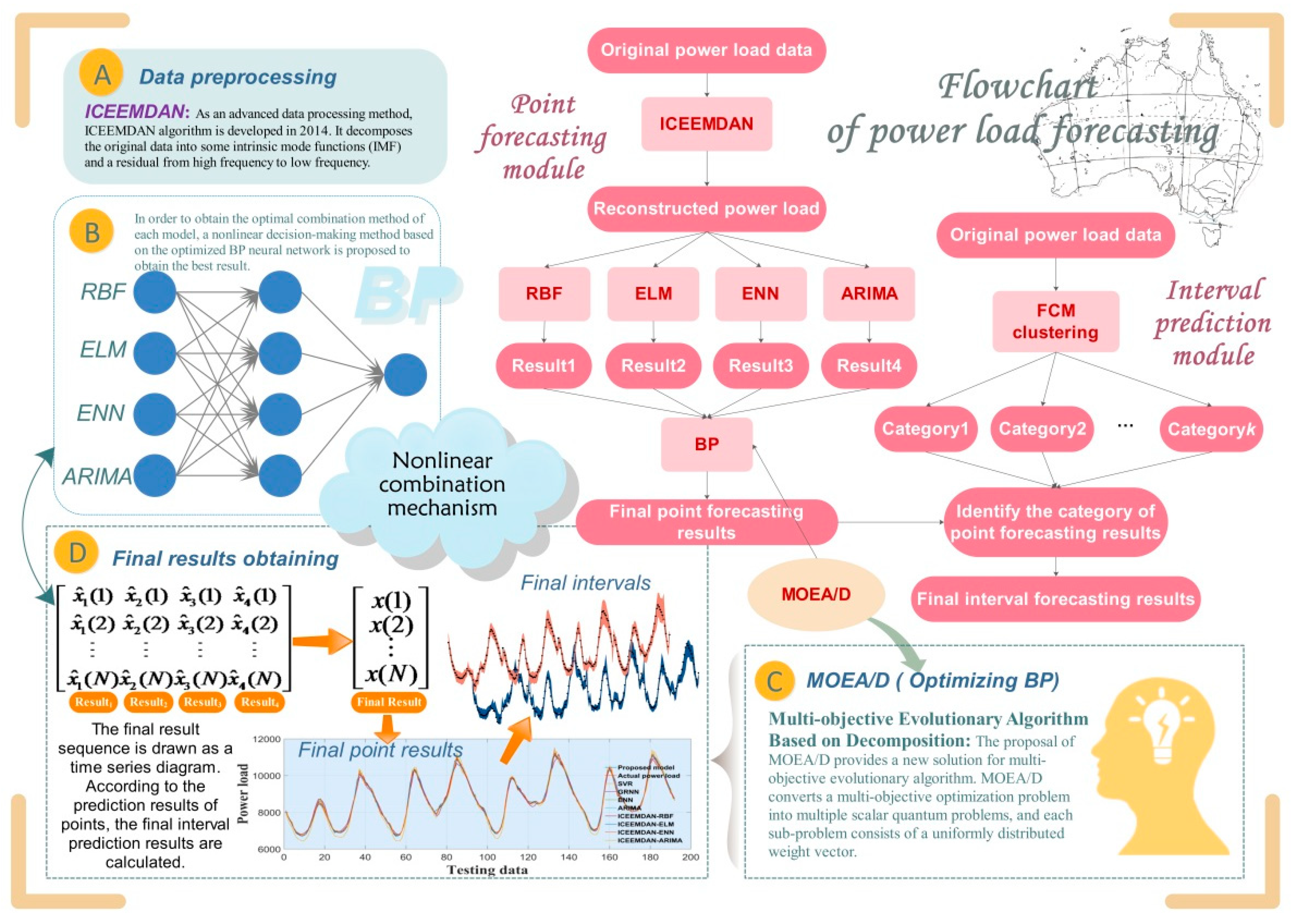
In this paper, a double forecasting system of power load is established. The double forecasting system means a forecasting system that integrates point forecasting and interval forecasting. The relationship between point forecasting and interval forecasting is similar to point estimation and interval estimation in statistics. The flow of the system we designed is to carry out point prediction first, get the result of point prediction, then construct a suitable confidence interval according to the result of point prediction to carry out interval prediction. The forecasting system includes two modules: point forecasting module and interval forecasting module. The following is the system construction process, and the system structure is shown in Figure 1.

3.1. Point Forecasting Module

In this section, we successfully put forward a new type of nonlinear hybrid point forecasting model, using RBF, ELM, ENN and ARIMA, as well as BP network, MOEA/D algorithm and nonlinear combination mechanism to achieve high-precision and more stable load point prediction results. Considering the good prediction performance of BP network, this paper takes BP network as the method of nonlinear combination.

The point prediction module of the designed system is composed of four steps. The details are as follows:

Step 1: Power load data preprocessing.

For the sake of removing the noise and further collect helpful information from the power load sequence, we use ICEEMDAN technology to disintegrate the original sequence, and rebuild the smooth time series. Specifically, the original sequence is decomposed into some IMFs. IMFs with higher frequency are eliminated to filter the time series. Here we remove IMF₁, and the remaining IMFs are rebuilt to get the final series.

Step 2: Single model predicting.

In this study, we first use single models to predict the points to obtain a preliminary impression of each model. Then the higher prediction accuracy model, RBF, ELM, ENN and ARIMA, are chosen as member prediction models to build the combination model. RBF, ELM and ENN are used to handle the non-linear features of load, while ARIMA has a good effect on discerning linear characteristics of load data. Say concretely, we divide 1488 load data into training set train and testing set test, where train includes 1152 data and test includes 336 data. The rolling forecasting strategy is employed, which adopts the original data of the previous five periods to forecast the next period. The input and output structure of train is shown in Equations (14) and (15). Using the RBF, ELM and ENN which trained by train to predict the load of the testing set, the prediction sequences predict₁, predict₂ and predict₃ are obtained, respectively. Similarly, ARIMA is used to obtain the prediction sequence. predict_i (i = 1,…,4), including 336 forecasting values are taken as the input datasets, which are inputted into the BP model.

$$inpu{t}_1=\left[\begin{array}{cccc}x(1)& x(2)& \cdots & x(l)\\ x(2)& x(3)& \cdots & x(l+1)\\ ⋮& ⋮& \ddots & ⋮\\ x(n-l)& x(n-l+1)& \cdots & x(n-1)\end{array}\right]$$

(14)

$$outpu{t}_1=\left[\begin{array}{c}x(l+1)\\ x(l+2)\\ ⋮\\ x(n)\end{array}\right]$$

(15)

In the Equations (14) and (15), n is the number of train and l is look-back time lag, and x(k) is the power load value at time k. For example, take x(1) to x(l) as input and x(l + 1) as output; next, take x(2) to x(l + 1) as input and x(l + 2) as output, to train the structure of RBF, ELM and ENN. Here, we set l = 5.

Step 3: Nonlinear combination model constructing.

For the sake of obtaining the combination model, a nonlinear decision-making method on the basis of BP neural network optimized by MOEA/D is proposed to achieve the best result.

Before introducing the nonlinear integration, the linear integration method is first introduced. Linear integration is to sum up the prediction results by linear weighting the prediction results of n single prediction models. Suppose y_t is the actual value, predict_it (i = 1, 2, ..., n) is the prediction result at time t, and n is the number of prediction models. w_i represents the weight of the i-th prediction model, and ${\displaystyle {\sum }_{i=1}^n{w}_i=1}$. Therefore, the final prediction results can be calculated as follows

$${\widehat{y}}_t={\displaystyle {\sum }_{i=1}^n{w}_{i}predic{t}_{it}},\begin{array}{c}\end{array}t=1,2,\dots ,m$$

(16)

Considering the complexity of power load and the characteristic of different single models, we choose nonlinear weight combination forecasting to compensate for the shortage of linear integration. In this study, as an important application of nonlinear integration, BP is applied to the integration of a single prediction component for final prediction. Specially, BP neural network is a complex nonlinear black box operation, and a large number of internal nodes in it are connected with each other, which can be used as an arbitrary function approximation mechanism. We regard the trained BP neural network as the weight integration of each single model, so this combination weight can also be regarded as nonlinear integration. However, BP parameters have an important impact on the prediction results and it is difficult to determine. Therefore, as an advanced swarm intelligence algorithm, MOEA/D is used to improve BP parameters to improve forecasting performance.

In particular, the predict₁, predict₂, predict₃ and predict₄, which contains 336 power load prediction values obtained from the RBF, ELM, ENN and ARIMA models mentioned in Step 2, are the basic data of the BP model, where the first 240 values are considered as the training set and the remaining 96 values are taken as the testing set. Then the 96 prediction values obtained by BP are the forecasting results of our proposed model. It is worth noting that it is difficult to find the weights and thresholds of neurons in each layer of BP network, so MOEA/D is introduced to search for the best weights and thresholds of neural network, which solves this problem to a certain extent. The input and output structure of BP network training is shown in Equations (17) and (18).

$$\begin{array}{l}inpu{t}_2=\left[\begin{array}{ccc}predic{t}_1& predic{t}_2& \begin{array}{cc}predic{t}_3& predic{t}_4\end{array}\end{array}\right]\\ \begin{array}{cccc}\begin{array}{cc}& \end{array}& & & \end{array}=\left[\begin{array}{cccc}{\widehat{x}}_1(1)& {\widehat{x}}_2(1)& {\widehat{x}}_3(1)& {\widehat{x}}_4(1)\\ {\widehat{x}}_1(2)& {\widehat{x}}_2(2)& {\widehat{x}}_3(2)& {\widehat{x}}_4(2)\\ ⋮& ⋮& ⋮& ⋮\\ {\widehat{x}}_1(N)& {\widehat{x}}_2(N)& {\widehat{x}}_3(N)& {\widehat{x}}_4(N)\end{array}\right]\end{array}$$

(17)

$$outpu{t}_2={\left[\begin{array}{cccc}x(1)& x(2)& \cdots & x(N)\end{array}\right]}^T$$

(18)

In which N is 336, and ${\widehat{x}}_1(k),{\widehat{x}}_2(k),{\widehat{x}}_3(k),{\widehat{x}}_4(k)$ is the k-th load value predicted by RBF, ELM, ENN and ARIMA, respectively. By input and output, the optimized BP neural network can be trained.

Step 4: Power load point prediction.

According to the established nonlinear prediction model, the rolling forecasting technique is applied for multi-step forecasting, and the final prediction results are obtained. The evaluation index is calculated by using the prediction result and test, and then the performance of the model is effectively evaluated.

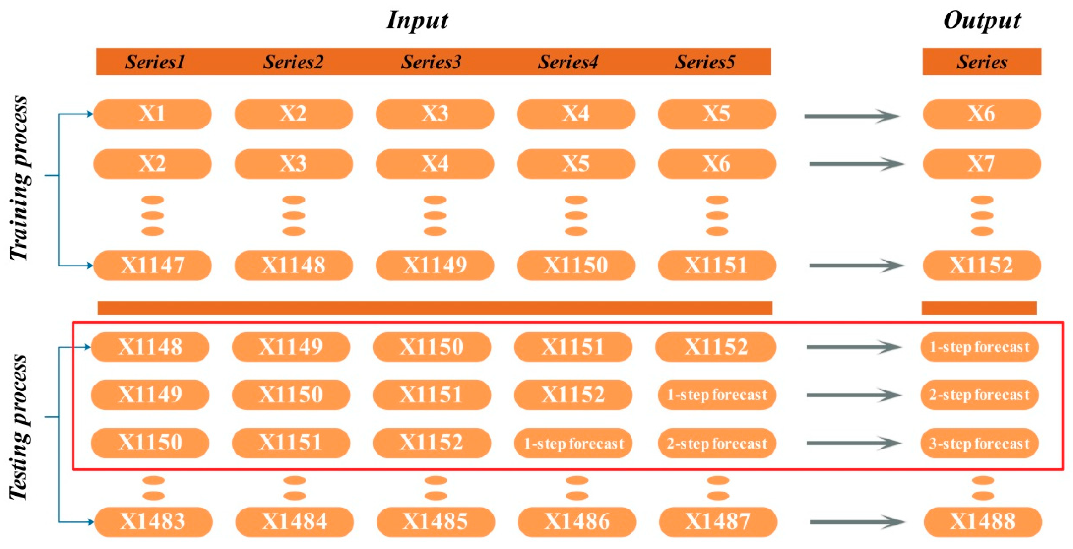
Specially, multi-step forecasting means forecasting multiple load values in the future. A time index t is the forecast origin and a positive integer l is the forecast horizon. It can be assumed that the time index t is exactly the time point that we are in, and our target is to obtain the forecasting value ${\widehat{y}}_{t+l}$(l ≥ 1). l = 1,2,3 corresponds to 1-step, 2-steps and 3-steps, respectively. Figure 2 shows the data usage of multi-step forecasting.

3.2. Interval Forecasting Module

Interval forecasting is obtaining the value interval of future load by certain forecasting methods, which shows the possible fluctuation range of future load. If accurate load point prediction can guarantee the daily operation of power grid, then effective interval prediction can further quantify the uncertainty of power load and provide reliable and accurate load information. The interval forecasting method of this system is developed according to point prediction, which is an interval prediction method based on fuzzy system. The principle of the interval forecasting method proposed in this study is to classify the point forecasting results according to different kinds of load data and construct different but adaptive intervals. The classification is based on the real load data, and judge which category the prediction results belong to, and then construct a specific confidence interval for this category, so as to get the predicted load interval. The three steps of interval forecasting module are shown as:

Step 1: Data classification.

The training set train of load data is clustered into several classes by FCM clustering method. Assume that the data in each category follows the same normal distribution. Therefore, we can get some interval classes $F_1,F_2,\cdots ,F_k$. The mean value and variance of each category are calculated respectively to prepare for the interval construction next.

Step 2: Load interval estimation.

The confidence degree of each category interval is 95%. According to the mean and variance of each category data, the corresponding confidence interval is constructed. Different categories have different width of unified prediction interval. This process of constructing different adaptive intervals according to different data characteristics is also one of the innovations of this model. According to the testing set test point prediction results in the point prediction module, identify the category F that each prediction value falls into. Then, according to the constructed confidence interval of each category, the prediction interval of each prediction value is calculated as:

$$[x_i-z_{1-\alpha /2}\frac{s_j}{\sqrt{n_j}},x_i+z_{1-\alpha /2}\frac{s_j}{\sqrt{n_j}}]$$

(19)

where x_i is point prediction value, j is the category number of x_i, s_j is standard deviation of category j, n_j is the data number of category j.

Step 3: Sorting out the prediction results.

According to the prediction interval of the above points, the final interval estimation of the power load is obtained.

4. Experiments and Analysis

This section introduces the application of the double forecast model and several comparison models, and divides the comparison into three experimental demonstrations. The operating environment of the experiment is: 2.60 GHz CPU, 4.00 GB RAM, Windows 7 and Matlab R2016A. Considering the random factors, to guarantee the reliability of the final results, 20 experiments are carried out each time, and the average value is taken, respectively.

4.1. Dataset Description

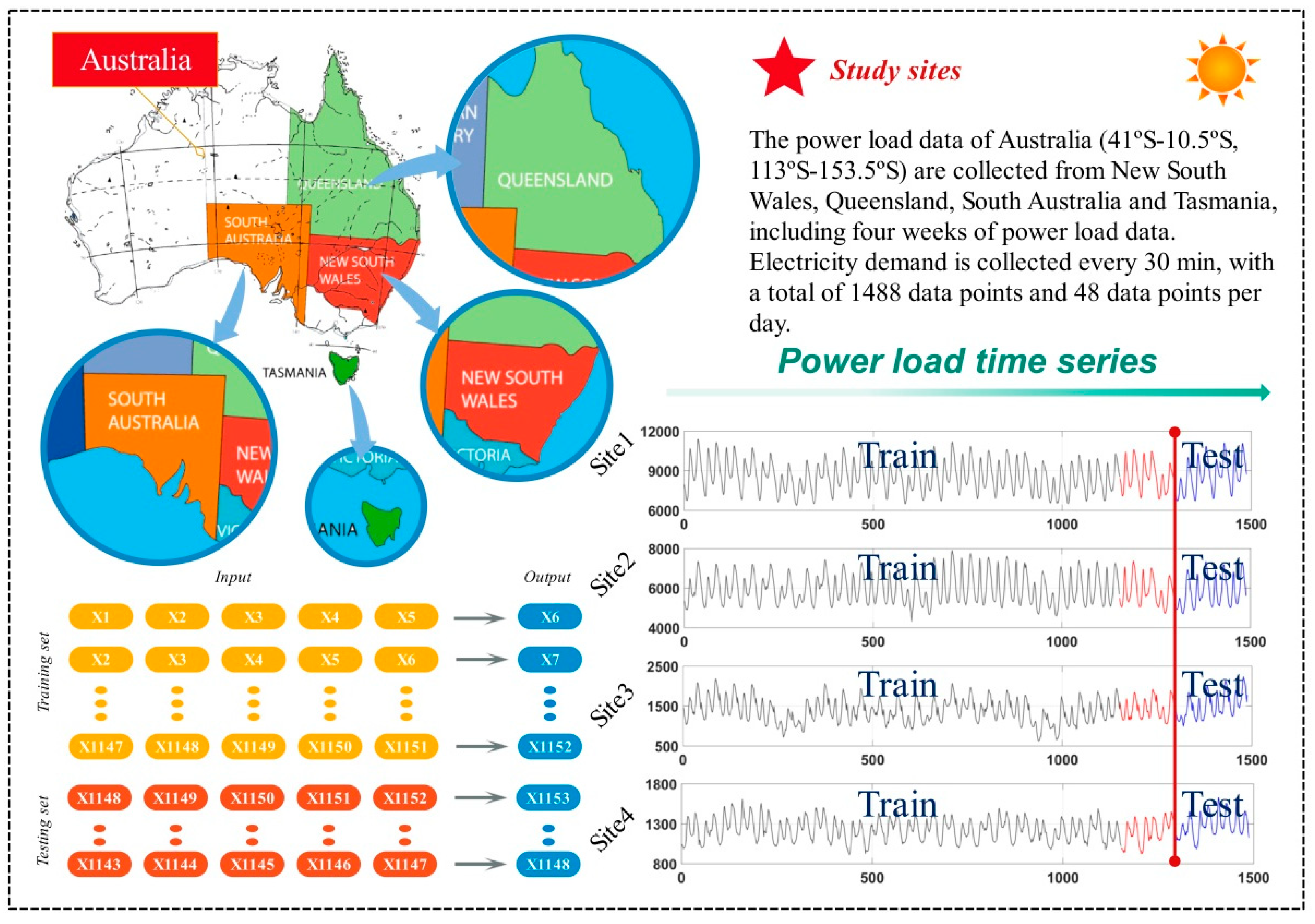
From July 1, 2019 to July 31, 2019, power load data were collected from New South Wales, Queensland, South Australia and Tasmania, including four weeks of power load data in this paper. Electricity demand is collected every 30 min, with a total of 1488 data points and 48 data points per day. Among them, the data from July 1, 2019 to July 27, 2019 were chosen as training set of selected model, 27 days in total, including 1296 data points; the data from July 28, 2019 to July 31, 2019 were used as testing set, 4 days in total, including 192 data points. At the same time, the last three days data are used to decide the network structure of BP model. Training set and testing set select identical rolling forecasting technique and output one-step, two-step and three-step prediction results. The power load data from July 1, 2019 to July 31, 2019 and its statistical indicators which are minimum, maximum, mean and std., are shown in

Table 2. Structure of four selected datasets in Australia.

Site	Samples	Numbers	Statistical Indicator
			Mean	Std.	Max	Min
Site 1	All samples	1488	8568.51	1124.32	11379.76	6372.63
	Training	1296	8556.83	1114.88	11379.76	6372.63
	Testing	192	8647.37	1186.12	11107.04	6697.94
Site 2	All samples	1488	5935.55	738.00	7884.64	4318.74
	Training	1296	5954.18	737.86	7884.64	4318.74
	Testing	192	5809.81	728.39	7337.13	4707.27
Site 3	All samples	1488	1395.97	296.05	2229.02	611.41
	Training	1296	1379.04	292.24	2178.39	611.41
	Testing	192	1510.24	297.05	2229.02	997.92
Site 4	All samples	1488	1231.81	138.65	1628.73	910.65
	Training	1296	1223.45	135.83	1611.11	910.65
	Testing	192	1288.19	144.56	1628.73	987.02

Power load of New South Wales, Queensland, South Australia and Tasmania from 1 July to 31 July 2019.

. The distribution condition of areas and dataset are presented in Figure 3.

As shown in the Table 2, the statistics of all samples, training sets and testing sets of three sites are similar. The data set is reasonable and can be chosen to testify the supreme ability of the proposed model.

4.2. System Evaluation

The evaluation indexes of the designed double prediction system are introduced, including 5 indexes of point prediction and 4 indexes of interval prediction.

4.2.1. Point Forecasting Evaluation

Generally speaking, the evaluation criteria are not unique for the prediction system. Hence, this paper uses five common evaluation standards to assess the point forecasting performance of the proposed model and other comparative models. The five indexes include mean absolute percentage error (MAPE), root mean square error (RMSE), mean absolute error (MAE), direction change (DC) and the index of agreement of forecasting results (IA). Among these indexes, the smaller the values of MAPE, RMSE and MAE, the larger the values of DC and IA, the better the prediction performance. See

Table 3. Point forecasting evaluation metrics.

Indicator	Definition	Equation
MAPE	Mean Absolute Percentage Error	$\mathbf{MAPE}=\frac{1}{N}{\displaystyle \sum _{i=1}^N\left|\frac{y_i-{\widehat{y}}_i}{y_i}\right|}\cdot 100\%$
MAE	Mean Absolute Error	$\mathbf{MAE}=\frac{1}{N}{\displaystyle \sum _{i=1}^N|y_i-{\widehat{y}}_i|}$
RMSE	Root Mean Square Error	$\mathbf{RMSE}=\sqrt{\frac{1}{N}\cdot {\displaystyle \sum _{i=1}^N{(y_i-{\widehat{y}}_i)}^2}}$
DC	Directional Change	$\mathbf{DC}=\frac{100}{N-1}{\displaystyle \sum _{t=1}^{N-1}{a}_t}$
IA	Index of agreement	$\mathbf{IA}=1-{\displaystyle {\sum }_{i=1}^N{(y_i-{\widehat{y}}_i)}^2}/{\displaystyle {\sum }_{i=1}^N{(|{\widehat{y}}_i-\overline{y}|-|y_i-\overline{y}|)}^2}$

Among the formula, $y_i$ and ${\widehat{y}}_i$ is the true and predicted value. N represents the testing set number. In addition, a_i is the directional factor, and is calculated as $a_t=\{\begin{array}{cc}0,& otherwise\\ 1,& if((y(t+1)-y(t))(\widehat{y}(t+1)-y(t)))>0\end{array}$.

for details of the four indicators.

4.2.2. Interval Forecasting Evaluation

For interval prediction, we select four evaluation indexes, which are forecasting interval coverage probability (FICP), forecasting interval normalized average width (FINAW), mean width of the constructed PIs (MPI) and Accumulated width deviation (AWD).

Table 4. Interval prediction evaluation metrics.

Indicator	Definition	Equation
FICP	Forecasting interval coverage probability	$\mathbf{FICP}=\frac{1}{N}{\displaystyle \sum _{i=1}^N{c}_i\times 100\%}$
FINAW	Forecasting interval normalized average width	$\mathbf{FINAW}=\frac{1}{N}{\displaystyle \sum _{i=1}^N\frac{U_i-L_i}{y_{\max }-y_{\min }}\times 100\%}$
MPI	Mean width of the constructed PIs	$\mathbf{MPI}=\frac{1}{N}{\displaystyle \sum _{i=1}^N|U_i-L_i|}$
AWD	Accumulated width deviation	$\mathbf{AWD}=\frac{1}{N}{\displaystyle \sum _{i=1}^N{\mathbf{AWD}}_i}$

Among the formula, U_i and L_i represent the upper limit and lower limit of forecasting interval, respectively. c_i is the number of the truth value contained in constructed interval. N represents the testing set number. y_max and y_min are the maximum and minimum of the targets in the whole prediction process. In addition, the calculation expression of AWD_i is $\mathbf{AWD}=\frac{1}{N}{\displaystyle \sum _{i=1}^N\mathbf{A}\mathbf{W}{\mathbf{D}}_i}$, and AWD_i is the width deviation of construction interval of each sample.

shows the specific definitions of four indices.

Specifically, FICP is the forecasting interval coverage probability of the test data set, which is the main evaluation index of interval prediction. It indicates the coverage effect of the obtained confidence interval to the actual value. Given the confidence level, if FICP is at least greater than or equal to 1-alpha, the constructed interval is valid; otherwise, the constructed interval is invalid. FINAW is the normalized average width of the forecasting interval of the testing set. The cost of reducing the width is diminishing the possibility of expected target covering; increasing the coverage requires increasing the width of the interval, so FICP and FINAW are essentially contradictory. MPI represents the average width of the obtained interval. AWD is the accumulated width deviation of testing dataset, which could be obtained by calculating the relative deviation degree. The cumulative sum of AWD_i can measure the relative deviation degree. See Table 4 for the specific description of the formula.

4.3. Diebold-Mariano Test

To verify the designed hybrid model owns better forecasting ability than compared models, an effective verification method called Diebold-Mariano (DM) test proposed by Diebold FX and Mariano RS is adopted. The theory of DM test is introduced first.

Considering the significance level $\alpha$, zero hypothesis H₀ indicates the predictive effectiveness of the developed model and the comparison model are not significantly different. The meaning of H₁ is contrasted with H₀. The relevant formulas are shown as:

$${\mathrm{H}}_0:\mathit{E}[\mathit{L}(\mathit{e}\mathit{r}{\mathit{r}}_i^1)]=\mathit{E}[\mathit{L}(\mathit{e}\mathit{r}{\mathit{r}}_i^2)]$$

(20)

$${\mathrm{H}}_1:\mathit{E}[\mathit{L}(\mathit{e}\mathit{r}{\mathit{r}}_i^1)]\ne \mathit{E}[\mathit{L}(\mathit{e}\mathit{r}{\mathit{r}}_i^2)]$$

(21)

In the formula, L represents the loss function of prediction error. err_i¹ and err_i² are the error sequence predicted by selected model.

In addition, the statistics of DM test can be defined in the following ways:

$$\mathrm{DM}=\frac{{\displaystyle {\sum }_{i=1}^n(\mathit{L}(\mathit{e}\mathit{r}{\mathit{r}}_i^1)-\mathit{L}(\mathit{e}\mathit{r}{\mathit{r}}_i^2))}}{\sqrt{S^2/n}}{s}^2$$

(22)

in which S² is the estimate of the variance of $d_i=\mathit{L}(\mathit{e}\mathit{r}{\mathit{r}}_i^1)-\mathit{L}(\mathit{e}\mathit{r}{\mathit{r}}_i^2)$. Assuming a certain significance level $\alpha$, the obtained value DM is in comparison with that of $z_{\alpha /2}$. Once DM statistics exceed the interval [$-z_{\alpha /2}$,$z_{\alpha /2}$], H₀ can be rejected. This shows the predictive performance of the established model and that of the comparative model are significantly different, which means that H₁ will be accepted.

4.4. Results and Analysis of Point Forecasting

To testify the performance of the point prediction module, two experiments are conducted in this part: experiment I and experiment II. The main purpose of experiment I is to prove the good ability of the nonlinear combination model in the point forecasting, so as to reasonably verify the superiority of the proposed model. In addition, experiment I proves the necessity of data preprocessing. In the same way, to prove the rationality and superiority of the ICEEMDAN technology selected in this work, it is compared with other commonly used data preprocessing technology, and this is the content of experiment II. The detailed analysis of each experiment is as follows.

4.4.1. Experiment I: Comparison with Individual Models

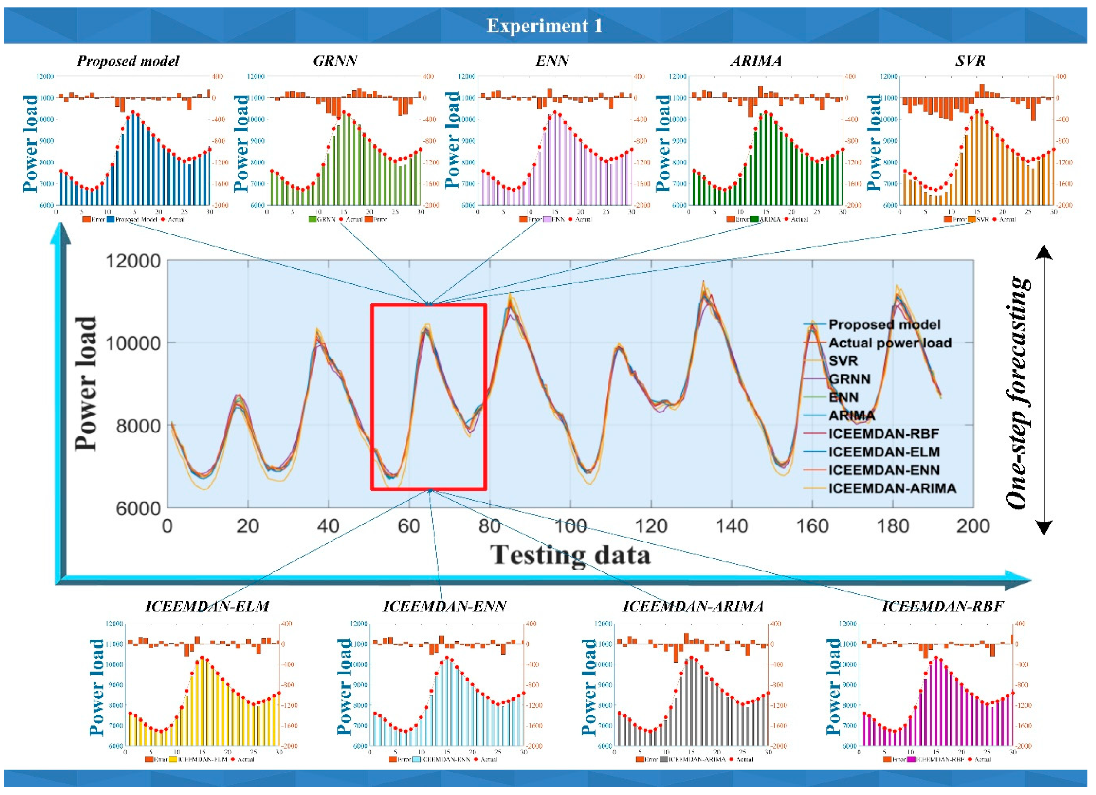
In this work, all experimental datasets are trialed to assess the effectiveness of the point prediction module, while three comparisons are designed. In comparison (a), the proposed model is compared with the four data preprocessed models, ICEEMDAN-RBF, ICEEMDAN-ELM, ICEEMDAN-ENN and ICEEMDAN-ARIMA, in order to analyze the advantages of the combination model using the nonlinear combination method. In comparison (b), four ICEEMDAN-based models are compared with single models RBF, ELM, ENN and ARIMA, respectively. In comparison (c), the effectiveness of the designed forecasting model is further tested by using the traditional model SVR and Generalized Regression Neural Network (GRNN) as comparison methods. The predicted results are displayed in

Table 5. Abilities of the established model and single models.

Site	Model	One-Step					Two-Step					Three-Step
		MAPE	MAE	RMSE	IA	DC	MAPE	MAE	RMSE	IA	DC	MAPE	MAE	RMSE	IA	DC
Site 1	SVR	1.9099	156.7013	187.9195	0.9944	0.8220	2.5219	210.3356	258.5180	0.9894	0.7474	3.0868	262.8112	341.3188	0.9817	0.6614
	GRNN	1.2373	107.3457	140.2939	0.9964	0.9215	2.1193	183.9606	244.3408	0.9885	0.8632	3.1821	276.0676	368.4048	0.9727	0.7778
	RBF	1.3330	120.0048	162.0430	0.9951	0.9058	2.5730	227.8929	303.8217	0.9819	0.8053	5.7891	518.6760	671.9120	0.8625	0.6143
	ELM	0.8640	75.3729	101.7329	0.9981	0.9476	2.8427	246.4113	327.8275	0.9733	0.8304	6.0739	518.3696	663.3588	0.9629	0.7570
	ENN	0.9387	81.4666	108.1564	0.9979	0.9476	2.1680	188.5787	247.6781	0.9886	0.8053	3.4611	299.2232	375.4925	0.9727	0.6614
	ARIMA	1.2105	103.8960	137.7456	0.9965	0.9058	2.5009	224.8970	300.2767	0.9839	0.7526	2.4838	223.0066	292.3059	0.9847	0.7672
	ICEEMDAN-RBF	0.7367	65.4730	94.1611	0.9984	0.9476	2.2596	198.6571	278.7425	0.9862	0.8368	5.2163	471.4579	1091.9532	0.8148	0.7937
	ICEEMDAN-ELM	0.8543	74.4721	98.4847	0.9983	0.9424	2.7422	239.9533	319.7560	0.9810	0.7579	5.6887	494.3489	636.1800	0.9215	0.6190
	ICEEMDAN-ENN	0.9216	81.0992	105.1646	0.9980	0.9319	1.8371	159.6742	204.5202	0.9923	0.8579	3.0383	261.0713	330.9170	0.9788	0.6984
	ICEEMDAN-ARIMA	1.0649	94.4410	123.4999	0.9973	0.9267	2.3297	209.7987	281.9299	0.9857	0.7895	2.3985	215.6049	282.7638	0.9856	0.7831
	Proposed Model	0.6577	56.7791	80.1018	0.9988	0.9372	1.6540	143.5974	192.1716	0.9932	0.8474	1.7361	151.6523	200.2943	0.9926	0.8730
Site 2	SVR	3.6548	212.2143	250.9721	0.9780	0.6754	3.8775	228.6832	273.7403	0.9737	0.6368	3.5513	208.0377	261.8331	0.9734	0.6085
	GRNN	1.5213	86.3305	117.6754	0.9932	0.8377	2.3967	135.6083	189.3953	0.9822	0.6947	3.3451	188.7230	274.1698	0.9618	0.6508
	RBF	0.9823	58.2252	76.4982	0.9973	0.9058	3.3178	195.5145	263.8302	0.9576	0.7862	7.1590	416.3507	603.8911	0.6753	0.4778
	ELM	0.9063	53.5149	68.9417	0.9977	0.9058	2.9227	170.9014	228.5369	0.9705	0.8253	6.0964	353.5843	484.5720	0.8766	0.6571
	ENN	1.0283	60.5118	80.1060	0.9969	0.9267	2.1192	125.0372	168.7274	0.9863	0.8053	3.5815	209.5433	279.5027	0.9611	0.6667
	ARIMA	2.2121	125.7167	146.7645	0.9901	0.7487	2.4574	146.4694	189.3542	0.9830	0.7368	2.4456	146.0298	189.5241	0.9830	0.7407
	ICEEMDAN-RBF	0.9729	57.3546	80.5129	0.9969	0.8901	3.1682	185.6588	279.8124	0.9639	0.7263	7.2699	412.7709	950.5817	0.6926	0.5661
	ICEEMDAN-ELM	0.8875	52.5323	66.6224	0.9979	0.9110	2.8790	169.0021	227.7103	0.9755	0.7368	5.8342	340.6032	450.3827	0.9043	0.6349
	ICEEMDAN-ENN	0.9815	58.7002	77.6269	0.9971	0.9005	1.9832	115.6628	155.7612	0.9882	0.8526	3.1668	183.2636	247.5578	0.9692	0.7354
	ICEEMDAN-ARIMA	1.0105	60.3096	79.7003	0.9970	0.8848	2.3534	139.8655	181.7611	0.9842	0.7737	2.3018	136.8617	181.2463	0.9843	0.7672
	Proposed Model	0.7373	43.3423	55.6332	0.9985	0.9319	1.8561	110.1146	146.8969	0.9893	0.8000	1.8413	109.4865	144.4127	0.9897	0.8307
Site 3	SVR	18.1694	250.6877	267.6887	0.8619	0.5759	16.2465	226.7004	250.1855	0.8711	0.5842	14.4738	204.6135	234.3931	0.8790	0.5503
	GRNN	3.4558	53.6071	71.4746	0.9838	0.7330	5.9445	93.0097	121.8883	0.9503	0.5368	8.4107	133.1739	176.0579	0.8896	0.4709
	RBF	4.7792	72.5550	105.3551	0.9017	0.7671	15.8938	241.5826	305.6250	0.8735	0.5163	18.0374	270.8042	333.5527	0.8372	0.3619
	ELM	2.5036	38.1800	53.4851	0.9917	0.8482	4.5972	69.6088	90.9124	0.9746	0.5895	6.8086	102.6562	132.6552	0.9411	0.4233
	ENN	2.5906	39.5491	54.8027	0.9912	0.8168	5.2533	80.6505	109.2907	0.9626	0.5684	8.0953	123.4767	165.8262	0.9066	0.4550
	ARIMA	3.3119	50.7776	66.8833	0.9860	0.7539	4.6843	69.4605	98.5552	0.9721	0.6947	4.6833	69.4314	98.7034	0.9722	0.6984
	ICEEMDAN-RBF	4.1722	70.1981	187.8232	0.9075	0.8010	15.8023	220.4719	256.5942	0.8629	0.5947	16.2465	226.7004	250.1855	0.8711	0.5842
	ICEEMDAN-ELM	2.2105	33.5601	51.5923	0.9922	0.8848	7.0790	108.0376	149.7840	0.9297	0.4737	12.7588	193.4990	266.7974	0.7656	0.4233
	ICEEMDAN-ENN	2.4307	37.2182	53.8956	0.9914	0.8272	4.9206	75.8476	99.2984	0.9693	0.5632	7.2839	112.3960	147.7066	0.9259	0.4233
	ICEEMDAN-ARIMA	2.4481	36.6852	53.6428	0.9917	0.8482	4.4250	66.3791	90.2881	0.9760	0.6895	4.4222	66.5045	90.6995	0.9759	0.6931
	Proposed Model	2.0714	30.9618	44.2547	0.9945	0.8691	3.6063	54.3514	75.7387	0.9828	0.7474	3.7028	54.7373	72.0933	0.9847	0.7720
Site 4	SVR	3.9387	49.3677	54.0031	0.9679	0.6440	5.4554	70.1198	78.7384	0.9284	0.5789	4.4034	56.5173	70.1077	0.9426	0.6296
	GRNN	1.6749	22.1333	30.1784	0.9881	0.8482	2.6568	35.3348	47.6012	0.9683	0.6895	3.6258	48.2613	63.0378	0.9402	0.6243
	RBF	2.7267	168.5272	237.3737	0.9866	0.7898	4.9468	289.4248	391.8644	0.9526	0.7295	9.3387	429.3665	579.0957	0.9044	0.6844
	ELM	1.4988	19.6842	26.1392	0.9919	0.8264	4.1464	55.3052	77.8929	0.9656	0.7295	8.0347	107.8908	151.7349	0.9279	0.6481
	ENN	1.5777	20.7727	27.2960	0.9908	0.8220	3.0841	41.0474	56.3762	0.9578	0.6526	4.6071	61.4170	83.6801	0.8986	0.6138
	ARIMA	1.7759	23.5059	31.3690	0.9873	0.8063	2.7463	36.2074	48.6230	0.9715	0.7105	2.7533	36.3150	48.6865	0.9714	0.7143
	ICEEMDAN-RBF	2.5025	208.7714	257.0299	0.9895	0.7474	4.7572	285.1412	335.2767	0.9597	0.5579	8.9365	489.6447	531.0756	0.9060	0.5947
	ICEEMDAN-ELM	1.3761	18.0908	23.9922	0.9927	0.8429	4.1208	54.6678	72.7303	0.9247	0.6526	7.4296	98.1502	129.9749	0.7542	0.6032
	ICEEMDAN-ENN	1.5181	20.0772	27.7423	0.9904	0.8168	2.6237	34.9796	47.8112	0.9694	0.7000	3.7543	50.2631	68.4913	0.9304	0.6296
	ICEEMDAN-ARIMA	1.4191	18.5971	24.4587	0.9927	0.8115	2.5278	33.4552	46.0766	0.9740	0.6947	2.5401	33.6274	46.1556	0.9739	0.6931
	Proposed Model	1.3288	17.3109	22.2651	0.9939	0.8325	2.1116	27.1452	35.1427	0.9845	0.7474	2.2401	29.2987	39.5900	0.9806	0.7249

and Figure 4, and the comparison consequences are as follows.

(1) For comparison (a), the developed hybrid nonlinear model has the best ability in one to three step load forecast in four datasets, whose error index was superior to other models. For instance, in one-step forecasting, the MAPE of the established model is about 0.6577%, 0.7373%, 2.0714% and 1.3288%, while the prediction accuracy of the other ICEEMDAN-based model is 0.1% to 2% lower than that of the established model. For the two and three step prediction, the proposed model is also better than other models in four sites.

(2) For comparison (b), comparing ICEEMDAN-ENN and ICEEMDAN-ARIMA models with ARIMA and ENN without data preprocessing, it can be found that data preprocessing is very important to enhance the ability of load forecasting. For site 1, the MAPE of ENN and ARIMA are higher than that of ICEEMDAN-ENN and ICEEMDAN-ARIMA in one, two and three step prediction. The accuracy of ICEEMDAN-RBF and ICEEMDAN-ELM which are not shown in the table are also improved. For site 2, site 3 and site 4, and Figure 4, the situation is similar.

(3) For comparison (c), it can be seen from five indexes MAPE, MAE, RMSE, IA and DC of Table 5, the proposed model is more accurate than other individual models, such as SVR and GRNN. In addition to the proposed hybrid prediction model, the single model with high prediction accuracy is ARIMA and ENN. Therefore, we choose ARIMA and ENN as the model used in combination models, and the same circumstance as RBF. ARIMA is a linear model, therefore it can show that the power load data has certain linear characteristics, so it is a wise choice to take ARIMA into account in the proposed model. Additionally, although the prediction accuracy of BP is not shown, the experimental results show that it has relatively good prediction effect, so BP is selected as the model used in nonlinear combination.

4.4.2. Experiment II: Tests of Data Preprocessing Methods

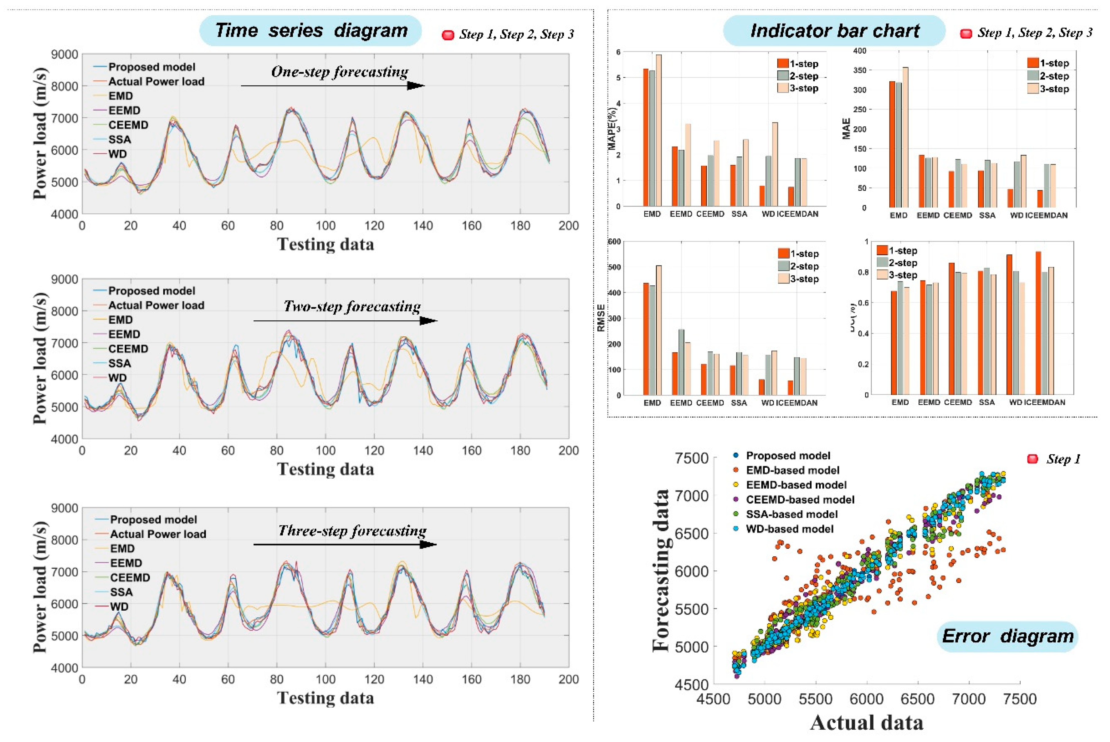
This experiment is aiming at comparing the effectiveness of ICEEMDAN selected in this system with other common data preprocessing methods, which includes EMD, EEMD, CEEMD, SSA and WD. Therefore, the point forecasting models on the basis of different data preprocessing methods are EMD-based model, EEMD-based model, CEEMD-based model, SSA-based model and WD-based model. These models only use different decomposition method in the data preprocessing stage. Through the experiment, we can test whether the proposed prediction model is reasonable, and can also find the best method to remove the noises to improve the prediction effectiveness.

The results obtained by models using different data preprocessing approaches are shown in

Table 6. The models with different data preprocessing techniques.

Site	Model	One-Step					Two-Step					Three-Step
		MAPE	MAE	RMSE	IA	DC	MAPE	MAE	RMSE	IA	DC	MAPE	MAE	RMSE	IA	DC
Site 1	EMD-based model	7.9921	703.2179	848.0034	0.7983	0.5916	8.0933	697.2798	827.3683	0.8112	0.5789	7.9109	691.9289	832.9187	0.8117	0.6190
	EEMD-based model	6.4768	550.6402	680.4857	0.8925	0.6178	7.0479	612.2662	730.6838	0.8657	0.6158	5.2011	459.5873	598.1909	0.9248	0.6561
	CEEMD-based model	2.0549	176.5654	227.7546	0.9904	0.8063	2.0285	175.3443	224.9582	0.9908	0.8211	2.1103	180.5625	228.8269	0.9901	0.7989
	SSA-based model	1.9070	168.8455	234.2489	0.9897	0.8586	1.9845	173.4462	231.2932	0.9901	0.8474	1.9283	168.1976	228.0082	0.9905	0.8677
	WD-based model	0.6582	57.0884	77.9511	0.9989	0.9529	1.7329	97.4880	132.7305	0.9968	0.9105	1.7491	152.1173	195.5254	0.9931	0.7989
	Proposed Model	0.6577	56.7791	80.1018	0.9988	0.9372	1.6540	143.5974	192.1716	0.9932	0.8474	1.7361	151.6523	200.2943	0.9926	0.8730
Site 2	EMD-based model	5.3342	320.8286	436.0318	0.8792	0.6754	5.2566	317.6441	426.5115	0.8853	0.7368	5.8824	356.6128	504.2290	0.8231	0.6984
	EEMD-based model	2.3126	133.3762	166.1339	0.9865	0.7435	2.1817	125.8414	255.6755	0.9881	0.7158	3.1988	127.6659	204.1506	0.9669	0.7302
	CEEMD-based model	1.5685	91.9520	121.0101	0.9930	0.8586	1.9680	122.0495	168.2834	0.9634	0.7968	2.5498	110.6276	159.9772	0.9730	0.7930
	SSA-based model	1.5960	93.8540	115.7924	0.9935	0.8063	1.9178	120.0527	167.5894	0.9763	0.8263	2.5884	112.8322	154.9322	0.9737	0.7824
	WD-based model	0.7946	46.7711	60.5276	0.9983	0.9110	1.9386	116.6306	157.2216	0.9834	0.8042	3.2482	132.8212	172.4281	0.9858	0.7302
	Proposed Model	0.7373	43.3423	55.6332	0.9985	0.9319	1.8561	110.1146	146.8969	0.9893	0.8000	1.8413	109.4865	144.4127	0.9897	0.8307
Site 3	EMD-based model	5.4613	85.9224	119.7561	0.9536	0.7382	5.1310	80.7809	107.1774	0.9643	0.7000	5.6913	89.9809	123.2727	0.9491	0.6931
	EEMD-based model	3.7079	55.8826	76.5499	0.9822	0.7906	4.0544	61.4638	79.3819	0.9809	0.7632	4.8349	76.8613	109.7442	0.9626	0.7037
	CEEMD-based model	3.9913	63.7212	106.0344	0.9649	0.8168	4.4234	69.8325	108.0533	0.9635	0.7632	4.6505	73.2335	109.6005	0.9625	0.7513
	SSA-based model	3.8344	57.2709	71.3412	0.9850	0.7749	4.1258	46.8649	59.0353	0.9898	0.8368	4.2619	59.1854	73.7429	0.9801	0.7989
	WD-based model	2.2001	33.1241	44.2224	0.9943	0.8743	4.4882	68.5368	93.9026	0.9730	0.6263	3.9055	58.9593	79.1266	0.9849	0.7460
	Proposed Model	2.0714	30.9618	44.2547	0.9945	0.8691	3.6063	54.3514	75.7387	0.9828	0.7474	3.7028	54.7373	72.0933	0.9847	0.7720
Site 4	EMD-based model	3.0164	164.0450	197.0500	0.9864	0.6649	2.4541	135.9545	177.9912	0.9885	0.6947	2.8497	158.4661	196.5824	0.9853	0.6825
	EEMD-based model	2.0505	112.7215	145.8150	0.9923	0.7853	2.3454	127.9509	166.0814	0.9897	0.7842	2.3412	126.2956	169.4155	0.9893	0.7725
	CEEMD-based model	1.4065	55.9504	77.3350	0.9978	0.9005	2.2781	125.7992	159.2066	0.9908	0.7368	2.3741	130.5010	164.7806	0.9901	0.6984
	SSA-based model	2.9273	158.8158	203.4684	0.9843	0.7487	2.5953	140.1998	191.1280	0.9863	0.7684	2.4590	136.6107	176.6479	0.9888	0.7143
	WD-based model	1.3885	18.2316	25.0351	0.9921	0.8377	2.1772	28.6344	38.9430	0.9805	0.7263	2.5671	30.6863	40.0557	0.9715	0.7072
	Proposed Model	1.3288	17.3109	22.2651	0.9939	0.8325	2.1116	27.1452	35.1427	0.9845	0.7474	2.2401	29.2987	39.5900	0.9806	0.7249

. Figure 5 shows a clearer and more intuitive comparison. The conclusion can be drawn that the model on the basis of the ICEEMDAN decomposition technology has much better performance than other decomposition based prediction models. Say concretely, for site 2, the MAPE value of ICEEMDAN-based proposed model is 0.7373%, 1.8561% and 1.8413% for three steps, which is 0.1 to 4 percentage points higher than that of EMD-based model, EEMD-based model, CEEMD-based model, SSA-based model and WD-based model. Of all the benchmark models, EMD-based model is the worst. Compared with other models, the MAE, RMSE, IA and DC of the one to three step prediction of the developed model are also improved to different extent, which further shows the superiority of the data preprocessing method selected by this hybrid model.

Remark 2.

Experiment I and experiment II focus on proving the advantages of the proposed point forecast module, and the results show that the designed point forecasting model is a very promising power load forecasting method. It can also prove that the combination of data preprocessing technology, optimization algorithm and nonlinear combined method could successfully solve the difficulties of load prediction through appropriate prediction methods.

4.5. Results and Analysis of Interval Prediction (Experiment III)

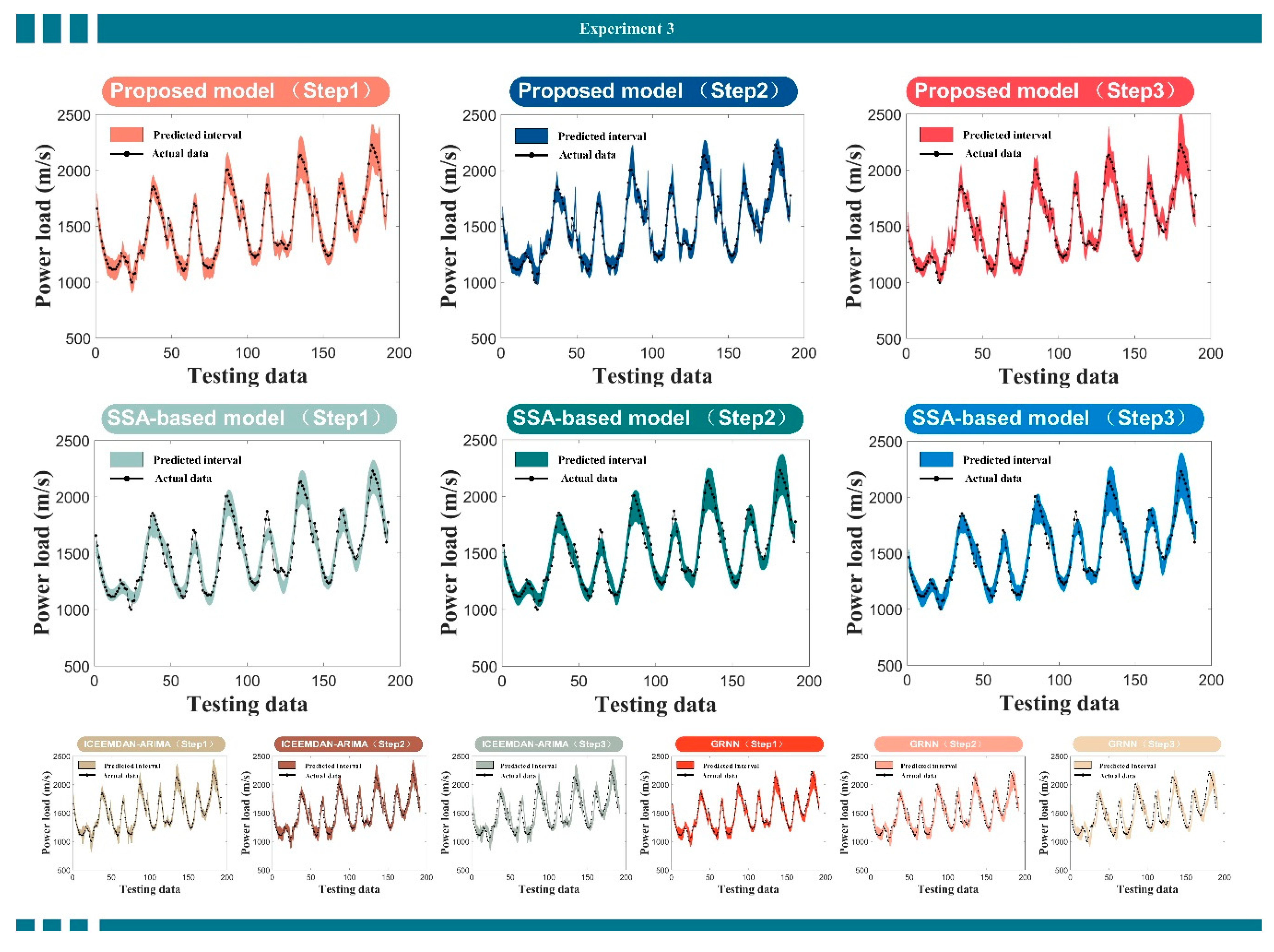
Base on the point power load forecasting, the probability interval forecasting could show more load information. In this part, we develop a method based on fuzzy clustering, which carries out interval forecasting on the basis of point forecasting. In addition, four datasets are applied in this experiment. To verifying the ability of the designed interval forecast module, we use the all the compared model of point prediction, and also use multi-step prediction to verify the interval predicted results. The results of the interval predicted model and other models are shown in

Table 7. The designed model comparing with all other models for site 2 and site 3.

Site	Model	One-Step				Two-Step				Three-Step
		FICP	FINAW	AWD	MPI	FICP	FINAW	AWD	MPI	FICP	FINAW	AWD	MPI
Site 2	SVR	0.5573	0.1383	0.1098	482.5648	0.5340	0.1327	0.1310	483.8663	0.6053	0.1313	0.1340	443.8932
	GRNN	0.8021	0.1288	0.0468	331.0903	0.6230	0.1270	0.1767	315.3002	0.5316	0.1246	0.2991	297.3550
	ENN	0.9479	0.1348	0.0055	363.8898	0.7592	0.1322	0.0725	366.4838	0.5421	0.1253	0.2361	339.8606
	ARIMA	0.9531	0.1314	0.0034	355.7632	0.6859	0.1297	0.0730	388.3355	0.7158	0.1283	0.0820	384.4358
	ICEEMDAN-RBF	0.9635	0.1296	0.0076	366.6068	0.6806	0.1257	0.1734	441.8282	0.5632	0.1008	0.3972	1005.4671
	ICEEMDAN-ELM	0.9896	0.1354	0.0005	364.4663	0.5916	0.1275	0.1506	407.4373	0.4526	0.1372	0.3171	520.7903
	ICEEMDAN-ENN	0.9740	0.1344	0.0035	355.5277	0.7330	0.1285	0.0844	351.9259	0.4737	0.1223	0.2831	339.3854
	ICEEMDAN-ARIMA	0.9583	0.1309	0.0037	354.3802	0.6649	0.1264	0.1009	387.4235	0.6842	0.1271	0.1005	389.6756
	EMD-based model	0.3750	0.1273	0.9095	281.9169	0.3560	0.1293	0.5799	269.8817	0.4053	0.1166	2.2804	300.4038
	EEMD-based model	0.6302	0.1301	0.1391	311.3577	0.6702	0.1294	0.1106	343.8937	0.7263	0.1397	0.1007	345.9396
	CEEMD-based model	0.8438	0.1388	0.0371	362.4171	0.8325	0.1355	0.0333	347.8779	0.8368	0.1382	0.0364	350.5409
	SSA-based model	0.8542	0.1377	0.0572	345.7467	0.8272	0.1368	0.0324	355.3823	0.8474	0.1396	0.0250	355.5278
	WD-based model	0.9844	0.1329	0.0002	349.5355	0.8220	0.1282	0.0344	342.3839	0.6632	0.1319	0.1068	333.2383
	Proposed Model	0.9896	0.1305	0.0002	356.9044	0.7906	0.1246	0.0587	333.2484	0.7895	0.1269	0.0554	355.3731
Site 3	SVR	0.1302	0.1320	1.0036	209.5036	0.1728	0.1296	0.9299	200.2102	0.2316	0.1361	0.7603	207.3294
	GRNN	0.6979	0.1327	0.0908	145.7429	0.4921	0.1355	0.3627	149.0968	0.3632	0.1349	0.7105	138.6840
	ENN	0.8490	0.1342	0.0582	169.3976	0.5654	0.1333	0.2129	163.6830	0.4632	0.1268	0.4586	155.3926
	ARIMA	0.8698	0.1389	0.0386	175.0206	0.6649	0.1272	0.1579	170.7487	0.6737	0.1251	0.1720	166.9475
	ICEEMDAN-RBF	0.8490	0.1094	0.1037	297.0992	0.7016	0.0004	0.1732	359.6531	0.6421	0.0010	0.3749	819.3448
	ICEEMDAN-ELM	0.9010	0.1368	0.0475	163.6025	0.4712	0.1354	0.3762	161.3793	0.2842	0.1214	0.8042	181.5007
	ICEEMDAN-ENN	0.8542	0.1298	0.0509	158.8348	0.5654	0.1290	0.2501	154.3947	0.4316	0.1343	0.5467	154.2944
	ICEEMDAN-ARIMA	0.8646	0.1383	0.0397	174.3103	0.7173	0.1319	0.1549	177.1593	0.7105	0.1330	0.1534	178.5047
	EMD-based model	0.5260	0.1354	0.2949	151.7276	0.5445	0.1436	0.2268	151.7952	0.5474	0.1390	0.2904	147.9657
	EEMD-based model	0.7448	0.1335	0.1169	158.3364	0.7068	0.1319	0.1259	146.1860	0.5842	0.1314	0.2563	137.7404
	CEEMD-based model	0.7396	0.1379	0.2067	150.0418	0.6963	0.1344	0.1944	156.7498	0.6632	0.1249	0.2152	149.5520
	SSA-based model	0.6458	0.1339	0.1313	145.7313	0.6806	0.1428	0.0744	158.4497	0.7211	0.1398	0.0708	159.1189
	WD-based model	0.9271	0.1338	0.0182	160.7955	0.6230	0.1337	0.1790	141.4222	0.7526	0.1250	0.1136	160.1570
	Proposed Model	0.9375	0.1319	0.0171	163.1146	0.6963	0.1304	0.1033	143.1301	0.7053	0.1300	0.1055	154.2024

. Due to the limited space, we only display the results of site 2 and site 3. We set the confidence interval to 90% to assess the effectiveness of the interval predicted model.

(1) For site 2, the best values of all indexes in all models are obtained by the proposed prediction model. For proposed model, the coverage probability of forecasting interval (FICP) is 98.96% in one-step, 79.06% in two-step and 78.95% in three-step. The average width of the interval is 356.9044, 333.2484 and 355.3731 in three steps according to MPI. Compared with the absolute value of power load, the interval width obtained is relatively accurate. AWD is 0.0002, 0.0587 and 0.0554 for three steps, shows the deviation degree of the constructed interval is small. All indexes reflect that the predicted interval of proposed model is qualified. In contrast, for the FICP of single prediction model, none of the predictions is better than proposed model. Although the ICEEMDAN-ELM has the same value of FICP as proposed model in one-step, it is largely lower than two and three-step.

(2) By combining FINAW with FICP, for the proposed model, when the FICP value is very high, FINAW is relatively small, which also shows the superiority of the developed model. In the one and two step forecast, the AWD of most other benchmark models is more than ten times of the developed model in one-step, and they are much larger in two and three step. This reflects the less deviation of the developed model. These four indexes fully reflect the superior forecasting ability of the developed model. The same conclusion can be drawn for site 3 in Table 7.

(3) At the same time, in order to intuitive show the comparison results, the results of the designed model and comparison models are pictured in Figure 6. The conclusions are consistent with Table 7, providing intuitive evidence for verifying the superior ability of the proposed system in the load interval forecasting. As shown in Figure 6, compared with other models, the proposed model has more accuracy interval forecast results. Obviously, the prediction range not only covers most of the load values, but also is narrowest among all models. This shows that the designed model is more stable than others. As a result, the designed model has greater advantages for three experimental datasets.

Remark 1.

The same as the comparison model used in point forecast, 13 different competition models based on four datasets and multi-step interval forecast are compared. The results show the designed interval model is better than all the comparison models. Due to the excellent ability of the designed interval prediction module based on fuzzy clustering, it is a very promising interval prediction method of power load.

5. Discussions

For the sake of discussing the experiment conclusions in detail and reduce the error of power load forecasting, the validity of the established model, the combination mechanism of combination model and the practical application in the power system are discussed.

5.1. DM Test

The validity of the model is verified by DM test by all other models comparing with the proposed hybrid forecasting model. Based on DM test theory, the zero hypothesis is that the prediction results of both models is no significant difference, while the alternative hypothesis is contrast. We chose two scales with alpha of 0.1 and 0.05 as the criteria to judge the significance of the results, among which Z_0.05/2 = 1.96 and Z_0.1/2 = 1.645.

Table 8. Statistics value of DM test for experimented models.

Model	Site 1			Site 2			Site 3			Site 4			Average
	1-Step	2-Step	3-Step	1-Step	2-Step	3-Step	1-Step	2-Step	3-Step	1-Step	2-Step	3-Step	1-Step	2-Step	3-Step
SVR	10.2421	3.7990	5.4450	12.0094	7.7489	6.6256	20.2303	14.8429	13.6510	15.4262	11.4861	7.2714	14.4770	9.4692	8.2482
GRNN	6.7005	2.7004	6.3344	5.8339	2.6935	4.5938	5.1000	5.5463	7.2880	3.6934	3.3265	4.5505	5.3319	3.5667	5.6916
ENN	4.6088	0.7096	6.6149	3.8329	0.7633	5.4966	2.3136	4.0046	6.6916	4.6595	3.6181	5.0433	3.8537	2.2739	5.9616
ARIMA	6.0454	4.2348	4.5815	8.6486	3.0821	3.7492	5.0090	2.5516	3.3544	3.8152	3.0078	2.4218	5.8795	3.2191	3.5267
ICEEMDAN-RBF	2.2726	3.4049	1.9043	3.9948	4.0035	1.6998	1.6168	1.0272	2.8350	1.6711	2.7843	4.9304	2.3889	2.8050	2.8423
ICEEMDAN-ELM	3.3918	4.5582	7.6665	2.6856	4.4544	6.8413	1.2845	5.8037	7.1999	2.5286	6.2938	7.5247	2.4727	5.2776	7.3081
ICEEMDAN-ENN	4.3395	2.8364	7.6215	3.6637	2.2246	6.4366	1.9859	5.6524	7.0668	4.0098	4.9388	6.2504	3.4997	3.9130	6.8438
ICEEMDAN-ARIMA	5.0671	4.8208	4.7153	3.8596	3.8730	4.4482	1.6876	3.3002	2.7003	1.9344	3.7862	3.3557	3.1372	3.9451	3.8049
EMD-based model	12.5103	12.2324	12.1999	8.4157	6.8038	7.8571	6.7423	3.6924	4.5551	2.7678	3.0427	3.7667	7.6090	6.4428	7.0947
EEMD-based model	7.8833	10.4397	8.8332	8.8833	0.5832	1.4224	5.0327	0.2560	3.7998	2.3194	2.7970	1.9947	6.0296	3.5190	4.0125
CEEMD-based model	8.5483	2.0589	1.9290	6.5568	2.0620	2.1997	5.0188	3.0053	3.5458	1.8796	2.3883	1.2385	5.5009	2.3786	2.2283
SSA-based model	6.1150	1.5486	1.5539	7.2391	1.9479	2.7182	5.3803	2.2793	1.5968	2.5317	3.2860	2.3448	5.3165	2.2655	2.0534
WD-based model	0.5509	3.1524	0.4901	2.0042	2.9432	4.3772	1.0097	3.6831	0.0090	1.8457	1.3756	3.1393	1.3526	2.7885	2.0039

“‗” refers to 10% significance level; “̲” refers to 5% significance level. Considering the significance level $\alpha$, zero hypothesis H₀ indicates the predictive effectiveness of the proposed model and the comparison model are not significantly different. The meaning of H₁ indicates the predictive effectiveness of the proposed model and the comparison model are significantly different. The relevant formulas are: $H_0:E[L(er{r}_i^1)]=E[L(er{r}_i^2)]$, $H_1:E[L(er{r}_i^1)]\ne E[L(er{r}_i^2)]$. In the formula, L represents the loss function of prediction error. Error_i¹ and Error_i² are the error sequence predicted by selected model.

displays the DM statistics result and averages for the four datasets.

It can be seen that most of the DM test values calculated by the developed model and the above comparison model are larger than the upper limit of 5% significance level. However, for some results of ICEEMDAN-RBF, ICEEMDAN-ARIMA and CEEMD-based model as well as WD-based model, the results do not show significant differences with the proposed model. Therefore, it can be considered to reject the zero hypothesis at the level of 10% significance. For example, the DM test statistic of ICEEMDAN-ARIMA model in site 4 is 1.7554 for one-step, which is not significantly differ from the developed model at 5% significance level, but significantly differ from the developed model at 10% significance level. At the 10% level of significance, almost all the distinctions between the designed model and the benchmark model are significant. There are a few models whose results indicate that the difference between the compared model and the proposed model are not significant, but the indicators such as MAPE show that the proposed model still own the best ability. Therefore, it can be proved that the designed hybrid double forecasting model is preferable to other models.

5.2. Performance Testing of Optimization Algorithms

This section first introduce the parameter settings of BP network and MOEA/D algorithm, then implement the convergence testing of metaheuristic algorithms.

5.2.1. Parameter Settings

The artificial intelligence algorithm BP is used to combined the power load results. In BP neural network, the weights and thresholds of input, hidden and output layer occupy an important position in network performance. In order to effectively determine the connection weight and node threshold, we choose the MOEA/D algorithm to optimize its parameters. The parameters of BP and MOEA/D are shown in

Table 9. Default settings of Back Propagation (BP).

Experimental Parameters	Value setting
Training function	TRAINLM
Adapt learning function	LEARNGDM
Performance function	MSE
Number layers	3
Inputs layer nodes number (layer 1)	4
Hidden layer nodes number (layer 2)	5
Output layer nodes number (layer 3)	1
Activation function hidden layer	TANSIG
Activation function output layer	PURELIN
Epochs	100

and

Table 10. Default settings of Multi-objective Evolutionary Algorithm based on Decomposition (MOEA/D).

Experimental Parameters	Value Setting
iterations	100
Population size	100
Optimizing parameter dimension	4
Neighbor size	26
Crossover rate	2
Simulated binary crossover parameter	2
Polynomial variation parameter	5

, respectively.

5.2.2. Convergence Testing of Optimization Algorithms

To discuss the performance of MOEA/D algorithm, different population size numbers are selected to test ability under four test functions, and two multi-objective optimization algorithms, Multi-objective Grey Wolf Optimization (MOGWO) and Multi-objective Dragonfly Algorithm (MODA), are selected as the compared model.

Table 11. Test functions details of multi-objective optimization algorithm.

Test Function	Objective Function Expression	Constraint Scope	Characteristic
			Continuity	Convexity
ZDT1	$\begin{array}{l}{\mathit{f}}_1\left(x\right)={\mathit{x}}_1;{\mathit{f}}_2\left(x\right)=\mathit{g}\left(1-\sqrt{{\mathit{f}}_1/\mathit{g}}\right);\\ \mathit{g}\left(x\right)=1+9{\displaystyle \sum _{i=2}^{\mathit{n}}{\mathit{x}}_i/\left(\mathit{n}-1\right)}\end{array}$	[0,1]	✓	✓
ZDT2	$\begin{array}{l}{\mathit{f}}_1\left(x\right)={\mathit{x}}_1;{\mathit{f}}_2\left(x\right)=\mathit{g}\left(1-{({\mathit{f}}_1/\mathit{g})}^2\right);\\ \mathit{g}\left(x\right)=1+9{\displaystyle \sum _{i=2}^{\mathit{n}}{\mathit{x}}_i/\left(\mathit{n}-1\right)}\end{array}$	[0,1]	✓	✗
ZDT3	$\begin{array}{l}{\mathit{f}}_1\left(x\right)={\mathit{x}}_1;\\ {\mathit{f}}_2\left(x\right)=\mathit{g}\left(1-\sqrt{{\mathit{f}}_1/\mathit{g}}-({\mathit{f}}_1/\mathit{g})\sin (10\mathit{\pi }{\mathit{f}}_1)\right);\\ \mathit{g}\left(x\right)=1+9{\displaystyle \sum _{i=2}^{\mathit{n}}{\mathit{x}}_i/\left(\mathit{n}-1\right)}\end{array}$	[0,1]	✗	✓
ZDT4	$\begin{array}{l}{\mathit{f}}_1\left(x\right)={\mathit{x}}_1;{\mathit{f}}_2\left(x\right)=\mathit{g}\left(x\right)\left(1-\sqrt{{\mathit{f}}_1/\mathit{g}}\right);\\ \mathit{g}\left(x\right)=91+{\displaystyle \sum _{i=2}^{\mathit{n}}\left({\mathit{x}}_i{}^2-10\cos (4\mathit{\pi }{\mathit{x}}_i)\right)}\end{array}$	${\mathit{x}}_1\in [0,1]$${\mathit{x}}_2,\cdots ,{\mathit{x}}_n\in [-5,5]$	✓	✓

shows the details of the four test functions. Through the comparison of different optimization methods, it is proved that the prediction ability of MOEA/D is better than that of other multi-objective algorithms. A total of 20 experiments are carried out in each case and the average value is obtained. The calculation results of each index are shown in

Table 12. Results of MOEA/D and compared algorithms Multi-objective Grey Wolf Optimization (MOGWO), Multi-objective Ant Lion Optimizer (MOALO) and Multi-objective Dragonfly Algorithm (MODA).

Test Function	Population	MOEA/D			MOGWO			MODA
		IGD	Spread	Time	IGD	Spread	Time	IGD	Spread	Time
ZDT1	100	0.0013	0.5739	3.1097	0.0193	0.8866	116.0957	0.0250	1.0384	20.4854
	200	0.0012	0.4851	6.1752	0.0130	0.9015	245.1288	0.0019	1.5494	68.4797
	300	0.0009	0.7106	9.0026	0.0192	0.9386	401.7427	0.0059	1.4796	153.8985
	500	0.0006	0.5515	15.3153	0.0227	0.9087	815.3593	0.0017	1.6583	366.6784
ZDT2	100	0.0014	0.8703	3.1883	0.0192	0.9375	116.4861	0.0115	1.3818	23.7629
	200	0.0009	0.4600	6.0496	0.0148	0.9921	240.5254	0.0046	1.4826	76.2996
	300	0.0008	0.6134	9.2865	0.0369	1.1163	410.1265	0.0036	1.2181	135.2485
	500	0.0006	0.5741	15.3978	0.0248	1.0642	848.2862	0.0018	1.6289	363.9572
ZDT3	100	0.0013	0.5202	3.1662	0.0257	1.1397	81.4449	0.0137	1.3363	18.3297
	200	0.0008	0.5452	6.1386	0.0275	1.1883	143.5205	0.0142	1.5089	57.9230
	300	0.0010	0.6783	9.0859	0.0284	1.2127	206.6538	0.0144	1.4316	116.3454
	500	0.0005	0.7504	15.5836	0.0286	1.1296	351.9125	0.0141	1.3629	301.9324
ZDT4	100	0.0015	0.5218	3.1609	0.0165	0.9105	118.7787	0.0107	1.1224	16.4013
	200	0.0008	0.4419	6.0650	0.0267	0.9716	247.0666	0.0028	1.4110	66.0034
	300	0.0006	0.4475	9.1421	0.0327	1.0000	406.4541	0.0026	1.4141	335.4201
	500	0.0010	0.6344	15.3649	0.0237	1.0559	858.8985	0.0053	1.3491	344.9575

.

We choose two performance indexes of optimization algorithm as the criteria to evaluate the performance of optimization algorithm, which are Inverted Generational Distance (IGD) index and Spread index. In addition, the running time of different algorithms is compared. In particular, IGD is an indicator of the convergence condition of the algorithm, and its result can be used to judge the robustness and stability of the algorithm. If the IGD value is smaller, the ability of the algorithm is better. In Pareto set, Spread is usually used to evaluate the distribution of solutions. If SP is equal to 0, all non-dominant solutions are equidistant.

The final simulated results are shown in Table 12. Considering all the algorithms, when the population size is 100, 200, 300 and 500, respectively, the larger the population size has the better the convergence effect. For MOGWO, too large of a population leads to over fitting of data, which makes the algorithm worse. Compared with different algorithms, MOEA/D has the best performance for ZDT1, ZDT2, ZDT3 and ZDT4. The IDG of MOEA/D algorithm is far less than that of other algorithms, which shows the MOEA/D algorithm has the best convergence performance, and MODA is the second best optimal algorithm. The convergence effect of MOGWO algorithm is much worse than other algorithms. For Spread, MOEA/D has the best allocation performance. The elapsed time of MOEA/D algorithm is significantly lower than the other two algorithms, which shows that MOEA/D is undoubtedly the fastest and best algorithm in terms of working efficiency.

5.3. Combination Mechanism of Combined Model

For the sake of verifying the effectiveness of the designed nonlinear combination mechanism MOEA/D-BP, a simple average strategy and a linear combination mechanism are selected as the comparison in this study. Among them, the simple average strategy computes the mean value of the prediction results of each model, while the linear combination mechanism uses the multi-objective algorithm MOEA/D as the weight determination method to get the final prediction results. The compared consequences between the developed model and the other two methods are represented in

Table 13. Three different combination mechanisms.

Forecasting	Index	Combination Mechanism	Site 1			Site 2			Site 3			Site 4
			1-Step	2-Step	3-Step	1-Step	2-Step	3-Step	1-Step	2-Step	3-Step	1-Step	2-Step	3-Step
Point forecasting index	MAPE	Simple average	0.8325	2.6116	5.2487	0.8803	2.7780	5.4460	2.2154	6.8177	11.9686	1.3693	3.9487	6.9071
		Linear combination	0.7523	1.9506	3.0621	0.8822	2.2748	3.6532	2.2914	5.3407	7.2275	1.3681	3.0562	3.8838
		Proposed nonlinear model	0.6577	1.6540	1.7361	0.7373	1.8561	1.8413	2.0714	3.6063	3.7028	1.3288	2.1116	2.2401
	MAE	Simple average	72.5631	228.5527	455.7279	52.1120	163.0551	317.7089	33.6322	104.0366	181.6364	17.9866	52.3630	91.3075
		Linear combination	65.4888	170.9959	268.4048	52.3353	133.6672	210.5057	34.7565	81.4093	110.4988	17.9172	40.3232	51.6062
		Proposed nonlinear model	56.7791	143.5974	151.6523	43.3423	110.1146	109.4865	30.9618	54.3514	54.7373	17.3109	27.1452	29.2987
	RMSE	Simple average	96.5555	304.1764	584.0199	66.3370	219.8825	420.3207	51.4845	143.8811	249.2709	23.8797	69.6797	120.9681
		Linear combination	633.9588	693.0493	620.0500	354.4644	409.8790	375.8085	51.6760	112.2067	147.1286	24.1894	54.3216	69.3954
		Proposed nonlinear model	80.1018	192.1716	200.2943	55.6332	146.8969	144.4127	44.2547	75.7387	72.0933	22.2651	35.1427	39.5900
	IA	Simple average	0.9983	0.9828	0.9333	0.9979	0.9771	0.9156	0.9922	0.9352	0.7924	0.9928	0.9314	0.7827
		Linear combination	0.9986	0.9904	0.9690	0.9978	0.9843	0.9457	0.9922	0.9614	0.9267	0.9927	0.9609	0.9287
		Proposed nonlinear model	0.9988	0.9932	0.9926	0.9985	0.9893	0.9897	0.9945	0.9828	0.9847	0.9939	0.9845	0.9806
	DC	Simple average	0.9424	0.7842	0.6349	0.9058	0.7368	0.6402	0.8429	0.4947	0.4392	0.8063	0.6421	0.6085
		Linear combination	0.9529	0.8158	0.7937	0.9058	0.7947	0.6825	0.8691	0.5842	0.4868	0.8429	0.6789	0.6720
		Proposed nonlinear model	0.9372	0.8474	0.8730	0.9319	0.8000	0.8307	0.8691	0.7474	0.7720	0.8325	0.7474	0.7249
Interval forecasting index	FICP	Simple average	0.9896	0.7382	0.4211	0.9896	0.5864	0.4316	0.9063	0.5288	0.5316	0.8073	0.4921	0.3421
		Linear combination	0.9896	0.8429	0.6684	0.9896	0.7539	0.5737	0.9010	0.6702	0.4368	0.8281	0.5812	0.4579
		Proposed nonlinear model	0.9844	0.8639	0.8474	0.9896	0.7906	0.7895	0.9375	0.6963	0.7053	0.8594	0.7068	0.6947
	FINAW	Simple average	0.1373	0.1397	0.1214	0.1372	0.1269	0.1298	0.1371	0.1343	0.1244	0.1261	0.1245	0.1293
		Linear combination	0.1381	0.1352	0.1303	0.1308	0.1352	0.1277	0.1297	0.0014	0.0023	0.1311	0.1244	0.1283
		Proposed nonlinear model	0.1333	0.1314	0.1312	0.1305	0.1246	0.1269	0.1319	0.1304	0.1300	0.1330	0.1275	0.1246
	AWD	Simple average	0.0017	0.0918	0.3866	0.0005	0.1430	0.3538	0.0450	0.3576	0.7401	0.0259	0.3711	0.8820
		Linear combination	0.0014	0.0298	0.1833	0.0005	0.0809	0.2204	0.0415	0.2451	0.4824	0.0295	0.2405	0.4074
		Proposed nonlinear model	0.0005	0.0344	0.0420	0.0002	0.0587	0.0554	0.0171	0.1033	0.1055	0.0149	0.1042	0.1169
	MPI	Simple average	617.1405	682.9169	678.9992	369.6635	402.1000	469.9174	164.4780	159.5414	175.0577	77.9761	81.8591	99.3020
		Linear combination	633.9588	693.0493	620.0500	354.4644	409.8790	375.8085	163.5420	163.5335	139.8654	84.1470	85.5248	78.2974
		Proposed nonlinear model	573.6699	584.0110	577.3195	356.9044	333.2484	355.3731	163.1146	143.1301	154.2024	79.9081	78.4391	79.3207

.

Specially, the simple average method is to use the simple average formula under statistical sense to calculate the final predicted value. The method formula is briefly introduced as follows:

$$f=\frac{f_1+f_2+f_3+f_4}{4}$$

(23)

where f_i is the prediction results of the corresponding model. The linear combination of the models is the weighted combination of the results of the four single models, and a final prediction value is obtained. The weights are determined by the multi-objective optimization algorithm, which increases the intelligence of the method.

The effects of each combination mechanism are compared based on five point forecasting error measurement rules and four interval error forecasting measurement rules. The result shows that the forecasting effectiveness of the nonlinear combination model is more accurate than that of the simple average method and the linear combination mechanism, regardless of the sites and forecasting steps. The linear combination mechanism is often more effective than the simple average strategy. In other words, the simple average strategy is the worst. Therefore, the developed nonlinear combination mechanism MOEA/D-BP has successfully improved the forecasting effectiveness of power load.

5.4. Practical Application of Load Forecasting To a Power System

Load forecasting is of great significance for how to improve the stability and reliability of power grid. Accurate forecasting results can play a decisive role in the safety and stability of power network operation. Point forecast represents the possible situation of load in a future period, while interval forecast can reflect the possible range of load. The result of load forecasting is directly reflected in the power grid planning, and the details are as follows [44].

5.4.1. Application of Load Point Forecasting

Power supply load calculation needs load forecasting. According to the results of load forecasting, we can calculate the power supply load of each voltage level. The power supply load is the premise of calculating the power balance and the basis of determining the newly added variable capacitance. The network load is generally calculated according to the voltage level, which refers to the load provided by the public transformer of the same voltage level. In order to allocate the capacity of distribution network reasonably, it is necessary to predict and analyze the distribution of power supply load of each voltage level network.

Point load forecasting can be applied to high voltage power grid planning. After receiving power from the upper level grid or power supply, the high-voltage grid can directly supply power to the high-voltage users, or provide power to the lower level medium voltage grid, which is the link between the transmission network and the medium voltage grid. Load forecasting is directly related to substation capacity demand and distribution in high voltage power grid planning. Substation capacity demand is to determine the number and capacity of main transformer according to the prediction results of network load and the value of capacity load ratio. The distribution of substation is determined according to the load density of spatial load forecasting.

Point load forecasting can also be applied to medium voltage power grid planning. In the medium voltage network planning, the load forecasting results are directly related to the distribution and transformation planning and line scale planning. The planning of medium voltage distribution is mainly to determine the capacity and distribution points of the new distribution transformer. The medium voltage line planning is mainly based on the load forecasting results to determine the number of lines to meet the growing demand for power supply [45].

5.4.2. Application of Load Interval Forecasting

Analyzing the existing load forecasting methods, it is found that a large number of methods are deterministic load point forecasting results. In fact, because there are various uncertain factors in the power system, the decision making must face a certain degree of risk, so the uncertainty of power demand must be considered in the decision-making. The results of traditional deterministic forecasting methods can not reflect the uncertainty of demand, and interval forecasting can meet this objective requirement.

Interval forecasting transmits more information than point forecasting. The result of interval forecasting is a series of interval value, and this interval corresponds to a certain level of probability confidence level, which can describe the possible range of future forecasting results. According to the results of interval forecasting, the power system decision makers can better understand the fluctuation range of future load changes, and better understand the uncertainty and risk factors that may exist in the future load when carrying out production planning, system safety analysis and other work, so as to make more reasonable decisions in time. According to the upper and lower bounds of interval prediction, the rotating reserve capacity of power system can be arranged, so as to improve the economic benefits of power system operation. Interval load forecasting can also meet the optimal unit combination, economic scheduling and optimal power flow of the power system dispatching department, which is conducive to improving the utilization rate of power generation equipment and the effectiveness of economic scheduling. Therefore, the analysis of power system load change and the study of power load interval forecasting method are helpful for decision makers to better grasp the change of data in power grid planning and other aspects, so as to achieve more scientific analysis and evaluation.

6. Conclusions

Precise and dependable power load forecasting not only takes an important place in power management and operation of smart grid, but also own environmental advantages as well as economic and social benefits. However, due to the complicated fluctuation of power load, its further development and utilization are greatly limited, and even may endanger the dispatching and management of power system. Most of the previous work focused on the deterministic point prediction of power load, seldom considered the other important aspect which is the interval prediction of power load, and this situation makes the prediction of power load not comprehensive.

In order to fully mine and evaluate the deterministic and uncertain characteristics of power load, this study successfully developed a double forecast system, which makes up for the shortcomings of the existing research. The system is divided into two parts: the point forecasting module based on nonlinear combination and the interval forecasting module based on fuzzy clustering. It is of great importance to comprehensively discuss the predictability and modeling of load. Different from the previous work, this paper effectively designs BP neural network based on MOEA/D optimization as a new nonlinear combination mechanism, obtains the final prediction results, further improves the accuracy of point prediction, and improves the final prediction ability. On the basis of improving the prediction accuracy, the load data is divided into different categories based on fuzzy clustering, and then different intervals are constructed according to the prediction data of different categories. This method constructs different intervals according to different characteristics of data, which is an effective interval prediction method. Finally, a large number of experiments are carried out by using the quantitative index, which proves the effectiveness and superiority of the system. In addition, because the designed system has good performance, it can also be used in other load forecasting, wind power forecasting, economic forecasting and other fields.

References

- Zhang, X.; Wang, J. A novel decomposition-ensemble model for forecasting short-term load-time series with multiple seasonal patterns. Appl. Soft Comput. 2018, 65, 478–494. [Google Scholar] [CrossRef]
- Jiang, P.; Liu, Z. Variable weights combined model based on multi-objective optimization for short-term wind speed forecasting. Appl. Soft Comput. 2019, 82, 105587. [Google Scholar] [CrossRef]
- Hsu, Y.; Tung, T.; Yeh, H.; Lu, C. Two-Stage Artificial Neural Network Model for Short-Term Load Forecasting. IFAC Pap. 2018, 51, 678–683. [Google Scholar] [CrossRef]
- Chen, Y.; Kloft, M.; Yang, Y.; Li, C.; Li, L. Mixed kernel based extreme learning machine for electric load forecasting. Neurocomputing 2018, 312, 90–106. [Google Scholar] [CrossRef]
- Xiao, L.; Shao, W.; Wang, C.; Zhang, K.; Lu, H. Research and application of a hybrid model based on multi-objective optimization for electrical load forecasting. Appl. Energy 2016, 180, 213–233. [Google Scholar] [CrossRef]
- Yu, F.; Xu, X. A short-term load forecasting model of natural gas based on optimized genetic algorithm and improved BP neural network. Appl. Energy 2014, 134, 102–113. [Google Scholar] [CrossRef]
- Wang, J.; Du, P.; Lu, H.; Yang, W.; Niu, T. An improved grey model optimized by multi-objective ant lion optimization algorithm for annual electricity consumption forecasting. Appl. Soft Comput. J. 2018. [Google Scholar] [CrossRef]
- Yang, W.; Wang, J.; Tong, N. A hybrid forecasting system based on a dual decomposition strategy and multi-objective optimization for electricity price forecasting. Appl. Energy 2019, 235, 1205–1225. [Google Scholar] [CrossRef]
- Guo, Z.; Zhou, K.; Zhang, X.; Yang, S. A deep learning model for short-term power load and probability density forecasting. Energy 2018, 160, 1186–1200. [Google Scholar] [CrossRef]
- Dong, Y.; Ma, X.; Ma, C.; Wang, J. Research and Application of a hybrid forecasting model based on data decomposition for electrical load forecasting. Energies 2016, 9, 1050. [Google Scholar] [CrossRef] [Green Version]
- Akay, D.; Atak, M. Grey prediction with rolling mechanism for electricity demand forecasting of Turkey. Energy 2007, 32, 1670–1675. [Google Scholar] [CrossRef]
- Box, G.E.P.; Jenkins, G.M.; Reinsel, G.C. Time Series Analysis Forecasting and Control, 3rd ed.; Prentice Hall: Upper Saddle River, NJ, USA, 1994. [Google Scholar]
- Huang, S.J.; Shih, K.R. Short-term load forecasting via ARMA model identification including non-Gaussian process considerations. IEEE Trans. Power Syst. 2003, 18, 673–679. [Google Scholar] [CrossRef] [Green Version]
- Xu, X.Y.; Qi, Y.Q.; Hua, Z.S. Forecasting demand of commodities after natural disasters. Expert Syst. Appl. 2012, 37, 4313–4317. [Google Scholar] [CrossRef]
- Chen, J.F.; Wang, W.M.; Huang, C.M. Analysis of an adaptive time-series autoregressive moving-average (ARMA) model for short-term load forecasting. Electric Power Syst. Res. 1995, 34, 187–196. [Google Scholar] [CrossRef]
- Felice, M.D.; Alessandri, A.; Catalano, F. Seasonal climate forecasts for medium-term electricity demand forecasting. Appl. Energy 2015, 137, 435–444. [Google Scholar] [CrossRef]
- Zhou, P.; Ang, B.W.; Poh, K.L. A trigonometric Grey prediction approach to forecasting electricity demand. Energy 2006, 31, 2839–2847. [Google Scholar] [CrossRef]
- Wang, J.; Niu, T.; Lu, H.; Guo, Z.; Yang, W.; Du, P. An analysis-forecast system for uncertainty modeling of wind speed: A case study of large-scale wind farms. Appl. Energy 2018, 211, 492–512. [Google Scholar] [CrossRef]
- Methaprayoon, K.; Lee, W.J.; Rasmiddatta, S.; Liao, J.R.; Ross, R.J. Multistage artificial neural network short-term load forecasting engine with front-end weather forecast. IEEE Trans. Ind. Appl. 2007, 43, 1410–1416. [Google Scholar] [CrossRef]
- Mori, H.; Yuihara, A. Deterministic annealing clustering for ANN-based short term load forecasting. IEEE Trans. Power Syst. 2001, 16, 545–551. [Google Scholar] [CrossRef]
- Li, R.; Dong, Y.; Zhu, Z.; Li, C.; Yang, H. A dynamic evaluation framework for ambient air pollution monitoring. Appl. Math. Model. 2018. [Google Scholar] [CrossRef]
- Hao, Y.; Tian, C. The study and application of a novel hybrid system for air quality early-warning. Appl. Soft Comput. 2018. [Google Scholar] [CrossRef]
- Bo, H.; Nie, Y.; Wang, J. Electric Load Forecasting Use a Novelty Hybrid Model on the Basic of Data Preprocessing Technique and Multi-Objective Optimization Algorithm. IEEE Access 2020, 8, 13858–13874. [Google Scholar] [CrossRef]
- Wang, J.; Niu, T.; Lu, H.; Yang, W.; Du, P. A Novel Framework of Reservoir Computing for Deterministic and Probabilistic Wind Power Forecasting. IEEE Trans. Sustain. Energy 2019, 11, 337–349. [Google Scholar] [CrossRef]
- Zhang, X.; Wang, J.; Zhang, K. Short-term electric load forecasting based on singular spectrum analysis and support vector machine optimized by Cuckoo search algorithm. Electr. Power Syst. Res. 2017, 146, 270–285. [Google Scholar] [CrossRef]
- Dong, Y.; Wang, J.; Wang, C.; Guo, Z. Research and Application of Hybrid Forecasting Model Based on an Optimal Feature Selection System—A Case Study on Electrical Load Forecasting. Energies 2017, 10, 490. [Google Scholar] [CrossRef] [Green Version]
- Wang, R.; Wang, J.; Xu, Y. A novel combined model based on hybrid optimization algorithm for electrical load forecasting. Appl. Soft Comput. 2019, 82, 105548. [Google Scholar] [CrossRef]
- Wang, H.Z.; Wang, G.B.; Li, G.Q.; Peng, J.C.; Liu, Y.T. Deep belief network based deterministic and probabilistic wind speed forecasting approach. Appl. Energy 2016, 182, 80–93. [Google Scholar] [CrossRef]
- Errouissi, R.; Cardenas-Barrera, J.; Meng, J.; Castillo-Guerra, E.; Gong, X.; Chang, L. Bootstrap prediction interval estimation for wind speed forecasting. In Proceedings of the 2015 IEEE Energy Conversion. Congress and Exposition (ECCE), Montreal, QC, Canada, 20–24 September 2015; pp. 1919–1924. [Google Scholar] [CrossRef]
- Juban, J.; Siebert, N.; Kariniotakis, G.N. Probabilistic short-term wind power forecasting for the optimal management of wind generation. IEEE Lausanne Power Tech. 2007, 2007, 683–688. [Google Scholar] [CrossRef]
- Khosravi, A.; Nahavandi, S.; Creighton, D.; Atiya, A.F. Lower upper bound estimation method for construction of neural network-based prediction intervals. IEEE Trans. Neural Netw. 2011. [Google Scholar] [CrossRef]
- Yan, J.; Liu, Y.; Han, S.; Wang, Y.; Feng, S. Reviews on uncertainty analysis of wind power forecasting. Renew. Sustain. Energy Rev. 2015, 52, 1322–1330. [Google Scholar] [CrossRef]
- Samuels, T. Bootstrapping and resampling. Anaesthesia 2017, 72, 271–272. [Google Scholar] [CrossRef] [PubMed] [Green Version]
- Yang, W.; Wang, J.; Lu, H.; Niu, T.; Du, P. Hybrid wind energy forecasting and analysis system based on divide and conquer scheme: A case study in China. J. Clean. Prod. 2019, 222, 942–959. [Google Scholar] [CrossRef] [Green Version]
- Moghram, I.; Rahman, S. Analysis and evaluation of five short-term load forecasting techniques. IEEE Trans. Power Syst. 1989, 198. [Google Scholar] [CrossRef]
- Hao, Y.; Tian, C. A novel two-stage forecasting model based on error factor and ensemble method for multi-step wind power forecasting. Appl. Energy 2019, 238, 368–383. [Google Scholar] [CrossRef]
- Liu, Z.; Jiang, P.; Zhang, L.; Niu, X. A combined forecasting model for time series: Application to short-term wind speed forecasting. Appl. Energy 2019, 259, 114137. [Google Scholar] [CrossRef]
- Zhang, X.; Wang, J.; Gao, Y. A hybrid short-term electricity price forecasting framework: Cuckoo search-based feature selection with singular spectrum analysis and SVM. Energy Econ. 2019. [Google Scholar] [CrossRef]
- Colominas, M.A.; Gastón, S.; María, T. Improved complete ensemble EMD: A suitable tool for biomedical signal processing. Biomed. Signal Process. Control 2014, 14, 19–29. [Google Scholar] [CrossRef]
- Zhang, Q.; Li, H. MOEA/D: A Multiobjective Evolutionary Algorithm Based on Decomposition. IEEE Trans. Evol. Comput. 2008, 11, 712–731. [Google Scholar] [CrossRef]
- Deb, K.; Kalyanmoy, D. Multi-Objective Optimization Using Evolutionary Algorithms; Wiley & Sons: Hoboken, NJ, USA, 2001; Volume 2, p. 509. [Google Scholar]
- Ishibuchi, H.; Sakane, Y.; Tsukamoto, N.; Nojima, Y. Simultaneous use of different scalarizing functions in MOEA/D. In Proceedings of the 12th Annual Conference on Genetic and Evolutionary Computation (GECCO ’10), Portland, Oregon, 7–11 July 2010. [Google Scholar] [CrossRef]
- Bezdek, J.C.; Ehrlich, R.; Full, W. FCM: The fuzzy c-means clustering algorithm. Comput. Geosci. 1984, 10, 191–203. [Google Scholar] [CrossRef]
- Xia, C.; Zhang, M.; Cao, J. A hybrid application of soft computing methods with wavelet SVM and neural network to electric power load forecasting. J. Electr. Syst. Inf. Technol. 2017. [Google Scholar] [CrossRef]
- Badri, A.; Ameli, Z.; Birjandi, A.M. Application of Artificial Neural Networks and Fuzzy logic Methods for Short Term Load Forecasting. Energy Procedia 2012, 14, 1883–1888. [Google Scholar] [CrossRef] [Green Version]
Figure 1.
The flowchart of load forecasting by double hybrid model. The model construction steps are recorded in the upper right, and the methods displayed in the specific model are divided into five parts. D and E part show the results of point forecasting and interval forecasting, respectively.
Figure 2.
Data selection scheme for multi-step forecasting. In the red box are the data selection methods of 1-step, 2-step and 3-step forecasting, respectively.
Figure 3.
Description of observations in four sites. On the upper part is the geographic location obtained by data points. The lower part of the graph shows the divide method of training set and testing set.
Figure 4.
The multi-step prediction ability of all models in Experiment I for site 1. The center of the picture is a one-step prediction time series figure. Around it are the error diagrams of eight comparison models and the proposed model.
Figure 5.
The multi-step forecast ability in Experiment II for site 2. The picture is divided into three parts: one to three steps time series forecasting chart, three steps error comparison bar chart and one-step forecasting error point chart.
Figure 6.
The final interval results of some models in multi-step forecasting in Experiment III for site 3. The figure shows the interval forecast results of the proposed model, singular spectrum analysis (SSA)-based model, Improved Complete Ensemble Empirical Mode Decomposition (ICEEMDAN)- Autoregressive Integrated Moving Average (ARIMA) model and Generalized Regression Neural Network (GRNN) single model, respectively. In addition, the figure shows the relationship between the interval forecasting band and the real value.