Changing Isotopic Food Webs of Two Economically Important Fish in Mediterranean Coastal Lakes with Different Trophic Status

Abstract

Transitional waters are highly productive ecosystems, providing essential goods and services to the biosphere and human population. Human influence in coastal areas exposes these ecosystems to continuous internal and external disturbance. Nitrogen-loads can affect the composition of the resident community and the trophic relationships between and within species, including fish. Based on carbon (δ¹³C) and nitrogen (δ¹⁵N) stable isotope analyses of individuals, we explored the feeding behaviour of two ecologically and economically important omnivorous fish, the eel Anguilla anguilla and the seabream Diplodus annularis, in three neighbouring lakes characterised by different trophic conditions. We found that A. anguilla showed greater generalism in the eutrophic lake due to the increased contribution of basal resources and invertebrates to its diet. By contrast, the diet of D. annularis, which was mainly based on invertebrate species, became more specialised, focusing especially on polychaetes. Our results suggest that changes in macroinvertebrate and fish community composition, coupled with anthropogenic pressure, affect the trophic strategies of high trophic level consumers such as A. anguilla and D. annularis. Detailed food web descriptions based on the feeding choices of isotopic trophospecies (here Isotopic Trophic Units, ITUs) enable identification of the prey taxa crucial for the persistence of omnivorous fish stocks, thus providing useful information for their management and habitat conservation.

1. Introduction

Transitional waters are extremely complex ecosystems [1,2,3]. The Water Framework Directive of the European Communities (European Communities, 2000. Directive 2000/60/EC of the European Parliament and of the Council of 23 October 2000) defines them as “superficial bodies of water near the mouths of rivers which have a partially saline character due to their proximity to coastal waters, but which are substantially influenced by freshwater flows”. Their high productivity provides habitats, refuge areas and food sources for a wide range of aquatic animals from resident brackish to freshwater and marine migratory species [4]. Transitional waters support important ecosystem services, including good water quality, fisheries, aquaculture and tourism, as well as agricultural activities in their watersheds [5]. Anthropic activities expose these ecosystems to continuous internal and external disturbance [2,6,7,8], including nitrogen (N) pollution arising from agricultural and urban activities, which poses potential threats to biodiversity and ecosystem functioning [3,9,10]. In addition, an increase in N-loads can significantly compromise water quality, promoting the development of micro and macroalgal blooms [11,12]. This, in turn, could alter the species composition and feeding behaviour of the aquatic animal community, from primary consumers to top predators. Changes in the availability and quality of basal food sources can affect the distribution of organisms and the feeding links between trophic levels, with effects on the stability and structure of the entire food chain [2,12,13]. Increased N-loads could thus also compromise, either directly or indirectly, the persistence of ecologically and economically important fish species [14].

In the Mediterranean area, the European eel, Anguilla anguilla (Linnaeus, 1758), and the annular seabream, Diplodus annularis (Linnaeus, 1758), are widespread and among the most important fishery resources [15,16]. However, in the last two decades, European eel populations have collapsed due to low recruitment and habitat alteration, and the species has been classified as ‘critically endangered’ since 2014, according to the International Union for Conservation of Nature [17]. It is known that both fish species are generally characterised by a high degree of omnivory and trophic plasticity depending on the composition and abundance of the available prey [18,19]. Specifically, the annular seabream, Diplodus annularis, is a demersal omnivorous species, feeding opportunistically on a wide variety of prey including zoobenthos, algae and plants. The European Anguilla anguilla is a generalist predator feeding mainly on invertebrates and fish but it also exhibits scavenger behaviour, feeding on dead animals including fish. These trophic traits can be expressed differently by individuals within the population [18,20,21]. Due to their omnivory, the trophic strategies of these species can directly reflect variations in the inputs determining the trophic status of the waters and thus the quality and availability of potential prey. Thus, understanding the patterns underlying the trophic choices of these fish species and their associated food webs is crucial for ecosystem management and the conservation of their habitats.

Several studies have been carried out on the diet of eels and seabream, often based on gut content analysis [19,22,23,24,25]. However, gut content analysis provides only a snapshot of a consumer diet, which is assumed to vary over time [7,26,27]. Furthermore, individuals often have no recognisable prey in their stomach, and description of the trophic links between species thus requires large samples [28].

Carbon (δ¹³C) and nitrogen (δ¹⁵N) stable isotope analysis is increasingly becoming useful tool for detecting organic and inorganic matter sources and understanding species’ foraging behaviour and the relationships between organisms. It is thus useful for reconstructing food webs in aquatic ecosystems [7,29,30,31]. The isotopic ratio of these elements in consumer tissues reflects that of the assimilated food sources in a predictable way [7,32]. δ¹³C signatures vary considerably among primary producers, generally with lower values in marine than terrestrial aquatic vegetation. This makes it possible to disentangle the contribution of various basal sources to food networks [7,31,33,34,35,36]. The δ¹⁵N values gradually increase with each trophic level, thus providing information on the position of organisms in the food web [31,37,38]. In parallel, the δ¹⁵N values of primary producers reflect the nature (organic or inorganic) and the source of nitrogen inputs (natural or anthropogenic) in a predictable way. δ¹⁵N is thus also useful for tracking anthropogenic N pollution in water bodies and across trophic levels in food webs [11,39,40,41].

The main purpose of this study was to describe and analyse the diets and food webs of the eel Anguilla anguilla and the annular seabream Diplodus annularis in three neighbouring Mediterranean coastal lakes characterised by different eutrophication levels. It is known that energy flows and the transfer of nutrients depend primarily on the foraging choices of each organism within the community [31]. Similarly, the high trophic generalism and omnivory generally observed in A. anguilla and D. annularis [19,24,25,42,43] can be the result of different foraging strategies adopted by each individual within their respective populations.

In order to obtain highly detailed information and to consider variability in the use of resources by A. anguilla and D. annularis, the diet of the two species was obtained from trophic links of each individual within a population as determined by means of the Isotopic Trophic Unit (ITU) approach [31]. Isotopic Trophic Units are defined as groups of individuals with similar isotopic signatures occupying the same position in the δ¹³C-δ¹⁵N niche space [31].

We studied the diet of each population in detail without excluding a priori any food source in the area. We hypothesised that differences in invertebrate and fish assemblages across lakes with differing trophic status could determine patterns of variation in the trophic niche width of the two fish species depending on their specific feeding habits. Specifically, we sought to verify whether a lower abundance and diversity of species at higher trophic levels caused A. anguilla to become more generalist and D. annularis to become more specialized.

2. Materials and Methods

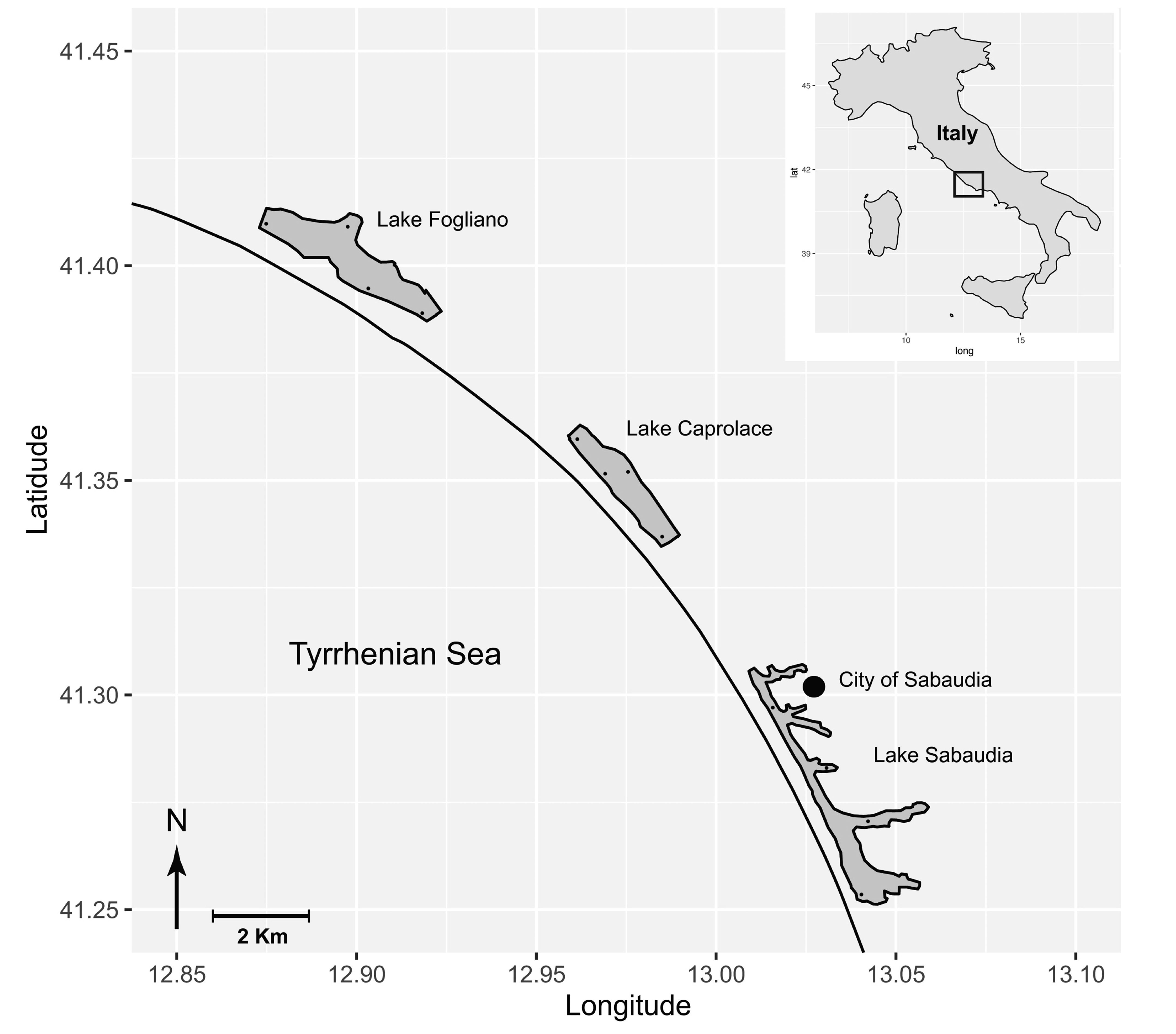
2.1. Study Area

The samplings were carried out in three neighbouring Mediterranean brackish costal lakes located on the Tyrrhenian coast of central Italy (42°28′00″ North–12°51′00″ East): Lake Caprolace, Lake Fogliano and Lake Sabaudia (Figure 1). The three lakes respectively have a surface area of about 3 km², 4 km² and 3.9 km², and mean depths of 3 m, 2 m and 10 m. They are classified as non-tidal lagoons with a maximum tidal excursion of 0.21–0.23 m [44,45,46]. Salinity generally varies between 33.7 and 38.1 PSU in Caprolace, 29.9 and 39.2 PSU in Fogliano, and 28.8 and 33.7 PSU in Sabaudia. The annual average was 36.3 ± 0.8 PSU in Caprolace, 35.3 ± 0.8 PSU in Fogliano and 31.7 ± 0.9 PSU in Sabaudia in 2006–2010 [44]. Data are expressed as mean ± standard error.

The lakes are affected by various forms of anthropogenic disturbance related to organic and inorganic nitrogen inputs from urban treated sewage, livestock farming and agricultural activities, which are widespread in the surrounding areas [2,3].

On average, the mean concentration of total nitrogen was 383.6 ± 23.21 μg/L in Caprolace, 662.6 ± 66.70 μg/L in Fogliano and 1006.1 ± 49.97 μg/L in Sabaudia in 2006–2010. Santoro et al. [2] found the same trend in nitrate concentrations, with 12.2 ± 2.9 μg/L, 42.4 ± 61.3 μg/L and 91.9 ± 70.24 μg/L in Caprolace, Fogliano and Sabaudia respectively in the same period.

Lake Caprolace and Lake Fogliano (hereafter respectively LP and IP), characterised respectively by low and intermediate levels of eutrophication [3,47], are Sites of Community Importance (SCIs) located within the Circeo National Park (Lazio).

Lake Caprolace does not receive water inputs from the hinterland, while Lake Fogliano is affected by nutrient inputs from both the River Rio Martino and the livestock breeding activities practised in the surrounding areas. The annual concentration of Chlorophyll a was generally lower in Caprolace (2.1 ± 0.4 μg/L) than Fogliano (5.8 ± 1.2 μg/L) in 2006–2010.

Lake Sabaudia, the southernmost lake (hereafter HP), is affected by the highest anthropogenic pressure [3], mainly due to runoff from both the city of Sabaudia and cultivated fields in the surrounding areas as well as fishing and mussel farming. In this lake, freshwater inputs are present throughout the year.

Annual algal biomass and Chlorophyll a concentrations in this lake vary from 10.2 to 40.9 μg/L, with an average recorded value in 2006-2010 of 24.2 ± 6.15 μg/L. Further details regarding the study area can be found in Santoro et al. [2] and Jona-Lasinio et al. [3].

2.2. Field Collections

Samples of basal resources (primary producers and detritus), invertebrates and fish were collected in 4 sites per lake between April and May 2012, when primary productivity and invertebrate abundances were high. The sampling sites within each lake were selected from areas with heterogeneous physical and biotic characteristics and a range of anthropogenic impacts deriving from the surrounding areas [2,3]. The sampling sites were located at the northern and southern ends of each lake, and both on the landward and seaward sides (see also Santoro et al. [2]). Macrophytes, algae, and detritus samples were collected by hand and invertebrates by Van Veen grab (volume: 3.5 L) in three replicates per sampling site. The dominant macrophytes were Ruppia sp. and Cymodocea nodosa (Ucria) Ascherson, while the macroalgae were represented by taxa of the genera Chetomorpha, Chondria, Gracilaria, Rytiphloea and Ulva. The detritus was mostly composed of fragments of dead leaves delicately scraped to remove any epibionts and rinsed in distilled water. Phytoplankton samples were collected using a plankton net (20-μm mesh size) and concentrated by centrifugation (2000 rpm for 20 min).

Samples of fish were collected once a day for 3 days in each site. In order to collect pelagic, benthic, resident and migratory fish species, fish samples were collected using fixed weirs and fishing traps placed on the bottom. The fishing traps, made of very fine mesh (0.5 cm), were 1.5 m in diameter at the mouth and were composed of four consecutive chambers of decreasing diameter with a total length of 3.6 m. In addition to A. anguilla and D. annularis, the sampled fish community included the sand smelt Atherina boyeri (Risso, 1810), black goby Gobius niger (Linnaeus, 1758) and the mullets Chelon ramada (Risso, 1827), C. aurata (Risso, 1810), C. saliens (Risso, 1810) and C. labrosus (Risso, 1827), which are known to be prey species of A. anguilla and D. annularis [19,24,25,42,43]. Further fish samples included species belonging to the Sparidae, Scorpaenidae, Clupeidae, Cyprinodontidae, Blenniidae and Belonidae, Gobiidae, Labridae, Moronidae, Mugilidae, Soleidae and Syngnathidae families. Standard length measured in centimetres was recorded for each fish specimen. For each fish species, individuals of different sizes were collected in order to reduce the effects of size variability on isotopic signals. From the sampled fish specimens, including A. anguilla and D. annularis, samples of dorsal white muscle were taken. This tissue provides a long-term (several months) integrated indicator of food sources due to its slow turnover with respect to other tissues (e.g., liver and blood) [32].

After collection, all samples were transported to the laboratory, where specimens were sorted, counted, and identified to the lowest possible taxonomic level and processed for the stable isotope analysis.

2.3. Stable Isotope Analysis (SIA)

Samples were individually stored at −80 °C and freeze-dried for 24 h. Fish specimens were considered individually for isotopic analysis. Muscle samples were also taken from large invertebrates such as crustaceans, for which the tissue was taken from the claws, and bivalves and sea snails, whose tissue was taken from the feet [7]. When present, shells, valves and other exoskeletal parts of animals were removed under dissection microscopes in order to avoid tissue acidification before the stable isotope analysis. For small invertebrates (such as amphipods and polychaetes), the whole body was used. Samples were individually analysed. Plankton biomass was analysed as a whole due to the difficulty of obtaining sufficient biomass for isotopic analysis.

Before the stable isotope analysis, each sample was homogenised to a fine powder using a ball mill (Mini-Mill Fritsch Pulverisette 23: Fritsch Instruments, Idar-Oberstein, Germany). When necessary, samples were pre-acidified using 1M HCl according to the drop-by-drop method [48] in order to eliminate inorganic carbon and re-dried (60 °C) for 72 h to remove the remaining moisture. δ¹⁵N signatures were measured in un-acidified powders to prevent acidification from interfering with the nitrogen analysis [30,49].

Aliquots of 0.25 ± 0.10 mg for the animals and 2.00 ± 0.10 mg for basal resources were placed into tin capsules for C and N stable isotopic analysis (SIA). Each sample was analysed in two replicates. The analyses were carried out using a continuous flow mass spectrometer (IsoPrime100, Isoprime Ltd., Cheadle Hulme, United Kingdom) coupled with an elemental analyser (Elementar Vario Micro-Cube, Elementar Analysensysteme GmbH, Germany).

The isotopic signatures of each sample were expressed in δ units (δ¹⁵N; δ¹³C) as parts per thousand (‰) deviations from international standards (atmospheric N₂ for N; PD-belemnite (PDB) carbonate for C), in accordance with the formula:

δX (‰) = [(Rsample − Rstandard)/Rstandard] × 10³ [50], where X is ¹³C or ¹⁵N and R is the corresponding ratio of heavy to light isotope for the element (¹³C/¹²C or ¹⁵N/¹⁴N). Outputs were standardised with the internal laboratory standard Caffeine IAEA-600 (C₈H₁₀N₄O₂). Measurement errors were found to be typically smaller than 0.05‰.

2.4. Data Analysis

Differences between lakes in terms of animal community composition (considering both fish and benthic invertebrates) were tested using contingency tables based on chi-square (χ²) tests, Monte Carlo permutation tests and the associated Cramer’s V index (a measure of the strength of association among communities; Past 3.0 software package). Specimens collected in each sampling site (and replicates) were grouped by type or taxon (respectively for basal resources and animals) for each lake.

The Shannon diversity index (Hs) of invertebrate fauna for each lake was calculated at family level considering a total abundance of the taxa collected in each lake. Given that assessing Shannon diversity is only possible at the level of equal identification of all taxa, the few individuals belonging to the Gastropoda, Oligochaeta, Nematoda, and Nemertea classes (together accounting for less than 1.5% of total fauna) were excluded from the Shannon diversity index computation. Hutcheson’s diversity t-test and the associated bootstrap procedure (9999 replicates), both available in the Past 3.0 software package, were applied to Hs values to test for significant differences [51]. Hutcheson’s diversity t-test is a modified version of the classic t-test and is based on comparison of Hs variances. The t statistics of Hutcheson are defined as:

$$t=\frac{\left|H{s}_i-H{s}_j\right|}{\sqrt{var\left(H{s}_i\right)+var\left(H{s}_j\right)}}$$

(1)

which follows Student’s t distribution. In the equation, i and j referred to the invertebrate communities of the lakes in paired comparisons, Hs represents the Shannon diversity index and var(Hs) its variance.

The isotopic values of collected organisms were used to reconstruct the diets of the eel Anguilla anguilla and the annular seabream Diplodus annularis in each lake. The diets were estimated on the basis of the Isotopic Trophic Unit (ITU) method [31]. The isotopic signatures of single basal resources, invertebrates, and fish were represented in the bi-dimensional isotopic space (Figure S1). This was subdivided into squares (ITUs) corresponding to 1 × 1‰ δ¹⁵N and δ¹³C values, starting from the lowest δ¹³C value in the dataset and a δ¹⁵N value of zero. The ITUs were thus identified and labelled (Figure S1).

The diets of each ITU containing individuals of the two fish species were calculated by means of Bayesian Mixing Models (R software ver. 3.5.3, SIMMr package) [52] considering a Trophic Enrichment factor (TEF) of 3.4 ± 1.0‰ for δ¹⁵N and 1.0 ± 0.5‰ for δ¹³C [18,37,49,53,54,55,56] and uninformative priors. These TEF values (expressed as mean ± standard deviation) are considered a robust and widely applicable assumption in the presence of multiple trophic pathways and different types of food sources [37,56]. For all SIMMr models, we ran three Markov Chain Monte Carlo chains of 300,000 iterations each with a burn-in of 200,000 and a thinning rate of 100 iterations. We assumed that all incoming food items had the same probability of being included in the consumer’s diet. The model considers both variance in the isotopic signatures of the resources and uncertainty regarding the trophic enrichment of the consumer (TEF). The model results were expressed in the form of a probability distribution of plausible contribution values. The central tendency values of the distribution (mode, mean, median) allowed us to identify the most important food sources, while the upper and lower limits of the credibility ranges (CI: 50%, 75%, 95%) revealed the range of feasible contributions. The pool of food sources was selected based on the mixing model outputs in accordance with Rossi et al. [31]. Since the A. anguilla and D. annularis diet was obtained by starting from the foraging choice of each individual, the overall contribution of some food sources, important at individual level (>5%), could be relatively small (<5%) if considered at the population level (see also [31]). In order to obtain detailed information on the diet of the eel and the seabream these contributions were also considered.

Individuals other than A. anguilla and D. annularis, including basal resources and invertebrates, were excluded from ITU-consumers (but not from potential ITU food sources) before performing the Bayesian mixing models. This was done in order to correctly estimate the diet of A. anguilla and D. annularis. The set of potential ITU food sources was considered on the entire δ¹³C axis and within a given range on the δ¹⁵N axis, i.e., within ±3.4‰ (the TEF) of the value of the consumer [31]. The Bray–Curtis similarity index (BC), based on the contribution of each resource to the diet of the two fish, was also calculated in order to quantify the diet similarity among lakes [36,56]. BC is expressed as proportional similarity ranging from 0, when no common food sources are found for the compared groups, to 1, when the compared groups have the same food sources in the same proportions [36,56].

The symmetric overlap in resource use [57,58,59] was measured in accordance with the Pianka equation [59]:

$$O_{jk}=\frac{{{\displaystyle \sum }}_{i=1}^n{p}_{ij}{p}_{ik}}{\sqrt{{{\displaystyle \sum }}_{i=1}^n{\left(p_{ij}\right)}^2{{\displaystyle \sum }}_{i=1}^n{\left(p_{ik}\right)}^2}}$$

(2)

where the Pianka index (O_jk) represents a symmetric measure of overlap between species j and k, and p_ij and p_ik are the proportional contributions of any given resource i used by species j and species k. The Pianka index ranges from 0 (overlap absent) to 1 (complete overlap).

Chesson’s selectivity index [60] was calculated for each food item to determine possible preferences for particular food sources among those offered:

$${\mathsf{\alpha }}_i=\frac{r_i/n_i}{{{\displaystyle \sum }}_{i=1}^m\left(r_i/n_i\right)}$$

(3)

where α_i is Chesson’s selectivity index, m is the number of food source types, r_i is the proportion of food type i in the diet and n_i is the proportion of food type i in the environment. The value of α_i ranges from 0 to 1, with 0 indicating complete avoidance, values above 1/m indicating preference and 1 indicating absolute preference [61]. Since consumer isotopic ratios provide an integrated measure of prey assimilated over time, we hypothesized that the composition of the taxon in each lake did not vary considerably over the course of a season. Therefore, the Chesson index based on the relationship between assimilated prey and its abundance in the environment could measure the selectivity of food products with a good approximation.

χ² tests were performed to test for differences between lakes in terms of the relative abundance of fauna and differences between food sources in terms of their proportional contribution to the diet of the fish population in each lake. Although it is not possible to establish a theoretical expected value, a χ² test was performed to test for possible differences between IP and LP and between HP and LP, considering the least polluted lake as the reference value.

Differences between lakes in both the δ¹⁵N and δ¹³C isotopic signatures of basal resources and fauna were tested by one-way ANOVA for comparisons between normal distributions (Shapiro–Wilk normality test, p > 0.05) while the Mann–Whitney with Bonferroni correction in cases of multiple comparisons and Kruskal–Wallis tests were used if non-normality was observed (Shapiro–Wilk normality test, p-value < 0.05). Levene’s test for variances was used to test for differences within and between lakes in the δ¹³C variance of primary producers. Kruskal–Wallis tests and associated Mann–Whitney pairwise comparisons were also used to compare the proportional contribution of food items to the diet of A. anguilla and D. annularis.

The niche metrics for both species in each lake were also calculated [62,63,64]. These metrics, originally proposed by Layman et al. [62] for application at community level, can be used at population level to obtain information about trophic diversity within a single population [35,63,64]. These included the ranges (highest to lowest) of δ¹³C (Carbon Range, CR) and δ¹⁵N (Nitrogen Range, NR) values. CR provides information about the variety of food sources exploited by the population (i.e., its trophic generalism), while NR indicates the number of trophic levels (i.e., degree of omnivory) of the population. The isotopic niche widths of both A. Anguilla and D. annularis were calculated as SEAc (Standard Ellipse Area corrected by degree of freedom) using R software ver. 3.5.3, SIBER analysis package [64,65]. The SEAc encompasses the core (about 40%) of the population’s isotopic observations. This is a solid metric for comparing the isotopic niche of populations regardless of sample size and any isotopic outliers in the data [62,64]. Linkage density (L/S) was measured as the average number of feeding links (L) per ITU (S). Finally, based on the proportional contribution of each food source, the trophic niche width (TNW) of each population was measured as the diversity of resources consumed (Hs) by each population and compared among lakes. If not specified otherwise, the results are reported as mean ± standard error (s.e.).

3. Results

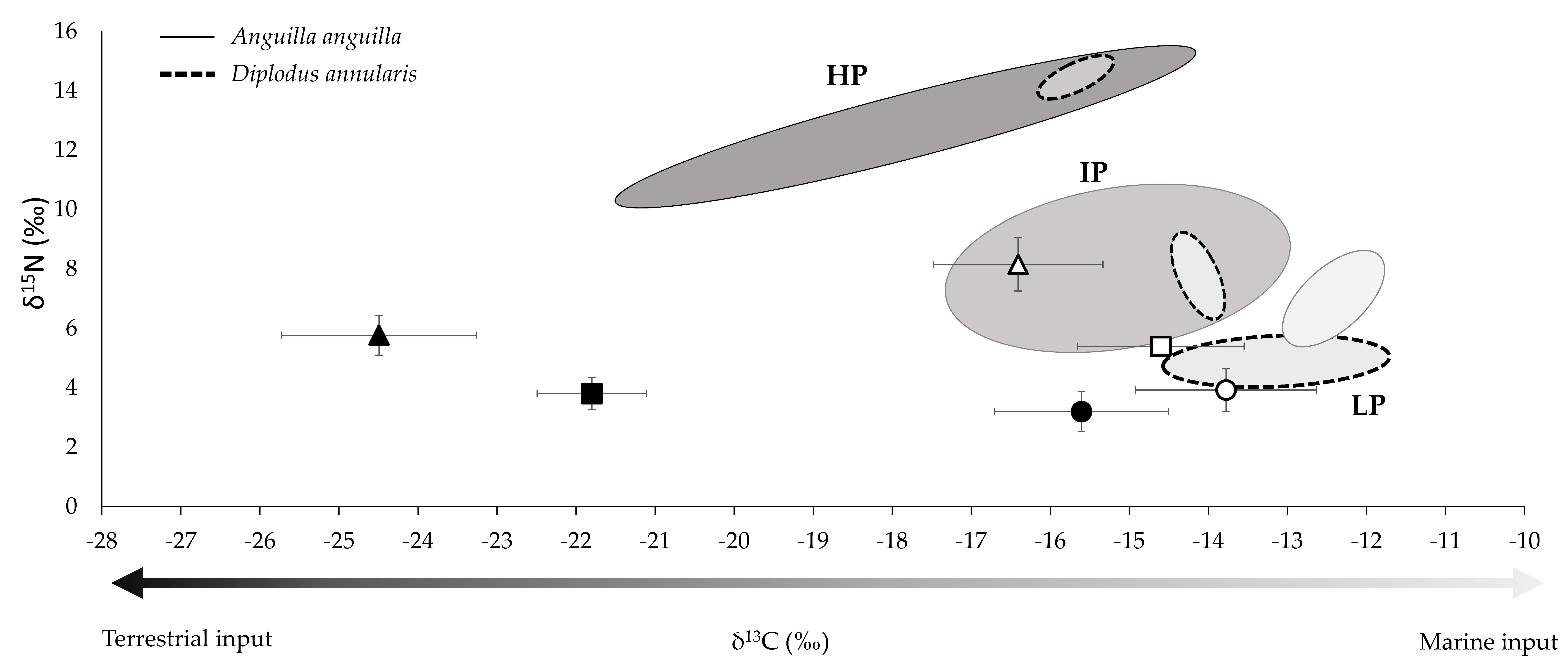
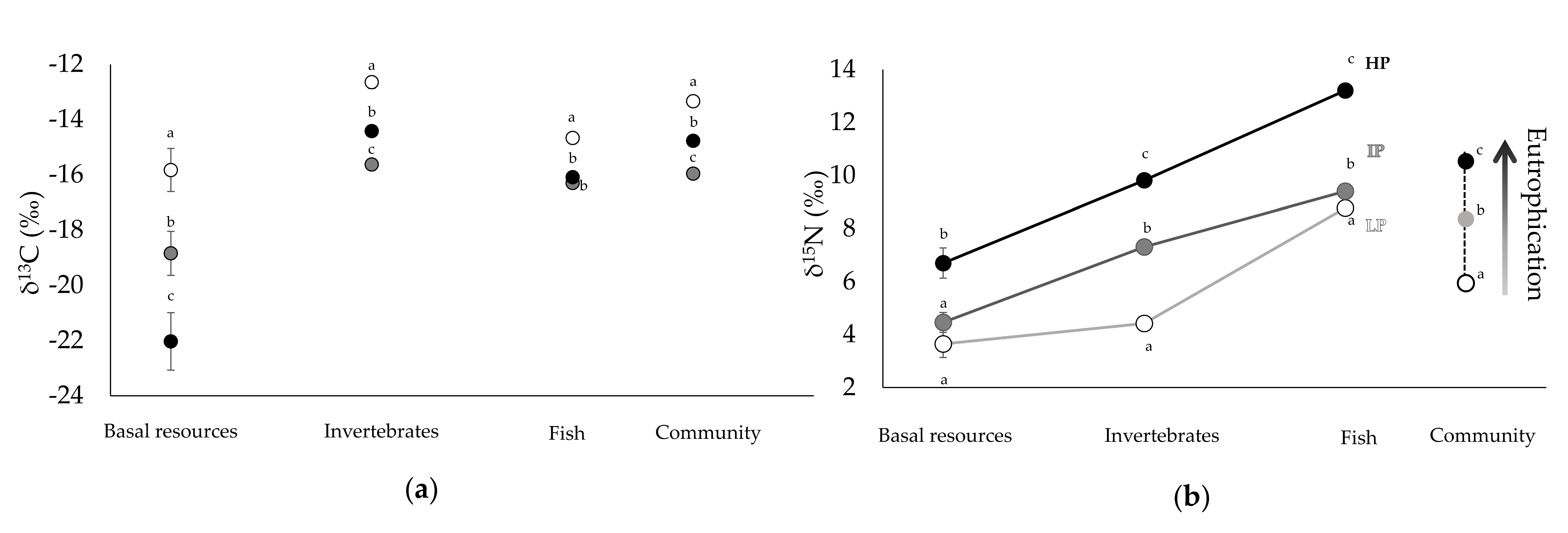
3.1. Community Composition and Isotopic Signatures

A total of 8752 samples comprising basal resources, invertebrates and fish were collected from the three lakes, 8645 (148 taxa) of which were invertebrates and fish (

Table 1. Parameters describing the communities in each Lake. LP, IP and HP: low, intermediate and high eutrophication. N° indicates the sample size. Numbers in parentheses indicate the number of samples analysed. Community indicates both fish and benthic invertebrates. Stable isotopes of δ¹³C and δ¹⁵N are reported as mean (‰) ± s.e. For each parameter, different superscript letters (a,b,c) indicate differences between lakes (one-way ANOVA or Mann–Whitney test; p < 0.05).

	LP	IP	HP
N°
Community	2942 (417)	2777 (502)	2926 (340)
Basal resources	28 (28)	51 (51)	28 (28)
Invertebrates	2793 (268) a	2526 (251) b	2848 (262) a
Fish	149 (145) a	251 (251) b	78 (78) c
δ13C (‰)
Community	−13.34 ± 0.17 a	−15.96 ± 0.13 b	−14.77 ± 0.15 c
Basal resources	−15.83 ± 0.78 a	−18.84 ± 0.80 b	−22.03 ± 1.04 c
Invertebrates	−12.65 ± 0.22 a	−15.63 ± 0.19 b	−14.42 ± 0.18 c
Fish	−14.67 ± 0.21 a	−16.30 ± 0.17 b	−16.09 ± 0.15 b
δ15N (‰)
Community	5.94 ± 0.16 a	8.36 ± 0.14 b	10.54 ± 0.14 c
Basal resources	3.65 ± 0.51 a	4.46 ± 0.38 a	6.70 ± 0.57 b
Invertebrates	4.42 ± 0.16 a	7.31 ± 0.21 b	9.82 ± 0.14 c
Fish	8.79 ± 0.17 a	9.41 ± 0.15 b	13.21 ± 0.16 c

, Table S1).

Malacostraca (Amphipoda, Decapoda and Isopoda), Gastropoda, Anthozoa, Bivalvia, Polychaeta and Ophiuroidea together made up 93.09 ± 3.86 % of invertebrates.

Invertebrate abundance was lower in IP than the other two lakes (Table 1, paired-χ² test, χ² at least 20.46, p-value always <0.0001, Table S2). The composition of both the invertebrate and fish community also varied (contingency table, χ² at least 170.2, p always <0.001, Cramer’s V at least 0.46, Tables S2 and S3). The abundance of some taxa, such as Decapoda and Anthozoa, decreased, while that of others (such as Amphipoda) increased with the pollution level of the lake (paired-χ² test, χ² at least 48.36, p-value always <0.0001). The number of fish taxa varied, i.e., 23 in LP, 17 in IP and 7 in HP. The relative abundance of fish differed between lakes (paired-χ² test, χ² at least 34.21 p-value always <0.0001) and was lowest in HP. The standard length of Anguilla anguilla was lower in HP (35.10 ± 3.63 cm) than the other two lakes (48.81 ± 6.07 cm in LP, 47.66 ± 2.12 cm in IP) (Mann–Whitney test with Bonferroni correction in cases of multiple comparisons, U = 13.0, p-value always <0.05). Similarly, Diplodus annularis had an average standard length of 6.25 ± 0.14 cm in HP, which was lower than LP (8.76 ± 0.31 cm) and IP (9.43 ± 0.41 cm) (Mann–Whitney test with Bonferroni correction in cases of multiple comparisons, U = 2.0, p-value <0.05).

Among the basal resources, detritus showed depleted δ¹³C values, while primary producers were δ¹³C-enriched (Figure 2). δ¹³C-enrichment was also observed in pelagic fish with specialist diets such as Atherina boyeri (δ¹³C = −15.34 ± 0.08‰ in LP, −17.45 ± 1.35‰ in IP and −16.14 ± 0.90‰ in HP). Since neither the mean nor the variance (σ²) of δ¹³C in the primary producers differed significantly either within each lake or between lakes (one-way ANOVA and associated Levene’s test for homogeneity of variances, F at least 0.1412, p-value always >0.05), we concluded that the presence of a salinity gradient within a lake could not have an effect on the isotopic variability of the baseline. δ¹⁵N values of primary producers increased with eutrophication (one-way ANOVA, F: 5.80, p <0.01).

The isotopic differences observed in basal resources reflected those observed in the whole community (Table 1, Figure 3; Kruskal–Wallis, Hc at least 127.1, p-value < 0.001; for δ¹³C Mann–Whitney with Bonferroni correction for multiple comparisons, U at least 45,590, p-value always <0.001 and for δ¹⁵N Mann–Whitney, U at least 421.57 with Bonferroni correction for multiple comparisons, p-value always <0.001, Figure 3) and in A. anguilla and D. annularis.

The δ¹³C and δ¹⁵N isotopic signatures of Anguilla anguilla and Diplodus annularis differed between lakes (Kruskal–Wallis, Hc at least 35.5, p-value <0.001). δ¹³C values were higher in the least polluted lake (

Table 2. Isotopic niche and food web metrics of the eel Anguilla anguilla and the seabream Diplodus annularis in each lake. LP: low, IP: intermediate, HP: high eutrophication. N: sample size, ITUs: Isotopic Trophic Units, δ¹³C (‰) and δ¹⁵N (‰) (mean ± s.e.), CR: Carbon Range, NR: Nitrogen Range, L: number of feeding links, S: number of ITUs in the diet, L/S: Linkage density, SEAc: Standard Ellipse Area “corrected” (SEAc) by degree of freedom, TNW: Trophic Niche Width. For details of metrics, please refer to the materials and methods section. For each parameter, different superscript letters (a,b,c) indicate differences between lakes (Mann–Whitney test with Bonferroni correction for multiple comparisons; p-value <0.05).

	Anguilla anguilla			Diplodus annularis
	LP	IP	HP	LP	IP	HP
N	8	16	10	8	6	8
ITUs
δ13C (‰)	−12.76 ± 0.11 a	−15.07 ± 0.15 b	−16.31 ± 0.16 c	−13.49 ± 0.16 a	−16.23 ± 0.14 a	−15.34 ± 0.19 b
δ15N (‰)	8.27 ± 0.19 a	9.62 ± 0.12 a	13.58 ± 0.11 b	5.81 ± 0.15 a	7.99 ± 0.14 b	10.24 ± 0.15 c
CR	2.05	9.52	6.19	2.17	0.35	0.65
NR	3.15	5.79	3.51	0.67	0.96	0.74
Taxa
δ13C (‰)	−12.29 ± 0.19 a	−15.01 ± 0.53 b	−17.20 ± 1.12 c	−13.00 ± 0.49 a	−14.00 ± 0.10 a	−15.57 ± 0.16 b
δ15N (‰)	9.08 ± 0.32 a	9.50 ± 0.36 a	12.96 ± 0.51 b	7.73 ± 0.17 a	9.59 ± 0.29 b	13.87 ± 0.16 c
CR	1.55	4.66	6.19	2.17	0.35	0.65
NR	2.54	2.59	2.86	0.67	0.96	0.74
L	30	84	33	28	13	14
S	19	42	22	21	10	11
L/S	1.6	2.0	1.5	1.3	1.3	1.3
SEAc	1.46	9.62	4.84	1.55	0.45	0.32
TNW	1.81	2.06	2.32	2.15	2.28	1.98

; Mann–Whitney with Bonferroni correction for multiple comparisons, U at least 3392.5, p-value always <0.001), while δ¹⁵N values increased with eutrophication (Table 2; Mann–Whitney with Bonferroni correction for multiple comparisons, U at least 555, p-value always <0.001).

Specifically, in A. anguilla, the more generalist of the two species, δ¹³C values reflected the shift of inputs from marine to terrestrial origin passing from the least to the most eutrophic lake (Figure 2 and Table 1 and Table 2).

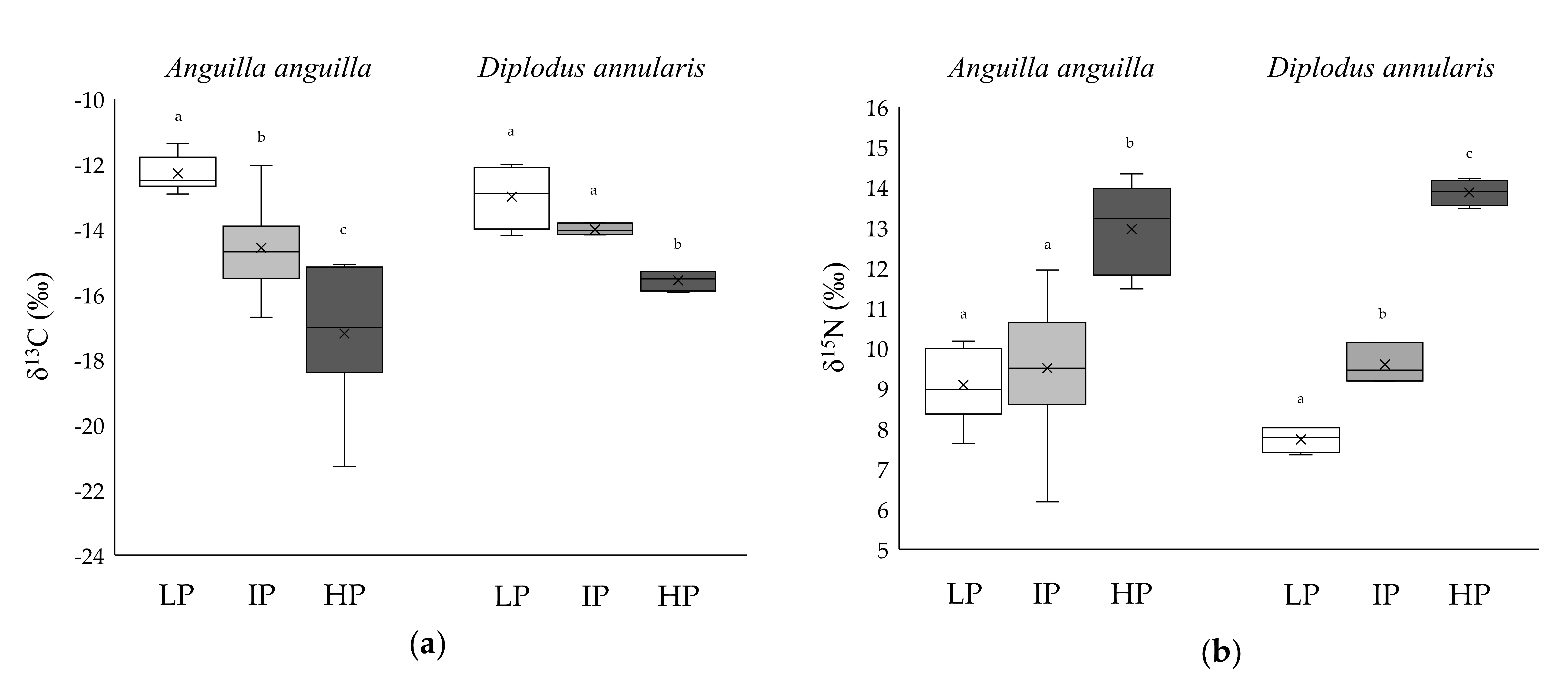
3.2. Niche Metrics and Diet of Anguilla anguilla

The isotopic signatures and niche metrics of Anguilla anguilla varied among lakes (Table 2, Figure 2, Figure 3 and Figure 4; Kruskal–Wallis, Hc least 12.06, p-value <0.001). The highest δ¹⁵N values were observed in HP (Table 2; Mann–Whitney with Bonferroni correction in cases of multiple comparisons, U at least 0.1, p-value always <0.001). The Carbon Range increased with eutrophication (Figure 4, Table 2) and the largest Nitrogen Range was observed in the eutrophic lake (Table 2).

Overall, no correlation between the body length and δ¹³C (‰) of Anguilla anguilla was observed in any lake (Pearson correlation, p >0.05).

Anguilla anguilla had 5 ITUs in LP and HP and 12 ITUs in IP, where the eel-resource ITU linkage density was highest (Table 2). ITU-based mixing models showed no differences between lakes in terms of the overall contribution of invertebrates to the eels’ diet (Figure 5a).

By contrast, the consumption of basal resources increased and piscivory decreased with increasing levels of pollution (i.e., from LP to HP;

Table 3. Proportional contribution (in %) of food sources to the diet of A. anguilla in each lake, obtained from ITU-based mixing models. LP: low anthropogenic pressure, IP: intermediate anthropogenic pressure, HP: high anthropogenic pressure. The contribution of each food source is reported as the mean (±s.e.). “Taxa” indicates the number of taxa belonging to the respective group in the diet of A. anguilla. The overall contribution of basal resources, invertebrates and fish is reported as the mean (%) ± s.e. Different superscript letters (a,b,c) indicate differences between lakes in the contribution of categories of food sources to the diet (χ²-test, p-value <0.05). For details please refer to the methods section.

	LP		IP		HP
Food Sources	Taxa	Contribution	Taxa	Contribution	Taxa	Contribution
TELEOSTS
Actinopterygii	7	34.76 ± 1.90	12	30.65 ± 0.50	3	12.18 ± 1.50
CNIDARIANS
Anthozoa	2	4.40 ± 0.60	4	3.17 ± 0.10	2	3.39 ± 0.20
Hydrozoa	-	-	-	-	1	1.67 ± 0.10
ASCIDIANS
Ascidiacea	-	-	-	-	1	1.82 ± 0.10
BASAL RESOURCES
Algae	1	0.75 ± 0.10	-	-	1	1.55 ± 0.10
Detritus	2	1.81 ± 0.40	4	5.33 ± 0.60	2	9.03 ± 0.50
Phytoplankton	-	-	1	0.42 ± 0.10	1	3.10 ± 0.10
Aquatic plants	1	0.75 ± 0.10	4	4.68 ± 0.40	1	4.19 ± 0.10
MOLLUSCS
Bivalvia	1	0.43 ± 0.10	4	5.68 ± 0.40	4	10.35 ± 0.90
Gastropoda	8	13.06 ± 0.40	3	1.57 ± 0.20	2	2.95 ± 1.00
ANELLIDA
Clitellata (Oligochaeta)	-	-	-	-	1	2.60 ± 0.10
Polychaeta	6	5.62 ± 0.20	5	6.99 ± 0.20	13	30.41 ± 0.60
ECHINODERMS
Eleutherozoa (Asteroidea)	1	0.29 ± 0.10	-	-	-	-
Euechinoidea (Echinoidea)	1	4.40 ± 0.10	-	-	-	-
Ophiuroidea	-	-	1	2.01 ± 0.10	-	-
ARTHROPODS
Insecta	-	-	1	1.42 ± 0.10	1	1.62 ± 0.10
Malacostraca
Amphipoda	4	4.74 ± 0.30	4	5.10 ± 0.40	2	4.13 ± 0.50
Decapoda	4	27.84 ± 4.60	7	26.13 ± 1.90	2	9.11 ± 1.90
Isopoda	2	1.15 ± 1.70	4	5.78 ± 0.30	-	-
NEMERTEANS
Nemertea	-	-	1	1.08 ± 0.10	1	1.91 ± 0.10
BASAL RESOURCES		3.31 ± 0.35 a		10.43 ± 1.54 ab		17.87 ± 1.60 b
INVERTEBRATES		61.93 ± 2.92		58.93 ± 2.15		69.96 ± 2.56
FISH		34.76 ± 1.90 a		30.65 ± 0.50 a		16.18 ± 1.50 b

Figure 5a).

A. anguilla showed a generalist diet including 20 different categories of food source (Table 3, Figure 6 and Figure 7). Some of these were common to the three lake populations (e.g., Actinopterygii, Bivalvia, Gastropoda, Decapoda and Polychaeta) but their consumption varied. The Bray–Curtis index (BC) applied to diet showed a lower similarity between the HP population and the others (76% similarity between LP and IP vs. 41% between LP and HP, and 54% between IP and HP). Specifically, in LP the diet of A. anguilla was mostly based on Actinopterygii (34.76% ± 1.90), Decapoda (27.84% ± 4.60) and Gastropoda (13.06% ± 0.40), in IP on Actinopterygii (30.65% ± 0.50) and Decapoda (26.13% ± 1.90) and in HP on Polychaeta (30.41% ± 0.60), Actinopterygii (12.18% ± 1.50), Bivalvia (10.35% ± 0.90), detritus (9.03% ± 0.50) and Decapoda (9.11% ± 1.90) (Table 3, Figure 6).

The difference in resource use was associated with a difference in trophic niche width (Figure 2, Figure 3, Figure 4, Figure 5 and Figure 6), which increased with eutrophication (TNW: 1.81, 2.06 and 2.32 in LP, IP and HP respectively), with significant differences between HP and LP (bootstrap comparison among populations, p <0.0001).

3.3. Niche Metrics and Diet of Diplodus annularis

The δ¹³C and δ¹⁵N of Diplodus annularis varied across lakes (Figure 2, Figure 3 and Figure 4, Kruskal–Wallis for both δ¹³C and δ¹⁵N, Hc at least 35.5, p-value <0.001). In addition, no significant correlation between the body length and δ¹³C (‰) of Diplodus annularis was observed in any lake (Pearson correlation, p >0.05).

δ¹⁵N increased with the level of pollution (Table 2, Figure 4). The Carbon Range was highest in LP while no differences in Nitrogen Range were observed between lakes (Table 2). The seabreams had four ITUs in LP and two ITUs in both IP and HP (Table 2). No differences in the linkage density (L/S) of the ITUs or in SEAc were observed between lakes (Table 2).

Mixing models based on the single ITU values showed similar average contributions of basal resources, invertebrates and fish in the lakes (Figure 5b; paired-χ² test, p-value always >0.05).

However, when taxa in each category were distinguished, diet similarity between LP and HP was 55%, while between IP and both LP and HP it was 61% (Bray–Curtis index, BC).

Overall, the diet of D. annularis was based on 17 different taxa, and invertebrates represented more than 70% of it in all lakes (

Table 4. Diet composition of Diplodus annularis in each lake. Proportional contribution (in %) of food sources to the diet of D. annularis obtained from ITU-based mixing models. LP: low anthropogenic pressure, IP: intermediate anthropogenic pressure, HP: high anthropogenic pressure. The contribution of each food source is reported as the mean (± s.e.). “Taxa” indicates the number of taxa belonging to the respective group in the diet of D. annularis. The overall contribution of basal resources, invertebrates and fish is reported as the mean (%) ± s.e.

	LP		IP		HP
Food Sources	Taxa	Contribution	Taxa	Contribution	Taxa	Contribution
TELEOSTS
Actinopterygii	4	12.69 ± 0.49	5	10.84 ± 0.28	3	18.56 ± 0.78
CNIDARIANS
Anthozoa	2	10.21 ± 1.31	3	5.15 ± 0.69	1	1.28 ± 4.75
Hydrozoa	-	-	-	-	-	-
BASAL RESOURCES
Algae	1	2.01 ± 0.10	-	-	-	-
Detritus	1	1.56 ± 0.58	2	5.91 ± 0.29	1	3.02 ± 5.00
Phytoplankton	-	-	-	-	-	-
Aquatic plants	2	2.88 ± 0.91	4	8.07 ± 0.10	1	5.05 ± 0.28
MOLLUSCS
Bivalvia	-	-	2	6.24 ± 0.76	2	3.37 ± 0.44
Gastropoda	6	20.65 ± 1.06	1	1.08 ± 5.00	2	4.29 ± 1.23
ANELLIDS
Clitellata (Oligochaeta)	-	-	-	-	1	2.73 ± 5.00
Polychaeta	8	9.71 ± 0.55	3	10.89 ± 0.69	8	34.76 ± 1.12
ECHINODERMS
Eleutherozoa (Asteroidea)	1	0.99 ± 5.00	-	-	-	-
Euechinoidea (Echinoidea)	1	6.04 ± 5.00	-	-	-	-
Ophiuroidea	-	-	1	3.54 ± 0.75	-	-
ARTHROPODS
Insecta	-	-	1	3.1 ± 1.06	1	0.87 ± 5.00
Malacostraca
Amphipoda	3	8.43 ± 1.13	3	9.86 ± 1.54	2	7.8 ± 1.10
Decapoda	5	22.03 ± 1.37	5	27.86 ± 1.69	2	14.67 ± 1.03
Isopoda	3	2.8 ± 0.31	4	4.85 ± 0.20	-	-
NEMERTEANS
Nemertea	-	-	1	2.61 ± 0.71	1	3.6 ± 0.74
BASAL RESOURCES		6.45 ± 0.39		13.98 ± 1.08		8.07 ± 1.02
INVERTEBRATES		80.86 ± 2.7		75.18 ± 2.46		73.37 ± 3.61
FISH		12.68 ± 0.49		10.82 ± 0.28		18.57 ± 0.78

, Figure 5 and Figure 6). Among these, Decapoda (22.03% ± 1.37), Gastropoda (20.65% ± 1.06) and Actinopterygii (12.69% ± 0.49) contributed most to the diet of D. annularis in LP (Figure 6); Decapoda (27.86% ± 1.69), Actinopterygii (10.84% ± 0.28) and Amphipoda (9.86% ± 1.54) in IP (Figure 5); and Polychaeta (34.76% ± 1.12), Actinopterygii (18.56% ± 0.78) and Decapoda (14.67% ± 1.03) in HP.

The trophic niche was significantly narrower in HP than LP and IP (Figure 6; TNW: 1.98 vs. 2.15 and 2.28 respectively; bootstrap comparison among populations, p <0.05). The niche overlap between D. annularis and A. anguilla decreased from the eutrophic to the unpolluted lake (O = 0.95, 0.87 and 0.84 in HP, IP and LP respectively).

4. Discussion

Our results indicate that anthropogenic inputs affected the composition and abundance of the lake animal community. Specifically, the diversity of fish decreased, and trophic choices of the eel Anguilla anguilla and the seabream Diplodus annularis changed, with increasing eutrophication. A. anguilla, which was more piscivorous than the seabream at low and intermediate eutrophication, increased its consumption of invertebrates and basal resources. On the other hand, the seabream, which fed more on invertebrates, increased its preference for polychaetes. The high selectivity for polychaetes in the highly eutrophicated lake could be due to the facilitated capture of these preys and their good contribution to the energy supply of their predators compared to other aquatic invertebrates [66,67,68]. Changes in the feeding choices of the two fish species resulted in increased interspecific niche overlap, suggesting that eutrophication may have strong bottom-up effects on interspecific interactions [69,70].

Previous research demonstrates that the δ¹⁵N values of the aquatic biota reflect anthropogenic nitrogen inputs from the surrounding terrestrial areas [7,10,71,72]. In our study, increased eutrophication was associated with higher δ¹⁵N in the fish community, as previously observed by Santoro et al. [2] and Jona-Lasinio et al. [3] for invertebrates and primary producers respectively. Our results indicate that in transitional waters, individual fish δ¹⁵N could be a useful indicator of anthropogenic N transfer along food webs [10,73], while the range of δ¹³C in the fish population could reflect the diversity of C inputs, emphasising the need for ecological monitoring in these productive ecosystems.

The distinct carbon isotopic signatures (δ¹³C) of primary producers (e.g., terrestrial vs. aquatic vegetation) allowed us to discern the origin of the organic matter contributing to the nutrient pool of water bodies [7,33,34,74]. Specifically, depleted δ¹³C organic matter values indicated the contribution to the organic matter pool of allochthonous (terrestrial) carbon, while enriched δ¹³C indicated autochthonous primary production, as also observed in other aquatic ecosystems [7,34,35,74]. Although it was not in the remit of this study to investigate the cause, carbon enrichment was also visible in pelagic and strictly specialist species such as the sand smelt, A. boyeri. In addition, neither the mean nor the variance of δ¹³C of primary producers differed significantly between sites within the same lake or between different lakes. This allowed us to exclude possible interferences in the isotopic baseline arising from environmental parameters such as the salinity and oxygenation levels of the respective area. The larger contribution of terrestrial organic matter in HP may be due to the large input of fresh water that this lake receives from the hinterland, as indicated by the low salinity generally observed in this lake compared to the other two. These results are consistent with what has been observed in similar environments [7,74,75].

Large Carbon Ranges suggest multiple carbon sources at the base of the food web [7,35,62,63,64]. The supply of organic matter from multiple sources in the three lakes was evident in the δ¹³C values of A. anguilla, which shifted from marine to terrestrial input with the increasing pollution. Its larger Carbon Range in the eutrophic lake indicates that this species integrated both autochthonous and allochthonous carbon pathways, while in the unpolluted lake it relied mainly on the autochthonous one.

It is acknowledged that increased N-loads promote significant changes in aquatic productivity [76] that could potentially affect the composition of the prey community [77,78]. This in turn might be reflected in the feeding behaviour of consumers at all trophic levels [2,7,79].

In our study, increased N pollution resulted in altered community composition, with decreasing diversity, which seemed to affect the feeding preference and niche width of Anguilla anguilla and Diplodus annularis. The feeding regime of the two species is known to be characterised by marked generalism and trophic plasticity [19,22,42,43,80]. However, while the eel enlarged its trophic niche, feeding off multiple resources at various trophic levels in eutrophic conditions, the seabream concentrated on a small number of invertebrates. Although dietary changes are known to depend primarily on size and growth stage [81,82,83], in our study neither A. anguilla nor D. annularis showed a relationship between body size and δ¹³C signatures. The greater trophic generalism and omnivory of eels with eutrophication may be due to the different density, accessibility and availability of the prey at higher trophic levels [19,22,24,42,43] as well as to an altered presence of potential competitors for the same food sources [78]. This was also confirmed by the results of the Bayesian mixing models, which showed a shift with eutrophication in the diet of Anguilla anguilla mostly from pelagic (fish) to benthic (invertebrates) prey, regardless of their abundance. Bouchereau et al. [24,25] reported Teleosts, amphipods and decapods as the predominant prey in the diet of A. anguilla in two North-Mediterranean lagoons, and that prey selection could be linked to the activity and accessibility of the prey itself. Rosecchi [42], Pita et al. [23] and Chaouch et al. [19] indicated molluscs (bivalves and gastropods), crustaceans, polychaetes and Teleosts as the main items in the diet of D. annularis in lagoons and coastal waters. Lammens et al. [84] and Dörner et al. [80] identified A. anguilla as belonging to the piscivorous community in many European lakes. In our study, the adoption of piscivory in the least eutrophic lake allowed the eel to reduce niche overlap [80,84,85] and therefore potential competition with other fish.

However, the trophic behaviour of the two species can be expressed differently by individuals within populations [18,20,21], enabling A. anguilla and D. annularis to include several food sources in their diet even in a single area [19,25]. In this context, the individual isotopic characterisations of carbon (δ¹³C) and nitrogen (δ¹⁵N), coupled with diet reconstruction at the isotopic trophic unit level (ITU, as recently proposed by Rossi et al. [31]) were crucial to the detailed estimation of the diets of the two fish species with high trophic generalism and omnivory. This allowed us to consider the possibility that each individual consumer could draw on the whole spectrum of potential food sources available within each lake [31]. In this way, we are able to describe the trophic plasticity and generalism of two ecologically and economic important fish species, and hence the real variation of the diet within the same populations under a range of eutrophication conditions.

5. Concluding Remarks

Understanding the trophic response of the community to eutrophication and depicting the structure of food webs in coastal lakes is still problematic [14], mainly due to the extraordinary biological diversity and complexity of the potential trophic links between species [2,86,87]. In our study, the stable isotope analysis of carbon (δ¹³C) and nitrogen (δ¹⁵N) provided an effective approach with which to (1) track the propagation of anthropogenic nutrient inputs along food chains, (2) evaluate the relative contributions of food sources to fish diets, and (3) quantify the trophic relationships between organisms [31,37,62,87,88,89]. Here, the diet resulting from the application of the method recently proposed by Rossi et al. [31] substantially improved our ability to understand the response of communities to increasing eutrophication, as well as its effect on the feeding behaviour and food choices of important fish species in Mediterranean coastal lakes. Together, our results confirm food web theory as a powerful approach for obtaining valuable information for the management and conservation of these complex and productive ecosystems.

References

1. Basset, A.; Sabetta, L.; Fonnesu, A.; Mouillot, D.; Chi, T.D.; Viaroli, P.; Giordani, G.; Reizopoulou, S.; Abbiati, M.; Carrada, G.C. Typology in Mediterranean transitional waters: New challenges and perspectives. Aquat. Conserv. Mar. Freshw. Ecosyst. 2006, 16, 441–455. [Google Scholar] [CrossRef]
2. Santoro, R.; Bentivoglio, F.; Carlino, P.; Calizza, E.; Costantini, M.L.; Rossi, L. Sensitivity of food webs to nitrogen pollution: A study of three transitional water ecosystems embedded in agricultural landscapes. Transit. Waters Bull. 2014, 8, 84–97. [Google Scholar]
3. Jona-Lasinio, G.; Costantini, M.L.; Calizza, E.; Pollice, A.; Bentivoglio, F.; Orlandi, L.; Careddu, G.; Rossi, L. Stable isotope-based statistical tools as ecological indicator of pollution sources in Mediterranean transitional water ecosystems. Ecol. Indic. 2015, 55, 23–31. [Google Scholar] [CrossRef]
4. Elliott, M.; Whitfield, A.K.; Potter, I.C.; Blaber, S.J.M.; Cyrus, D.P.; Nordlie, F.G.; Harrison, T.D. The guild approach to categorizing estuarine fish assemblages: A global review. Fish Fish. 2007, 8, 241–268. [Google Scholar] [CrossRef]
5. Chapman, P.M. Management of coastal lagoons under climate change. Estuar. Coast. Shelf Sci. 2012, 110, 32–35. [Google Scholar] [CrossRef]
6. Orlandi, L.; Bentivoglio, F.; Carlino, P.; Calizza, E.; Rossi, D.; Costantini, M.L.; Rossi, L. δ15N variation in Ulva lactuca as a proxy for anthropogenic nitrogen inputs in coastal areas of Gulf of Gaeta (Mediterranean Sea). Mar. Pollut. Bull. 2014, 84, 76–82. [Google Scholar] [CrossRef]
7. Careddu, G.; Costantini, M.L.; Calizza, E.; Carlino, P.; Bentivoglio, F.; Orlandi, L.; Rossi, L. Effects of terrestrial input on macrobenthic food webs of coastal sea are detected by stable isotope analysis in Gaeta Gulf. Estuar. Coast. Shelf Sci. 2015, 154, 158–168. [Google Scholar] [CrossRef]
8. Fiorentino, F.; Cicala, D.; Careddu, G.; Calizza, E.; Jona-Lasinio, G.; Rossi, L.; Costantini, M.L. Epilithon δ15N signatures indicate the origins of nitrogen loading and its seasonal dynamics in a volcanic Lake. Ecol. Indic. 2017, 79, 19–27. [Google Scholar] [CrossRef]
9. Howarth, R.W. Coastal nitrogen pollution: A review of sources and trends globally and regionally. Harmful Algae 2008, 8, 14–20. [Google Scholar] [CrossRef]
10. Calizza, E.; Favero, F.; Rossi, D.; Careddu, G.; Fiorentino, F.; Sporta Caputi, S.; Rossi, L.; Costantini, M.L. Isotopic biomonitoring of N pollution in rivers embedded in complex human landscapes. Sci. Total Environ. 2020, 706, 136081. [Google Scholar] [CrossRef]
11. Fox, S.E.; Teichberg, M.; Olsen, Y.S.; Heffner, L.; Valiela, I. Restructuring of benthic communities in eutrophic estuaries: Lower abundance of prey leads to trophic shifts from omnivory to grazing. Mar. Ecol. Prog. Ser. 2009, 380, 43–57. [Google Scholar] [CrossRef] [Green Version]
12. Martínez-Durazo, A.; García-Hernández, J.; Páez-Osuna, F.; Soto-Jiménez, M.F.; Jara-Marini, M.E. The influence of anthropogenic organic matter and nutrient inputs on the food web structure in a coastal lagoon receiving agriculture and shrimp farming effluents. Sci. Total Environ. 2019, 664, 635–646. [Google Scholar] [CrossRef]
13. Calizza, E.; Costantini, M.L.; Rossi, L. Effect of multiple disturbances on food web vulnerability to biodiversity loss in detritus-based systems. Ecosphere 2015, 6, 1–20. [Google Scholar] [CrossRef] [Green Version]
14. Carlier, A.; Riera, P.; Amouroux, J.-M.; Bodiou, J.-Y.; Desmalades, M.; Grémare, A. Food web structure of two Mediterranean lagoons under varying degree of eutrophication. J. Sea Res. 2008, 60, 264–275. [Google Scholar] [CrossRef]
15. Capoccioni, F.; Costa, C.; Canali, E.; Aguzzi, J.; Antonucci, F.; Ragonese, S.; Bianchini, M.L. The potential reproductive contribution of Mediterranean migrating eels to the Anguilla anguilla stock. Sci. Rep. 2014, 4, 1–7. [Google Scholar] [CrossRef] [Green Version]
16. Trojette, M.; Faleh, A.B.; Fatnassi, M.; Marsaoui, B.; Mahouachi, H.; El, N.; Chalh, A.; Quignard, J.P.; Trabelsi, M. Stock discrimination of two insular populations of Diplodus annularis (ACTINOPTERYGII: PERCIFORMES: SPARIDAE) along the coast of Tunisia by analysis of otolith shape. Acta Ichtyologica et Piscicatoria 2015, 45, 363–372. [Google Scholar] [CrossRef] [Green Version]
17. Bilotta, G.S.; Sibley, P.; Hateley, J.; Don, A. The decline of the European eel Anguilla anguilla: Quantifying and managing escapement to support conservation. J. Fish Biol. 2011, 78, 23–38. [Google Scholar] [CrossRef]
18. Harrod, C.; Grey, J.; McCarthy, T.K.; Morrissey, M. Stable isotope analyses provide new insights into ecological plasticity in a mixohaline population of European eel. Oecologia 2005, 144, 673–683. [Google Scholar] [CrossRef]
19. Chaouch, H.; Ben Abdallah-Ben Hadj Hamida, O.; Ghorbel, M.; Jarboui, O. Feeding habits of the annular seabream, Diplodus annularis (Linnaeus, 1758) (Pisces: Sparidae), in the Gulf of Gabes (Central Mediterranean). Cahiers de Biologie Marine 2014, 55, 13–19. [Google Scholar]
20. Vizzini, S.; Mazzola, A. Seasonal variations in the stable carbon and nitrogen isotope ratios (13C/12C and 15N/14N) of primary producers and consumers in a western Mediterranean coastal lagoon. Mar. Biol. 2003, 142, 1009–1018. [Google Scholar] [CrossRef]
21. Persic, A.; Roche, H.; Ramade, F. Stable carbon and nitrogen isotope quantitative structural assessment of dominant species from the Vaccarès Lagoon trophic web (Camargue Biosphere Reserve, France). Estuar. Coast. Shelf Sci. 2004, 60, 261–272. [Google Scholar] [CrossRef]
22. Mariani, S.; Maccaroni, A.; Massa, F.; Rampacci, M.; Tancioni, L. Lack of consistency between the trophic interrelationships of five sparid species in two adjacent central Mediterranean coastal lagoons. J. Fish Biol. 2002, 61, 138–147. [Google Scholar] [CrossRef]
23. Pita, C.; Gamito, S.; Erzini, K. Feeding habits of the gilthead seabream (Sparus aurata) from the Ria Formosa (southern Portugal) as compared to the black seabream (Spondyliosoma cantharus) and the annular seabream (Diplodus annularis). J. Appl. Ichthyol. 2002, 18, 81–86. [Google Scholar] [CrossRef]
24. Bouchereau, J.L.; Marques, C.; Pereira, P.; Guélorget, O.; Lourié, S.M.; Vergne, Y. Feeding behaviour of Anguilla anguilla and trophic resources in the Ingril Lagoon (Mediterranean, France). Cahiers de Biologie Marine 2009, 50, 319. [Google Scholar]
25. Bouchereau, J.L.; Marques, C.; Pereira, P.; Guélorget, O.; Vergne, Y. Food of the European eel Anguilla anguilla in the Mauguio lagoon (Mediterranean, France). Acta Adriat. 2009, 50, 159–170. [Google Scholar]
26. Pasquaud, S.; Elie, P.; Jeantet, C.; Billy, I.; Martinez, P.; Girardin, M. A preliminary investigation of the fish food web in the Gironde estuary, France, using dietary and stable isotope analyses. Estuar. Coast. Shelf Sci. 2008, 78, 267–279. [Google Scholar] [CrossRef]
27. França, S.; Vasconcelos, R.P.; Tanner, S.; Máguas, C.; Costa, M.J.; Cabral, H.N. Assessing food web dynamics and relative importance of organic matter sources for fish species in two Portuguese estuaries: A stable isotope approach. Mar. Environ. Res. 2011, 72, 204–215. [Google Scholar] [CrossRef]
28. Woodward, G.; Hildrew, A.G. Invasion of a stream food web by a new top predator. J. Anim. Ecol. 2001, 70, 273–288. [Google Scholar] [CrossRef]
29. Peterson, B.J.; Fry, B. Stable Isotopes in Ecosystem Studies. Annu. Rev. Ecol. Syst. 1987, 18, 293–320. [Google Scholar] [CrossRef]
30. Kwak, T.J.; Zedler, J.B. Food web analysis of southern California coastal wetlands using multiple stable isotopes. Oecologia 1997, 110, 262–277. [Google Scholar] [CrossRef]
31. Rossi, L.; Sporta Caputi, S.; Calizza, E.; Careddu, G.; Oliverio, M.; Schiaparelli, S.; Costantini, M.L. Antarctic food web architecture under varying dynamics of sea ice cover. Sci. Rep. 2019, 9, 1–13. [Google Scholar] [CrossRef]
32. Fry, B. Stable Isotope Ecology; Springer: New York, NY, USA, 2006; Volume 521. [Google Scholar]
33. Fry, B. Coupled N, C and S stable isotope measurements using a dual-column gas chromatography system. Rapid Commun. Mass Spectrom. 2007, 21, 750–756. [Google Scholar] [CrossRef]
34. Rossi, L.; Costantini, M.L.; Carlino, P.; di Lascio, A.; Rossi, D. Autochthonous and allochthonous plant contributions to coastal benthic detritus deposits: A dual-stable isotope study in a volcanic lake. Aquat. Sci. 2010, 72, 227–236. [Google Scholar] [CrossRef]
35. Careddu, G.; Calizza, E.; Costantini, M.L.; Rossi, L. Isotopic determination of the trophic ecology of a ubiquitous key species—The crab Liocarcinus depurator (Brachyura: Portunidae). Estuar. Coast. Shelf Sci. 2017, 191, 106–114. [Google Scholar] [CrossRef]
36. Calizza, E.; Careddu, G.; Sporta Caputi, S.; Rossi, L.; Costantini, M.L. Time- and depth wise trophic niche shifts in Antarctic benthos. PLoS ONE 2018, 13, e0194796. [Google Scholar] [CrossRef] [Green Version]
37. Post, D.M. Using Stable Isotopes to Estimate Trophic Position: Models, Methods, and Assumptions. Ecology 2002, 83, 703–718. [Google Scholar] [CrossRef]
38. Bentivoglio, F.; Calizza, E.; Rossi, D.; Carlino, P.; Careddu, G.; Rossi, L.; Costantini, M.L. Site-scale isotopic variations along a river course help localize drainage basin influence on river food webs. Hydrobiologia 2016, 770, 257–272. [Google Scholar] [CrossRef]
39. Dailer, M.L.; Knox, R.S.; Smith, J.E.; Napier, M.; Smith, C.M. Using δ15N values in algal tissue to map locations and potential sources of anthropogenic nutrient inputs on the island of Maui, Hawai‘i, USA. Mar. Pollut. Bull. 2010, 60, 655–671. [Google Scholar] [CrossRef]
40. Rossi, L.; Calizza, E.; Careddu, G.; Rossi, D.; Orlandi, L.; Jona-Lasinio, G.; Aguzzi, L.; Costantini, M.L. Space-time monitoring of coastal pollution in the Gulf of Gaeta, Italy, using δ15N values of Ulva lactuca, landscape hydromorphology, and Bayesian Kriging modelling. Mar. Pollut. Bull. 2018, 126, 479–487. [Google Scholar] [CrossRef]
41. Orlandi, L.; Calizza, E.; Careddu, G.; Carlino, P.; Costantini, M.L.; Rossi, L. The effects of nitrogen pollutants on the isotopic signal (δ15N) of Ulva lactuca: Microcosm experiments. Mar. Pollut. Bull. 2017, 115, 429–435. [Google Scholar] [CrossRef]
42. Rosecchi, E. L’alimentation de Diplodus annularis, Diplodus sargus, Diplodus vulgaris et Sparus aurata (Pisces, Sparidae) dans le golfe du Lion et les lagunes littorales. Revue des Travaux de l’Institut des Pêches maritimes 1987, 49, 125–141. [Google Scholar]
43. Rodriguez-Ruiz, S.; Sànchez-Lizaso, J.L.; Ramos-Esplà, A.A. Feeding of Diplodus annularis in Posidonia oceanica meadows: Ontogenetic, diel and habitat related dietary shifts. Bull. Mar. Sci. 2002, 71, 1353–1360. [Google Scholar]
44. Lazio Region, Piano di Tutela delle Acque Regionale (PTAR) Aggiornamento. Available online: http://www.regione.lazio.it/binary/prl_ambiente/tbl_contenuti/AMB_Piano_tutela_delle_acque_PTAR_aggiornamento.pdf (accessed on 20 March 2020).
45. Cataudella, S.; Crosetti, D.; Massa, F. Mediterranean Coastal Lagoons: Sustainable Management and Interactions among Aquaculture, Capture Fisheries and the Environment; General Fisheries Commission for the Mediterranean: Studies and Reviews; FAO: Rome, Italy, 2015; Volume 95. [Google Scholar]
46. Basset, A.; Galuppo, N.; Sabetta, L. Environmental heterogeneity and benthic macroinvertebrate guilds in Italian lagoons. Transit. Waters Bull. 2007, 1, 48–63. [Google Scholar]
47. Cioffi, F.; Gallerano, F. Management strategies for the control of eutrophication processes in Fogliano lagoon (Italy): A long-term analysis using a mathematical model. Appl. Math. Model. 2001, 25, 385–426. [Google Scholar] [CrossRef]
48. Jacob, U.; Mintenbeck, K.; Brey, T.; Knust, R.; Beyer, K. Stable isotope food web studies: A case for standardized sample treatment. Mar. Ecol. Progr. 2005, 287, 251–253. [Google Scholar] [CrossRef] [Green Version]
49. McCutchan, J.H.; Lewis, W.M.; Kendall, C.; McGrath, C.C. Variation in trophic shift for stable isotope ratios of carbon, nitrogen, and sulfur. Oikos 2003, 102, 378–390. [Google Scholar] [CrossRef]
50. Vander Zanden, M.J.; Rasmussen, J.B. A trophic position model of pelagic food webs: Impact on contaminant bioaccumulation in lake trout. Ecol. Monogr. 1996, 66, 451–477. [Google Scholar] [CrossRef]
51. Hammer, Ø.; Harper, D.A.T.; Ryan, P.D. PAST: Paleontological Statistics; Version 3.0; National History Museum, University of Oslo: Oslo, Norway, 2013. [Google Scholar]
52. Parnell, A.; Inger, R. Simmr: A Stable Isotope Mixing Model; R Package Version 0.3. R. 2016. Available online: https://CRAN.R-project.org/package=simmr (accessed on 20 June 2019).
53. DeNiro, M.J.; Epstein, S. Influence of diet on the distribution of carbon isotopes in animals. Geochim. Cosmochim. Acta 1978, 42, 495–506. [Google Scholar] [CrossRef]
54. Minagawa, M.; Wada, E. Stepwise enrichment of 15N along food chains: Further evidence and the relation between δ15N and animal age. Geochim. Cosmochim. Acta 1984, 48, 1135–1140. [Google Scholar] [CrossRef]
55. Bardonnet, A.; Riera, P. Feeding of glass eels (Anguilla anguilla) in the course of their estuarine migration: New insights from stable isotope analysis. Estuar. Coast. Shelf Sci. 2005, 63, 201–209. [Google Scholar] [CrossRef]
56. Costantini, M.L.; Carlino, P.; Calizza, E.; Careddu, G.; Cicala, D.; Sporta Caputi, S.; Fiorentino, F.; Rossi, L. The role of alien fish (the centrarchid Micropterus salmoides) in lake food webs highlighted by stable isotope analysis. Freshw. Biol. 2018, 63, 1130–1142. [Google Scholar] [CrossRef]
57. McArthur, R.; Levin, R. The limiting similarity, convergence, and divergence of coexisting species. Am. Nat. 1967, 101, 377–385. [Google Scholar] [CrossRef]
58. Levins, R. Evolution in Changing Environments: Some Theoretical Explorations (No. 2); Princeton University Press: Princeton, NJ, USA, 1968. [Google Scholar]
59. Pianka, E.R. Sympatry of Desert Lizards (Ctenotus) in Western Australia. Ecology 1969, 50, 1012–1030. [Google Scholar] [CrossRef]
60. Chesson, J. Measuring preference in selective predation. Ecology 1978, 59, 211–215. [Google Scholar] [CrossRef]
61. Costantini, M.L.; Rossi, L. Laboratory study of the grass shrimp feeding preferences. Hydrobiologia 2010, 443, 129–136. [Google Scholar] [CrossRef]
62. Layman, C.A.; Arrington, D.A.; Montaña, C.G.; Post, D.M. Can Stable Isotope Ratios Provide for Community-Wide Measures of Trophic Structure? Ecology 2007, 88, 42–48. [Google Scholar] [CrossRef]
63. Bearhop, S.; Adams, C.E.; Waldron, S.; Fuller, R.A.; Macleod, H. Determining trophic niche width: A novel approach using stable isotope analysis. J. Anim. Ecol. 2004, 73, 1007–1012. [Google Scholar] [CrossRef] [Green Version]
64. Jackson, A.L.; Inger, R.; Parnell, A.C.; Bearhop, S. Comparing isotopic niche widths among and within communities: SIBER—Stable Isotope Bayesian Ellipses in R. J. Ecol. 2011, 595–602. [Google Scholar] [CrossRef]
65. Parnell, A.C.; Inger, R.; Bearhop, S.; Jackson, A.L. Source partitioning using stable isotopes: Coping with too much variation. PLoS ONE 2010, 5, e9672. [Google Scholar] [CrossRef]
66. Brey, T.; Rumohr, H.; Ankar, S. Energy content of macrobenthic invertebrates: General conversion factors from weight to energy. Mar. Ecol. Prog. Ser. 1988, 117, 271–278. [Google Scholar] [CrossRef] [Green Version]
67. Neuhoff, H.G. Influence of temperature and salinity on food conversion and growth of different Nereis species (Polychaeta, Annelida). Mar. Ecol. Prog. 1979, 1, e262. [Google Scholar] [CrossRef]
68. Ryan, P.A. Seasonal and size-related changes in the food of the short-finned eel, Anguilla australis in Lake Ellesmere, Canterbury, New Zealand. Environ. Biol. Fishes 1986, 15, 47–58. [Google Scholar] [CrossRef]
69. Whittaker, R.H.; Levin, S.A. Niche: Theory and application; Stroudsbourg, PA: Dowden, Hutchison and Ross; Distributed by Halsted Press: New York, NY, USA, 1975. [Google Scholar]
70. Calizza, E.; Costantini, M.L.; Careddu, G.; Rossi, L. Effect of habitat degradation on competition, carrying capacity, and species assemblage stability. Ecol. Evol. 2017, 7, 5784–5796. [Google Scholar] [CrossRef] [PubMed]
71. McClelland, J.W.; Valiela, I.; Michener, R.H. Nitrogen-stable isotope signatures in estuarine food webs: A record of increasing urbanization in coastal watersheds. Limnol. Oceanogr. 1997, 42, 930–937. [Google Scholar] [CrossRef]
72. Di Lascio, A.; Rossi, L.; Carlino, P.; Calizza, E.; Rossi, D.; Costantini, M.L. Stable isotope variation in macroinvertebrates indicates anthropogenic disturbance along an urban stretch of the river Tiber (Rome, Italy). Ecol. Indic. 2013, 28, 107–114. [Google Scholar] [CrossRef]
73. Vizzini, S.; Mazzola, A. The effects of anthropogenic organic matter inputs on stable carbon and nitrogen isotopes in organisms from different trophic levels in a southern Mediterranean coastal area. Sci. Total Environ. 2006, 368, 723–731. [Google Scholar] [CrossRef]
74. Calizza, E.; Aktan, Y.; Costantini, M.L.; Rossi, L. Stable isotope variations in benthic primary producers along the Bosphorus (Turkey): A preliminary study. Mar. Pollut. Bull. 2015, 97, 535–538. [Google Scholar] [CrossRef]
75. Vizzini, S.; Mazzola, A. The fate of organic matter sources in coastal environments: A comparison of three Mediterranean lagoons. Hydrobiologia 2008, 611, 67–79. [Google Scholar] [CrossRef]
76. Tapia González, F.U.; Herrera-Silveira, J.A.; Aguirre-Macedo, M.L. Water quality variability and eutrophic trends in karstic tropical coastal lagoons of the Yucatán Peninsula. Estuar. Coast. Shelf Sci. 2008, 76, 418–430. [Google Scholar] [CrossRef]
77. Tagliapietra, D.; Pavan, M.; Wagner, C. Macrobenthic Community Changes Related to Eutrophication in Palude della Rosa (Venetian Lagoon, Italy). Estuar. Coast. Shelf Sci. 1998, 47, 217–226. [Google Scholar] [CrossRef]
78. Mehner, T.; Arlinghaus, R.; Berg, S.; Dörner, H.; Jacobsen, L.; Kasprzak, P.; Koschel, R.; Schulze, T.; Skov, C.; Wolter, C.; et al. How to link biomanipulation and sustainable fisheries management: A step-by-step guideline for lakes of the European temperate zone. Fish. Manag. Ecol. 2004, 11, 261–275. [Google Scholar] [CrossRef]
79. Cicala, D.; Calizza, E.; Careddu, G.; Fiorentino, F.; Sporta Caputi, S.; Rossi, L.; Costantini, M.L. Spatial variation in the feeding strategies of Mediterranean fish: Flatfish and mullet in the Gulf of Gaeta (Italy). Aquat. Ecol. 2019, 53, 529–541. [Google Scholar] [CrossRef]
80. Dörner, H.; Skov, C.; Berg, S.; Schulze, T.; Beare, D.J.; Van der Velde, G. Piscivory and trophic position of Anguilla anguilla in two lakes: Importance of macrozoobenthos density. J. Fish Biol. 2009, 74, 2115–2131. [Google Scholar] [CrossRef]
81. Deudero, S.; Pinnegar, J.K.; Polunin, N.V.C.; Morey, G.; Morales-Nin, B. Spatial variation and ontogenic shifts in the isotopic composition of Mediterranean littoral fishes. Mar. Biol. 2004, 145, 971–981. [Google Scholar] [CrossRef] [Green Version]
82. Jennings, S.; Barnes, C.; Sweeting, C.J.; Polunin, N.V. Application of nitrogen stable isotope analysis in size-based marine food web and macroecological research. Rapid Commun. Mass Spectrom. 2008, 22, 1673–1680. [Google Scholar] [CrossRef]
83. Galvan, D.E.; Sweeting, C.J.; Reid, W.D.K. Power of stable isotope techniques to detect size-based feeding in marine fishes. Mar. Ecol. Prog. Ser. 2010, 407, 271–278. [Google Scholar] [CrossRef] [Green Version]
84. Lammens, E.H.R.R.; Nie, H.W.; de Vijverberg, J.; Densen, W.L.T. Resource Partitioning and Niche Shifts of Bream (Abramis brama) and Eel (Anguilla anguilla) Mediated by Predation of Smelt (Osmerus eperlanus) on Daphnia hyalina. Can. J. Fish. Aquat. Sci. 1985, 42, 1342–1351. [Google Scholar] [CrossRef]
85. De Nie, H.W. Food, feeding periodicity and consumption of the eel Anguilla anguilla (L.) in the shallow eutrophic Tjeukemeer (The Netherlands). Archiv für Hydrobiologie 1987, 109, 421–443. [Google Scholar]
86. Polis, G.A.; Strong, D.R. Food Web Complexity and Community Dynamics. Am. Nat. 1996, 147, 813–846. [Google Scholar] [CrossRef]
87. Layman, C.A.; Araujo, M.S.; Boucek, R.; Hammerschlag-Peyer, C.M.; Harrison, E.; Jud, Z.R.; Matich, P.; Rosenblatt, A.E.; Vaudo, J.J.; Yeager, L.A.; et al. Applying stable isotopes to examine food-web structure: An overview of analytical tools. Biol. Rev. 2012, 87, 545–562. [Google Scholar] [CrossRef]
88. Calizza, E.; Costantini, M.L.; Carlino, P.; Bentivoglio, F.; Orlandi, L.; Rossi, L. Posidonia oceanica habitat loss and changes in litter-associated biodiversity organization: A stable isotope-based preliminary study. Estuar. Coast. Shelf Sci. 2013, 135, 137–145. [Google Scholar] [CrossRef]
89. Calizza, E.; Costantini, M.L.; Rossi, D.; Carlino, P.; Rossi, L. Effects of disturbance on an urban river food web. Freshw. Biol. 2012, 57, 2613–2628. [Google Scholar] [CrossRef]
Figure 1. Map of the sampling area. The map shows the costal lakes of Caprolace (LP), Fogliano (IP) and Sabaudia (HP) located on the Tyrrhenian coast of central Italy (42°28′00″ North–12°51′00″ East).
Applsci 10 02756 g001
Figure 2. Isotopic standard ellipse areas (SEAcs) of Anguilla anguilla (continuous line) and Diplodus annularis (dashed line) in lakes with low (LP), intermediate (IP) and high (HP) eutrophication. Isotopic signatures (Mean ± s.e.) of primary producers (empty symbols) and detritus (full symbols) in lakes with low (circle), intermediate (square) and high (triangle) eutrophication. The greyscale reflects the origin of the main organic matter inputs from terrestrial (dark grey, left), to marine (light grey, right).
Applsci 10 02756 g002
Figure 3. δ13C (a) and δ15N (b) values (‰) of basal resources, invertebrates, fish and the whole animal community in each lake. LP, IP and HP: low, intermediate and high eutrophication. Isotopic values are reported as mean ± s.e. Greyscale indicate degrees of eutrophication: LP (white), IP (grey), HP (black). Arrow indicates increasingly eutrophic conditions. Different letters (a, b, c) within panels indicate differences between lakes (Mann–Whitney test with Bonferroni correction for multiple comparisons; p-value <0.05).
Applsci 10 02756 g003
Figure 4. Boxplot of the distribution of δ13C (a) and δ15N (b) isotopic signature of Anguilla anguilla and Diplodus annularis in each lake: LP, IP and HP: low, intermediate and high eutrophication. For each lake, the thick horizontal line represents the median of the distribution, the box includes 50% of the data, the symbol (x) represents the mean and the whiskers reach the highest and lowest value within 95% of the distribution. Different letter (a, b, c) within panels indicates differences among lakes (Mann–Whitney test with Bonferroni correction in cases of multiple comparisons; p <0.05).
Applsci 10 02756 g004
Figure 5. Contribution to the diet of Anguilla anguilla (a) and Diplodus annularis (b) of basal food sources (white), invertebrates (black) and fish (grey) in the lakes with low (LP), intermediate (IP) and high (HP) eutrophication. The overall contribution of basal resources, invertebrates and fish is reported as the mean (%) ± s.e. Different letters (a,b,c) within panels indicate differences between lakes in the contribution of food sources to the diet (χ2-test, p-value <0.001).
Applsci 10 02756 g005
Figure 6. Anguilla anguilla and Diplodus annularis food webs in lakes with low (LP), intermediate (IP) and high (HP) eutrophication. Each node at the base of the food web represents a food source (in terms of class and respective families). Arrows point from each food item to its consumer: Anguilla anguilla (black arrows) and Diplodus annularis (grey arrows). The arrows’ thickness is proportional to the trophic interaction strength. TNW indicates trophic niche width. O indicates the niche overlap between D. annularis and A. anguilla. For details of metrics, please refer to the results section.
Applsci 10 02756 g006
Figure 7. Invertebrate abundance in the environment (histograms), and selectivity values for each invertebrate group in the diet of Anguilla anguilla (double line) and Diplodus annularis (single thick line) in LP, IP and HP (low, intermediate and high eutrophication). Selectivity values greater than 1/m (dotted line) indicate preference.
Applsci 10 02756 g007