Numerical Simulation for Fractional-Order Bloch Equation Arising in Nuclear Magnetic Resonance by Using the Jacobi Polynomials


1
Department of Mathematics, Post-Graduate College, Ghazipur 233001, Uttar Pradesh, India
2
Department of Mathematics and Statistics, University of Victoria, Victoria, BC V8W 3R4, Canada
3
Department of Medical Research, China Medical University Hospital, China Medical University, Taichung 40402, Taiwan
4
Department of Mathematics and Informatics, Azerbaijan University, 71 Jeyhun Hajibeyli Street, Baku AZ1007, Azerbaijan
*
Author to whom correspondence should be addressed.
Appl. Sci. 2020, 10(8), 2850; https://0-doi-org.brum.beds.ac.uk/10.3390/app10082850
Submission received: 17 March 2020
/
Revised: 10 April 2020
/
Accepted: 13 April 2020
/
Published: 20 April 2020
Abstract
:In the present paper, we numerically simulate fractional-order model of the Bloch equation by using the Jacobi polynomials. It arises in chemistry, physics and nuclear magnetic resonance (NMR). It also arises in magnetic resonance imaging (MRI) and electron spin resonance (ESR). It is used for purity determination, provided that the molecular weight and structure of the compound is known. It can also be used for structural determination. By the study of NMR, chemists can determine the structure of many compounds. The obtained numerical results are compared and simulated with the known solutions. Accuracy of the proposed method is shown by providing tables for absolute errors and root mean square errors. Different orders of the time-fractional derivatives results are illustrated by using figures.
1. Introduction
The Bloch equation is a system of differential equations. It is mainly valuable for studying expensive biological samples like RNA, DNA, proteins and nucleic acids. It has many real-life applications like process control, liquid media, petrochemical plants and process optimization in oil refineries. Surface magnetic resonance is based on the principle of NMR, and the measurements can be used to indirectly estimate the water content of the saturated and unsaturated zones. The standard system of Bloch equations is given as follows:
with the initial conditions and .
Here and denote the system magnetisation in components, respectively; is the resonant frequency given by the Larmor relationship , where is the static magnetic field in component, is the equilibrium magnetisation, and are the spin-lattice and spin-spin relaxation time, respectively, and and are real constants. The analytical solution of Equation (1) is given by
Real-life applications of fractional calculus are in subjects like biology [1], viscoelasticity [2,3,4], signal processing [5], control theory [6], fluid dynamics [7]. For more details, the reader should refer to [8]. There are many magnetic resonance systems which are modelled by the fractional-order Bloch equation, and it is well known that the fractional-order derivatives are non-local in nature. Therefore, we will replace the integer-order Bloch equation by the fractional-order Bloch equation with a view to further understand the resulting magnetic resonance systems. Therefore, we replace the integer-order time-derivative by the non-integer- order time-derivative:
where .
The non-integer-order derivative is in the Liouville–Caputo (LC) sense. The LC non-integer-order derivative of order is defined as follows [8]:
In this paper, we are considering that ; therefore, we will take . The time-fractional derivatives play a key role upsetting the spin dynamics defined by the Bloch equations in Equation (3) (see [9,10]). The magnetic resonance components of the magnetisation are identified in the initial state of the system, and hence, these should be visibly predictable. The physical meaning of the non-integer order Bloch equations can be understood in the basic preparation of the non-integer-order Schrödinger equation.
Bloch equations in NMR can be simulated numerically and analytically (see, for details, [11,12,13,14,15,16]). The time-fractional order Bloch equation having fractional derivative in Caputo sense is solved in [17]. Recently, Kumar et al. [18] solved fractional-order Bloch equation by using homotopy perturbation method (HPM). Use has been made of operational matrix method with Legendre polynomials in [19] and with the Laguerre polynomials in [20] for the solution of this equation. In [21], this equation was solved numerically by using the iterative method. Furthermore, in [22], by using numerical approximation, a special class of this equation, namely the fuzzy time-fractional Bloch equation, was solved. In this paper we propose to solve the fractional-order Bloch equation by using the Jacobi polynomials. Some developments on orthogonal approximations can be found in [23,24,25,26,27,28,29,30]. Some introductory overview and recent development of fractional calculus can be seen in [31]. In this method, we get unknown coefficients for the approximated parameter in the model and, by the use of these coefficients, we obtain approximate solutions of the fractional-order Bloch equation in NMR.
2. Preliminaries
The Jacobi polynomial of degree on [0, 1] is given by [28]
The orthogonal property of the Jacobi polynomials with respect to the weight function is given by
where is Kronecker delta function and
A function , with , can be expanded as follows:
where .
Equation (7), for finite dimensional approximation, is written in the following form:
where and are matrices given by and .
Theorem 1.
Ifdenotes the shifted Jacobi vector and ifthenwhereis theoperational matrix of fractional integral of orderand itsth entry is given by
Proof.
Please see [28]. □
3. Construction of Algorithm
In this section, we construct an algorithm to get the approximate solution of the Bloch equation. Using this algorithm, we can then obtain magnetisation in each direction.
Let us take the following approximations:
and
From Equations (10) and (11), we can write
Using Equations (10), (12), (13) and (14) in Equation (3), we get
where are the operational matrices of non-integer-order integration of order , respectively. Here is an identity matrix.
The simpler form for Equations (15)–(17) is given as follows:
where
The matrices and are given in terms of known values, so these matrices are known matrices.
On solving Equations (18)–(20), we get
Using Equations (29)–(31) in Equations (12)–(14), respectively, we get the system magnetisation and for Bloch equations in NMR.
4. Convergence Analysis
Theorem 2.
Ifandare theapproximations ofby using, then.
Proof.
Since , so the Taylor polynomial of at is given as follows:
The upper bound of the error of the Taylor polynomial is given by
where
Since and , we have
Taking in Equation (35), we get
5. Numerical Results and Discussion
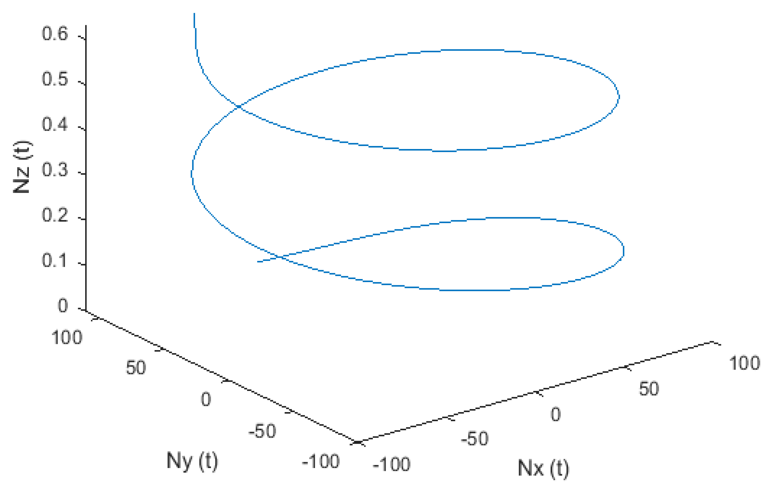
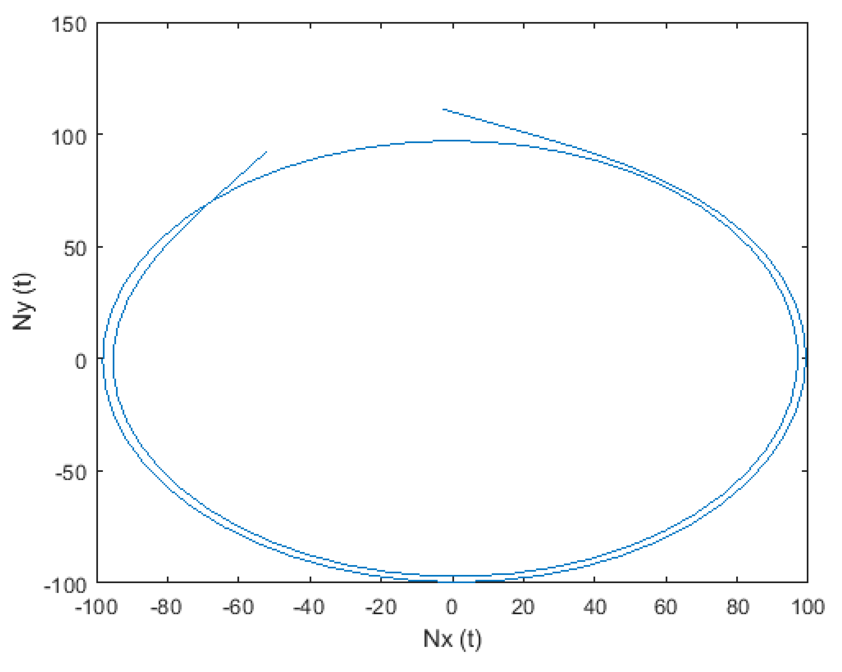
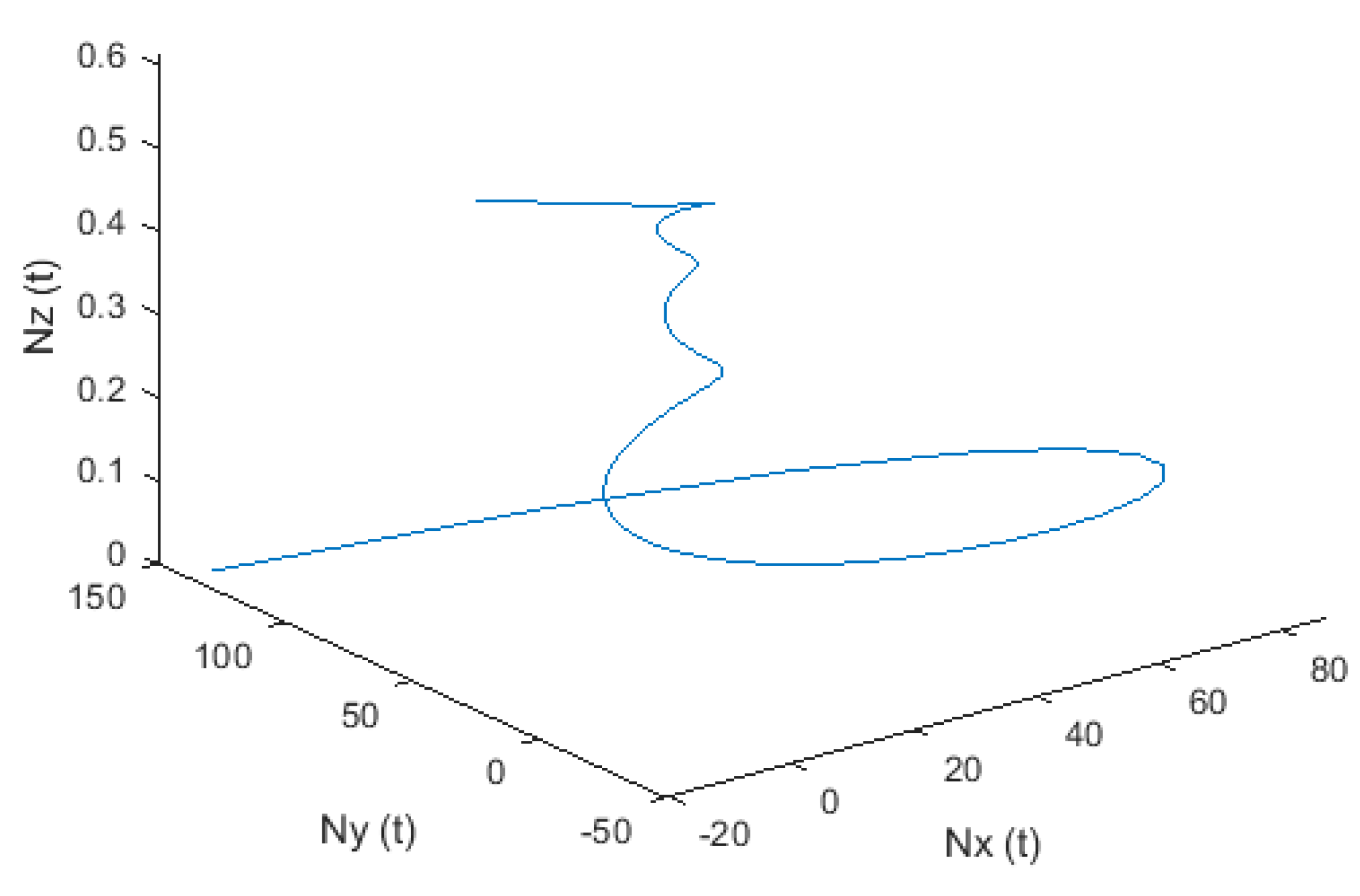
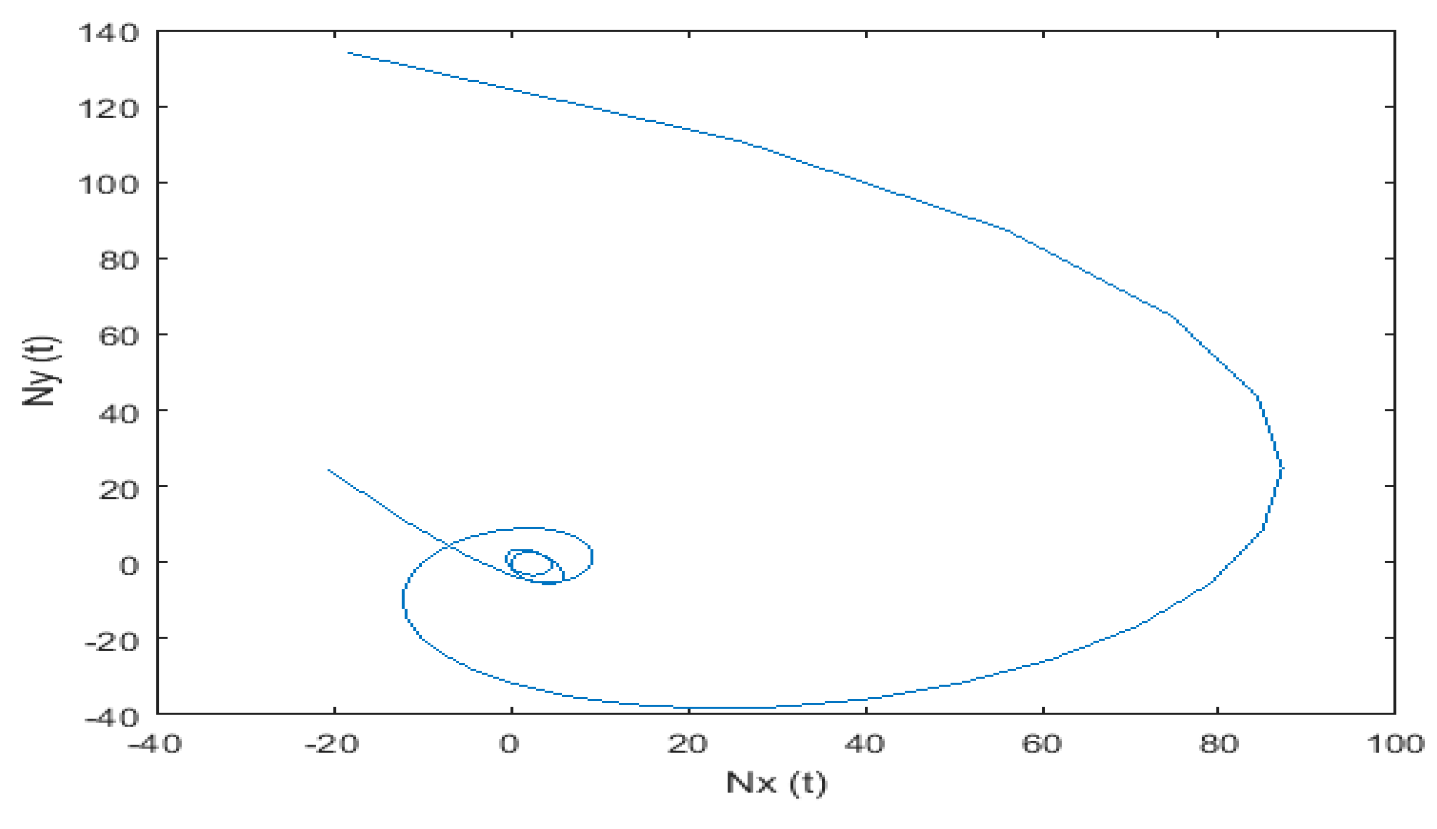
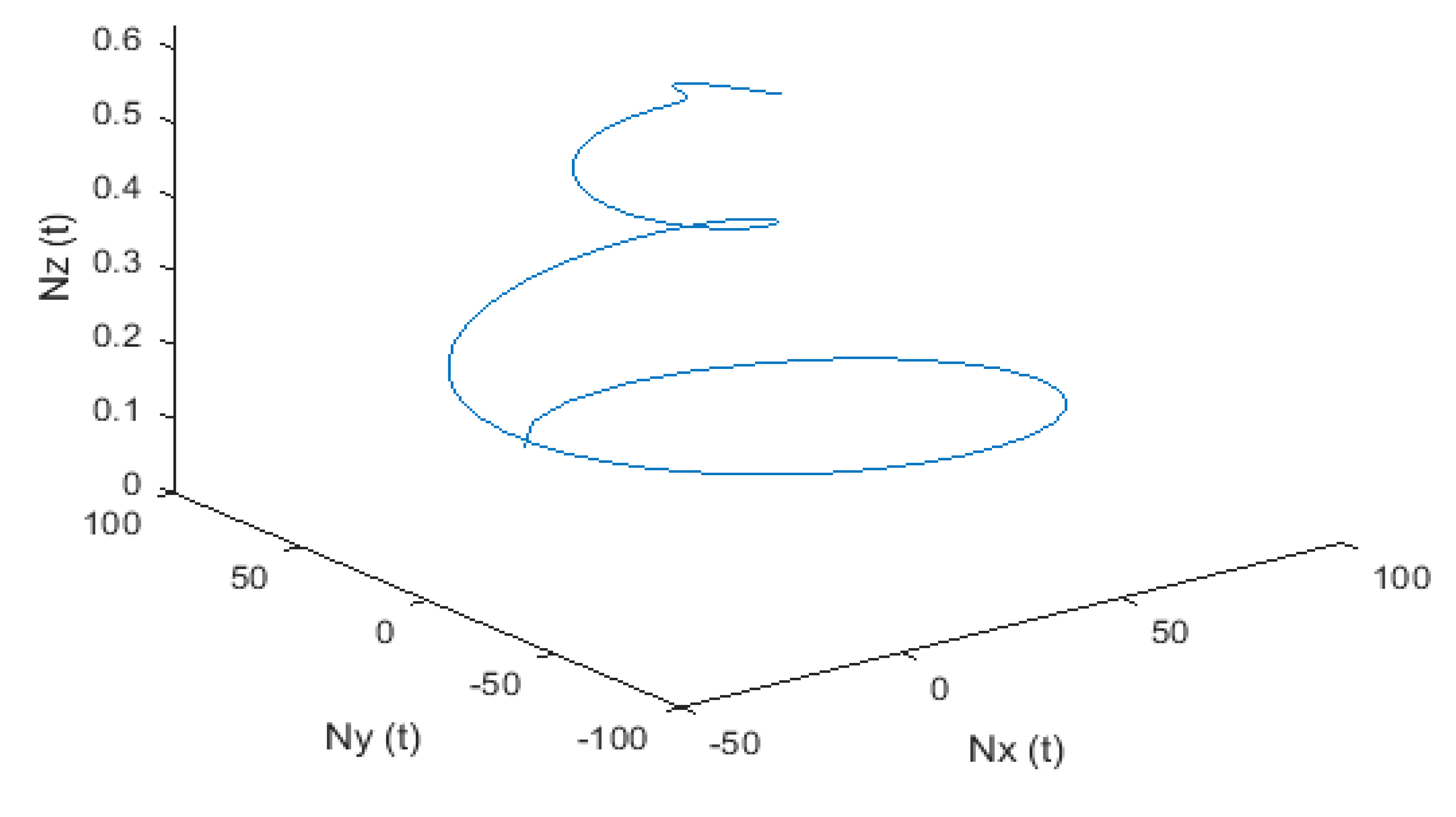
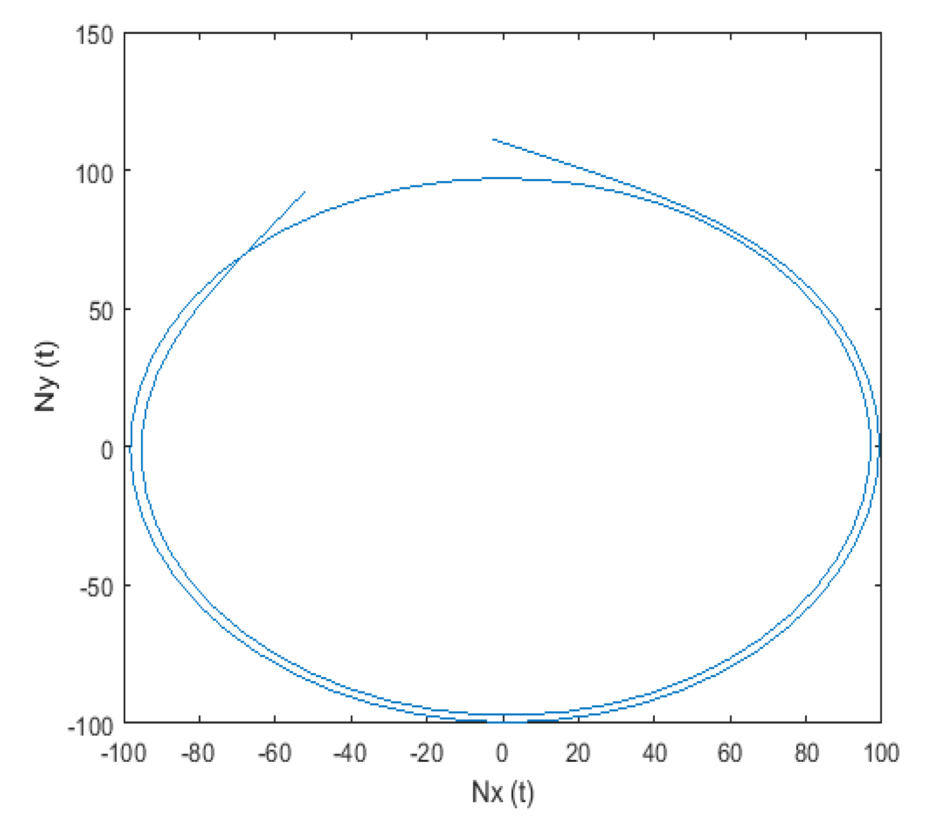
In this section, we will numerically simulate our results with known results. For each numerical simulation, we will consider i. c. and . In Figure 1 and Figure 2, we have presented 3D and 2D plots of the numerical solutions of the Bloch equation for integer order, respectively. These figures show the dynamics of for integer-order relaxation. In Figure 1, the entire trajectory of magnetisation is shown in 3D for integer order starting at i. c. and returning to . From Figure 2, it is clear that the magnetisation in direction increases with time, and the magnetisation in direction decreases with time.
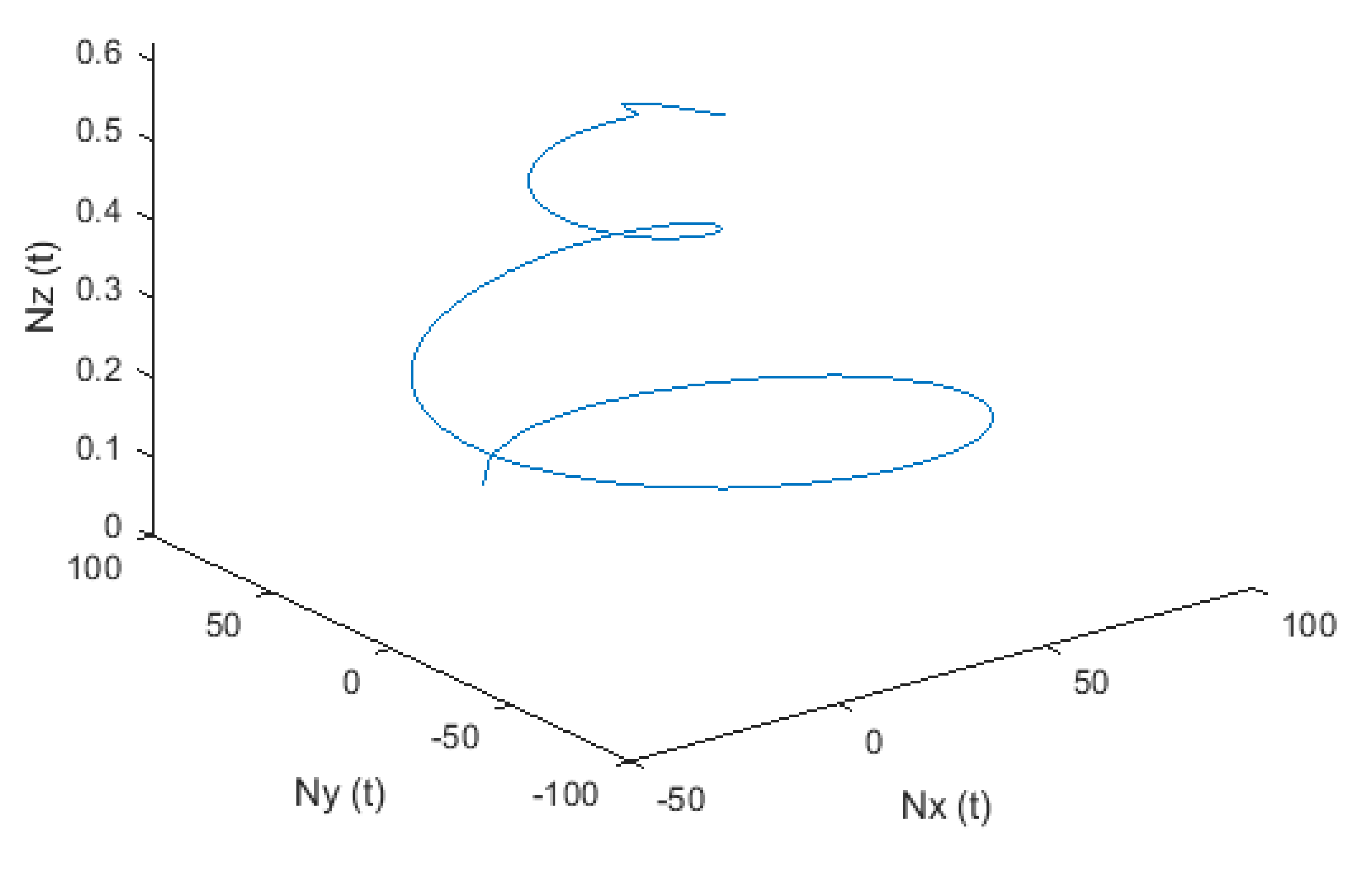
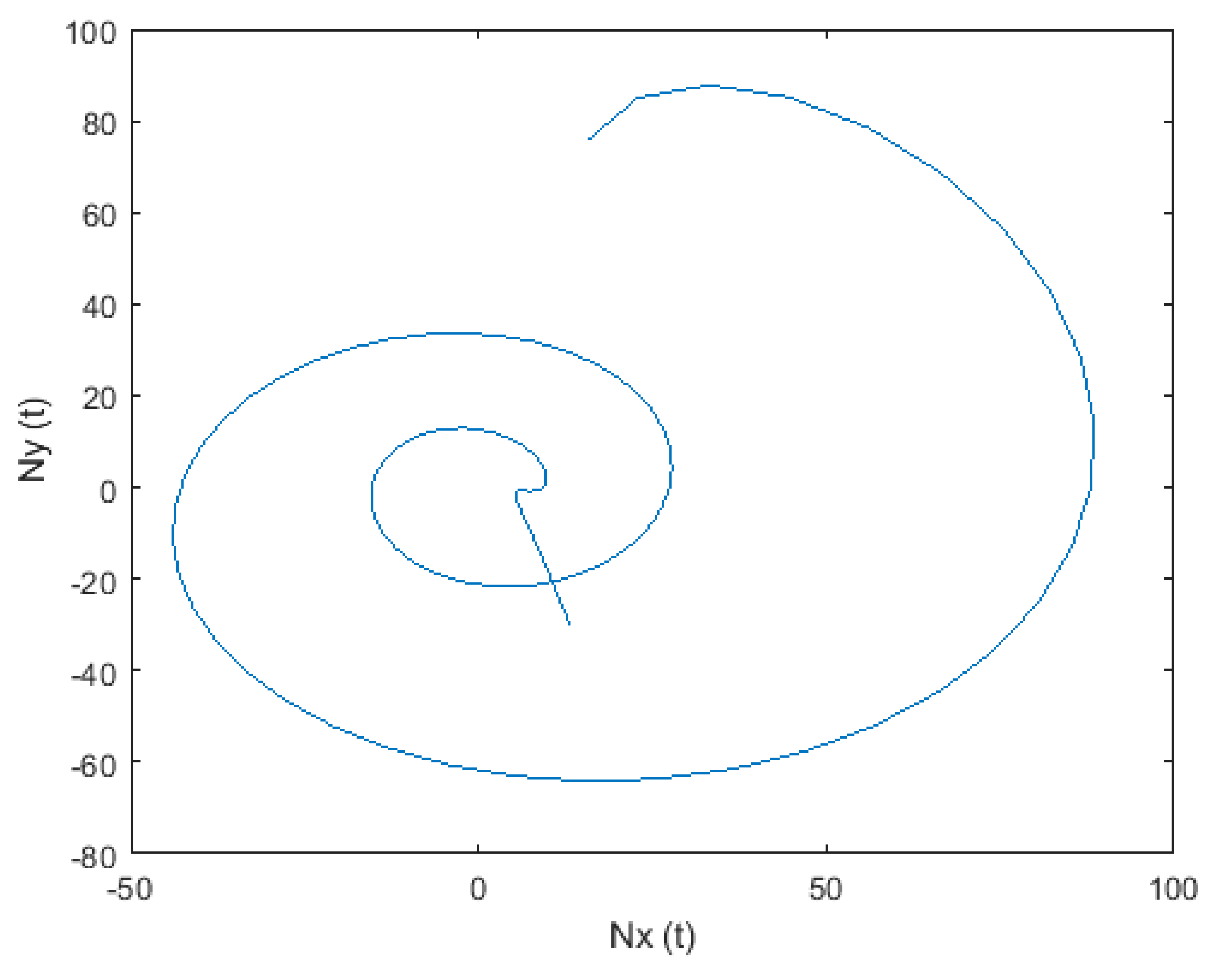
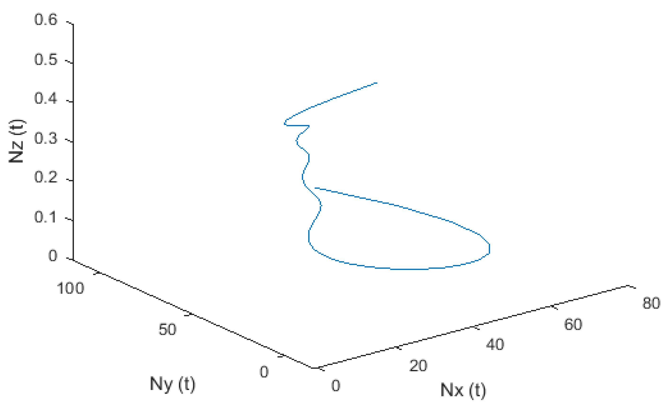
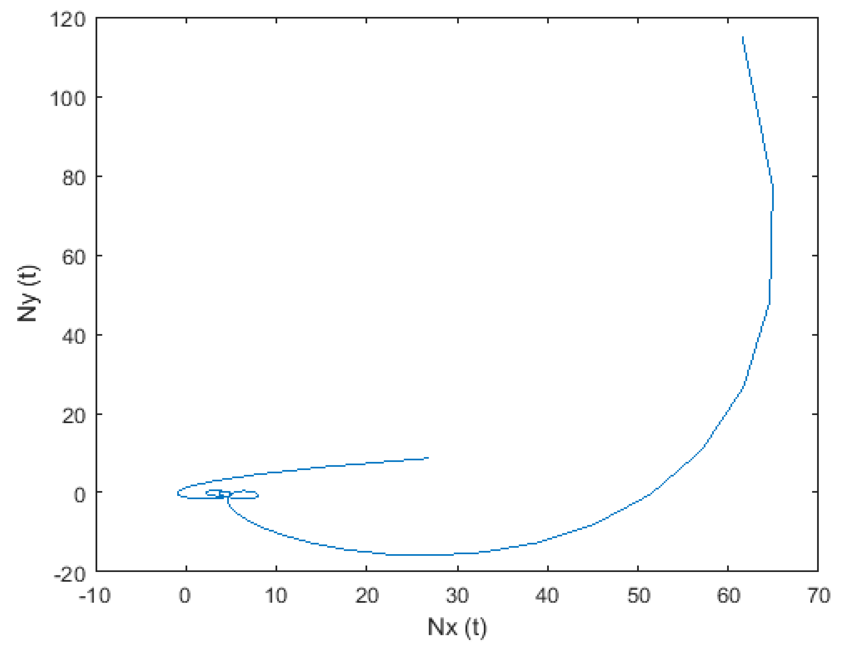
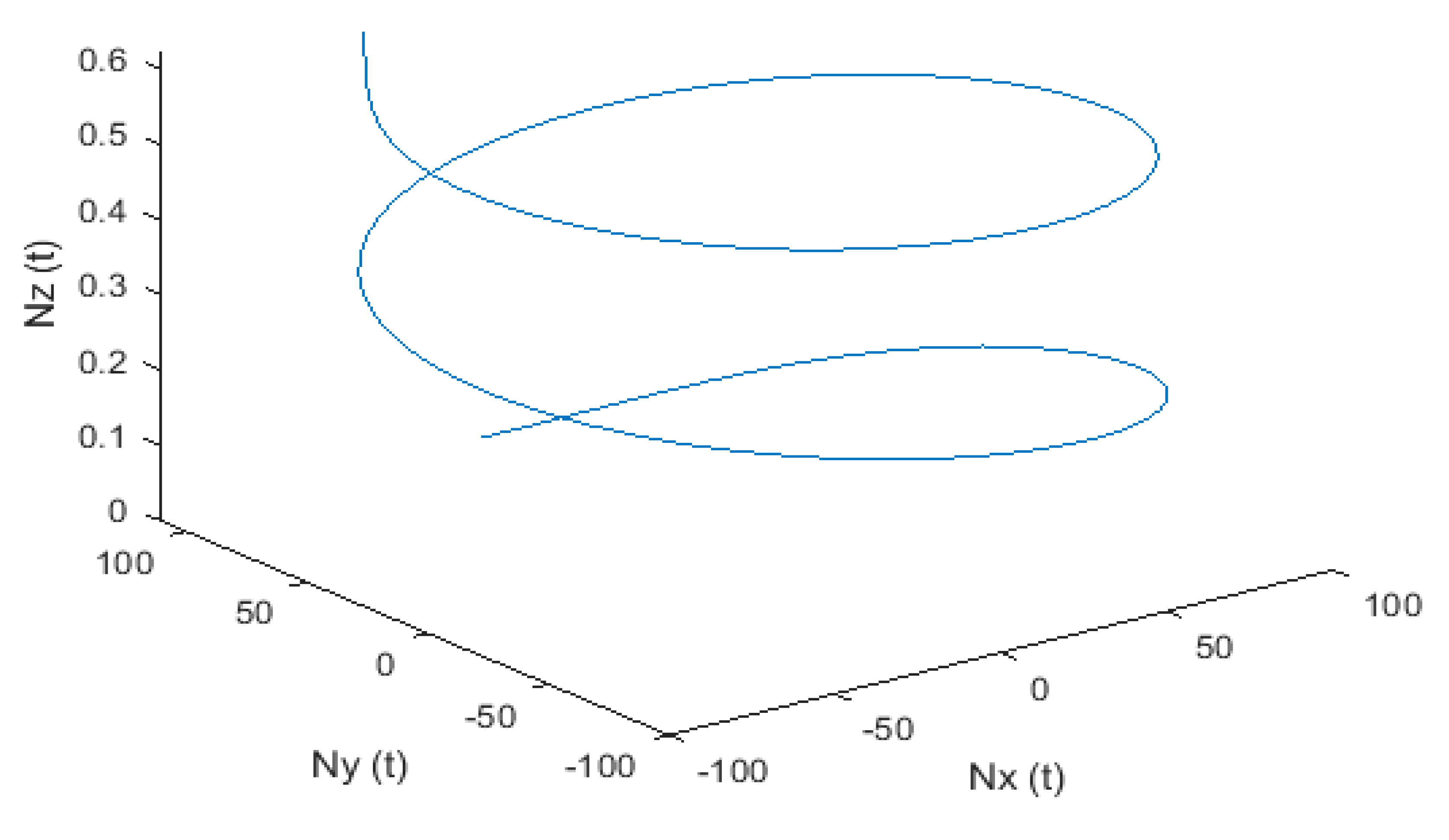
In Figure 3 and Figure 4, we have presented 3D and 2D plots of the numerical solutions of the Bloch equation for fractional order , respectively. These figures show the dynamics of for fractional-order relaxation. In Figure 3, the entire trajectory of magnetisation is shown in 3D for fractional order starting at i. c. and returning to . From Figure 4, it is clear that the magnetisation in direction increases with time, and the magnetisation in direction decreases with time.
In Figure 5 and Figure 6, we have presented the 3D and 2D plots of the numerical solutions of the Bloch equation for fractional order respectively. These figures show the dynamics of for the fractional-order relaxation. In Figure 5, the entire trajectory of magnetisation is shown in 3D for fractional order starting at i. c. and returning to . From Figure 6, it is clear that the magnetisation in direction increases with time, and the magnetisation in direction decreases with time.
In Figure 7 and Figure 8, we have presented the 3D and 2D plots of the numerical solutions of the Bloch equation for fractional order respectively. These figures show the dynamics of for the fractional-order relaxation. In Figure 7, the entire trajectory of magnetisation is shown in 3D for fractional order with the starting initially and returning to . From Figure 8, it is clear that the magnetisation in direction increases with time, and the magnetisation in direction decreases with time.
In Figure 9 and Figure 10, we have presented the 3D and 2D plots of the numerical solutions of the Bloch equation for fractional order respectively. These figures show the dynamics of for the fractional-order relaxation. In Figure 9, the entire trajectory of magnetisation is shown in 3D for fractional order starting at i. c. and returning to . From Figure 10, it is clear that the magnetisation in direction increases with time, and the magnetisation in direction decreases with time.
In Figure 11 and Figure 12 we have presented 3D and 2D plots of numerical solutions of Bloch equation for fractional order respectively. These figures show the dynamic of for fractional order relaxation. In Figure 11, the entire trajectory of magnetisation is shown in 3D for fractional order starting at i.c. and returning to . From Figure 12, it is clear that the magnetisation in direction increases with time, and the magnetisation in direction decreases with time.
In Figure 13 and Figure 14, we have presented the 3D and 2D plots of the numerical solutions of the Bloch equation for fractional order , respectively. These figures show the dynamics of for the fractional-order relaxation. In Figure 13, the entire trajectory of magnetisation is shown in 3D for fractional order starting at the initial level and returning to . From Figure 14, it is clear that the magnetisation in direction increases with time, and the magnetisation in direction decreases with time.
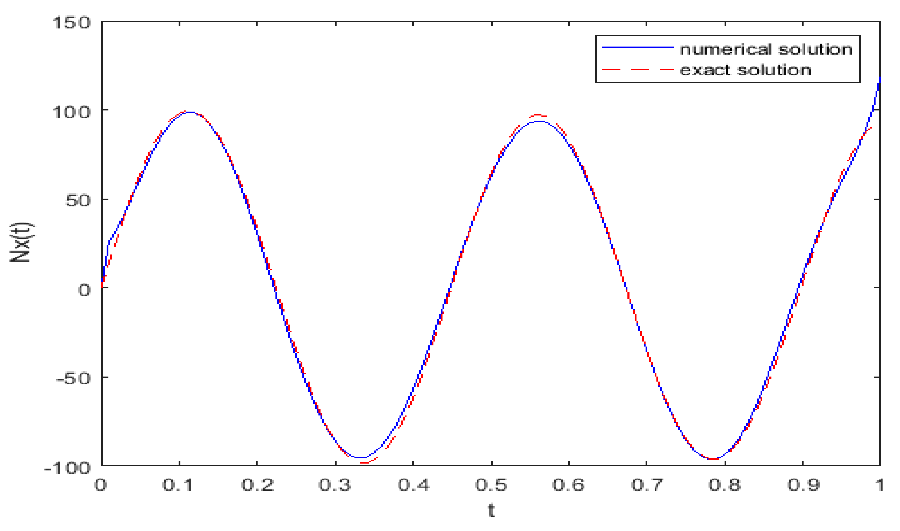
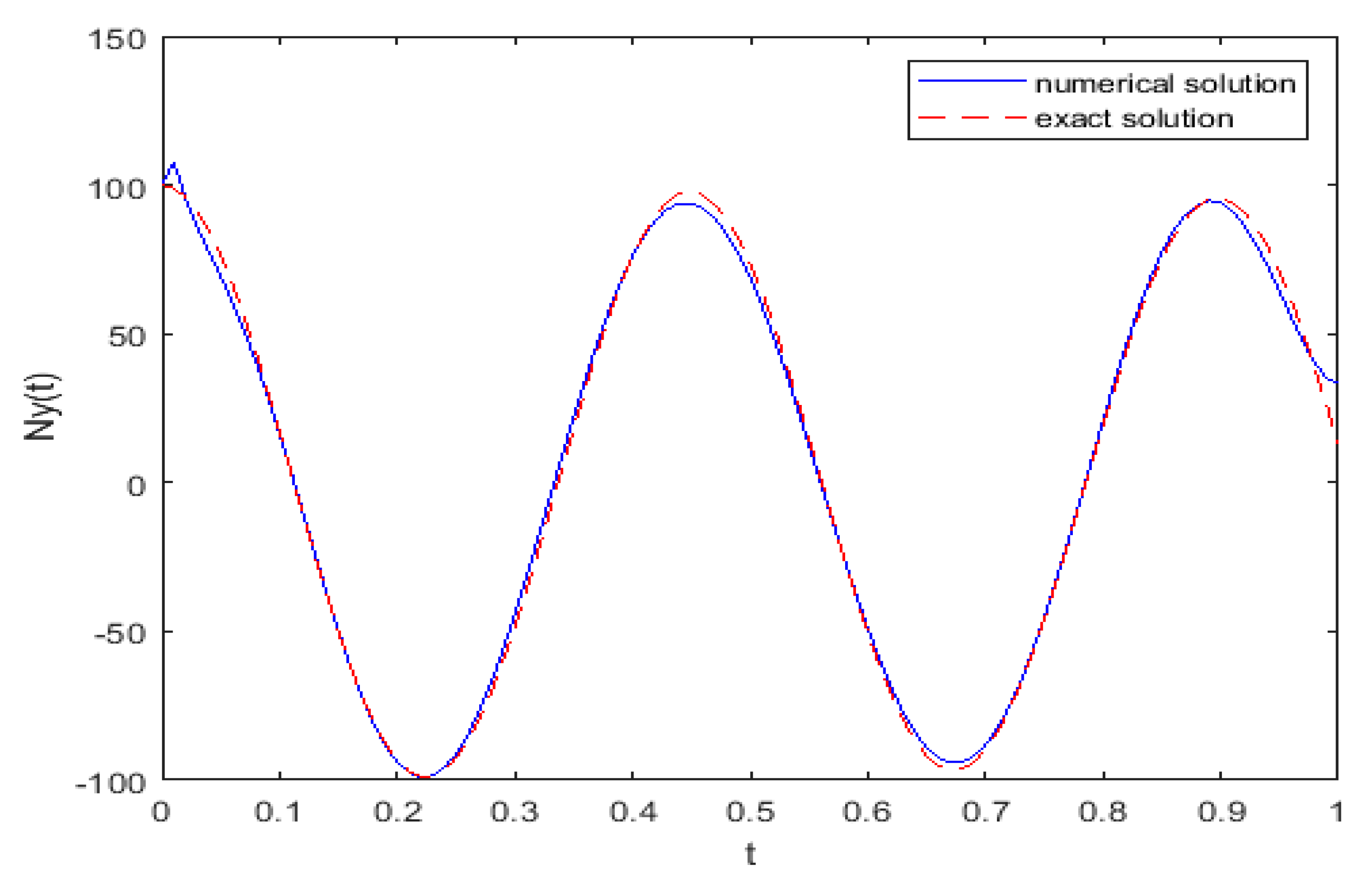
In Figure 15 and Figure 16, we have shown the numerical simulation of analytical and numerical solutions of the Bloch equation for and for integer order, respectively. From Figure 16, it is clear that the solution has periodic behaviour at low frequency. This solution varies periodically for and at low frequency.
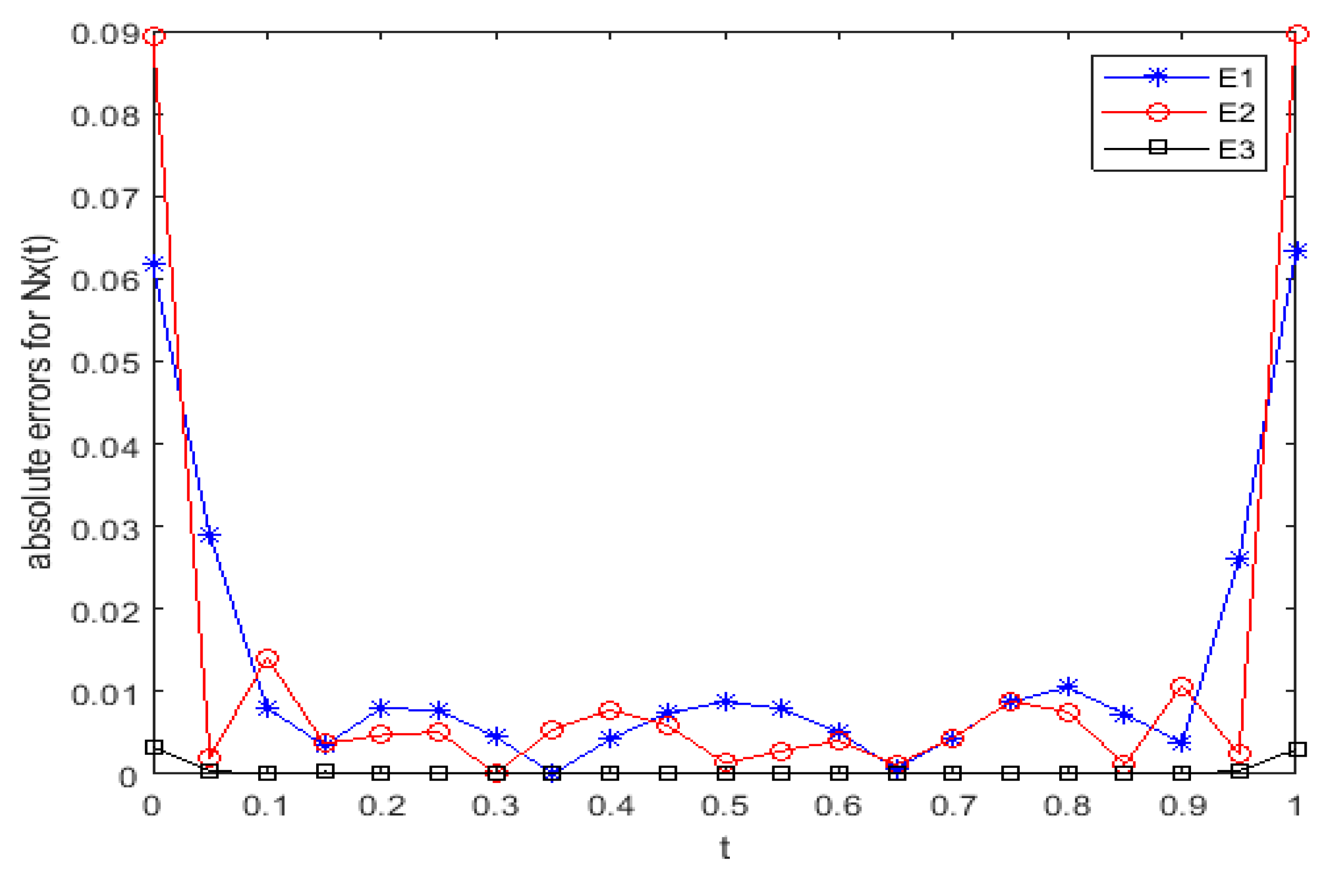
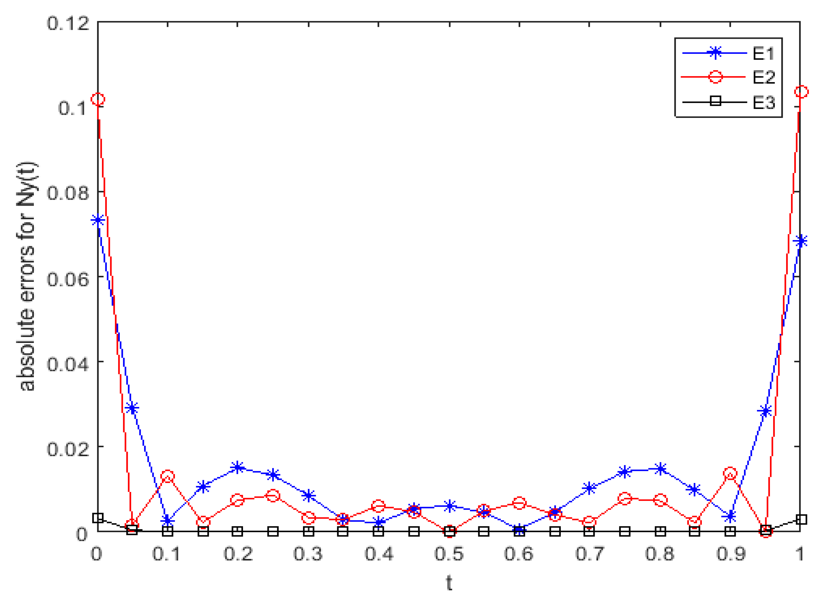
In Figure 17, Figure 18 and Figure 19, we have shown the absolute errors for , respectively, at different values of . In Figure 17, Figure 18 and Figure 19, the absolute errors are denoted by and for and 9, respectively. In all these figures, and are multiplied by and , respectively.
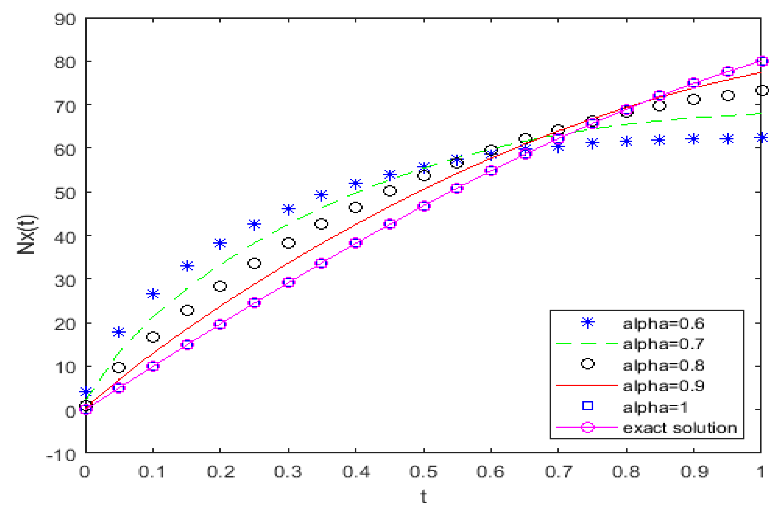
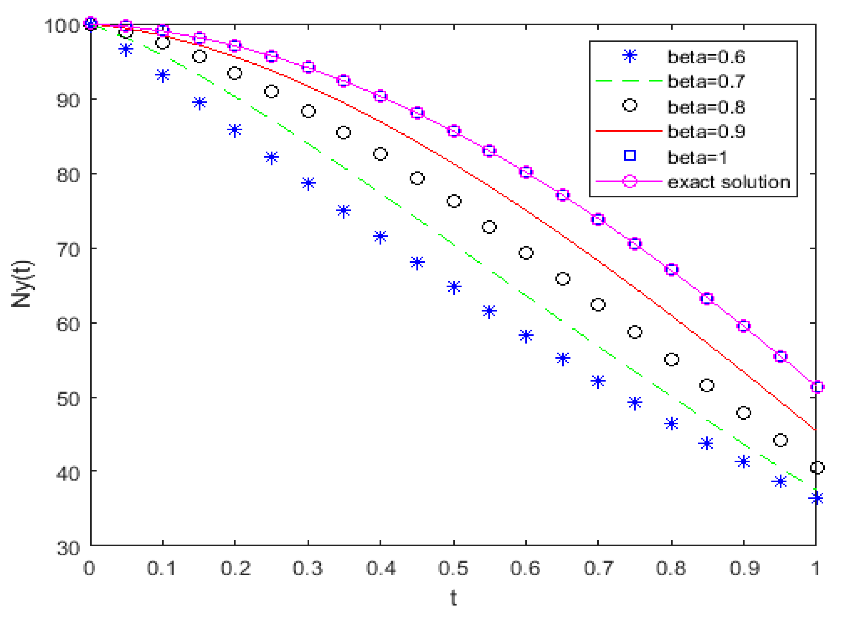
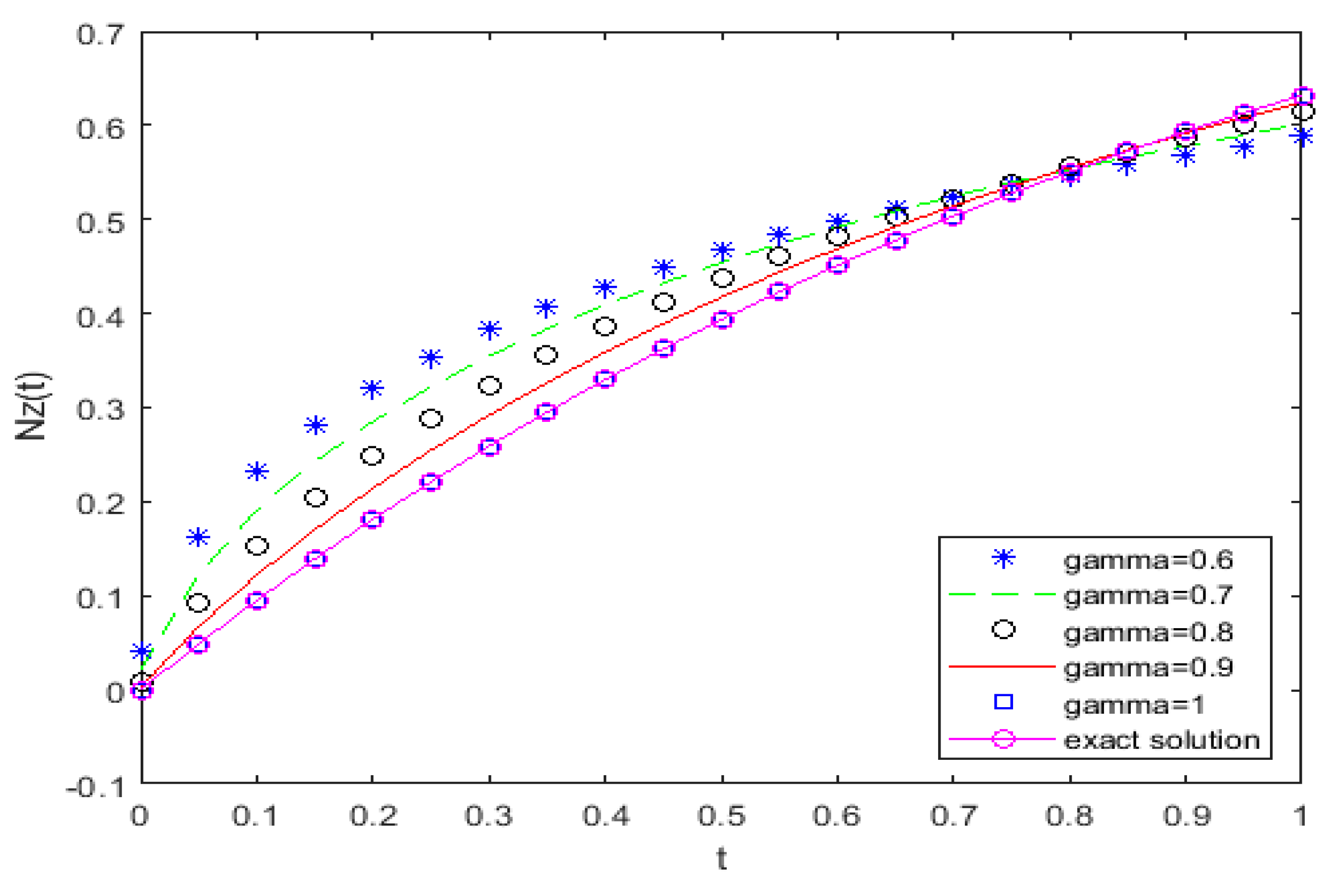
From these figures, we can see that the errors decrease with the increase of . In Figure 20, Figure 21 and Figure 22, we have shown the behaviour of the solutions of at different values of respectively. In Figure 20, Figure 21 and Figure 22, exact solution means the analytical solution for integer order Bloch equation as given by Equation (2).
From these figures it is clear that the solution varies consistently from non-integer order to integer order.
In Table 1, we have listed the maximum absolute errors () and the root-mean-square errors () for two different values of and at . We have calculated these errors for integer order by taking the exact solution as given by Equation (2).
From Table 1, it is detected that the errors decrease with the increase of .
6. Conclusions and Future Scope
In this paper, we have presented the numerical solution and the simulation for fractional-order and integer-order Bloch equations. Mathematical model for NMR allows us to explore and define magnetisation for spin dynamics at resonance frequency in a static magnetic field. Implementation of our proposed technique is easy in comparison to the existing methods because the operational matrices are easy to construct. The numerical section shows how the solution given by the used technique varies consistently at different values of non-integer-order time-derivatives. Moreover, for integer order, the solution by the used technique is identical to the exact solution for the Bloch equation. The error table shows the accuracy of the proposed method. For future work, we can construct operational matrices for different polynomials in order to attain better exactness.
Author Contributions
Both authors have equal contribution. All authors have read and agreed to the published version of the manuscript.
Funding
This research received no external funding.
Conflicts of Interest
The authors declare no conflict of interest.
References
- Bagley, R.L.; Torvik, P.J. A theoretical basis for the application of fractional calculus to viscoelasticity. J. Rheol. 1983, 27, 201–210. [Google Scholar] [CrossRef]
- Srivastava, H.M.; Shah, F.A.; Abass, R. An application of the Gegenbauer wavelet method for the numerical solution of the fractional Bagley-Torvik equation. Russ. J. Math. Phys. 2019, 26, 77–93. [Google Scholar] [CrossRef]
- Bagley, R.L.; Torvik, P.J. Fractional calculus in the transient analysis of viscoelasticity damped structures. AIAA J. 1985, 23, 918–925. [Google Scholar] [CrossRef]
- Robinson, A.D. The use of control systems analysis in neurophysiology of eye movements. Annu. Rev. Neurosci. 1981, 4, 462–503. [Google Scholar] [CrossRef] [PubMed]
- Singh, H. A new stable algorithm for fractional Navier-Stokes equation in polar coordinate. Int. J. Appl. Comput. Math. 2017, 3, 3705–3722. [Google Scholar] [CrossRef]
- Bohannan, G.W. Analog fractional order controller in temperature and motor control applications. J. Vib. Control 2008, 14, 1487–1498. [Google Scholar] [CrossRef]
- Panda, R.; Dash, M. Fractional generalized splines and signal processing. Signal Process 2006, 86, 2340–2350. [Google Scholar] [CrossRef]
- Kilbas, A.A.; Srivastava, H.M.; Trujillo, J.J. Theory and Applications of Fractional Differential Equations, North-Holland Mathematical Studies; Elsevier (North-Holland) Science Publishers: Amsterdam, The Netherlands, 2006. [Google Scholar]
- Li, X. Numerical solution of fractional partial differential equations using cubic B-spline wavelet collocation method. Adv. Comput. Math. Appl. 2012, 1, 159–164. [Google Scholar]
- Daftardar-Gejji, V.; Bhalekar, S. Solving fractional diffusion-wave equations using a new iterative method. Fract. Calc. Appl. Anal. 2008, 11, 193–202. [Google Scholar]
- Awojoyogber, O.B. Analytical solution of the time dependent Bloch NMR, flow equations: A translational mechanical analysis. Phys. A Stat. Mech. Appl. 2004, 339, 437–460. [Google Scholar] [CrossRef]
- Murase, K.; Tanki, N. Numerial solution to the time dependent Bloch equations revisited. Magn. Reson. Imaging 2011, 29, 126–131. [Google Scholar] [CrossRef] [PubMed]
- Leyte, J.C. Some solutions of the Bloch equations. Chem. Phys. Lett. 1990, 165, 231–240. [Google Scholar] [CrossRef]
- Yan, H.; Chen, B.; Gore, J.C. Approximate solutions of the Bloch equations for selective excitation. J. Magn. Reson. 1987, 75, 83–95. [Google Scholar] [CrossRef]
- Hoult, D.I. The solution of the Bloch equation in presence of varying B 1 field—An approach to selective pulse analysis. J. Magn. Reson. 1979, 35, 69–86. [Google Scholar] [CrossRef]
- Xu, Z.; Chan, A.K. A Near-Resonance solution to the Bloch equations and its application to RF pulse design. J. Magn. Reson. 1999, 138, 225–231. [Google Scholar] [CrossRef]
- Magin, R.; Feng, X.; Baleanu, D. Solving the fractional order Bloch Equation. Concepts Magn. Reson. Part A 2009, 34, 16–23. [Google Scholar] [CrossRef]
- Kumar, S.; Faraz, N.; Sayevand, K. A fractional model of Bloch equation in NMR and its analytic approximate solution. Walailak J. Sci. Technol. 2014, 11, 273–285. [Google Scholar]
- Singh, H. A New Numerical Algorithm for Fractional Model of Bloch equation in nuclear magnetic resonance. Alex. Eng. J. 2016, 55, 2863–2869. [Google Scholar] [CrossRef] [Green Version]
- Singh, H. Operational matrix approach for approximate solution of fractional model of Bloch equation. J. King Saud Univ. Sci. 2017, 29, 235–240. [Google Scholar] [CrossRef]
- Petráš, L. Modeling and numerical analysis of fractional-order Bloch equations. Comput. Math. Appl. 2011, 61, 341–356. [Google Scholar] [CrossRef]
- Ahmadian, A.; Chan, C.S.; Salahshour, S.; Vaitheeswaran, V. FTFBE: A numerical approximation for fuzzy time-fractional Bloch equation. In Proceedings of the International conference on fuzzy systems (FUZZ-IEEE), World Congress on Computational Intelligence, Beijing, China, 6–11 July 2014; pp. 418–423. [Google Scholar]
- Wu, J.L. A wavelet operational method for solving fractional partial differential equations numerically. Appl. Math. Comput. 2009, 214, 31–40. [Google Scholar] [CrossRef]
- Singh, H.; Srivastava, H.M.; Kumar, D. A reliable numerical algorithm for the fractional vibration equation. Chaos Solitons Fractals 2017, 103, 131–138. [Google Scholar] [CrossRef]
- Tohidi, E.; Bhrawy, A.H.; Erfani, K. A collocation method based on Bernoulli operational matrix for numerical solution of generalized pantograph equation. Appl. Math. Model. 2013, 37, 4283–4294. [Google Scholar] [CrossRef]
- Kazem, S.; Abbasbandy, S.; Kumar, S. Fractional order Legendre functions for solving fractional-order differential equations. Appl. Math. Model. 2013, 37, 5498–5510. [Google Scholar] [CrossRef]
- Singh, C.S.; Singh, H.; Singh, V.K.; Singh, O.P. Fractional order operational matrix methods for fractional singular integro-differential equation. Appl. Math. Model. 2016, 40, 10705–10718. [Google Scholar] [CrossRef]
- Singh, H.; Srivastava, H.M. Jacobi collocation method for the approximate solution of some fractional-order Riccati differential equations with variable coefficients. Phys. A Stat. Mech. Appl. 2019, 523, 1130–1149. [Google Scholar] [CrossRef]
- Singh, C.S.; Singh, H.; Singh, S.; Kumar, D. An efficient computational method for solving system of nonlinear generalized Abel integral equations arising in astrophysics. Phys. A Stat. Mech. Appl. 2019, 525, 1440–1448. [Google Scholar] [CrossRef]
- Singh, H.; Pandey, R.K.; Baleanu, D. Stable numerical approach for fractional delay differential equations. Few-Body Syst. 2017, 58, 156. [Google Scholar] [CrossRef]
- Srivastava, H.M. Fractional-order derivatives and integrals: Introductory overview and recent developments. Kyungpook Math. J. 2020, 60, 73–116. [Google Scholar]
Figure 1.
Numerical solutions of the Bloch equation with parameters: , , , , .

Figure 2.
Numerical solutions of the Bloch equation in plane with parameters: , , , .

Figure 3.
Numerical solutions of the Bloch equation with parameters: , , , .

Figure 4.
Numerical solutions of the Bloch equation in the plane with parameters: , , , .

Figure 5.
Numerical solutions of the Bloch equation with parameters: , , , .

Figure 6.
Numerical solutions of the Bloch equation in the plane with parameters: , , , .

Figure 7.
Numerical solutions of the Bloch equation with parameters: , , , .

Figure 8.
Numerical solutions of the Bloch equation in the plane with parameters: , , , .

Figure 9.
Numerical solutions of the Bloch equation with parameters: , , , .

Figure 10.
Numerical solutions of the Bloch equation in the plane with parameters: , , , .

Figure 11.
Numerical solutions of the Bloch equation with parameters: , , , .

Figure 12.
Numerical solutions of the Bloch equation in the plane with parameters: , , , .

Figure 13.
Numerical solutions of the Bloch equation with parameters: , , , .

Figure 14.
Numerical solutions of the Bloch equation in the plane with parameters: , , , .

Figure 15.
Numerical simulation of solutions of the Bloch equation for with parameters: , , , .

Figure 16.
Numerical simulation of solutions of the Bloch equation for with parameters: , , , .

Figure 17.
Errors for at , with parameters: , , , .

Figure 18.
Errors for at , with parameters: , , , .

Figure 19.
Errors for at , with parameters: , , , .

Figure 20.
Behaviour of the approximate solution of at , with parameters: , , .

Figure 21.
Behaviour of the approximate solution of at , with parameters: , , .

Figure 22.
Behaviour of the approximate solution of at , with parameters: , , .


Table 1.
Comparison of () and () errors at , for integer order solution.
| 2.0349 × 10⁻⁴ | 4.2101 × 10⁻⁸ | |
| 5.7209 × 10⁻⁶ | 9.2050 × 10⁻¹⁰ | |
| 1.9648 × 10⁻⁴ | 6.2953 × 10⁻¹⁰ | |
| 5.5559 × 10⁻⁶ | 6.2953 × 10⁻¹⁰ | |
| 1.7733 × 10⁻⁶ | 5.7426 × 10⁻¹⁰ | |
| 5.0010 × 10⁻⁸ | 6.8075 × 10⁻¹² |
© 2020 by the authors. Licensee MDPI, Basel, Switzerland. This article is an open access article distributed under the terms and conditions of the Creative Commons Attribution (CC BY) license (http://creativecommons.org/licenses/by/4.0/).
Share and Cite
MDPI and ACS Style
Singh, H.; Srivastava, H.M. Numerical Simulation for Fractional-Order Bloch Equation Arising in Nuclear Magnetic Resonance by Using the Jacobi Polynomials. Appl. Sci. 2020, 10, 2850. https://0-doi-org.brum.beds.ac.uk/10.3390/app10082850
AMA Style
Singh H, Srivastava HM. Numerical Simulation for Fractional-Order Bloch Equation Arising in Nuclear Magnetic Resonance by Using the Jacobi Polynomials. Applied Sciences. 2020; 10(8):2850. https://0-doi-org.brum.beds.ac.uk/10.3390/app10082850
Chicago/Turabian StyleSingh, Harendra, and H. M. Srivastava. 2020. "Numerical Simulation for Fractional-Order Bloch Equation Arising in Nuclear Magnetic Resonance by Using the Jacobi Polynomials" Applied Sciences 10, no. 8: 2850. https://0-doi-org.brum.beds.ac.uk/10.3390/app10082850
Note that from the first issue of 2016, this journal uses article numbers instead of page numbers. See further details here.