Article

Linear Parameter-Varying Model Predictive Control of AUV for Docking Scenarios

1
Naval Ship & Maritime Systems Engineering Department, Naval Ship & Maritime Systems Division, Mitsubishi Heavy Industries, Ltd., 6-53 Tsukuba-machi, Isahaya City 854-0065, Japan
2
Industrial Systems and Control, Ltd., Culzean House, 36 Renfield Street, Glasgow G2 1LU, UK
3
CIS Department, ICT Solution Headquarters, Mitsubishi Heavy Industries, Ltd., 5-717-1 Fukahori-machi, Nagasaki City 851-0392, Japan
4
Organization for Marine Science and Technology, Nagasaki University, 1-14 Bunkyo-machi, Nagasaki City 852-8521, Japan
5
Division of Mechanical Science, Nagasaki University Graduate School, 1-14 Bunkyo-machi, Nagasaki City 852-8521, Japan
*
Authors to whom correspondence should be addressed.
Submission received: 15 March 2021 / Revised: 6 May 2021 / Accepted: 7 May 2021 / Published: 11 May 2021
(This article belongs to the Special Issue New Trends in the Control of Robots and Mechatronic Systems)

Abstract

:
A control system for driving an Autonomous Underwater Vehicle (AUV) performing docking operations in presence of tidal current disturbances is proposed. The nonlinear model of the vehicle has been modelled in a Linear Parameter-Varying (LPV) form. This is suitable for the design of the control system using a model-based approach. The LPV model was used for a Model Predictive Control (MPC) design for computing the set of forces and moments driving the nonlinear vehicle model. The LPV-MPC control action is mapped into the reference signals for the actuators by using a Thrust Allocation (TA) algorithm. This was based on the nonlinear models for the actuators and their position and orientation on the vehicle’s hull. The structural decomposition of MPC and TA reduces the computational burden involved in computing the control law on-line on an embedded control board. Both MPC and TA algorithms use the vehicle’s linear and angular positions, and velocities that are estimated by an LPV based Kalman Filter (KF). The proposed control system has been tested in different docking scenarios using various tidal current disturbances acting on the vehicle as an unmeasured disturbance. The simulation results show the controller is effective in controlling the AUV over the range of control scenarios meeting the constraints and specifications.

1. Introduction

The control of an Autonomous Underwater Vehicle (AUV) is considered. This has no tether and is used for large-area subsea survey or seabed mapping. The AUV operating time is limited because the power source is an internal battery, typically a lithium ion secondary battery, and its energy is limited, even though battery technology has been improved recently. Launch and recovery from a surface ship may be needed for the continuous operation of the AUV for power supply and data uploading. This is an inefficient operation for the total mission and will be reflected in the operational cost. Moreover, the recovery of the AUV, which has no tether cable, is a troublesome and dangerous offshore operation.
For the improvement of the efficiency of AUV operations, there have been many research studies on the use of subsea docking stations [1,2,3]. In this case the AUV docks to the subsea docking station and power is supplied and data are transferred through subsea cables between the docking station and the surface ship.
In Reference [4], the concept of underwater docking using AUV and ROV (Remotely Operated Vehicle) docking stations was proposed. The operation involves the AUV moving close to the standby ROV docking station, stopping and hovering in the vicinity of the ROV, and then the docking station on the ROV capturing the AUV with the docking device. When the AUV and the ROV docking station are in a separate positional relationship, the respective positions can be obtained from the surface ship, controlling the ROV docking station using an ultra-short baseline (USBL) acoustic positioning system. This transmits information to the AUV using underwater acoustic communications. However, when the AUV is close to the ROV docking station, it is important for the AUV to transition to the optimum position and orientation. The ROV docking station can then easily capture the AUV in the limited view of the underwater camera. The concept here is to install a 3D imaging sonar on the AUV to estimate the position and the attitude of the ROV docking station. The transfer can then be achieved to the optimum position and attitude using an advanced hovering control [5,6]. In the following, we introduce new trajectory and attitude control for the AUV.
After estimating the orientation of the ROV docking station with a 3D imaging sonar, the AUV transitions to a final hovering position where the ROV docking station can easily capture it. It then holds a fixed point in a predetermined orientation, and awaits capture by the ROV docking station. During cruising at a certain speed or higher, the AUV position and attitude are controlled by the main thruster and the rudder. However, during low speeds, or holding at a fixed point, the hydrodynamic action from the rudder is insufficient, so the AUV is controlled by a plurality of side thrusters that generate thrust in the vertical and horizontal directions.
In this way, it is necessary to perform control by a number of actuators including a side thruster in order to shift the position and the attitude while decelerating the speed in a relatively short distance and finally holding a fixed target position. It is necessary to consider constraints for an actuator, such as a rudder, or side thruster, including limits on rudder angle and upper limits on thrust. Model Predictive Control (MPC) is often used for the optimal control of industrial systems with hard constraints but this is a relatively nonlinear process that is faster than many applications. The solution proposed is, therefore, tailored to the application.
The equations of motion are six degrees of freedom for the AUV. These are required for model predictive control. They have nonlinear characteristics for velocity and angular velocity given fluid dynamic and Coriolis forces. The actuator characteristics such as the fins and thrusters also have non-linear characteristics. If such a nonlinear and complex motion model is used directly for model predictive control the prediction stage results in an excessive computational load. It is not in general therefore suitable for real time control for a system such as an AUV.
Different solutions have been proposed for facing the AUV control by MPC. For example, in Reference [7], the MPC is applied to the trajectory tracking of an AUV and the equation of motion is limited to the motion in the horizontal plane. It is also linearized around a constant forward speed to reduce the computational load. In [8], the MPC is applied to the trajectory tracking of an AUV, where motion is limited to the nonlinear motion in the horizontal plane. The three forces (moments) are used to control the three degrees of freedom (u, v, r) distributed models, and ways to reduce computational load are considered for nonlinear MPC problems. In both these cases, the control problem is limited to the horizontal plane.
For the docking control problem there is a combination of a tracking/path following mode and finally a dynamic positioning control mode. In this latter case at the docking position the attitude in the vertical plane, pitch and the roll must be controlled. We therefore examined the transfer of position and attitude control, and then the dynamic positioning control for the six degrees of freedom model.
To reduce the computational load, the basic configuration of the control system is divided into two modules: an MPC control module for outputting the virtual force required to follow a predetermined position, speed, and attitude, and a Thruster Allocation (TA) module for determining the command value to each actuator required to generate the virtual force [9]. The TA problem is also involved in the dynamic positioning control of a ship. The calculation load is reduced by dividing a complicated optimization problem into the two more manageable optimization problems. In addition, a Kalman filter is implemented to estimate states and disturbances, such as tidal currents.
To reduce the computational load of the MPC control module, a Linear Parameter Varying (LPV) modelling approach was adopted [10,11]. The LPV-MPC can be treated as a linear problem, although it can represent a good approximation of a nonlinear model and the system matrices are parameter dependent and change with time. As a result, a linear quadratic programming problem can be generated, so that predictive control can be performed in real-time with reasonable economy. A method to compensate for the prediction error caused by using locally linear models, representing the inherently nonlinear model, was introduced. The proposed control system has been tested in simulation considering different docking scenarios featured by several tidal current acting on the vehicle as an external unmeasured disturbance.
The optimum control of the AUV for docking under the constraint conditions is a challenging problem. Furthermore, the critical hardware development items, such as the docking devices, were developed in parallel. Therefore, for the control system design, the control algorithm was developed for the concept model AUV, and was verified based on simulation. This paper reports the development and simulation verification of this control algorithm. The paper covers the modeling in Section 2, the control system in Section 3, the simulation results in Section 4, and the finally the conclusions in Section 5.

2. AUV Model

In this section, the nonlinear model of the AUV is described. The nonlinear equations describing vehicle and actuators are discussed in Appendix A. The rigid-body dynamics, actuators, sensors, and tidal current dynamics are described below.

2.1. AUV Rigid-Body Model

The equations of motion of the vehicle involve the rigid–body dynamic terms and components related to hydrodynamic forces and moments. The model includes the three main effects including restoring forces (depending on vehicle geometry and mass), the added mass (due to forced harmonic vehicle motion induced by force/moment pressure) and the damping terms (caused by skin friction and vortex shedding). The nonlinear dynamics model of the AUV may be represented in a compact matrix form introduced in Appendix A and expressed as follows:
M v ˙ + C v v + D v v + g η = τ A
where M is the mass matrix component, C represents the Coriolis effects, D represents the dumping effects, g corresponds to restoring forces and moments, τ A represents actuators thrust, v is the vector of linear and angular velocities and η is the array of linear and angular positions of the AUV. A detailed description of the elements of Equation (1) is given in Appendix A. The numerical values of the parameters are collected in Appendix B.

2.2. Actuators

The AUV is equipped with a set of actuators including fins and thrusters mounted in different positions over the vehicle hull, as shown in Figure 1.
The actuators include the main thruster, side thrusters (front and rear) and fins (stern planes and rudders). They are characterized in terms of the type, the position, and the orientation with respect to the vehicle-fixed reference frame and are described below. The combination of the forces and moments provided by the actuators determine the thrust to control the vehicle according to the controller command signals. A detailed description of the actuator dynamics for the AUV is presented in Appendix A and the parameter values are collected in Appendix B.

2.3. Sensors

The AUV is equipped with a set of INS sensors to measure the pose and velocities. The sensors measure position and orientation of the vehicle with respect to the inertial reference frame, and the instantaneous linear velocities with respect to the body-fixed reference frame. A delay of 20 ms affects the sensor measurements. The accuracy of the linear position sensors is 0.005 m and the linear velocities accuracy is 0.1 m/s. The angular position measurements have an accuracy of 5.42 × 10 5 rad., and the angular velocities accuracy is 5.42 × 10 3 rad/s.

2.4. Tidal Current Dynamics

In this work, the vehicle is subject to underwater currents that need countering. Considering the rigid-body AUV model of Equation (1), expressed in terms of the vehicle instantaneous velocities vector v, the tidal current is introduced in the model by considering the linear speed components of this disturbance with respect to the body-fixed reference frame ν T = u T , v T , w T , p T , q T , r T T . The relative velocity of the vehicle with respect to the tidal current can be computed as:
ν R = ν ν T
The effect of the tidal current can be introduced in the rigid body dynamics of Equation (1) by replacing ν with ν R so that:
M ν ˙ R + C ν R ν R + D ν R ν R + g η = τ A
Remark 1.
The tidal current ν T is constant in direction and velocity ( u ˙ T = v T ˙ = w T ˙ = 0   m / s 2 ), irrotational ( p T = q T = r T = 0   m / s ) and the vertical component of the current is neglectable ( w T = 0   m / s ).
Remark 2.
The tidal current speed V T = u T 2 + v T 2 is bounded such that V T 0 ,   0.514   m / s .
Remark 3.
The constant tidal current heading orientation is ψ T = ψ R O V + β where ψ R O V is the docking station heading and β 0.1745 , + 0.1745   r a d is constant.

3. AUV Control System

The proposed control system for driving the AUV is now presented. Initially, the architecture of the controller is described. The different aspects of the controller design are then introduced.

3.1. Control System Architecture

The proposed control system structure is shown in Figure 2. The nonlinear AUV system, including sensors and actuators (blue block) as described in the previous section, is affected by the tidal current (green block) speed ν T and the control system (grey block). The controller is composed of three main algorithms: a predictive control algorithm, an estimator and an allocation algorithm.
The Model Predictive Control (MPC, yellow block) computes the virtual control signals (forces and moments) τ V by solving an optimal control problem given the estimated state vector x ^ A U V and the control reference set-point signal vector r S P . A Kalman Filter (KF, orange block) is used to estimate the AUV system state x ^ A U V , by using the measured output signals y A U V and the virtual control signals τ V . The Thrust Allocation algorithm (TA, red block) converts the virtual control τ V , to a set of signals driving the actuators u A such that these provide a set of forces and moments minimizing the difference with τ V given the actuator limits and physical properties.
Predictive control methods normally involve a MPC algorithm to solve a single optimization problem, which computes the vector of future controls. This solution provides the sequence of control signals driving the actuators. It requires a single MPC design model involving the vehicle and actuator dynamics, and the actuator thruster allocation algorithm. This approach was investigated but an alternative route was taken to obtain a design that was more practical to implement.
In the following, a different control architecture was used to simplify the optimal problem by introducing two sub-problems, instead of one large optimization problem. This has the advantage that it provides a simpler (reduced number of optimization variables and control action constraints) optimization problem for the MPC. The TA policy also involves a simpler resources allocation problem that is to be solved only for the actual time instant. The controller structure avoids input and output constraints in the predictive controller, so that the MPC for this application is an unconstrained optimization problem that can be solved with a reduced computational effort with respect to other, constrained MPC problem solutions [12].

3.2. AUV Linear Parameter-Varying Model

To develop an MPC to control the AUV nonlinear dynamics, a design model permitting the prediction of the future AUV dynamics over a given future horizon is required. In this work, the design model is obtained in a Linear Parameter-Varying (LPV) form. The LPV modelling approach involves approximating a nonlinear dynamic model in a time-varying linear model form given the value of a set of measured/estimated variables. The LPV model of the AUV system involved represents the nonlinear dynamics model of Equation (6) in the following discrete time-varying state-space form:
x A U V k + 1 = A d k x A U V k + B d k τ V k + d d k
y A U V k = C d k x A U V k
where the state vector at the k -th time instance is:
x A U V k = x k , y k , z k , ϕ k ,   θ k ,   ψ k , u k , v k , w k , p k , q k , r k T
The measurement vector at the k-th time instant is:
y A U V k = x m k , y m k , z m k , ϕ m k ,   θ m k ,   ψ m k , u m k , v m k , w m k , p m k , q m k , r m k T
The virtual control signal vector provided by the MPC for driving the AUV rigid-body dynamics at the kth time instant is:
τ V k = X V k , Y V k , Z V k , K V k , M V k , N V k T
considering X V k , Y V k and Z V k virtual forces and K V k , M V k and N V k virtual moments generated over the x, y and z-axis of the body-fixed reference frame. The time-varying state-space variables of the LPV system are iteratively computed with respect to the nonlinear dynamics model of Equation (1), such that:
A t = 0 6 x 6 J η k M 1 ( C v t + D v t 0 6 x 6 M 1 ( C v t + D v t ;
B t = J η t M 1 M 1 ;
C t = I 12 x 12 , d t = J η t M 1 g η t M 1 g η t
are the LPV continuous-time state-space matrices discretized with respect to the controller sampling-time T s as A d k = A v t · T s + I , B d k = B η t · T s , C d k = C t and d d k = d η t · T s . Considering the LPV model of the vehicle, the vector of time-varying parameters is defined as ρ t = η t , v t T where A d k = A d ,   B d k = B d ρ k ,   C d k = C d ρ k and d d k = d d ρ k .

3.3. Linear Parameter-Varying Model Predictive Control

The MPC iteratively solves a finite-horizon, optimal control problem using a prediction model of the controlled system and an estimation of the current state. When the cost function is quadratic and constraints are affine, the LPV-MPC optimization problem to be solved at each time-step can be summarized as:
min u i = 1 N p 1 | | Q y A U V k + i | k r S P k | | 2 2 + j = 1 N u | | R Δ τ V k + j | k | | 2 2 + | | P ( y A U V k + N p | k r S P k | | 2 2
s . t .   x A U V ( k + i + 1 | k ) = A d k x k + i | k + B d k τ V k + i + d d k
y A U V k + i | k = C k x A U V ( k + i | k )
x A U V k | k = x ^ AUV k
τ V k + i + 1 = τ V k + i     f o r   i > N u
τ V k + i + 1 = τ V k + i + Δ τ V k + i + 1 f o r   i N u
Δ u V k + i D
τ V k + i U
y A U V k + i Y
N p N u
where P , Q and R the matrices for weighting the predicted output error, input rate and final output value (terminal weight), respectively, y A U V k + i | k is the output predicted at the i -th prediction step, r S P k is the reference output considered constant over the prediction/control horizon, Δ τ V k + j | k and τ V k + j | k are the predicted control input-rate and input-magnitude, respectively, N p is the prediction horizon and N u is the control horizon, D , U and Y are the convex sets on input rate, input and controlled output, respectively.
A standard LPV-MPC problem involves the assumption that the prediction model can be assumed constant over the prediction horizon, so that the model should match the real system for the first prediction step. Because the control action computed by MPC is mapped into the actuators control signals space by TA, there would be a mismatch between virtual forces and moments computed by MPC and real control forces and moments driving the AUV. This approximation introduces some sub-optimality in the solution, but enables the computational effort to be reduced, particularly with respect to more expensive nonlinear optimal control policies (e.g., nonlinear MPC). However, the controller performance can degrade because of the iterative introduction of an error in the prediction. To compensate for this problem, it is possible to iteratively evaluate the prediction of the plant model at least for the first prediction step.
The prediction error e p k can be iteratively computed by using the previous control effort so that,
e p k = x ^ k A d k 1 x ^ A U V k 1 + B d k 1 τ V k 1 + d d k 1
where x ^ A U V k is the state-estimate (provided by the Kalman filter), x ^ A U V k 1 is the state-estimate at the previous time step, τ V k 1 is the last computed control signal, d d k 1 is the last computed disturbance signal and A d k 1 ,   B d k 1 are the matrices describing the model at the previous time instant. The prediction error, computed as in Equation (22), can be introduced in the prediction model by updating the disturbance vector d d k iteratively, so that at each time instant it will be replaced by:
d ¯ k = d d k + e p k
with d d k the original disturbance vector. To reduce the computational complexity of the controller, the LPV-MPC problem can be represented as a condensed Quadratic Programming (QP) problem that can be implemented and solved on an embedded platform:
min z   1 2 z H k z + γ k F k z
s . t .   G k z h k γ k + w k
where z is the vector of optimization variables, γ k is the vector of MPC parameters belonging to a given set of interest, H k is a symmetric and positive definite matrix, F k is the linear cost–term matrix and G k , h k and w k are the terms defining constraints on input and output.

3.4. Thrust Allocation

The TA algorithm maps the set of virtual forces and moments τ V k into the space of actuator set-points u A k . The mapping is computed, at the controller sample times, given the instantaneous value of velocities (linear and angular) and orientation of the vehicle, also the orientation of the thrusters and the fins mounted on the vessel’s hull. The TA problem is formulated as a quadratic programming optimization problem with equality constraints:
min u   u c T W u A + u c T h
s . t . τ R t = G t u A
u A m < u A < u A M
where W is the weighting matrix on the quadratic term, h is the linear term, the vector of optimization variables grouping the actuator set-point values (main thruster, rudders and stern-planes, front and rear side-thrusters) is:
u A = u M , δ r 1 , δ r 2 , δ s 1 , δ s 2 ,   u R 1 , u R 2 , u R 3 , u R 4 , u F 1 , u F 2 , u F 3 , u F 4 T
and u A m and u A M are the vectors of minimum and maximum admissible values of the optimization variables (actuator saturations), respectively. The G t is the matrix representing a combination of optimization variables combining actuator forces and moments according their position on the vessel hull and vehicle’s pose:
τ V = X V X A , Y V Y A , Z V Z A , K V K A , M V M A , N V N A T
is the vector of reference moment and forces. It is computed considering the difference between virtual forces and moments ( X V , Y V , Z V , K V , M V , N V ) provided externally (from the MPC) and the effort provided by the interaction between actuators and the underwater environment, according to the vehicle’s layout and dynamics ( X A , Y A , Z A , K A , M A , N A ). These last terms are given by the resultant of the set of actuators, so that:
X A = 0
Y A = 1 2 Y u u δ r u v + 1 2 Y u r f u r
Z A = 1 2 Z u u δ s u w + 1 2 Y u r f u q
K A = 0
M A = 1 2 Y u r f u w + 1 2 M u q f u q
N A = 1 2 N u u δ r u v + 1 2 M u q f u r
The matrix G is a time-varying configuration matrix defined as:
G = G 11 0 0 0 0 G s 1 0 G Y G Y 0 0 G s 2 0 0 0 G z G z G s 3 0 G k G k G k G k G s 4 0 0 0 G m G m G s 5 0 G n G n 0 0 G s 6
with
G 11 = 0.46 u ρ D 0 3 / n k 1 + 0.66 ρ D 0 4   if   n k 1 u > = 0
G 11 = 0.46 ρ D 0 4   if   n k 1 u < 0
G Y = u 2 0.25 Y u u δ r
G z = u 2 0.25 Z u u δ s
G k = K u u δ r u 2 0.25
G m = u 2 0.25 Y u r f
G n = u 2 0.25 N u u δ r
G s = G s 1 , G s 2 , G s 3 , G s 4 , G s 5 , G s 6 T = 0 0 0 0 0 0 0 0 c α c α c α c α c α c α c α c α c α c α c α c α c α c α c α c α d d d d d d d d D F c α D F c α D F c α D F c α D R c α D R c α D R c α D R c α D F c α D F c α D F c α D F c α D R c α D R c α D R c α D R c α
where c α = cos α , and α = 45 degrees is the angular position of the thrusters with respect to the body-fixed reference frame.
Let u c k represent the actuator set-points computed at the actual iteration of the algorithm, u c k 1 the signals provided to the actuators at the previous time step and Δ u c m and Δ u c M the minimum and maximum values on the rate of change of the computed signals that define the constraints. These constraints were introduced in the TA problem above. Iteratively evaluating the value of the rate constraints, the magnitude constraints may be computed as:
u c i m k = max u c i m , u c i k 1 Δ u c i m
u c i M k = min u c i M , u c i k 1 + Δ u c i M
where the index i indicates the i-th actuator set-point signal and the related magnitude and rate constraint values.

3.5. Kalman Filter

A Kalman Filter (KF) has been considered to estimate the vehicle state vector. Because of the hard nonlinearities in the AUV dynamics, a Linear Parameter-Varying (LPV) version of the Kalman filter was developed to iteratively compute the angular velocities of the vehicle. The LPV-KF improves the standard linear KF by updating the state–space model of the system given the last measured value of the time-varying parameters (measured or estimated) that defines the system’s behavior [13,14,15]. The LPV-KF algorithm consists of the following steps:
S k = C d k P K F k | k 1 C d T k + R K F
L k = P K F k | k 1 C d T k S 1 k
y ˜ A U V k = y A U V k C d k x ^ A U V ( k | k 1 )
x ^ A U V k | k = x ^ A U V k | k 1 + L k y ˜ A U V k
P K F k | k = P K F k | k 1 L k S k L T k
x ^ A U V k + 1 | k = A d k x ^ A U V k | k + B d k τ V k + d d k
P K F k + 1 | k = A d k P K F k | k A d T k + Q K F
where matrices R K F and Q K F describe the variances of the measurement and the process noise terms. In the current problem they are assumed constant and defined during the algorithm set-up. The covariance matrix P K F and the system states are evaluated on-line iteratively.

4. Simulation Result

In this section, simulation results are presented. The AUV represented by the nonlinear dynamic model is driven to the docking position, where the docking station can catch it. The AUV model, the environment operating scenario and the control system was developed within the MATLAB/Simulink environment. The set of different simulation modules, functions and subsystems are described in Section 3 and Section 4 and in Appendix A, using the parameters collected in Appendix B.
The effect of environmental conditions can change when performing such a task, and in the following two sets of simulation results are given. The first test considers an environmental scenario with no tidal current, so that the vehicle is driven in ideal conditions. The second test considers the AUV performing the docking task in the presence of a tidal current with a speed V T = 0.514 m/s and oriented with an angle β = 0.1745 rad with respect to the final docking position heading angle. The control system used in the following has the tuning parameters defined as in Table 1.

4.1. No Current Test

The results of the first test, without any tidal current acting on the vehicle, are first presented. The objective of this test was to evaluate the performance of the AUV when moving to the docking position in zero current ideal conditions. The measured linear and angular positions of the controlled vehicle during the test are shown in Figure 3. This result shows the ability of the control system to drive the vehicle to the docking station meeting point in terms of linear and angular positions. The steady-state tracking errors in vertical position and in the pitch-angle are due to the mismatch between the actuators’ nonlinear model and the LPV design model. The mismatch causes an error in mapping the MPC control action into the actuator control signals space. Despite this mismatch, the performance of the controlled system satisfies the design specification.
The control actions driving the AUV actuators and computed by the TA policy are shown in Figure 4 that shows the main thruster control signal with respect to the saturation and backlash characteristics of the actuator. This reveals that the control signal managed by the TA satisfies the saturation (±2000 rpm) limit values and is adjusted to values (±400 rpm) due to the backlash. The main thruster control signal jumps between the limits of the backlash zone (±400 rpm), as defined in the control policy. When the MPC controller computes a large control effort to be provided by this thruster, the TA policy maps it into a control signal satisfying the saturation max/min constraints (e.g., at time t = 5 s).
Figure 5 shows the signals controlling the AUV fins, as they are driven almost symmetrically by the TA, such that for the rudders the control signal trajectory is different only for t = 8 s, whereas for the stern planes the control signals are coincident. Furthermore the fin controls satisfy the related constraints. Finally, in Figure 6 and Figure 7 the control signals are shown to drive the side thruster within the saturation limits. The control policy correctly drives the thrusters, despite the nonlinearities and constraints for the actuators. The fins and side thruster results show how the control system is able to generate the actuator control signals that satisfy the specified constraints.

4.2. Max Current Test

In the following the control system is tested by driving the AUV as before, but introducing the effect of the tidal current acting on the vehicle movement. The dynamics have been set to provide the worst case operating conditions (according to the specifications provided) by considering the maximum angular orientation ( β = 0.1745 rad) with respect to the final docking position and the maximum current speed ( V T = 0.514 m/s) acting on the opposite direction with respect to the vehicle’s orientation. The performance is shown in Figure 8, which reveals the variables controlled with respect to the set-point positions. Compared with the previous results, the performance indicates the effect of the current that increases oscillations. Despite this effect, the control system has the ability to control the system in this worst case scenario, maintaining the settling time and the steady-state performance. Figure 9 shows the main thruster control signal, where the current disturbance effect includes the additional oscillations.
Figure 10 shows the fin control signals. Compared to the previous fin controls, the stern plane signals are particularly affected by the tidal current, due to their effect on the AUV dynamics. Finally, in Figure 11 and Figure 12 the side thrusters’ performance is shown. In this control scenario, the constraints are satisfied, and the control signals accommodate the saturation and backlash. The stabilization of the vehicle in the docking position satisfies the design specifications, with limited oscillations within the accuracy range of the sensors.
Due to the presence of the current forces, these control signals are more aggressive. In fact, when the vehicle reaches zero forward speed, only the side thrusters and main thruster are used to maintain the required positions opposing the current forces.

5. Conclusions

The modelling and control of an Autonomous Underwater Vehicle (AUV) in a docking task was presented. The nonlinear dynamics model of the AUV was developed for the vehicle dynamics, actuators and sensor characteristics, and the effect of tidal currents acting on the vehicle was treated as an unmeasured disturbance. A control system based on an optimal predictive constrained control design approach was developed [16].
The control system is composed of three major subsystems. A Thrust Allocation (TA) algorithm subsystem was based on the models of the actuators. A Model Predictive Control (MPC) block was designed using a Linear Parameter-Varying (LPV) model of the AUV derived from the nonlinear model of the vehicle. A time varying Kalman Filter (KF) was used to estimate the state of the system. The control system performance was tested by driving the AUV over a set of control scenarios featuring different tidal current disturbance conditions. The results illustrated that the proposed controller could control the vehicle effectively in the docking task. Further developments involve the integration of the proposed control system within an advanced path planning policy that can minimize energy while approaching the docking station.
Mitsubishi Heavy Industries is also developing the AUV prototype for a docking technology demonstration based on the concept shown in Figure 1. This is in parallel with this study, which is called “Naminow-D”. The “Naminow-D” study has the addition of side thrusters and docking devices to the existing mono-axial propulsion AUV “Namiow”. The side thrusters and docking devices, including the underwater wireless power receiver, are installed externally to minimize the development cost. Figure 13 shows the “Naminow-D” under functional testing in the water tank.
Future studies will require physical parameter modifications, changes to the control software for implementation into embedded computer systems, and the sea trials, including comparison with simulation results.

Author Contributions

This study group consists of Japanese team and Scottish team. Japanese team mainly takes part of AUV and docking conceptualization and Scottish team takes part of development of control algorithm. And both team validated the results. In Japanese team, H.U. initiated and managed all of this study project, and contributed of AUV conceptualization and investigation of AUV and docking system. I.Y. supervised AUV and docking system. M.T. contributed conceptualization of AUV. K.E., Y.Y. and A.M. contributed the validation, and K.E. supervised in Japanese side. In Scottish side, G.M.v.d.M. managed the Scottish team, and M.J.G. supervised development of control algorithm. L.C. and P.M. contributed the development of control algorithm, such as conceptualization, formal analysis, Investigation, Methodology and Software. L.C. also contributed validation of the all of analysis result. The original manuscript was written by H.U., L.C. and P.M. And all of authors reviewed and edited the manuscript. All authors have read and agreed to the published version of the manuscript.

Funding

This research was funded by Nippon Foundation, Grant Number 2019524843.

Institutional Review Board Statement

Not Applicable.

Informed Consent Statement

Not Applicable.

Data Availability Statement

Data is contained within the article.

Conflicts of Interest

The authors declare no conflict of interest.

Appendix A

In this appendix, the AUV nonlinear dynamics model and related subsystems are presented. The model consists of reference frames definition, vehicle rigid-body dynamics and actuators’ models. The parameters for the AUV model that are not defined in this appendix are reported in Appendix B.
The AUV dynamics are defined by a set of nonlinear equations with respect to two coordinate reference frames termed the earth-fixed (inertial) and body-fixed frames. The inertial reference frame is used to represent vehicle pose (position and orientation). The body-fixed reference frame is used for velocities (linear and angular) and has its origin coincident with a center of buoyancy that moves/rotates together with the AUV. The velocities in the body-fixed frame are ν = u , v , w , p , q , r T with ν 1 = u , v , w T linear surge, sway and heave velocity and ν 2 = p ,   q , r T angular roll, pitch and yaw speed. The position of the AUV in the inertial reference frame is η = x ,   y ,   z ,   ϕ ,   θ ,   ψ T with η 1 = x ,   y ,   z T linear position and η 2 = ϕ ,   θ ,   ψ T angular orientation.
η 1 ˙ = J 1 η 2 ν 1
J 1 η 2 = c ψ c θ s ψ c Φ + c ψ s θ s Φ s ψ s Φ + c ψ c Φ s θ s ψ c θ c ψ c Φ + s Φ s ψ s θ c ψ s Φ + s θ s ψ c Φ s θ c θ s Φ c θ c Φ
η 2 ˙ = J 2 η 2 ν 2
J 2 η 2 = 1 t θ s Φ t θ c Φ 0 c Φ s Φ 0 s Φ / c θ c Φ / c θ
where s α = sin α ,   c α = cos α and t α = tan α . Equations (A1)–(A4) can be written in compact form such that η ˙ = J η 2 ν with J η = d i a g J 1 η 2 , J 2 η 2 .

Rigid-Body Dynamics Model

The nonlinear dynamics model of the AUV is formulated in a compact matrix form [14] as:
M v ˙ + C v v + D v v + g η = τ A
where M is the matrix of the rigid-body mass. In submerged vehicles it is defined as M = M R B + M A M with M R B the constant rigid-body inertia matrix and M A M is the added inertia matrix. The M R B is parametrized in the form:
M R B = m I m   s r G m   s r G I 0
Further, m is the mass of the vehicle, I is a 3 × 3 identity matrix, s · is the matrix cross product operator, r G is the vector of distances of the centre of gravity from the origin of the body-fixed reference frame (in the considered model the centre of buoyancy), and I 0 is the inertia tensor with respect to the body-fixed reference frame origin. The M A M is the added mass matrix (or added inertia matrix) used to model the effect of the water displaced by the vehicle during motion. It is composed of a set of constant coefficients, such that M ˙ A M = 0 and:
M A M = X u ˙ X v ˙ X w ˙ X p ˙ X q ˙ X r ˙ Y u ˙ Y v ˙ Y w ˙ Y p ˙ Y q ˙ Y r ˙ Z u ˙ Z v ˙ Z w ˙ Z p ˙ Z q ˙ Z r ˙ K u ˙ K v ˙ K w ˙ K p ˙ K q ˙ K r ˙ M u ˙ M v ˙ M w ˙ M p ˙ M q ˙ M r ˙ N u ˙ N v ˙ N w ˙ N p ˙ N q ˙ N r ˙
The coefficients for the previous added inertia matrix M A M , e.g., Y u ˙ Y / u ˙ = Y u d , are provided in the AUV specifications. Note that for an AUV this matrix is strictly positive. In Equation (A5) the term C v is the matrix of Coriolis and centripetal terms. Two terms are used to describe these effects, so that C v = C R B v + C A v with C R B v representing the skew-symmetrical parametrization of constant mass:
C R B v = 0 s M 11 v 1 + M 12 v 2 s M 11 v 1 + M 12 v 2 s M 21 v 1 + M 22 v 2
and C A M v represents the effect of the added mass due to the centripetal and Coriolis effects, also defined according to the skew-symmetrical parametrization:
C A M v = 0 s A 11 v 1 + A 12 v 2 s A 11 v 1 + A 12 v 2 s A 21 v 1 + A 22 v 2
with terms A i j ( i , j = 1 , 2 ) computed as for the added mass matrix. The extended form for of C A M v has the same structure as C R B v .
In addition, in Equation (A5) the term g η is the vector of restoring forces and moments. The gravitational force is defined as W = m g (that is the weight force acting on the vehicle due to the gravity g acting on the mass m ), the buoyancy is B = ρ 𝛻 g , where ρ is the fluid density and 𝛻 is the total volume of fluid displaced by the vehicle. Let r g = x g , y g , z g T denote the position of the centre of gravity and r B = x B , y B , z B T denote the centre of buoyancy with respect to the body-fixed reference frame. The restoring forces and moments g η = X R , Y R , Z R , K R , M R , N R T may then be computed as:
X R = W B sin θ
Y R = W B cos θ sin Φ
Z R = W B cos θ cos Φ
K R = y g W y B B cos θ cos Φ z g W z B B cos θ sin Φ
M R = z g W z B B sin θ + x g W x B B cos θ cos Φ
N R = x g W x B B cos θ sin Φ y g W y B B sin θ
The matrix of hydrodynamic damping terms is D v in Equation (A5). The hydrodynamic damping factors for marine vehicles may be classified as potential damping, viscous damping, wave drift damping, vortex shedding damping and lifting forces. The proposed model considers a nonlinear representation of damping effects with respect to instantaneous vehicle velocities, such that D v = X D , Y D , Z D , K D , M D , N D T with
X D = X u u u u
Y D = Y v v v v + Y r r r r + Y L
Z D = Z w w w w + Z q q q q + Z L
K D = K p p p p
M D = M q q q q + M w w w w + M L
N D = N r r r r + N v v v v + N L
The set of actuators include the main thruster, side thrusters (front and rear) and fins (stern planes and rudders). They are characterized in terms of the type, the position and the orientation with respect to the vehicle-fixed reference frame and described below.
The main thruster is positioned at the stern of the vehicle, aligned with the x-axis of the body-fixed reference frame, but it cannot provide forces, or moments, different from the force over this axis. The force generated by this thruster depends on the control action and its dynamics include different nonlinearities. The generated force X M is modelled by the following relationship:
X M = k t J ρ n 2 D 0 4 ω n 2 s 2 + 2 s ω n ζ + ω n 2
where ρ = 1024   k g m 3 is the water density, u M = n rpm is the control input (the required rotation speed), D 0 = 0.152   m is the nominal thruster diameter, k t J represents the nonlinear relationship between actual speed and control input such that:
k t J = 0.46 J + 0.66 i f   J > 0
k t J = 0.46      i f   J < 0
where J = u r / n D 0 , and u r   m / s is the vehicle forward speed with respect to the water, s is the Laplace variable, ω n = 1   H z is the nominal frequency of the first-order actuator dynamic system representing the thruster-dynamics and ζ = 1.5 is the damping factor of the first-order actuator representing the thruster transition dynamics. The main rear thruster has two discontinuities in its dynamics, relating to the saturation (±2000 [rpm]) and dead zone (±400 [rpm]) in the control input channel.
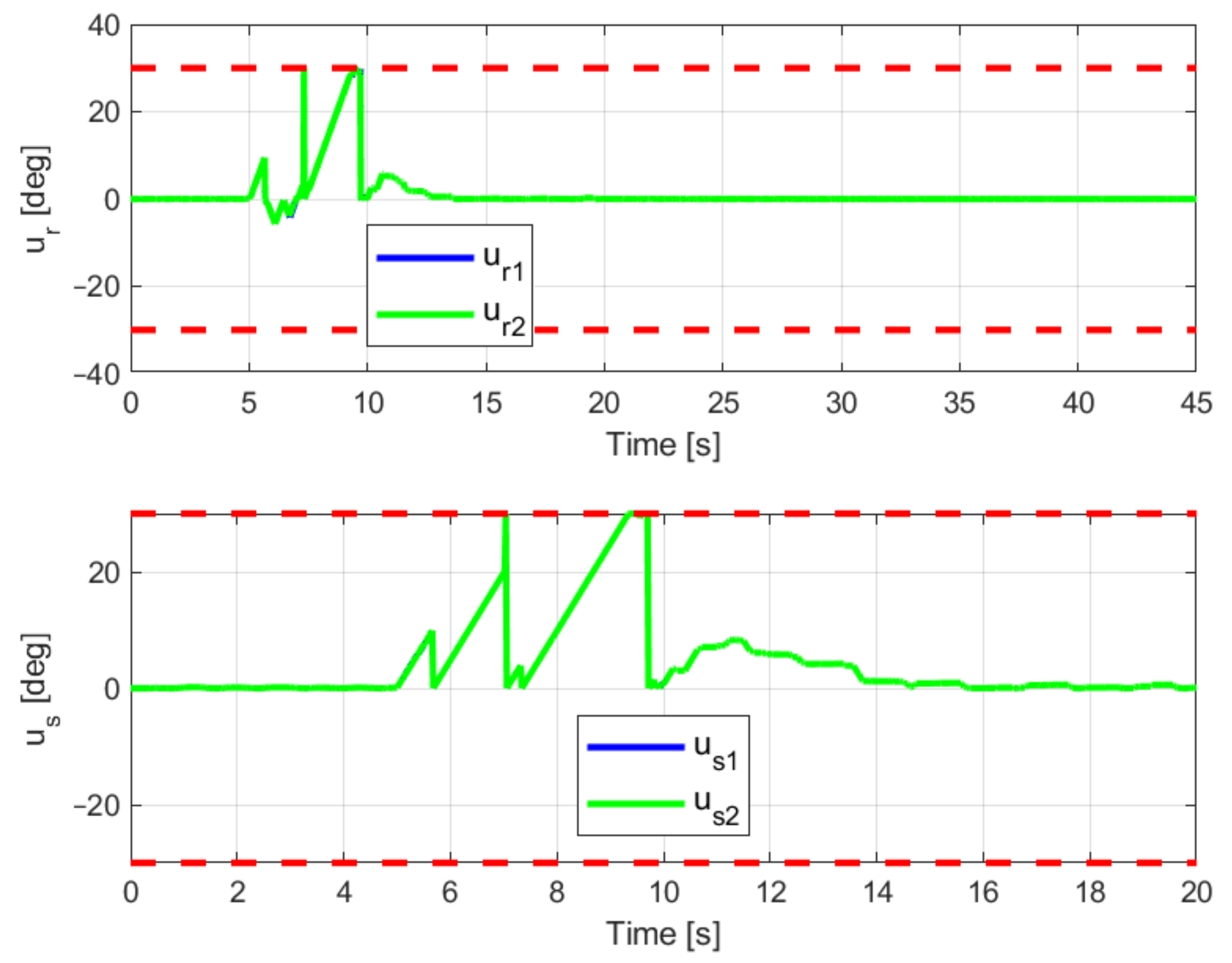
The fins are placed at the rear of the vehicle, near the main rear thruster. The dynamic response of the fins is directly related to vehicle pose and velocities, according to a set of relationships determined by the fins’ lift coefficients. The force and moment provided by the rudder fins ( Y r and N r ), stern planes ( Z s and M s ) and their combined effects ( K r s ) are:
Y r = 1 2 Y u u δ r u 2 0.5 δ r 1 + 0.5 δ r 2 + 1 2 Y u v f uv + 1 2 Y u r f ur
Z s = 1 2 Z u u δ s u 2 0.5 δ s 1 + 0.5 δ s 2 + 1 2 Z u w f uw + 1 2 Z u q f uq
K r s = 1 2 K u u δ r u 2 0.5 δ r 1 0.5 δ r 2 + 0.5 δ s 1 0.5 δ s 2
M s = 1 2 M u u δ s u 2 0.5 δ s 1 + 0.5 δ s 2 + 1 2 M u w uw + 1 2 M u q f uq
N r = 1 2 N uu δ r u 2 0.5 δ r 1 + 0.5 δ r 2 + 1 2 N uv uv + 1 2 N urf ur
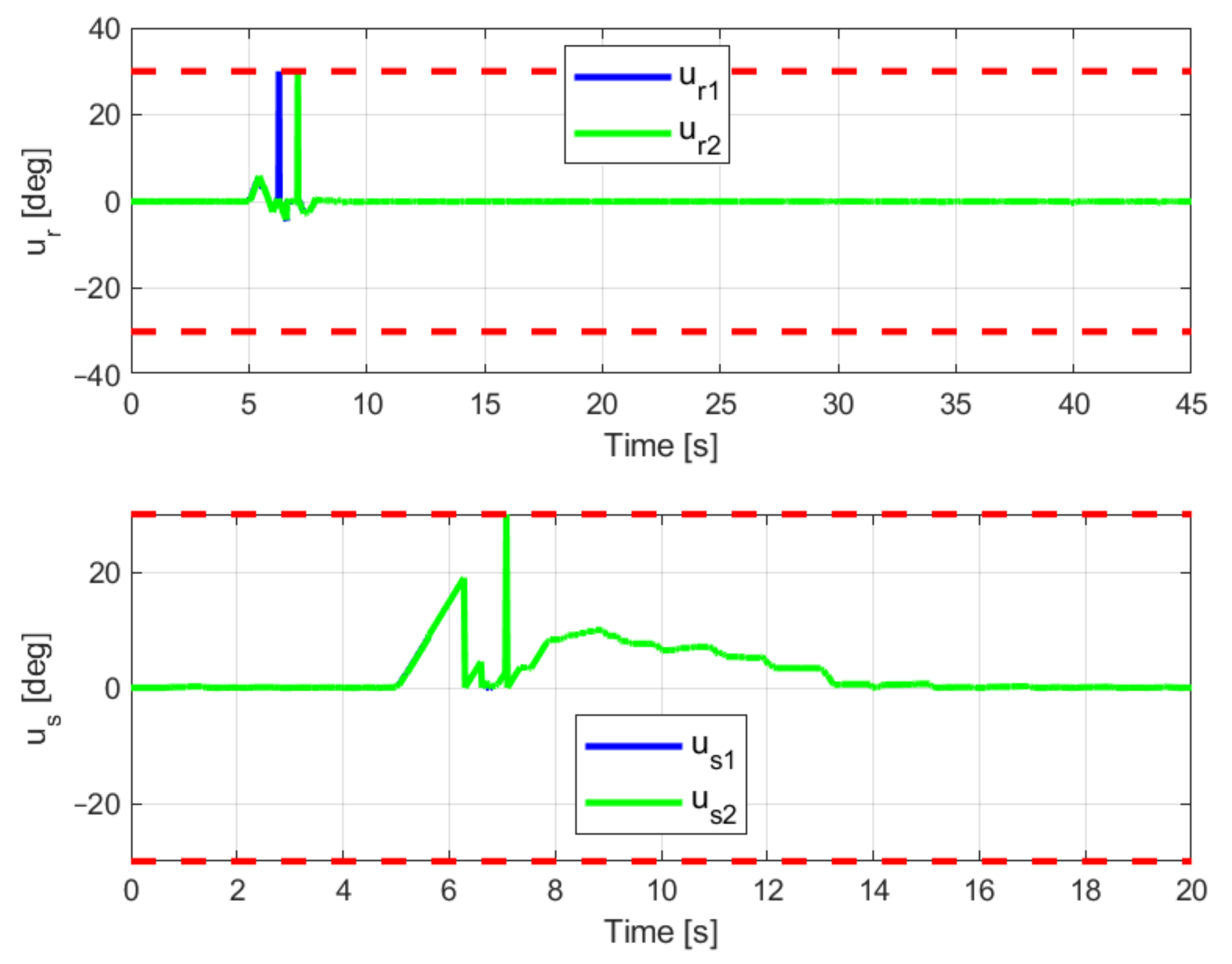
The control input for the fins is the deviation angle with respect to the zero position (in the body-fixed reference frame, δ r 1 , 2 and δ s 1 , 2 for rudders and stern-planes, respectively), and it is subject to saturation on maximum/minimum values (±30 degrees) according to the specifications provided. The dynamics of the fins’ angular position response, with respect to the reference provided by the control system, are represented by a second-order system with a natural frequency ω n = 4   H z and a damping factor ζ = 0.7 .
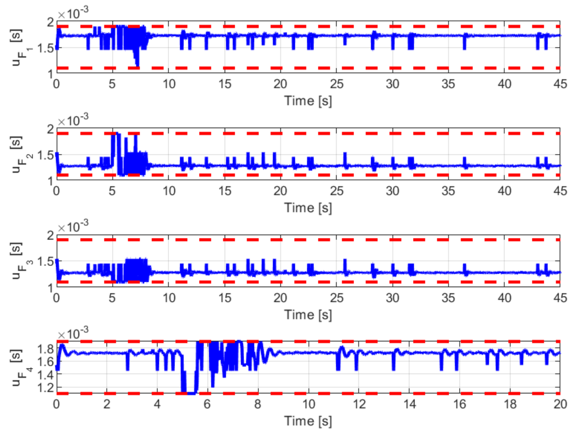
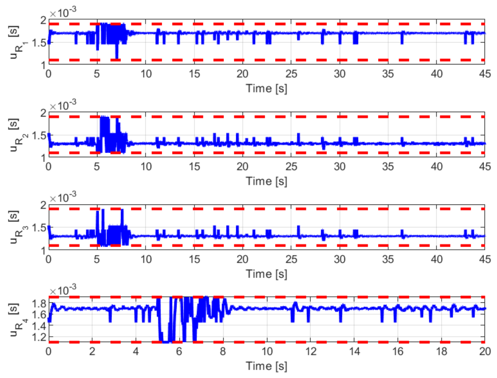
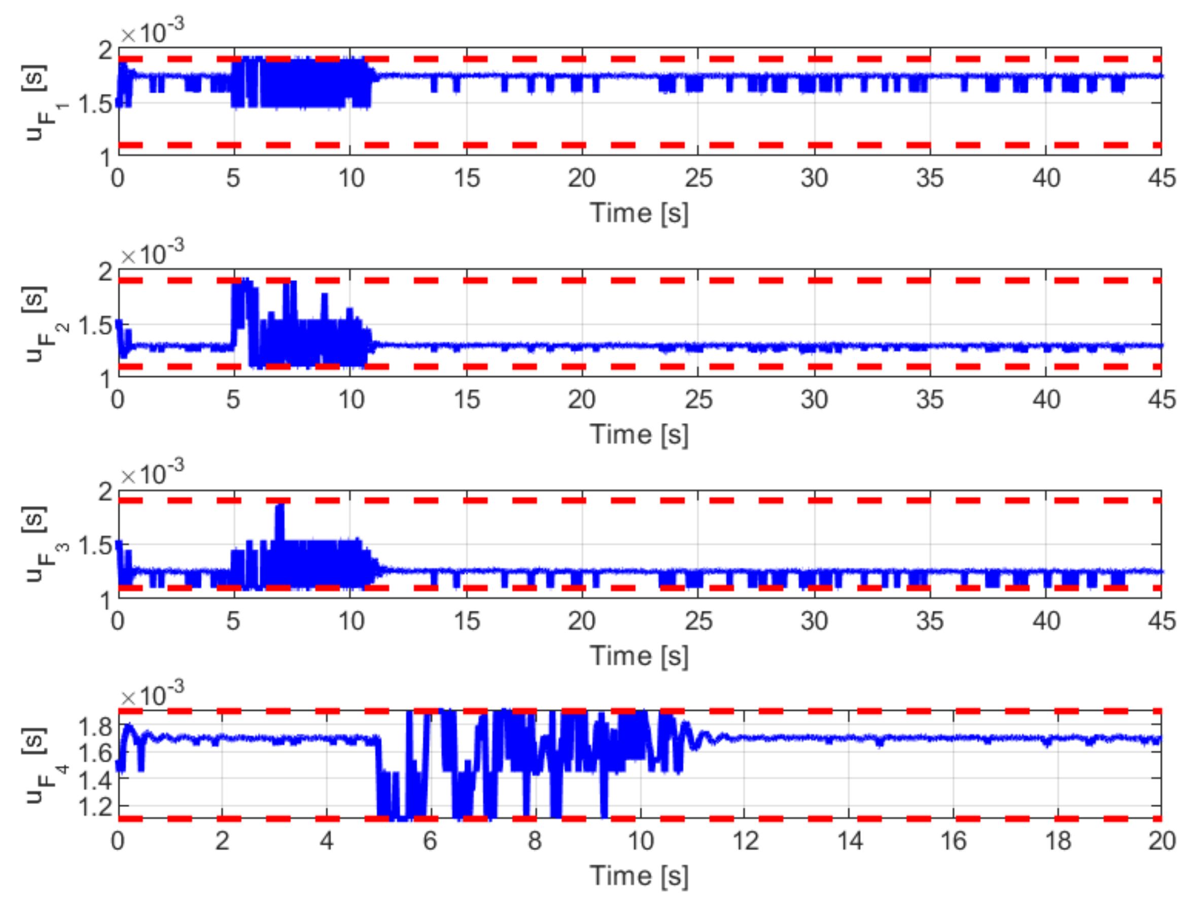
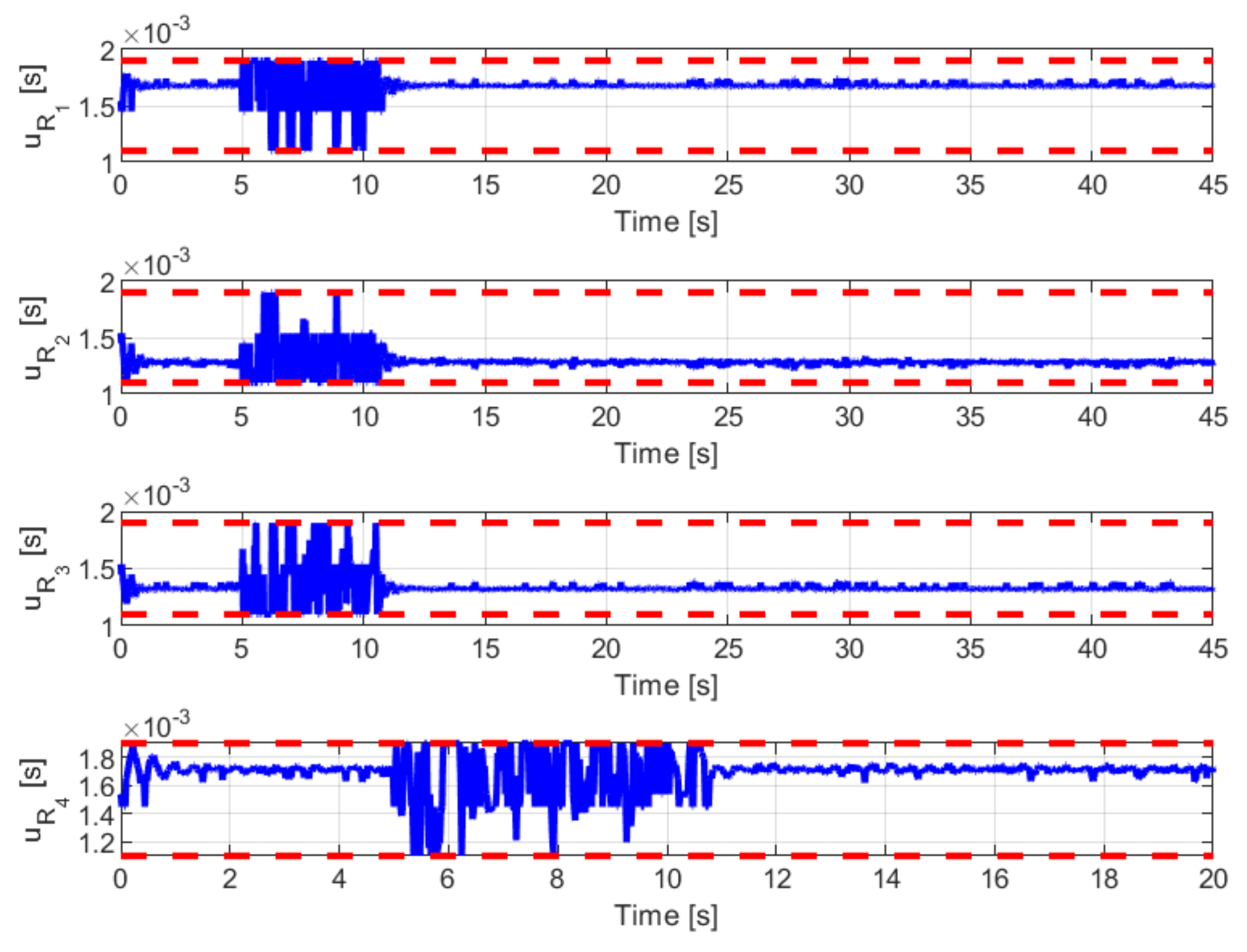
The side thrusters are placed on the side of the vehicle’s hull to drive the AUV at low speeds when the forward speed of the vehicle is too low for the fins to provide an effective control action. Because of the orientation of the thruster set, with respect to the body-fixed reference frame, the effort provided by each thruster can be split into two components. Given the position and the orientation of the thrusters, the combination of the thrusters’ effort may be modelled by the following relationships:
τ S T = 0 0 0 0 0 0 0 0 c α c α c α c α c α c α c α c α c α c α c α c α c α c α c α c α d d d d d d d d D F c α D F c α D F c α D F c α D R c α D R c α D R c α D R c α D F c α D F c α D F c α D F c α D R c α D R c α D R c α D R c α F F 1 F F 2 F F 3 F F 4 F R 1 F R 2 F R 3 F R 4
with τ S T = X S T ,   Y S T ,   Z S T ,   N S T ,   M S T ,   N S T T , where c α = cos α and α = 45 degrees is the angular position of thrusters (for α = 45 degrees sin α = cos α ), τ S T is the vector of forces and moments provided by the side thrusters in the body-fixed reference frame. The vector of forces provided by each thruster is computed according to the nonlinear characteristic of this actuator, converting the PWM duty-cycle (provided by the controller) to the thruster effort. These thrusters also include a saturation on the maximum force, and a symmetric dead-band cantered on the zero speed (equivalent to 1500 μs PWM input signal). The side thruster model is affected by a delay 0.01875 s and has the following dynamics model:
A T = 10 3 25 × 10 4 1 0 ;   B T = 1 0 ;   C T = 0 25 × 10 4
The thrust y T = T [N] provided by the actuator is defined in terms of the control input signal u T = P W M   m s and y T k = a 2 k u T 2 k + a 1 k u T k + a 0 k . The characteristic is defined by the following:
  • If u T k > 1.5381 then a 2 k = 54.262 , a 1 k = 108.231 and a 0 k = 38.101 ;
  • If u T k < 1.4492 then a 2 k = 28.058 , a 1 k = 134.08 and a 0 k = 135.38 ;
  • If u T k 1.4492 , 1.5381 then a 2 k = 0 , a 1 k = 0 and a 0 k = 0 .

Appendix B

In this appendix, the parameters are provided for the AUV nonlinear dynamics model in Appendix A. The model is a scale model of REMUS AUV presented in reference [15]. These parameters, used to describe the nonlinear system, are further used to define the control system algorithms (MPC, TA and KF). Table A1 collects the AUV hull vessel parameters, Table A2 reports the hydrodynamics damping coefficients, Table A3 provides the added mass coefficients, Table A4 lists the body lift coefficients and Table A5 gives the fin lift coefficients.
Table A1. AUV Hull Parameters.
AUV Model Parameters
ParameterSymbolValueUnit
Hull diameter b 0.324 m
Vehicle total length L 3.000 m
Vehicle buoyancy B 1999 N
Vehicle weight W 1940 N
Centre of buoyancy (CB) ( x c b , y c b , z c b )(−1.378,0,0) m
Moments of inertia, to CB( I x x , I y y , I z z )(5.8,114,114) k g · m 2
Table A2. AUV Hydrodynamic Damping Coefficients.
AUV Hydrodynamic Damping Coefficients
ParameterSymbolValueUnit
AUV axial drag X u u −12.7 k g / m
Crossflow drag coeff. Y v v −574 k g / m
Crossflow drag coeff. Z w w −574 k g / m
Crossflow drag coeff. Y r r d 12.3 k g · m / r a d 2
Crossflow drag coeff. Z q q d 12.3 k g · m / r a d 2
Crossflow drag coeff. M w w d 27.4 k g
Crossflow drag coeff. M q q −4127 k g · m 2 / r a d 2
Crossflow drag coeff. N v v d −27.4 k g
Crossflow drag coeff. N r r −4127 k g · m 2 / r a d 2
Rolling resistance coeff. K p p −0.63 k g · m 2 / r a d 2
Seawater density ρ 1024 k g / m 3
Gravity acceleration g 9.8 m / s 2
Table A3. AUV Added Mass Coefficients.
AUV Added Mass Coefficients
ParameterSymbolValueUnit
Added mass coeff. X u d −6 k g
Added mass coeff. Y v d −230 k g
Added mass coeff. Z w d −230 k g
Added mass coeff. K p d −1.31 k g · m 2 / r a d
Added mass coeff. M q d −161 k g · m 2 / r a d
Added mass coeff. N r d −161 k g · m 2 / r a d
Added mass coeff. Y r d 28.3 k g · m / r a d
Added mass coeff. Z q d −28.3 k g · m / r a d
Added mass coeff. M w d −28.3 k g · m
Added mass coeff. N v d 28.3 k g · m
Added mass coeff. X u d −6 k g
Added mass coeff. Y v d −230 k g
Table A4. AUV Body Lift Coefficients.
AUV Body Lift Coefficients
ParameterSymbolValueUnit
Body lift moment coeff. Y u v −82.3 k g / m
Body lift moment coeff. Z u w −82.3 k g / m
Body lift force coeff. M u w b −29 k g
Body lift force coeff. N u v b 29 k g
Table A5. AUV Fin Lift Coefficients.
AUV Fin Lift Coefficients
ParameterSymbolValueUnit
Fin lift coeff. Y u u δ r 27.7 k g / r a d · m
Fin lift coeff. Z u u δ s −27.7 k g / r a d · m
Fin lift coeff. M u u δ s −39.9 k g / r a d
Fin lift coeff. N u u δ r −39.9 k g / r a d
Fin lift coeff. Y u v f −27.7 k g / m
Fin lift coeff. Z u w f −27.7 k g / m
Fin lift coeff. Y u r f 17.7 k g / r a d
Fin lift coeff. Z u q f −17.7 k g / r a d
Fin lift coeff. M u w f −39.9 k g
Fin lift coeff. N u v f 39.9 k g
Fin lift coeff. K u u δ r 9.41 k g / r a d · m
Fin lift coeff. K u u δ s 9.41 k g / r a d · m

References

  1. Encarnacao, P.; Pascoal, A. 3D Path Following for Autonomous Underwater Vehicle. In Proceedings of the 39th IEEE Conference on Decision and Control, Sydney, Australia, 12–15 December 2000. [Google Scholar]
  2. Wei, Y.; Zhu, D.; Chu, Z. Underwater Dynamic Target Tracking of Autonomous Underwater Vehicle Based on MPC Algorithm. In Proceedings of the 2018 IEEE 8th International Conference on Underwater System Technology: Theory and Applications (USYS), Wuhan, China, 1–3 December 2018. [Google Scholar]
  3. Qiao, L.; Zhang, W. Fast Trajectory Tracking Control of Underactuated Autonomous Underwater Vehicles. In Proceedings of the 2018 IEEE 8th International Conference on Underwater System Technology: Theory and Applications (USYS), Wuhan, China, 1–3 December 2018. [Google Scholar]
  4. Uchihori, H.; Yamamoto, I.; Morinaga, A. Autonomous Underwater Vehicle Docking Concept Using 3D Imaging Sonar. Sens. Mater. 2019, 31, 4223–4230. [Google Scholar] [CrossRef]
  5. Chu, Z.; Zhu, D. Adaptive sliding mode heading control for autonomous underwater vehicle including actuator dynamics. In Proceedings of the OCEANS 2016, Shanghai, China, 19–22 September 2016. [Google Scholar]
  6. Gao, z.; Guo, g. Adaptive formation control of autonomous underwater vehicles with model uncertainties. Int J Adapt Control Signal Process. 2018, 32, 1067–1080. [Google Scholar] [CrossRef]
  7. Naeem, W.; Sutton, R.; Almad, M. Pure Pursuit Guidance and Model Predictive Control of an Autonomous Underwater Vehicle for Cable/Pipeline Tracking. In Proceedings of the Institute of Marine Engineering Science and Technology Part C Journal of Marine Science and Environment, San Francisco, CA, USA, 1 October 2003. [Google Scholar]
  8. Shen, C.; Shi, Y. Distributed implementation of nonlinear model predictive control for AUV trajectory tracking. Automatica 2020, 115, 108863. [Google Scholar] [CrossRef]
  9. Cavanini, L.; Ippoliti, G. Fault tolerant model predictive control for an over-actuated vessel. Ocean Eng. 2018, 160, 1–9. [Google Scholar] [CrossRef]
  10. Cavanini, L.; Cimini, G.; Ippoliti, G. Computationally efficient model predictive control for a class of linear parameter-varying systems. IET Control Theory Appl. 2018, 12, 1384–1392. [Google Scholar] [CrossRef]
  11. Cavanini, L.; Cimini, G.; Ippoliti, G. A fast model predictive control algorithm for linear parameter varying systems with right invertible input matrix. In Proceedings of the 2017 25th Mediterranean Conference on Control and Automation (MED), Valletta, Malta, 3–6 July 2017; pp. 42–47. [Google Scholar]
  12. Cavanini, L.; Cimini, G.; Ippoliti, G.; Bemporad, A. Model predictive control for pre-compensated voltage mode controlled DC–DC converters. IET Control Theory Appl. 2017, 11, 2514–2520. [Google Scholar] [CrossRef] [Green Version]
  13. Cha, S.H.; Rotkowitz, M.; Anderson, B.D. Gain Scheduling using Time-varying Kalman Filter for a class of LPV Systems. IFAC Proc. Vol. 2008, 41, 4934–4939. [Google Scholar]
  14. Antonelli, G.; Fossen, T.I.; Yoerger, D.R. Modeling and control of underwater robots. In Springer Handbook of Robotics; Springer: Cham, Switzerland, 2006. [Google Scholar] [CrossRef]
  15. Prestero, T. Verification of a Six-Degree of Freedom Simulation Model for the REMUS Autonomous Underwater Vehicle. Ph.D. Thesis, Massachusetts Institute of Technology, Cambridge, MA, USA, 2001. [Google Scholar]
  16. Grimble, M.J.; Majecki, P. Nonlinear Industrial Control Systems: Optimal Polynomial Systems and State-Space Approach; Springer: London, UK, 2020; ISBN 978-1-4471-7455-4. [Google Scholar]
Figure 1. AUV Conceptual Layout.
Applsci 11 04368 g001
Figure 2. AUV Control System Architecture.
Applsci 11 04368 g002
Figure 3. No current test: controlled variables (blue plot) with respect to the target position (dashed black plot).
Applsci 11 04368 g003
Figure 4. No current test: main thruster control signal (blue plot) with respect to the saturation and backlash values (dashed red plot).
Applsci 11 04368 g004
Figure 5. No current test: fins control signals (blue and green plot) with respect to the saturation values (dashed red plot).
Applsci 11 04368 g005
Figure 6. No current test: rear side thrusters’ control signals (blue plot) with respect to the saturation values (dashed red plot).
Applsci 11 04368 g006
Figure 7. No current test: rear side thrusters’ control signals (blue plot) with respect to the saturation values (dashed red plot).
Applsci 11 04368 g007
Figure 8. Max current test: controlled variables (blue plot) with respect to the target position (dashed black plot).
Applsci 11 04368 g008
Figure 9. Max current test: main thruster control signal (blue plot) with respect to the saturation and backslash values (dashed red plot).
Applsci 11 04368 g009
Figure 10. Max current test: fins control signals (blue and green plot) with respect to the saturation values (dashed red plot).
Applsci 11 04368 g010
Figure 11. Max current test: rear side thrusters’ control signals (blue plot) with respect to the saturation values (dashed red plot).
Applsci 11 04368 g011
Figure 12. Max current test: rear side thrusters’ control signals (blue plot) with respect to the saturation values (dashed red plot).
Applsci 11 04368 g012
Figure 13. “Naminow-D” docking technology demonstrator.
Applsci 11 04368 g013
Table 1. AUV Controller Tuning Parameters.
AUV Control System Tuning Parameters
ParameterSymbolValue
Prediction horizon N p 10
Control horizon N u 1
Control rate weights R 1 ,   1 ,   1 ,   0.1 ,   0.1 ,   0.1
Controlled output weights Q 0.1 ,   0.1 ,   0.1 ,   0.01 ,   0.01 ,   0.01
Terminal weights P 2 × 10 3 ,   3 × 10 7 ,   10 8 ,   10 7 ,   5 × 10 7 , 10 7
Publisher’s Note: MDPI stays neutral with regard to jurisdictional claims in published maps and institutional affiliations.

