
The Long-Term Consequences of Forest Fires on the Carbon Fluxes of a Tropical Forest in Africa


Helmholtz Centre for Environmental Research-UFZ Leipzig, Department of Ecological Modelling, Permoserstr. 15, 04318 Leipzig, Germany
Appl. Sci. 2021, 11(10), 4696; https://0-doi-org.brum.beds.ac.uk/10.3390/app11104696
Submission received: 4 May 2021
/
Revised: 18 May 2021
/
Accepted: 19 May 2021
/
Published: 20 May 2021
(This article belongs to the Special Issue Fires and Modelling for Succession in Forests)
Abstract
:Tropical forests are an important component of the global carbon cycle, as they store large amounts of carbon. In some tropical regions, the forests are increasingly influenced by disturbances such as fires, which lead to structural changes but also alter species composition, forest succession, and carbon balance. However, the long-term consequences on forest functioning are difficult to assess. The majority of all global forest fires are found in Africa. In this study, a forest model was extended by a fire model to investigate the long-term effects of forest fires on biomass, carbon fluxes, and species composition of tropical forests at Mt. Kilimanjaro (Tanzania). According to this modeling study, forest biomass was reduced by 46% by fires and even by 80% when fires reoccur. Forest regeneration lasted more than 100 years to recover to pre-fire state. Productivity and respiration were up to 4 times higher after the fire than before the fire, which was mainly due to pioneer species in the regeneration phase. Considering the full carbon balance of the regrowing forest, it takes more than 150 years to compensate for the carbon emissions caused by the forest fire. However, functional diversity increases after a fire, as fire-tolerant tree species and pioneer species dominate a fire-affected forest area and thus alter the forest succession. This study shows that forest models can be suitable tools to simulate the dynamics of tropical forests and to assess the long-term consequences of fires.
1. Introduction
Tropical forests are important for the climate of the Earth because they represent a relevant carbon sink [1,2,3]. Tropical forests account for about 50% of the total carbon stored in global vegetation [4,5]. However, these forests are threatened by various environmental and anthropogenic hazards such as logging and fire [6,7,8,9]. Between 2000 and 2012, tropical rainforests accounted for 32% of global forest area loss [10]. Extreme weather events and agricultural practices have already intensified forest fire regimes, which have led to accelerated losses of tropical forest [11,12]. Global fire carbon emissions were 2.0 Gt C per year (=109 t of carbon), with the majority of carbon emissions occurring in savannas and tropical forests [13]. Annual carbon emissions from tropical deforestation and degradation were on average 0.5 Gt C, whereby it is debated whether these carbon emissions from fires may not be compensated by forest regrowth after the fire [13]. It is also assumed that the number of fires in tropical forests will continue to increase in the future [14].
Almost 70% of all global forest fires are found in Africa [15,16]. These fires are rarely caused by natural processes such as lightning strikes; instead, human actions are often the cause [17]. This can happen through conversion to agricultural land but also through poachers or gatherers [17,18]. Forest fires can have an impact on the species composition, the living biomass, and the carbon balance of tropical forests [19].
These fires are also an influential ecological factor in the forests around Mt. Kilimanjaro in Africa [15,18,20]. In the last century, the impact of fire on the vegetation has increased due to climatic changes as well as the consequences of the growing population in the Kilimanjaro area. The upper tree line has already decreased by up to 800 m in altitude [15]. Consequently, about 15% of the forest area at the Kilimanjaro region has been destroyed in the last 40 years [15], with negative consequences for the water supply of lowland farmland.
However, the long-term consequences of fires on tropical forest dynamics are difficult to assess, as forest fires create heterogeneous landscapes with long-lasting impacts. A fire regime can be described by characteristics such as frequency, size, and severity. All these factors and also their interactions form a complex dynamic system. The long tradition in fire ecology has produced a broad understanding of these processes. Numerous models have been developed to simulate damages caused by fires in forests. These fire models are mainly developed as extensions of vegetation models [21,22,23]. Many fire models simulate the spread of fire as a function of topographic features. They were mainly developed for geoinformation systems and work on a scale of several kilometers [24]. Dynamic Global Vegetation Models (DGVM) have also been extended to include fire models [9,21]. Since these types of models mostly operate at a coarse scale of several kilometers, they use a top-down approach. Instead, high-resolution forest models operate at a much finer spatial resolution of up to 10–20 m [25,26]. In order to understand the effects of fire events on forest structure and dynamics, it is therefore necessary to develop an adapted fire model for this fine scale.
For the analysis of the effects of fire events on the dynamics of tropical forests at Mt. Kilimanjaro, the forest model FORMIND [27,28] was extended by a fire model. Specifically, the following question was answered: How strong is the influence of forest fires on the aboveground biomass, productivity, and carbon balance of sub-montane tropical forests at Mt. Kilimanjaro?
To answer this question, the forest model FORMIND was used to simulate typical fire patterns for this region and to look at long-term forest dynamics. For this purpose, first the forest dynamics after a fire event were investigated, i.e., the long-term regeneration of forest attributes such as biomass after the fire. In a second step, forest dynamics influenced by permanent recurrent forest fires were examined. To carry out this research, a new fire model was developed and integrated in the forest model.
2. Materials and Methods
2.1. Study Region Mt. Kilimanjaro
The tropical sub-montane forest area examined in this study is located within the forest belt at the base of Mt. Kilimanjaro (S 3.260150°, E 37.417458°; Figure 1). The climate is wet tropical with annual precipitation reaching 2.700 mm [29]. In this area, several forest research sites were established. Five forest sites (between 50 × 50 m and 100 × 100 m; in total 2 ha) were distributed along the southeastern slope of Mt. Kilimanjaro in the sub-montane and lower montane “Newtonia” rainforest (∼1150–2050 m a.s.l.). The dominant tree species are Heinsenia diervilleoides, Strombosia schefflera, Entandophrangma excelsum, and Garcinia tansaniensis. Forest inventories were conducted in each site in 2012 (by the German Research Foundation DFG within the Research Unit FOR1246) in cooperation with the Kilimanjaro National Park [30,31]. For this forest, a parameterization for the FORMIND forest model had already been developed and initial investigations about the carbon balance under natural conditions had been carried out [32,33].
2.2. The Forest Model FORMIND
FORMIND is an individual- and process-based forest model designed to simulate the dynamics of tropical forests [27,28]. For each tree in a stand, the processes of growth, mortality, and competition were calculated. Tree growth depends on a biomass balance, taking photosynthesis and respiration into account. At each time step (here: yearly), the biomass increment of each tree is calculated. Photosynthesis is derived on the basis of incoming radiation and shading by other trees. This forest model also includes a carbon module, which allows estimation of the full carbon balance of a forest stand, including the carbon fluxes in the soil and in the deadwood [34]. Hence, it is possible to determine the net ecosystem exchange (NEE), which is the difference between carbon uptake (i.e., photosynthesis) and carbon release (respiration and decomposition). The FORMIND model has already been used to study the carbon fluxes of tropical forests [34,35], and it is also able to simulate the effects of logging [36,37,38], but the simulation of forest fires is still missing.
A complete parameterization has already been created for the sub-montane forests at Mt. Kilimanjaro [32,33]. In addition, all occurring tree species have already been classified into six plant functional groups [32] (for an overview of the grouping, see Section 2.5 and Appendix A). In this study, no changes were made to the established parameterization.
2.3. Review of Fire Models
Here, three established fire models are reviewed, and the way in which their respective advantages can be used for a new fire model in FORMIND are discussed.
2.3.1. Fire Model by Drossel and Schwabl
The Drossel–Schwabl fire model is based on a cellular automaton [22,39]. A cell can be empty, covered with vegetation, or burning. The status of a cell change is rule-based: (1) An empty cell is populated with vegetation (here: tree) with probability p in the next step; (2) a cell with vegetation starts to burn with the inflammation rate f; (3) a cell with vegetation starts to burn if at least one neighboring cell is burning; (4) a burning cell becomes empty in the next step.
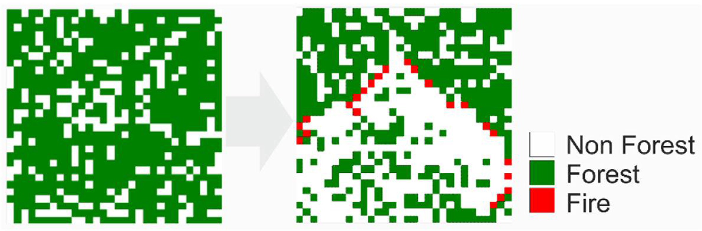
The main advantage of this fire model is the adequate modelling of the spread of fire, starting from the ignition source (Figure 2). However, the dynamical spread of fire events does not play a major role for this study. The disadvantage is the high computational effort (daily time step) and that each burning cell has completely no vegetation after the fire. In addition, it is not applicable for the individual-based forest model used, as it aggregates the complex forest structure into binary information of forest or non-forest.
2.3.2. Fire Model by Green
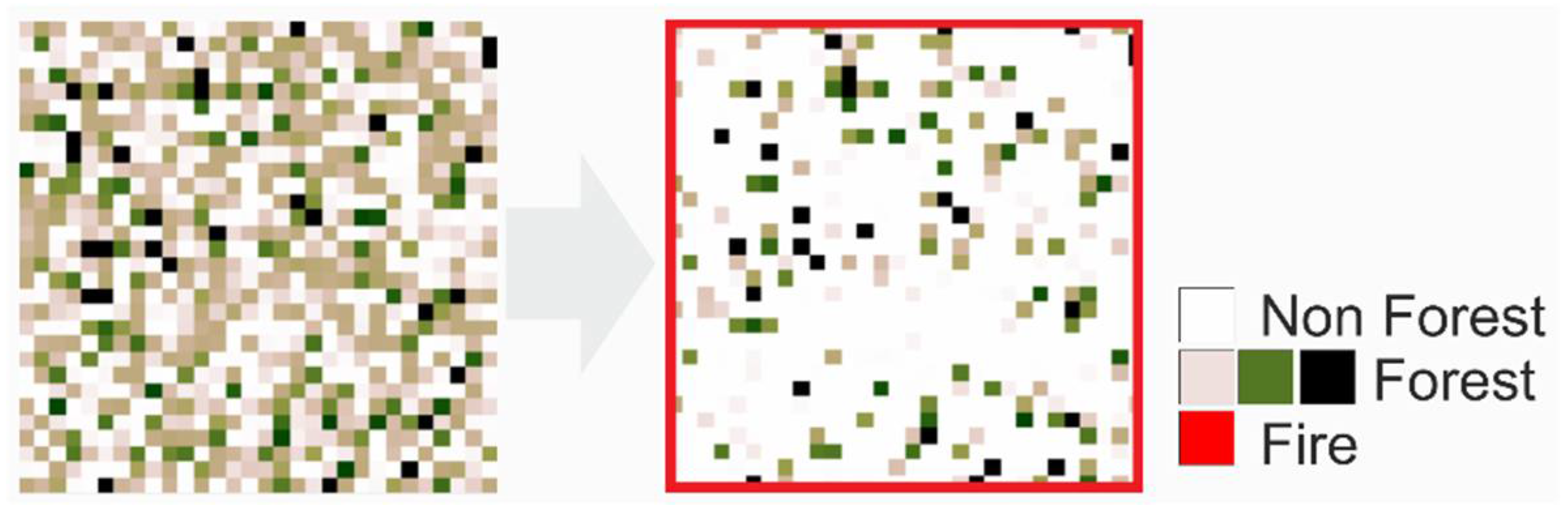
The landscape model MOSAIC was extended by a fire model [40]. This model is also based on a cellular automaton, where a cell consists of a single plant. Since fire events are rare events, they are described in this model with a Poisson process. If a fire breaks out, a randomly selected rectangular area burns (Figure 3). The size of the fire area is modelled as exponentially distributed. Once an area has burned down, it is immediately repopulated.
The strength of this model is the modelling of temporal dynamics between two fire events and the spatial variability in the fire affected area. The disadvantage is that all trees in the fire area always burn and die. In an extension of the model, this weakness was partially corrected by allowing only pioneer species to burn, while climax species survived [40].
2.3.3. Fire Model by Busing
To investigate the effects of fire on the forests of the USA, the forest model FORCLIM [41,42] was extended by a fire model [43,44]. The influence of fire on vegetation is modelled in such a way that fire-tolerant tree species have a greater probability of survival than fire-intolerant species, and larger trees survive more than smaller trees. The frequency of fire events but also the severity of a fire is realized randomly (Figure 4).
The disadvantage of this fire model is that there is always fire in the entire forest area. However, not all trees die, as this depends on the fire tolerance of the species and the size of the tree.
2.4. The New Fire Model ForFire
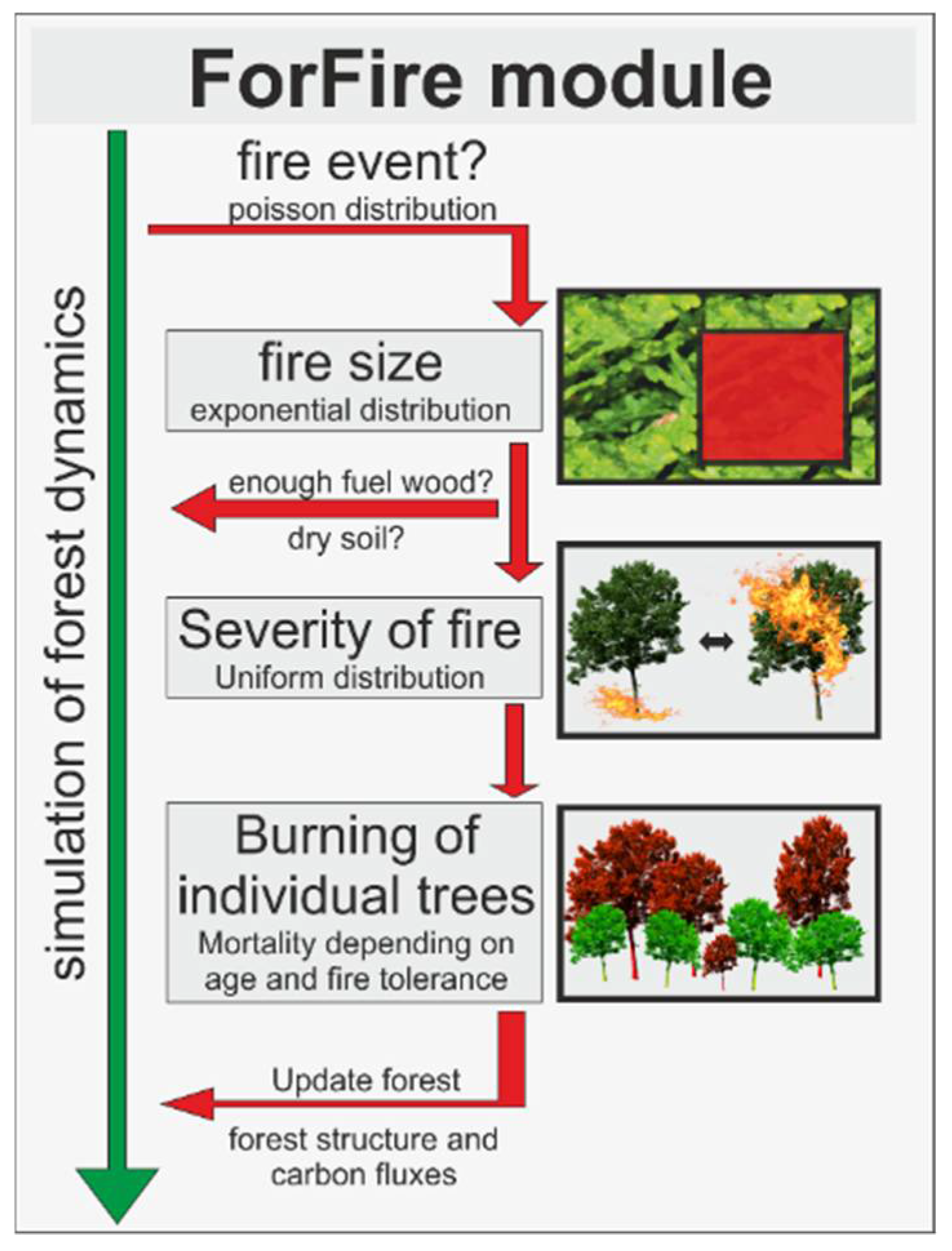
For the simulation of fire events with the individual-based forest model FORMIND, a separate fire model ForFire (Forest Fire model) was developed (Figure 5), which combines the advantages of the abovementioned fire models. The detailed dynamics of the fire spread are not relevant for this study, as the time step of the forest model is one year. For the fire model ForFire, it is important that the appearance of forest fires, the total spread of the fire area, and the generation of heterogeneous landscapes can be represented.
First, a stochastic process is introduced that counts the number of fires in a year (F in yr−1). This number of annual forest fires is assumed to be Poisson distributed:
where λ (yr) is the mean time interval between two fire events. If a fire breaks out in one year, the fire center is randomly determined on the entire simulated forest area. The size of the fire area (S in % of total forest area) is realized via an exponential distribution:
where β (%) is the relative size of the mean fire area with respect to the total simulated forest area. The area of the forest fire is chosen in such a way that, from a randomly chosen fire center, fire breaks out on randomly neighboring areas. This creates an irregular contiguous area around the fire center.
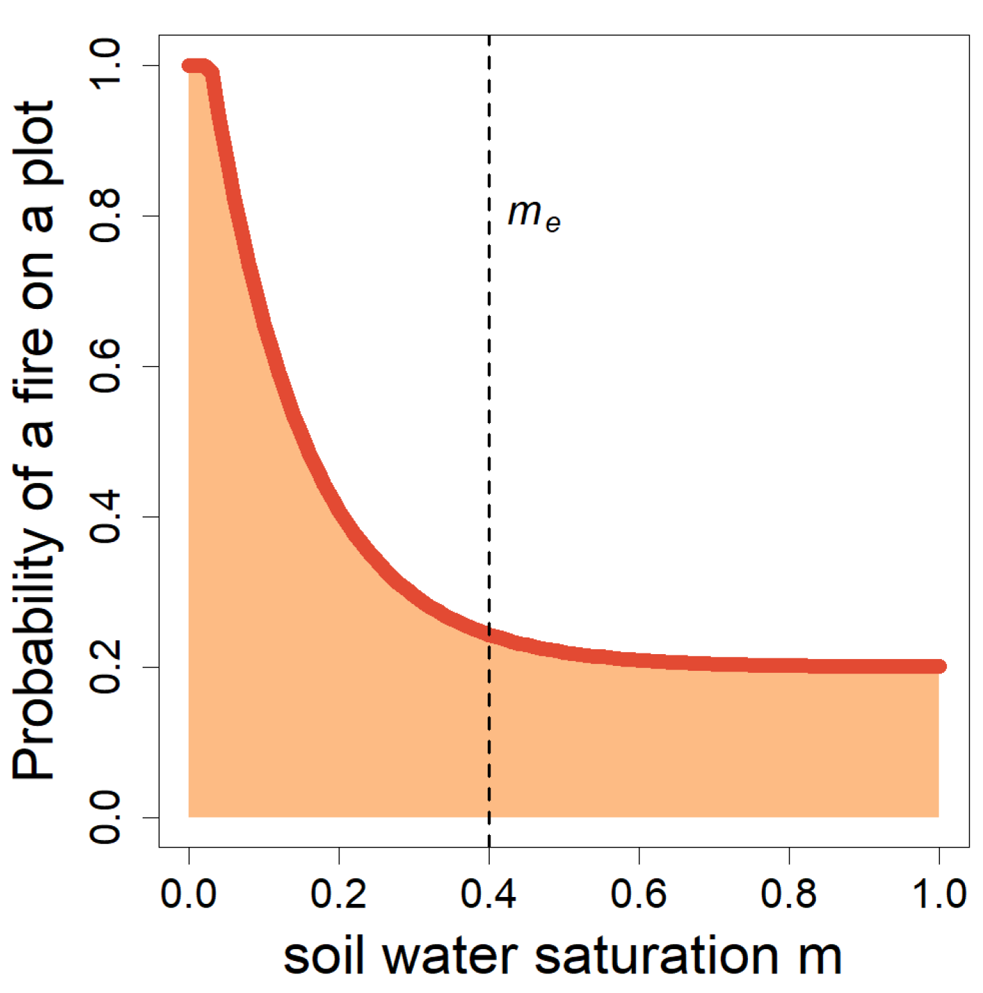
However, fire can only break out on a forest plot if there is enough flammable material. If there is less than 200 g/m2 of biomass in the area, the possibility for a fire to spread is almost non-existent [45]. In addition, the possibility of a fire breaking out is also dependent on climatic conditions, such as soil moisture, cf. SPITFIRE in LPJ [46]. This is integrated in the fire model ForFire by only starting a fire with a certain probability B on a plot within the fire area, depending on the soil water content (θ in Vol%) in the topsoil layer. For this purpose, the relative water saturation m (%) is calculated, which indicates how water-saturated the topsoil layer is [21]:
where MSW and Por are parameters of the soil [47]. For the ignition probability B (Figure 6) we get:
where me (%) is the saturation of the upper soil layer with water, above which it is very unlikely that a fire will start [21].
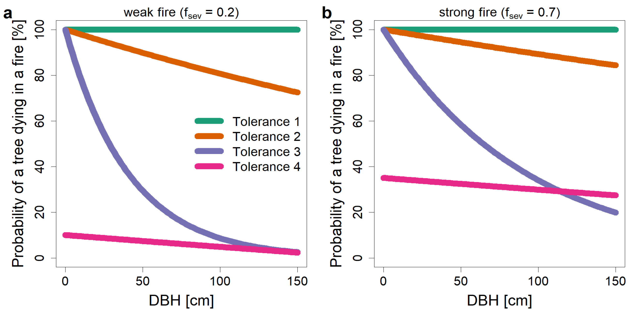
After determining the forest area in which the fire occurs, the next step considers all individual trees in the fire area. Every tree in the fire area is potentially at risk of burning and dying. The probability that a tree will burn depends on its species-specific fire tolerance and its trunk diameter [43]. Fire tolerance can be divided into four groups: Species with fire tolerance group 1 burn in any fire, whereas fire tolerance group 4 is very resistant to fire. The probability PFire that a tree with a stem diameter DBH [cm] will burn in a fire event is calculated according to [43] as follows, depending on the fire tolerance group (Figure 7):
where fsev (value 0–1) is an indicator of the severity and type of fire event. A ground fire (fsev ~ 0.2) is not as dangerous for the trees as a crown fire (fsev ~ 0.7). These probabilities were originally developed for the forest model CLIMACS, applied to forests in North America [48]. A distinction is made between tree species that always burn regardless of their size and the intensity of the fire event (fire tolerance group 1) and between tree species that have a certain probability of surviving a fire event if the trees are larger/older (fire tolerance group 2–4).
The described fire model ForFire combines the ideas of various established fire models. It has the advantages that the fire area changes spatially, that fire only breaks out under given vegetation conditions, and that trees only die with a certain probability, depending on a species-specific tolerance and the tree age (or stem diameter). The influence of a large forest fire on forest dynamics and carbon balance can be investigated, as well as the long-term consequences of recurrent fire events.
2.5. Simulation Settings
To analyze the effects of a fire event on forest dynamics, a forest area of nine hectares was simulated over a period of 500 years with a yearly time step. The fire model has four parameters: the mean fire frequency, the mean fire size, the mean fire intensity, and the fire tolerance of the individual species groups. To determine fire frequency in the study area, the satellite datasets “MODIS Burned Area Product MCD45” from 2000 to 2012 were analyzed. (In total 144 images were analyzed; see https://modis-fire.umd.edu/index.html, accessed on 12 February 2021, for more information about MODIS Burned Area Product; for user manual and downloading see https://modis-fire.umd.edu/files/MODIS_Burned_Area_Collection51_User_Guide_3.1.0.pdf, accessed on 12 February 2021). These maps show the monthly burned area in an area through spectral variations and changes in vegetation (see, for example, [49]). In the savannah area of the Kilimanjaro region, almost every year a fire can be observed; in the tropical forests of this region, a fire can be observed somewhat less frequently [15]. The analysis of the available satellite data for the entire Kilimanjaro area (region investigated: 2°29–3°72 South and 37°12–37°57 East) showed that a large-scale fire occurs on average every three to four years and is between 1 and 16 pixels in size (pixel resolution 500 m) [50]. The larger fires were observed in 2001, 2004, 2007, and 2009, and they mostly occur in the dry seasons, which are characterized by the El Nino Southern Oscillation [20].
In the forested area at Mt. Kilimanjaro, the satellite data show that on average a fire is about 25 hectares in size (=1 image pixel, with the size of 500 × 500 m). However, smaller fire areas cannot be detected due to the spatial resolution (i.e., 500 m) of the satellite product, and thus this mean size seems too high. Since the simulated forest area in the model has a size of 9 hectares, the mean fire area was set to 20% of the considered forest area—which corresponds to experiences from other areas [7,40,51]. Fire intensity indicates the difference between a light ground fire (fire intensity = 0.1) and a strong crown fire (fire intensity = 1.0). For this study, a mean value of 0.55 was set [43,48]. All parameter values for the fire model ForFire can be found in Table 1.
The mortality of a tree in a fire event is influenced by its fire tolerance. There are four groups of fire tolerance in the fire model: Species with fire tolerance group 1 burn in any fire, whereas fire tolerance group 4 is very resistant to fire. For each tree species in the study area, the fire tolerance was determined by the literature or expert knowledge (for a complete list, see Appendix A). The thickness of the bark is the most important factor [52]. The thicker a bark is, the less heat is generated in the cambium layer of the tree (responsible for the growth of the tree). In the study area, for example, the species Agarstia salicifolia and Morella salicifolia have particularly thick bark and are therefore considered to be fire tolerant [15,53,54]. The species Alagium chinense is a deciduous species, which is also considered to be adapted to the occurrence of fire [53,55]. The three fire-tolerant species mentioned belong to plant functional type 4. This species group was thus classified as fire tolerant (i.e., fire tolerance 4). The species Ilex mitis, on the other hand, is considered fire intolerant, as all trees of this species died in a fire experiment [56]. This species belongs to plant functional type 2, which was thus classified as fire intolerant (i.e., fire tolerance 1). Fire tolerance was determined for each plant functional type, depending on the fire tolerance of the individual tree species in the corresponding species group (Table 2, Appendix A).
3. Results
3.1. The Consequences of a Fire Event on the Carbon Fluxes in a Tropical Forest
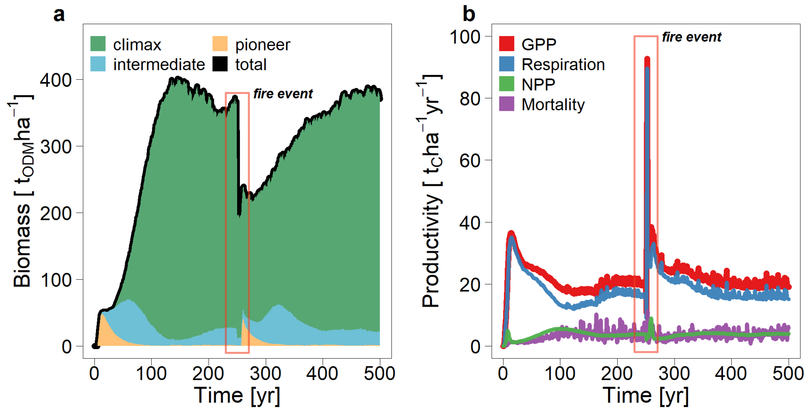
In order to understand the effects of a large-scale fire on tropical forest dynamics, a single fire was simulated with the forest model FORMIND (simulation area 9 ha, fire size 60%, fire severity 0.67; see Figure 8). After the simulated fire event, the total aboveground biomass was reduced by 46% (Figure 9). Overall, it takes up to 150 years after the fire event for the forest biomass to reach the level of an undisturbed forest and to stabilize—which is much longer than the natural succession (100 years, cf. Figure 9). Compared with the succession in the undisturbed forest, this is mainly due to the climax species, which need up to 2 times longer to reach the biomass level of the undisturbed forest.
Due to the different fire tolerances, but also due to the different tree size distributions of the individual tree species, the fire affects the species groups differently (Figure 9a). The biomass of the dominant climax species was reduced by 46%; the biomass of the pioneer species was reduced by about 53%. However, since the forest was dominated by climax species before the forest fire, this led to the largest absolute biomass losses (−158 t/ha) compared with the other species groups. After the fire, secondary succession starts at the burnt areas. First, the pioneer species colonize these areas. The previously absent fire-tolerant and shade-intolerant tree species dominate the forest in this regeneration phase. After about 50 years, the biomass of trees with high shade tolerance then also increases again.
Forest productivity two years after the fire is up to 4 times larger than before the fire (up to 92 tC/(ha yr), Figure 9b). The higher productivity is mainly caused by growing pioneer species on the burnt area. The respiration of the living vegetation increases 5-fold after the forest fire. However, the resulting net primary production remains rather stable after the fire at the value of about 3–4 tC/(ha yr). Both productivity and respiration do not return to pre-fire levels until more than 100 years after the fire (Figure 9b). Biomass loss due to mortality is very high during the fire, but already 10 years after the fire it almost reaches the level of 3.5 tC per hectare and year again (Figure 9b).
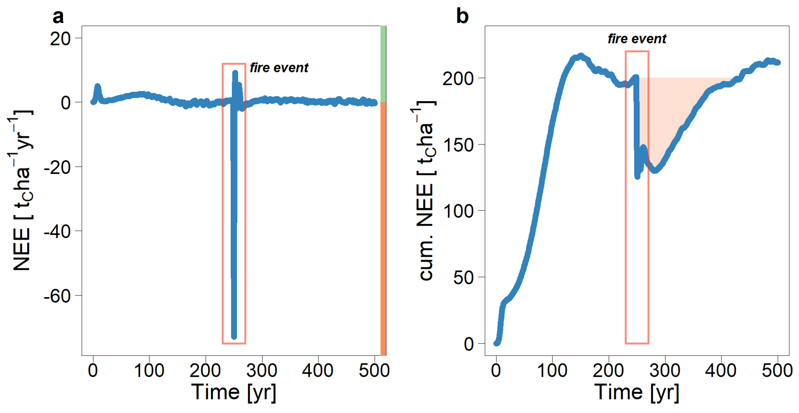
During the fire event, a negative carbon balance (NEE) was observed, as up to 75 tons of carbon per hectare are emitted (Figure 10a). In the ten years after the fire, the NEE was positive due to the high productivity of pioneer species. However, for the next 20 years, the carbon balance was negative, with an average annual carbon source of 0.8 tC/ha. In the following 50 years, the forest absorbs more carbon than it emits, on average 0.6 tC/ha per year. For the cumulative carbon balance, including the carbon emission released during the fire, the forest needs many decades to sequester enough carbon to return to pre-fire levels. The overall balance of the carbon fluxes remains negative for more than 150 years after the fire (Figure 10b).
3.2. The Influence of Recurrent Fire Events on Forest Dynamics
In order to estimate the consequences of regularly occurring fire events on the forest dynamics, numerous fires were simulated with the forest model FORMIND. On average, a fire of the size of 20% of the simulation area (9 hectares) was simulated every 4 years (cf. Table 1). This scenario corresponds to results of satellite data analysis on fire areas at the Kilimanjaro region.
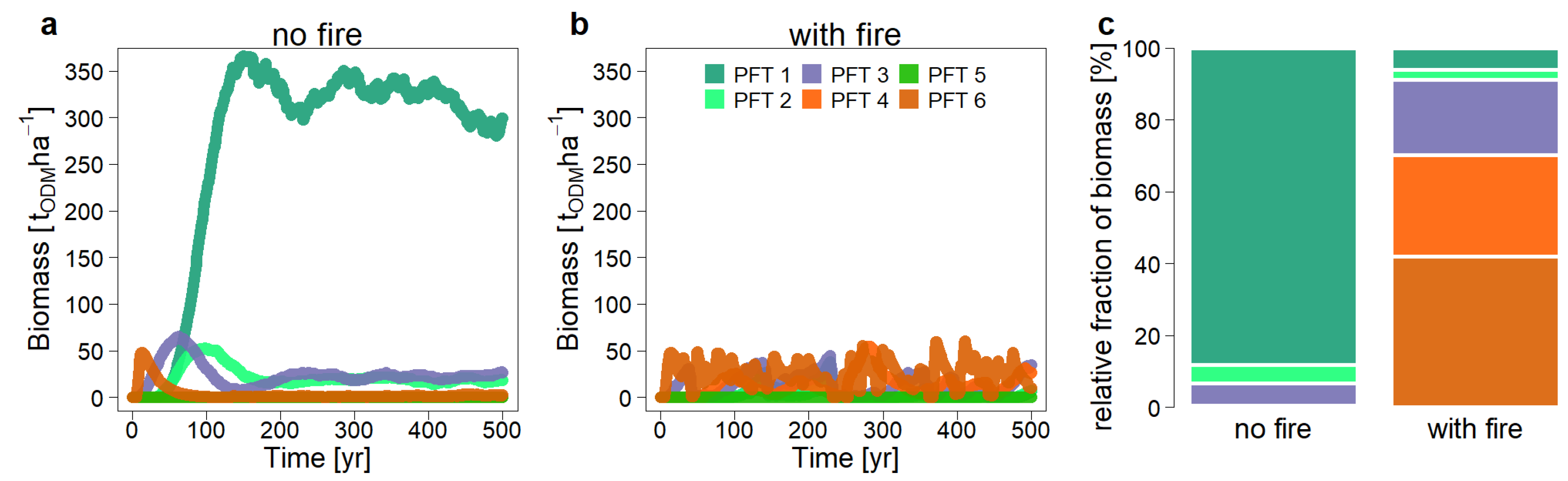
Compared with the undisturbed scenario without fire, the dynamics in the fire-disturbed forest are significantly altered (Figure 11). Total aboveground biomass is reduced by 80%; the forest thus has a deficit of 300 tons of biomass per hectare. The first species group consisting of large climax species has the largest reduction, as this species group loses 95% of its biomass. The pioneer species (PFT 4 and 6), on the other hand, can increase their biomass considerably. Both species groups account in total for 70% of the total biomass in the fire scenario, whereas they played no role in the undisturbed scenario. The disturbed forest does not reach a state of equilibrium in terms of species composition. The climax species can increase in biomass after a fire, but it loses a lot of biomass during the next fire event. Overall, the shade-tolerant tree species (PFT1 and 2) account for only 8% of the total biomass, which varies largely over time (1–45%).
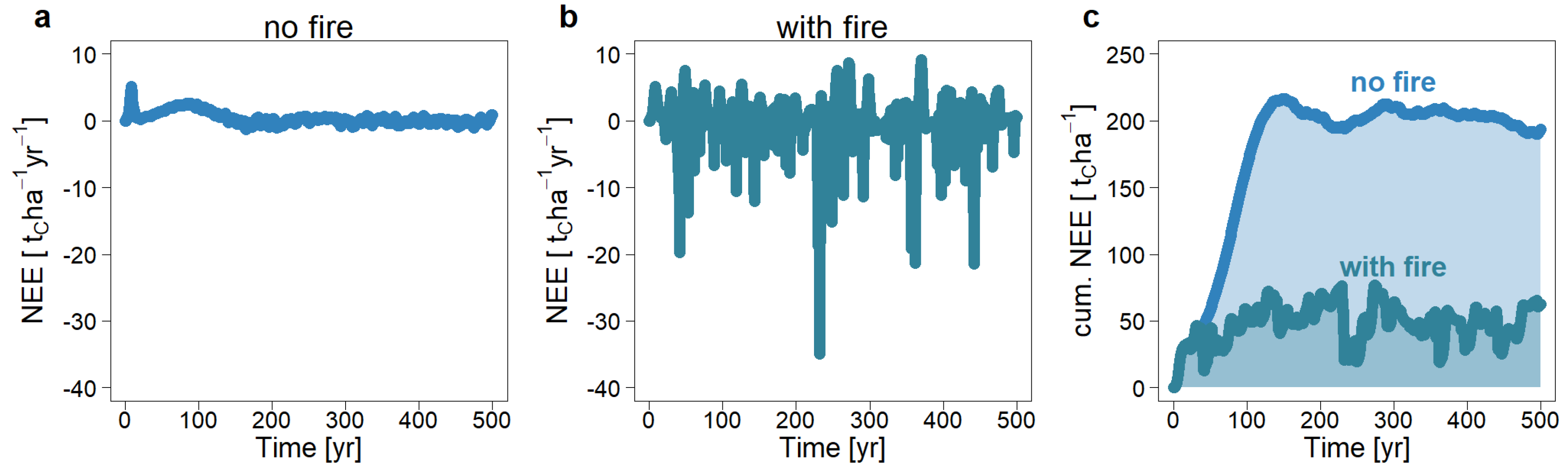
Due to the high carbon emissions during a fire event and the carbon sequestration in the regeneration phase after a fire, the variation of the carbon balance (NEE) is very high (Figure 12b). In the undisturbed forest, the standard deviation of carbon flux is 0.4 tC ha−1 yr−1, whereas in the scenario with regular forest fires, the standard deviation is 10 times higher. However, the mean carbon flux is balanced at zero, just as in the undisturbed scenario (Figure 12a,b). Considering the cumulative carbon balance of both scenarios (Figure 12c), both reach a state of equilibrium after about 100–150 years. However, the equilibrium state in the scenario without fire is 150 tC ha−1 higher.
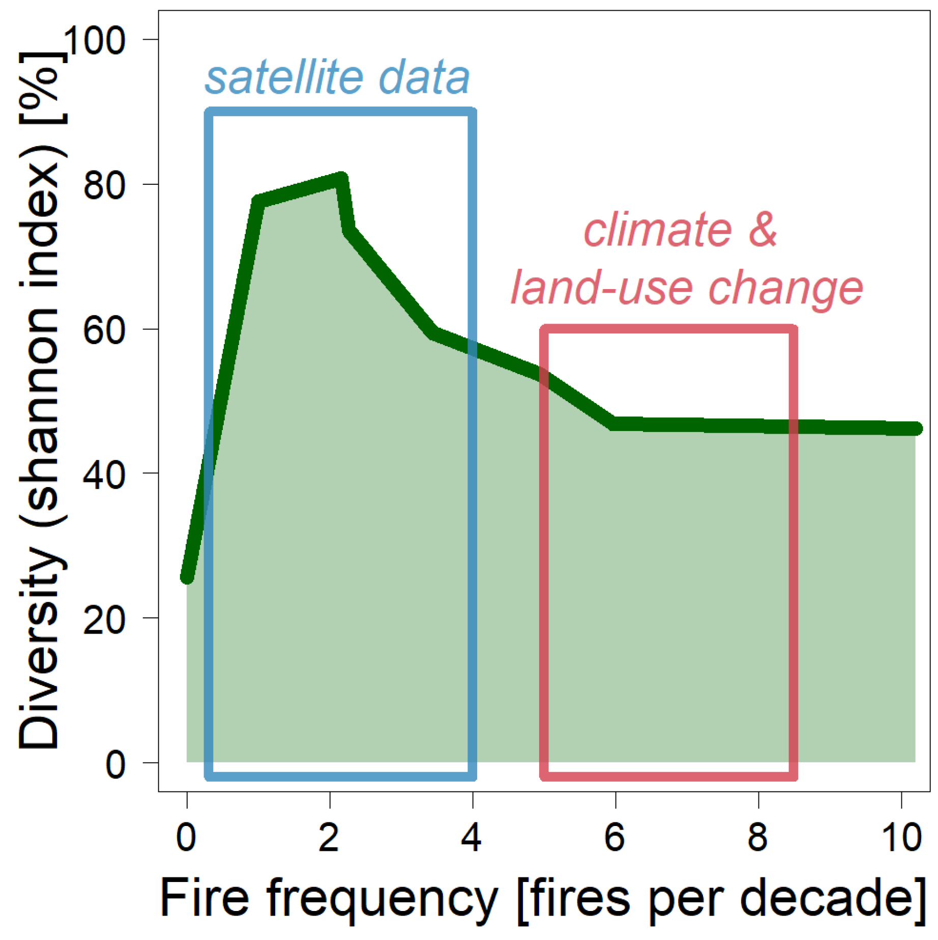
Investigating the species composition with increasing fire intensity, the simulation results show the typical picture of a hump-shaped curve (Figure 13). If the ecosystem is undisturbed (i.e., fire frequency is zero), the normalized Shannon Index is low at 30% (= standard Shannon Index divided by ln(6)). If a fire occurs annually (equivalent to 10 fires per decade), the Shannon Index increases to 50%. Fires that occur less frequently than annually, however, produce an even higher species diversity (Figure 13). This results in a maximum of the Shannon Index for 2–3 fire events per decade. Analysis of satellite data for the Kilimanjaro region showed between one to four forest fires per decade. Thus, high species diversity can be expected in disturbed areas around Mt. Kilimanjaro. If future fire frequency increases due to higher temperatures and less precipitation [14,57], there might be a reduction in functional diversity in the study area, according to the simulation results (Figure 13).
4. Discussion
Fires represent an important disturbance type when considering the terrestrial biosphere [14,57,58]. In a forest, fire can lead to strong changes, especially in species composition, forest succession, and carbon dynamics [19]. As African forests in particular are strongly affected by fire, it is important to study the different consequences of fire, as this can have an impact on forest dynamics, as well as on the function of tropical forests as a carbon sink. Two different scenarios were investigated in this modelling study. The first scenario analyzed the changes in aboveground biomass, productivity, and carbon balance of a tropical forest at Mt. Kilimanjaro after a large-scale fire. A second scenario analyzed changes after regularly recurring fires. It turned out that the forest needs more than 100 years to recover to its pre-fire state. The climax species lose the largest amount of biomass, as they dominated the forest before the fire. Productivity and respiration are up to 4 times higher after the fire than before the fire. This is mainly due to the regrowing pioneer species. After the fire, trees of fire-tolerant species will dominate a forest stand. This alters the succession in tropical forest, as it is more species-rich after a fire and the fire-tolerant species prolong the succession. This effect also has an influence on the carbon balance in a tropical forest. Please note that the results presented apply specifically to the parameterized forest area at the Mt. Kilimanjaro region. In addition, both the parameters of the forest model and the parameters of the fire model include uncertainties. Although monthly satellite data were available, it is challenging to make statements about the type of fire (ground fire vs. crown fire) and the area of spread.
Important in the analysis of the fire model was the consideration of the feedback of a fire event with the vegetation. This means that a fire has an influence on the vegetation, and the vegetation influences the characteristics of a fire. This was implemented in such a way that a fire only breaks out if combustible material is present and the soil or litter layer is relatively dry. Furthermore, a tree burns depending on its fire tolerance and its age. What is not considered are the long-term effects of fire on soil properties, such as nutrient inputs. Since the growth of trees in the forest model has so far been described independent of the nutrient balance in the soil, nutrient inputs have not been considered in this study.
In fact, no real fire experiment was conducted in the study area at Mt. Kilimanjaro. The fire experiments available in the literature often refer to the effects on grasslands [59,60,61]. These experiments involve little cost, the time horizon is manageable, and the damage to nature is not so high (compared to a fire experiment in a forest). Experiments concerning forest fires refer mostly to temperate forests or to the tropical forest in the Amazon. The influence of fire on forest structure, biomass, and species composition was investigated in such an experiment [7,62]. Losses in living biomass after fire ranged from 10% to 90%, depending on how often fire occurred in the area studied. Our simulations indicate that aboveground biomass can be reduced by between 40% and 80%, and thus the results are comparable to the analyses in the Amazon. This is also confirmed by a second study in the Amazon, which found 42% to 57% losses in biomass after a fire [63].
Some studies related to fire consider not only the loss of biomass but also the change in species composition [64,65]. In this simulation study, a significant change in species composition was also observed. The forest without disturbance was dominated by climax species; in the simulated forest with fire, the proportion of pioneer species increased. Thus, the species composition looked much more diverse. This was evaluated by calculating the normalized Shannon Index: in the undisturbed forest it was 30%, and in the fire-disturbed forest (fire events every 4 years), it reaches up to 80%. This means that fire events can increase functional diversity.
In this study the relationship between fire frequency and species diversity was also investigated, which is also a topic of the intermediate disturbance hypothesis (IDH) [66]: “The highest diversity of tropical rainforest trees should occur…with smaller disturbances that are neither very frequent nor infrequent”. According to this theory, ecosystems respond to light but regular disturbances with increasing species diversity. Species diversity shows a maximum at medium disturbance intensity. According to the IDH, however, species diversity declines again when disturbances are intense. This study shows a maximum of species diversity when 2–3 forest fires per decade occur in a region. Empirical studies in a forest-grassland ecotone showed similar results with a maximum of heterogeneity at five fire events per decade [65].
This simulation study at Mt. Kilimanjaro revealed that the investigated forest shows responses to disturbances similar to the IDH. Physiological trade-offs between different tree species—here the trade-off between growth and mortality—might be an important factor for this phenomenon. However, it must also be noted that with 2–3 fires per decade, the tropical forest has a much lower biomass level than an undisturbed forest, with negative consequences for its carbon balance.
5. Conclusions
Fires affect millions of hectares of tropical forest, generating billions of USD in damage annually [14]. Science should pay more attention to fire events in all tropical areas. This should not be done by simply transferring knowledge from fire experiments of temperate forests to the species-rich complex tropical forests. Instead, studies and experiments on the effects of forest fires in tropical areas should be intensified. This modelling study shows how a forest model can support such studies by extrapolating local findings in both time and space.
Funding
This study was conducted within the framework of the research unit FOR1246 (Kilimanjaro ecosystems under global change: linking biodiversity, biotic interactions and biogeochemical ecosystem processes) funded by the Deutsche Forschungsgemeinschaft (DFG). I acknowledge funding from the Helmholtz Alliance “Remote Sensing and Earth System Dynamics”.
Data Availability Statement
The forest model FORMIND, the source code, and the parametrization are freely available and can be downloaded from www.formind.org, 19 May 2021.
Acknowledgments
I want to thank Andreas Huth for helpful discussions and constructive comments on the manuscript and Ulrike Hiltner and Martina Alrutz for initial investigations of burned areas with satellite data. I would like to thank the reviewers for their thoughtful comments and efforts towards improving the manuscript.
Conflicts of Interest
The author declares no conflict of interest.
Appendix A
Species List of the Study Area at Mt. Kilimanjaro
List of tree species found in the tropical forest at Mt. Kilimanjaro with maximum growth height and light requirement (tol = shade tolerant; intol = shade intolerant; med = medium light requirement). All tree species were grouped into six plant functional types (PFT). For details of the species grouping, see [32,33]. In addition, the fire tolerance is indicated for each species (1 = fire intolerant to 4 = fire tolerant).
| Species | Max. Height (m) | Shade Tolerance | PFT | Fire Tolerance |
| Agarista salicifolia | 20 | intol | 4 | 4 |
| Alangium chinense | 25 | intol | 4 | 1 |
| Albizia gummifera | 30 | tol | 2 | 1 |
| Aningeria adolfi friedericii | 50 | tol | 1 | 1 |
| Aphloia theiformis | 15 | med | 3 | 1 |
| Bersama abyssinica | 20 | med | 3 | 1 |
| Canthium oligocarpum ssp captum | 10 | tol | 5 | 1 |
| Casearia battiscombei | 30 | tol | 1 | 1 |
| Celtis durandii | 25 | med | 3 | 1 |
| Clausena anisata | 20 | med | 3 | 1 |
| Cornus volkensii | 30 | med | 3 | 1 |
| Cyathea manniana | 15 | intol | 6 | 1 |
| Dracaena afromontana | 10 | tol | 5 | 1 |
| Dracaena laxissima | 5 | tol | 5 | 1 |
| Eckebergia capensis | 25 | tol | 2 | 1 |
| Embelia schimperi | 30 | tol | 2 | 1 |
| Entandrophragma excelsum | 70 | tol | 1 | 1 |
| Erica excelsa | 28 | intol | 4 | 4 |
| Erythrococca polyandra | 10 | tol | 5 | 1 |
| Ficus sur | 25 | med | 3 | 1 |
| Galiniera saxifraga | 15 | tol | 5 | 1 |
| Garcinia tansaniensis | 40 | tol | 1 | 1 |
| Garcinia volkensii | 20 | tol | 2 | 1 |
| Hagenia abyssinica | 25 | intol | 4 | 3 |
| Hallea rubrostipulata | 33 | med | 3 | 1 |
| Heinsenia diervilleoides | 25 | tol | 2 | 1 |
| Ilex mitis | 30 | tol | 2 | 1 |
| Lasianthus kilinandscharicus | 10 | tol | 5 | 1 |
| Lepidotrichilia volkensii | 16 | med | 3 | 1 |
| Leptonychia usambarensis | 15 | tol | 5 | 1 |
| Macaranga capensis var kilimandscharica | 30 | med | 3 | 1 |
| Maesa lanceolata | 20 | intol | 4 | 1 |
| Maytenus acuminata | 15 | tol | 5 | 1 |
| Morella salicifolia | 15 | intol | 4 | 4 |
| Myrica salicifolia | 15 | intol | 4 | 4 |
| Newtonia buchananii | 40 | tol | 1 | 1 |
| Ocotea usambarensis | 45 | tol | 1 | 2 |
| Olinia rochetiana | 25 | med | 3 | 1 |
| Pauridiantha paucinervis | 10 | tol | 5 | 1 |
| Pavetta abyssinica | 15 | tol | 5 | 1 |
| Peddiea fischeri | 15 | tol | 5 | 1 |
| Pittosporum spec lanatum | 10 | med | 3 | 1 |
| Podocarpus latifolius | 35 | tol | 1 | 1 |
| Polyscias fulva | 25 | intol | 4 | 1 |
| Polyscias albersiana | 15 | intol | 4 | 1 |
| Psychotria cyathicalyx | 15 | tol | 5 | 1 |
| Rapanea melanophloeos | 30 | med | 3 | 1 |
| Rawsonia lucida | 25 | tol | 2 | 1 |
| Rothmannia urcelliformis | 10 | tol | 2 | 1 |
| Schefflera myriantha | 30 | tol | 2 | 1 |
| Schefflera volkensii | 25 | tol | 2 | 1 |
| Strombosia scheffleri | 35 | tol | 1 | 1 |
| Syzygium guineense | 30 | tol | 2 | 1 |
| Tabernaemontana stapfiana | 25 | med | 3 | 1 |
| Teclea nobilis | 20 | tol | 2 | 1 |
| Xymalos monospora | 25 | tol | 2 | 1 |
References
- Ciais, P.; Sabine, C.; Bala, G.; Bopp, L.; Brovkin, V.; Canadell, J.; Chhabra, A.; DeFries, R.; Galloway, J.; Heimann, M.; et al. Carbon and other biogeochemical cycles. In Climate Change 2013: The Physical Science Basis. Contribution of Working Group I to the Fifth Assessment Report of the Intergovernmental Panel on Climate Change; Stocker, T.F., Qin, D., Plattner, G.-K., Tignor, M., Allen, S.K., Boschung, I., Nauels, A., Xia, Y., Bex, V., Midgley, P.M., Eds.; Cambridge University Press: Cambridge, UK; New York, NY, USA, 2013; pp. 465–570. [Google Scholar] [CrossRef] [Green Version]
- Friedlingstein, P.; O’Sullivan, M.; Jones, M.W.; Andrew, R.M.; Hauck, J.; Olsen, A.; Peters, G.P.; Peters, W.; Pongratz, J.; Sitch, S.; et al. Global Carbon Budget 2020. Earth Syst. Sci. Data 2020, 12, 3269–3340. [Google Scholar] [CrossRef]
- Harris, N.L.; Gibbs, D.A.; Baccini, A.; Birdsey, R.A.; de Bruin, S.; Farina, M.; Fatoyinbo, L.; Hansen, M.C.; Herold, M.; Houghton, R.A.; et al. Global maps of twenty-first century forest carbon fluxes. Nat. Clim. Chang. 2021, 11, 234–240. [Google Scholar] [CrossRef]
- Houghton, R.A.; Hall, F.; Goetz, S.J. Importance of biomass in the global carbon cycle. J. Geophys. Res. Biogeosci. 2009, 114. [Google Scholar] [CrossRef]
- Pan, Y.D.; Birdsey, R.A.; Fang, J.Y.; Houghton, R.; Kauppi, P.E.; Kurz, W.A.; Phillips, O.L.; Shvidenko, A.; Lewis, S.L.; Canadell, J.G.; et al. A large and persistent carbon sink in the world’s forests. Science 2011, 333, 988–993. [Google Scholar] [CrossRef] [PubMed] [Green Version]
- Pugh, T.A.M.; Arneth, A.; Kautz, M.; Poulter, B.; Smith, B. Important role of forest disturbances in the global biomass turnover and carbon sinks. Nat. Geosci. 2019, 12, 730–735. [Google Scholar] [CrossRef]
- Cochrane, M.A.; Alencar, A.; Schulze, M.D.; Souza, C.M.; Nepstad, D.C.; Lefebvre, P.; Davidson, E.A. Positive feedbacks in the fire dynamic of closed canopy tropical forests. Science 1999, 284, 1832–1835. [Google Scholar] [CrossRef] [PubMed]
- Nepstad, D.C.; Verissimo, A.; Alencar, A.; Nobre, C.; Lima, E.; Lefebvre, P.; Schlesinger, P.; Potter, C.; Moutinho, P.; Mendoza, E.; et al. Large-scale impoverishment of Amazonian forests by logging and fire. Nature 1999, 398, 505–508. [Google Scholar] [CrossRef]
- Andela, N.; Morton, D.C.; Giglio, L.; Chen, Y.; van der Werf, G.R.; Kasibhatla, P.S.; DeFries, R.S.; Collatz, G.J.; Hantson, S.; Kloster, S.; et al. A human-driven decline in global burned area. Science 2017, 356, 1356–1362. [Google Scholar] [CrossRef] [Green Version]
- Hansen, M.C.; Potapov, P.V.; Moore, R.; Hancher, M.; Turubanova, S.A.; Tyukavina, A.; Thau, D.; Stehman, S.V.; Goetz, S.J.; Loveland, T.R.; et al. High-resolution global maps of 21st-century forest cover change. Science 2013, 342, 850–853. [Google Scholar] [CrossRef] [Green Version]
- Brando, P.M.; Silverio, D.; Maracahipes-Santos, L.; Oliveira-Santos, C.; Levick, S.R.; Coe, M.T.; Migliavacca, M.; Balch, J.K.; Macedo, M.N.; Nepstad, D.C.; et al. Prolonged tropical forest degradation due to compounding disturbances: Implications for CO2 and H2O fluxes. Glob. Chang. Biol. 2019, 25, 2855–2868. [Google Scholar] [CrossRef] [PubMed]
- Morton, D.C.; DeFries, R.S.; Randerson, J.T.; Giglio, L.; Schroeder, W.; van der Werf, G.R. Agricultural intensification increases deforestation fire activity in Amazonia. Glob. Chang. Biol. 2008, 14, 2262–2275. [Google Scholar] [CrossRef] [Green Version]
- van der Werf, G.R.; Randerson, J.T.; Giglio, L.; Collatz, G.J.; Mu, M.; Kasibhatla, P.S.; Morton, D.C.; DeFries, R.S.; Jin, Y.; van Leeuwen, T.T. Global fire emissions and the contribution of deforestation, savanna, forest, agricultural, and peat fires (1997–2009). Atmos. Chem. Phys. 2010, 10, 11707–11735. [Google Scholar] [CrossRef] [Green Version]
- Cochrane, M.A. Fire science for rainforests. Nature 2003, 421, 913–919. [Google Scholar] [CrossRef] [PubMed]
- Hemp, A. The impact of fire on diversity, structure, and composition of the vegetation on Mt. Kilimanjaro. In Land Use Change and Mountain Biodiversity; Spehn, E.M., Liberman, M., Körner, C., Eds.; CRC Press: Boca Raton, FL, USA, 2006; pp. 51–68. [Google Scholar]
- Simon, M.; Plummer, S.; Fierens, F.; Hoelzemann, J.J.; Arino, O. Burnt area detection at global scale using ATSR-2: The GLOBSCAR products and their qualification. J. Geophys. Res. Atmos. 2004, 109, D14S02. [Google Scholar] [CrossRef]
- Hirschberger, P. Wälder in Flammen. Ursachen und Folgen der Weltweiten Waldbrände; WWF Deutschland: Berlin, Germany, 2012; p. 90. [Google Scholar]
- Hemp, A. Climate change-driven forest fires marginalize the impact of ice cap wasting on Kilimanjaro. Glob. Chang. Biol. 2005, 11, 1013–1023. [Google Scholar] [CrossRef]
- Whelan, R.J. The Ecology of Fire; Cambridge University Press: Cambridge, UK, 1995. [Google Scholar] [CrossRef]
- Axmacher, J.C.; Scheuermann, L.; Schrumpf, M.; Lyaruu, H.V.M.; Fiedler, K.; Müller-Hohenstein, K. Effects of fire on the diversity of geometrid moths on Mt. Kilimanjaro. In Land Use Change and Mountain Biodiversity; Spehn, E.M., Liberman, M., Körner, C., Eds.; CRC Press: Boca Raton, FL, USA, 2006; pp. 69–76. [Google Scholar]
- Thonicke, K.; Venevsky, S.; Sitch, S.; Cramer, W. The role of fire disturbance for global vegetation dynamics: Coupling fire into a Dynamic Global Vegetation Model. Glob. Ecol. Biogeogr. 2001, 10, 661–677. [Google Scholar] [CrossRef] [Green Version]
- Zinck, R.; Grimm, V. More realistic than anticipated: A classical forest-fire model from statistical physics captures real fire shapes. Open Ecol. J. 2008, 1, 8–13. [Google Scholar] [CrossRef] [Green Version]
- Gardner, R.H.; Romme, W.H.; Turner, M.G. Predicting forest fire effects at landscape scales. In Spatial Modeling of Forest LANDSCAPE Change. Approaches and Applications; Mladenoff, D.J., Baker, W.L., Eds.; Cambridge University Press: Cambridge, UK, 1999; pp. 163–185. [Google Scholar]
- Keane, R.E.; Cary, G.J.; Davies, I.D.; Flannigan, M.D.; Gardner, R.H.; Lavorel, S.; Lenihan, J.M.; Li, C.; Rupp, T.S. A classification of landscape fire succession models: Spatial simulations of fire and vegetation dynamics. Ecol. Model. 2004, 179, 3–27. [Google Scholar] [CrossRef]
- Bugmann, H. A review of forest gap models. Clim. Chang. 2001, 51, 259–305. [Google Scholar] [CrossRef]
- Shugart, H.H.; Wang, B.; Fischer, R.; Ma, J.; Fang, J.; Yan, X.; Huth, A.; Armstrong, A.H. Gap models and their individual-based relatives in the assessment of the consequences of global change. Environ. Res. Lett. 2018, 13, 033001. [Google Scholar] [CrossRef] [Green Version]
- Fischer, R.; Bohn, F.; de Paula, M.D.; Dislich, C.; Groeneveld, J.; Gutiérrez, A.G.; Kazmierczak, M.; Knapp, N.; Lehmann, S.; Paulick, S.; et al. Lessons learned from applying a forest gap model to understand ecosystem and carbon dynamics of complex tropical forests. Ecol. Model. 2016, 326, 124–133. [Google Scholar] [CrossRef] [Green Version]
- Köhler, P.; Huth, A. Simulating growth dynamics in a South-East Asian rainforest threatened by recruitment shortage and tree harvesting. Clim. Chang. 2004, 67, 95–117. [Google Scholar] [CrossRef]
- Hemp, A. Continuum or zonation? Altitudinal gradients in the forest vegetation of Mt. Kilimanjaro. Plant Ecol. 2006, 184, 27–42. [Google Scholar] [CrossRef]
- Peters, M.K.; Hemp, A.; Appelhans, T.; Behler, C.; Classen, A.T.; Detsch, F.; Ensslin, A.; Ferger, S.W.; Frederiksen, S.B.; Gebert, F.; et al. Predictors of elevational biodiversity gradients change from single taxa to the multi-taxa community level. Nat. Commun. 2016, 7, 13736. [Google Scholar] [CrossRef] [Green Version]
- Ensslin, A.; Rutten, G.; Pommer, U.; Zimmermann, R.; Hemp, A.; Fischer, M. Effects of elevation and land use on the biomass of trees, shrubs and herbs at Mount Kilimanjaro. Ecosphere 2015, 6, art45. [Google Scholar] [CrossRef] [Green Version]
- Fischer, R.; Ensslin, A.; Rutten, G.; Fischer, M.; Schellenberger Costa, D.; Kleyer, M.; Hemp, A.; Paulick, S.; Huth, A. Simulating carbon stocks and fluxes of an African tropical montane forest with an individual-based forest model. PLoS ONE 2015, 10, e0123300. [Google Scholar] [CrossRef] [Green Version]
- Fischer, R.; Rödig, E.; Huth, A. Consequences of a reduced number of plant functional types for the simulation of forest productivity. Forests 2018, 9, 460. [Google Scholar] [CrossRef] [Green Version]
- Paulick, S.; Dislich, C.; Homeier, J.; Fischer, R.; Huth, A. The carbon fluxes in different successional stages: Modelling the dynamics of tropical montane forests in South Ecuador. For. Ecosyst. 2017, 4. [Google Scholar] [CrossRef] [Green Version]
- Armstrong, A.H.; Huth, A.; Osmanoglu, B.; Sun, G.; Ranson, K.J.; Fischer, R. A multi-scaled analysis of forest structure using individual-based modeling in a costa rican rainforest. Ecol. Model. 2020, 433, 109226. [Google Scholar] [CrossRef]
- Hiltner, U.; Huth, A.; Hérault, B.; Holtmann, A.; Bräuning, A.; Fischer, R. Climate change alters the ability of neotropical forests to provide timber and sequester carbon. For. Ecol. Manag. 2021, 492, 119166. [Google Scholar] [CrossRef]
- Kammesheidt, L.; Köhler, P.; Huth, A. Sustainable timber harvesting in Venezuela: A modelling approach. J. Appl. Ecol. 2001, 38, 756–770. [Google Scholar] [CrossRef] [Green Version]
- Huth, A.; Drechsler, M.; Köhler, P. Multicriteria evaluation of simulated logging scenarios in a tropical rain forest. J. Environ. Manag. 2004, 71, 321–333. [Google Scholar] [CrossRef] [PubMed]
- Drossel, B.; Schwabl, F. Self-organized critical forest-fire model. Phys. Rev. Lett. 1992, 69, 1629–1632. [Google Scholar] [CrossRef] [PubMed] [Green Version]
- Green, D.G. Simulated effects of fire, dispersal and spatial pattern on competition within forest mosaics. Vegetatio 1989, 82, 139–153. [Google Scholar] [CrossRef]
- Bugmann, H.K.M.; Solomon, A.M. The use of a European forest model in North America: A study of ecosystem response to climate gradients. J. Biogeogr. 1995, 22, 477–484. [Google Scholar] [CrossRef]
- Bugmann, H.K.M. A simplified forest model to study species composition along climate gradients. Ecology 1996, 77, 2055–2074. [Google Scholar] [CrossRef]
- Busing, R.T.; Solomon, A.M. Modeling the Effects of Fire Frequency and Severity on Forests in the Northwestern United States; Scientific Investigations Report 2006-5061; USGS: Reston, Virginia, 2007; p. 16.
- Busing, R.T.; Solomon, A.M.; McKane, R.B.; Burdick, C.A. Forest dynamics in oregon landscapes: Evaluation and application of an individual-based model. Ecol. Appl. 2007, 17, 1967–1981. [Google Scholar] [CrossRef]
- Schultz, J. Die Ökozonen der Erde-Die Ökologische Gliederung der Geosphäre, 1st ed.; Eugen Ulmer: Stuttgart, Germany, 1988; p. 488. [Google Scholar]
- Thonicke, K.; Spessa, A.; Prentice, I.C.; Harrison, S.P.; Dong, L.; Carmona-Moreno, C. The influence of vegetation, fire spread and fire behaviour on biomass burning and trace gas emissions: Results from a process-based model. Biogeosciences 2010, 7, 1991–2011. [Google Scholar] [CrossRef] [Green Version]
- Fischer, R.; Armstrong, A.; Shugart, H.H.; Huth, A. Simulating the impacts of reduced rainfall on carbon stocks and net ecosystem exchange in a tropical forest. Environ. Model. Softw. 2014, 52, 200–206. [Google Scholar] [CrossRef]
- Dale, V.H.; Hemstrom, M.A. CLIMACS: A Computer Model of Forest Stand Development for Western Oregon and Washington; PNW-327; United States Department of Agriculture: Washington, DC, USA, 1984. [Google Scholar]
- Archibald, S.; Roy, D.P. Identifying individual fires from satellite-derived burned area data. In Proceedings of the IEEE International Geoscience and Remote Sensing Symposium (IGARSS), Cape Town, South Africa, 12–17 July 2009; pp. 160–163. [Google Scholar]
- Alrutz, M. Auswirkungen von Feuer auf den Tropischen Regenwald am Kilimandscharo, Tansania. Eine Modell-Studie; Universität Leipzig, Fakultät für Physik und Geowissenschaften, Institut für Geographie: Leipzig, Germany, 2013. [Google Scholar]
- Goldammer, J.G. Feuer in Waldökosystemen der Tropen und Subtropen; Birkhäuser: Basel, Switzerland; Berlin, Germany, 1993. [Google Scholar]
- Bond, W.J.; van Wilgen, B.W. Fire and Plants; Chapman & Hall: London, UK, 1996; Volume 14. [Google Scholar]
- Hemp, A. Vegetation of Kilimanjaro: Hidden endemics and missing bamboo. Afr. J. Ecol. 2006, 44, 305–328. [Google Scholar] [CrossRef]
- Hemp, A. Climate change and its impact on the forests of Kilimanjaro. Afr. J. Ecol. 2009, 47, 3–10. [Google Scholar] [CrossRef]
- Tutul, E.; Uddin, M.; Rahman, M.; Hassan, M. Angiospermic flora of Runctia sal forest, Bangladesh. II. Magnoliopsida (Dicots). Bangladesh J. Plant Taxon. 2010, 17, 33–53. [Google Scholar] [CrossRef]
- Rasolonandrasana, B.P.N.; Goodman, S.M. The influence of fire on mountain sclerophyllous forests and their small-mammal communities in Madagascar. In Land Use Change and Mountain Biodiversity; Spehn, E.M., Liberman, M., Körner, C., Eds.; CRC Press/Taylor & Francis: Boca Raton, FL, USA, 2006. [Google Scholar] [CrossRef] [Green Version]
- Bowman, D.M.J.S.; Balch, J.K.; Artaxo, P.; Bond, W.J.; Carlson, J.M.; Cochrane, M.A.; D’Antonio, C.M.; DeFries, R.S.; Doyle, J.C.; Harrison, S.P.; et al. Fire in the Earth System. Science 2009, 324, 481–484. [Google Scholar] [CrossRef] [PubMed]
- Pfeiffer, M.; Spessa, A.; Kaplan, J.O. A model for global biomass burning in preindustrial time: LPJ-LMfire (v1.0). Geosci. Model Dev. 2013, 6, 643–685. [Google Scholar] [CrossRef] [Green Version]
- Andersen, A.N.; Cook, G.D.; Corbett, L.K.; Douglas, M.M.; Eager, R.W.; Russell-Smith, J.; Setterfield, S.A.; Williams, R.J.; Woinarski, J.C.Z. Fire frequency and biodiversity conservation in Australian tropical savannas: Implications from the Kapalga fire experiment. Austral Ecol. 2005, 30, 155–167. [Google Scholar] [CrossRef]
- Aragón, R.; Cristóbal, L.; Carilla, J. Fire, plant species richness, and aerial biomass distribution in mountain grasslands of northwest Argentina. In Land Use Change and Mountain Biodiversity; Spehn, E.M., Liberman, M., Körner, C., Eds.; CRC Press/Taylor & Francis: Boca Raton, FL, USA, 2006; pp. 89–99. [Google Scholar] [CrossRef] [Green Version]
- Vogl, R.J. Effects of fire on grasslands. In Fire and Ecosystems; Kozlowski, T.T., Ahlgren, C.E., Eds.; Academic Press: New York, NY, USA, 1974; pp. 139–194. [Google Scholar] [CrossRef]
- Cochrane, M.A.; Schulze, M.D. Fire as a recurrent event in tropical forests of the eastern Amazon: Effects on forest structure, biomass, and species composition. Biotropica 1999, 31, 2–16. [Google Scholar] [CrossRef]
- Kauffman, J.B.; Cummings, D.L.; Ward, D.E.; Babbitt, R. Fire in the Brazilian Amazon: 1. Biomass, nutrient pools, and losses in slashed primary forests. Oecologia 1995, 104, 397–408. [Google Scholar] [CrossRef] [PubMed]
- Oliveras, I.; Malhi, Y.; Salinas, N.; Huaman, V.; Urquiaga-Flores, E.; Kala-Mamani, J.; Quintano-Loaiza, J.A.; Cuba-Torres, I.; Lizarraga-Morales, N.; Roman-Cuesta, R.M. Changes in forest structure and composition after fire in tropical montane cloud forests near the Andean treeline. Plant Ecol. Divers. 2014, 7, 329–340. [Google Scholar] [CrossRef]
- Peterson, D.W.; Reich, P.B. Fire frequency and tree canopy structure influence plant species diversity in a forest-grassland ecotone. Plant Ecol. 2008, 194, 5–16. [Google Scholar] [CrossRef]
- Connell, J.H. Diversity in tropical rain forests and coral reefs. Science 1978, 199, 1302–1310. [Google Scholar] [CrossRef] [PubMed] [Green Version]
Figure 1.
Map showing the location of the study region at Mt. Kilimanjaro in Tanzania, Africa. The red dot represents the location of the study site; the red rectangle indicates the area investigated with the satellite data (MODIS burned area, see Section 2.5). Photo: Stephan Getzin.
Figure 1.
Map showing the location of the study region at Mt. Kilimanjaro in Tanzania, Africa. The red dot represents the location of the study site; the red rectangle indicates the area investigated with the satellite data (MODIS burned area, see Section 2.5). Photo: Stephan Getzin.

Figure 2.
Fire model according to Drossel–Schwabl. On the left is a representation of the cellular automaton, consisting of vegetation (green) and empty cells (white). On the right is the spread of a fire event (red). In this schematic visualization of a virtual landscape, one cell has the size of 20 m, and the total area is 30 × 30 cells.

Figure 3.
Fire model according to Green. On the left is the visualization of the cellular automaton. In a cell, the biomass of the vegetation is shown—the darker the cell, the more biomass. On the right is a random fire area (red). In this area all trees burn and die. The burned area is immediately repopulated, starting with a low biomass value. In this schematic visualization of a virtual landscape, one cell corresponds to a single plant (e.g., tree), and the total area is 30 × 30 cells.

Figure 4.
Fire model after Busing. On the left is the representation of the cellular automaton with no fire. In a cell, the biomass of the vegetation is shown—the darker the cell, the more biomass. On the right, fire has burned the entire area, but depending on fire tolerance, some trees survive. In this schematic visualization of a virtual landscape, one cell has the size of 20 m, and the total area is 30 × 30 cells.

Figure 5.
Schematic representation of the fire model ForFire. This fire model was integrated in the forest model FORMIND. In each time step (here: 1 year) the random number of fires in this time step is determined. Then, an exponential distribution is used to specify the size of the forest fire. To ensure that the fire can break out, each sub-area (20 m plot) of the total simulation area is checked for whether there is enough biomass and for whether the top layer of soil is not too wet. After that, the type of fire is determined randomly, either a strong crown fire or a lighter ground fire. However, not all trees in the fire area burn and die. The probability of a tree dying from fire depends on the strength of the fire, the size of the tree, and the fire tolerance depending on the species.

Figure 6.
Modelled probability of a fire outbreak. Probability B that a fire will spread on a forest plot in the fire area, depending on the water saturation m in the topsoil layer (here me = 0.4=40%).
Figure 6.
Modelled probability of a fire outbreak. Probability B that a fire will spread on a forest plot in the fire area, depending on the water saturation m in the topsoil layer (here me = 0.4=40%).

Figure 7.
Probability of death of a tree in a fire event, after [43]. This probability depends on the fire tolerance of the tree species, the stem diameter in breast height (DBH), and the severity of the fire (fsev). (a) The probability of death in a weak fire (fsev = 0.2). (b) The probability of death in a stronger fire (fsev = 0.7).

Figure 8.
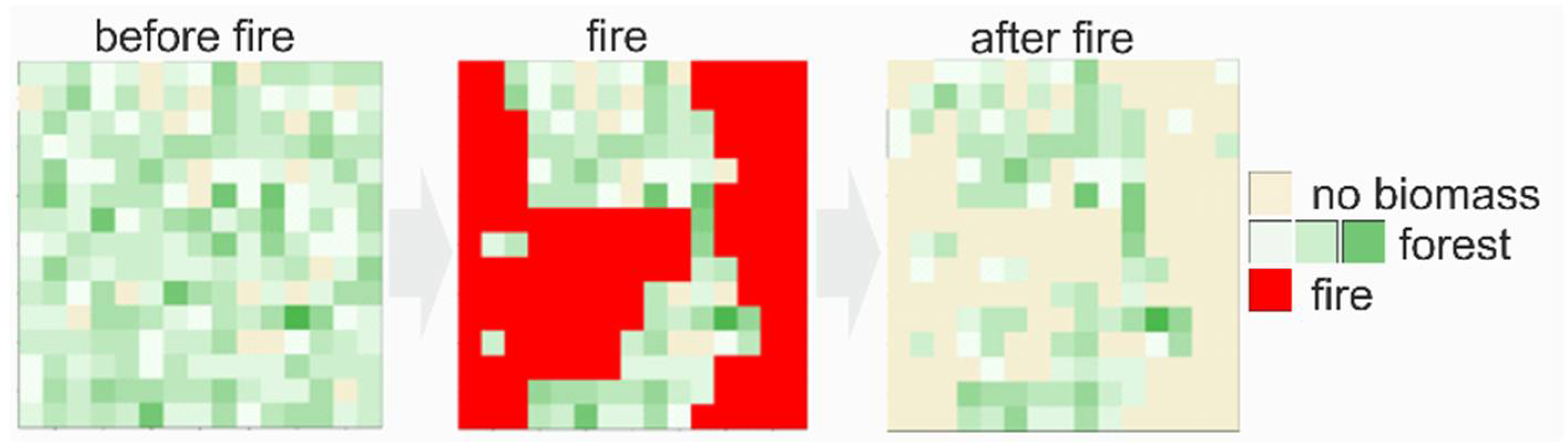
The heterogeneity of biomass in a virtual landscape before the simulated fire (left), during the fire (middle), and after the fire (right). Here, the green level indicates the amount of aboveground biomass; brown corresponds to an area without biomass in the forest. The spread of the simulated fire is shown in red. Until the fire event, the forest was simulated undisturbed on an area of 9 hectares (300 m × 300 m; one pixel has the size of 20 m × 20 m). After 250 years of simulation, a large-scale fire was realized (here: fire size 60%, intensity 0.67). Not all trees die in the fire area, and thus parts of the fire area still show biomass values after the fire event. Please note, in this schematic visualization only a virtual landscape is shown.
Figure 8.
The heterogeneity of biomass in a virtual landscape before the simulated fire (left), during the fire (middle), and after the fire (right). Here, the green level indicates the amount of aboveground biomass; brown corresponds to an area without biomass in the forest. The spread of the simulated fire is shown in red. Until the fire event, the forest was simulated undisturbed on an area of 9 hectares (300 m × 300 m; one pixel has the size of 20 m × 20 m). After 250 years of simulation, a large-scale fire was realized (here: fire size 60%, intensity 0.67). Not all trees die in the fire area, and thus parts of the fire area still show biomass values after the fire event. Please note, in this schematic visualization only a virtual landscape is shown.

Figure 9.
Simulated aboveground biomass (a) and carbon fluxes (b) after a fire event. A large-scale fire was simulated in the year 250. The development of aboveground biomass per shade-tolerance is shown on the left-hand side. In addition, the gross primary production (GPP), tree respiration, net primary production (NPP), and mortality for the simulated forest area are shown on the right-hand side. Mortality is without burnt trees.

Figure 10.
Simulated net ecosystem exchange after a fire event. Positive values correspond to net carbon sequestration in the forest. In the year 250, a large-scale fire was simulated, which led to a strong carbon source. (a) Annual carbon flux (NEE) and (b) cumulative carbon flux. The red area in (b) indicates the cumulative carbon flux before the forest fire.

Figure 11.
Simulated aboveground biomass for each plant functional type (PFT; climax green, pioneer red, mid-tolerance purple) without fire events (a) and after numerous fire events (b). On average, there is a fire in this region every 4 years. (c) Comparison of the species composition for an undisturbed and disturbed forest (here, the biomass fraction of each plant functional type serves as a proxy for diversity). odm = organic dry matter.

Figure 12.
Simulated carbon balance (net ecosystem exchange) over time in a tropical forest without fires (a) and with recurrent fires on average every 4 years (b). Positive values correspond to carbon sink behavior. (c) Cumulative carbon balance of both scenarios.
Figure 12.
Simulated carbon balance (net ecosystem exchange) over time in a tropical forest without fires (a) and with recurrent fires on average every 4 years (b). Positive values correspond to carbon sink behavior. (c) Cumulative carbon balance of both scenarios.

Figure 13.
Simulated species diversity for different fire frequencies. In each fire scenario, forest fires were simulated with a frequency of 1 to 10 fires per decade. The parameters are the same as in the standard fire scenario (see Table 1). The species diversity is described with the normalized Shannon Index (standard Shannon Index divided by ln(6)). For this index, the relative biomass fraction of each plant functional type is calculated over the last 300 years of simulation (in total, 6 plant functional types).


Table 1.
Parameter of the fire model ForFire and parameter values for the study region for the scenario where repeated fire events are simulated. For the scenario with only one fire event, the parameters are S = 60% and fsev = 0.67).
Table 1.
Parameter of the fire model ForFire and parameter values for the study region for the scenario where repeated fire events are simulated. For the scenario with only one fire event, the parameters are S = 60% and fsev = 0.67).
| Parameter | Description | Parameter Value for This Study |
|---|---|---|
| Fire frequency F | mean time between two fire events | 4 years |
| Fire size S | average size of a fire (here: 2 ha) in relation to the total size of the simulated forest (here: 9ha) | 20% |
| Fire severity fsev | indicator (0–1) for the strength and type of fire (light ground fire or strong crown fire) | 0.55 |
Table 2.
Species grouping with fire tolerance at Mt. Kilimanjaro region. Grouping of all tree species in the study area into six species groups according to maximum height and shade tolerance (for full species list, see Appendix A). This species grouping into plant functional types (PFT) was already investigated in former studies [32,33]. In this study, only a fire tolerance was assigned to each species group.
| PFT | Maximum Height [m] | Shade Tolerance | Exemplary Tree Species | Fire Tolerance |
|---|---|---|---|---|
| 1 | >33 | shade tolerant | Strombosia scheffleri | 2 |
| 2 | 16–33 | shade tolerant | Heinsenia diervilleoides | 1 |
| 3 | 16–33 | medium shade tolerant | Ficus sur | 1 |
| 4 | 16–33 | shade intolerant (pioneer) | Polyscias albersiana | 4 |
| 5 | <16 | shade tolerant | Leptonychia usambarensis | 2 |
| 6 | <16 | shade intolerant (pioneer) | Cyathea manniana | 2 |
Publisher’s Note: MDPI stays neutral with regard to jurisdictional claims in published maps and institutional affiliations. |
© 2021 by the author. Licensee MDPI, Basel, Switzerland. This article is an open access article distributed under the terms and conditions of the Creative Commons Attribution (CC BY) license (https://creativecommons.org/licenses/by/4.0/).
Share and Cite
MDPI and ACS Style
Fischer, R. The Long-Term Consequences of Forest Fires on the Carbon Fluxes of a Tropical Forest in Africa. Appl. Sci. 2021, 11, 4696. https://0-doi-org.brum.beds.ac.uk/10.3390/app11104696
AMA Style
Fischer R. The Long-Term Consequences of Forest Fires on the Carbon Fluxes of a Tropical Forest in Africa. Applied Sciences. 2021; 11(10):4696. https://0-doi-org.brum.beds.ac.uk/10.3390/app11104696
Chicago/Turabian StyleFischer, Rico. 2021. "The Long-Term Consequences of Forest Fires on the Carbon Fluxes of a Tropical Forest in Africa" Applied Sciences 11, no. 10: 4696. https://0-doi-org.brum.beds.ac.uk/10.3390/app11104696
Note that from the first issue of 2016, this journal uses article numbers instead of page numbers. See further details here.