
Performance Prediction and Design of Stratospheric Propeller


School of Aeronautics Science and Engineering, Beihang University (BUAA), Beijing 100191, China
*
Author to whom correspondence should be addressed.
Appl. Sci. 2021, 11(10), 4698; https://0-doi-org.brum.beds.ac.uk/10.3390/app11104698
Submission received: 22 April 2021
/
Revised: 14 May 2021
/
Accepted: 19 May 2021
/
Published: 20 May 2021
(This article belongs to the Section Aerospace Science and Engineering)
Abstract
:Featured Application
It provides a convenient propulsion force calculation method for the overall design of a stratosphere airship.
Abstract
In this paper, a performance prediction method is proposed for the design of a stratospheric propeller. The Spalart–Allmaras (S–A) model was used to calculate the airfoil performance of FX63, and the polynomial fitting method was utilized to establish the airfoil database of the lift and drag coefficient. A computational fluid dynamics (CFD) model was applied at different altitudes to prove the feasibility of the method. The CFD results were compared with the results of the vortex theory and prediction; the prediction result accuracy was improved compared with that of the vortex theory over a greater range of advance ratios. The airfoil performance data requirements and the number of iterative calculations were reduced. These results indicate that the proposed propeller design meets the requirements of stratospheric airship propulsion systems.
1. Introduction
The capability to fly continuously for months in the stratosphere is an elusive goal. Stratospheric airships have enormous potential for long-endurance vehicles, which do not need to stay in motion to remain in the air, since lift is generated through the buoyancy effect rather than aerodynamics. The efficient propulsion of propellers is essential for the maneuverability and sustainability of airships and cannot be achieved through turbojet and turbofan engines [1,2,3,4,5].
However, the environment in the stratosphere, which is above 20 km, has a much lower air density. Additionally, the velocity of advance of a stratospheric airship is lower than 30 m/s, which is extremely low. The low Reynolds number and small advance ratio create a significant challenge for the design of an efficient propeller.
The airfoil of high-altitude vehicles was researched by Prof. Michael S. Selig [6,7]; the aerodynamic characteristics of six typical low-Reynolds-number, high-lift, and low-resistance airfoils were analyzed, and wind tunnel experiments were carried out. Angleo [8] proposed a method of designing the chord length and twist angle to maximize propeller efficiency. Xiang [9] improved Angleo’s method to align it with the requirements of engineering applications.
Rankine [10] and Froude [11] first developed the theory of propellers in the 19th century, and Drzewiecki [12] proposed the blade element theory, which neglected the induced velocity of the propeller. The design method based on minimum induced losses was firstly proposed by Betz [13] and Goldstein [14]. Theodorsen’s [15] research indicated that the Betz condition for minimum energy loss could also be applied in heavy disk loadings. Glauert [16] discovered an approximation of the flow around helicoidal vortex sheets, which is better if the advance ratio of the propeller is smaller, and the result improves as the number of blades increases.
Numerical simulation technology has been widely used in propeller performance calculations with the development of computer technology. The k–ε turbulence model was used by Wang [17] to simulate the performance of a high-altitude propeller, and the result was in good agreement with the scaled wind tunnel experiment. Xiang [18] proposed an improved design method of propellers, which could be optimized under specific operative condition and according to the profile distribution along the blade, and the wind tunnel test showed that the method was feasible.
Reasonable accurate performance prediction could be obtained based on vortex theory and blade element theory [19,20]. Liu [21] studied the propeller’s aerodynamic characteristics utilizing the vortex theory and a propeller model [22,23], and the results indicated that the S–A model is more suitable for calculating aerodynamic parameters. The performance predicted by the vortex theory was similar to that determined by scale wind tunnel tests. However, in the design process, the airfoil data of each section are needed for calculating the performance of the propeller.
The S–A model was performed in Fluent to calculate the airfoil performance at different angles of attack and Reynolds numbers. The performance curves of the lift and drag coefficient underwent polynomial interpolation to obtain the database, which was used to calculate the performance of the propeller. The CFD model with different mesh numbers was applied to verify the mesh independence, and the CFD method at different altitudes was applied with the similarity theory to prove the feasibility of the method.
In this paper, a prediction method is proposed to reduce calculations or experimental times and to predict a propeller’s performance on the basis of characteristic blade element performance. The prediction parameters are discussed, and a realistic and accurate prediction model is obtained which reduces the calculation amount with respect to the vortex theory, in regard not only to airfoil performance calculation, but also to propeller performance calculation.
2. Methodology
The blade element theory is typically used to predict the performance of a propeller. The blade is divided into a finite number of tiny segments called blade elements, and the aerodynamic performance of each blade element can be obtained according to the airfoil theory. The blade element is integrated along the radial direction to obtain the total aerodynamic performance of the blade.
Figure 1 presents the forces and velocities acting on the blade element, where is the free stream speed, is the axial induction velocity, is the tangential induction velocity, and V is the total velocity of the actual airflow; is the angular velocity of the propeller, and r is the radial position of the blade element; is the induced angle of attack, is the angle of actual airflow, is the pitch angle, and is the interference angle, which is given by:
The axial and tangential induction factors are defined as follows:
The angle of actual airflow is as follows:
The angle of attack , the velocity of the actual airflow V, and the local Reynolds number Re are given by:
The thrust and torque forces acting on the blade element are as follows:
where b is the chord length of the blade element. CTV and CFV are obtained from the geometric relationship shown in Figure 1; CL and CL can be determined by Re and α.
Equation (5) is integrated into Equation (7), and the lift and torque acting on the propeller are given by:
The momentum theory equations are shown below:
Combining Equations (9) and (10), we obtained:
where is the solidity ratio of the propeller, and F is the Prandlt momentum loss factor.
where f is given by:
where is the flow angle of the blade tip, and is the dimensionless radius. At the beginning of the calculation, the value of is unknown, and the error is not too large to replace .
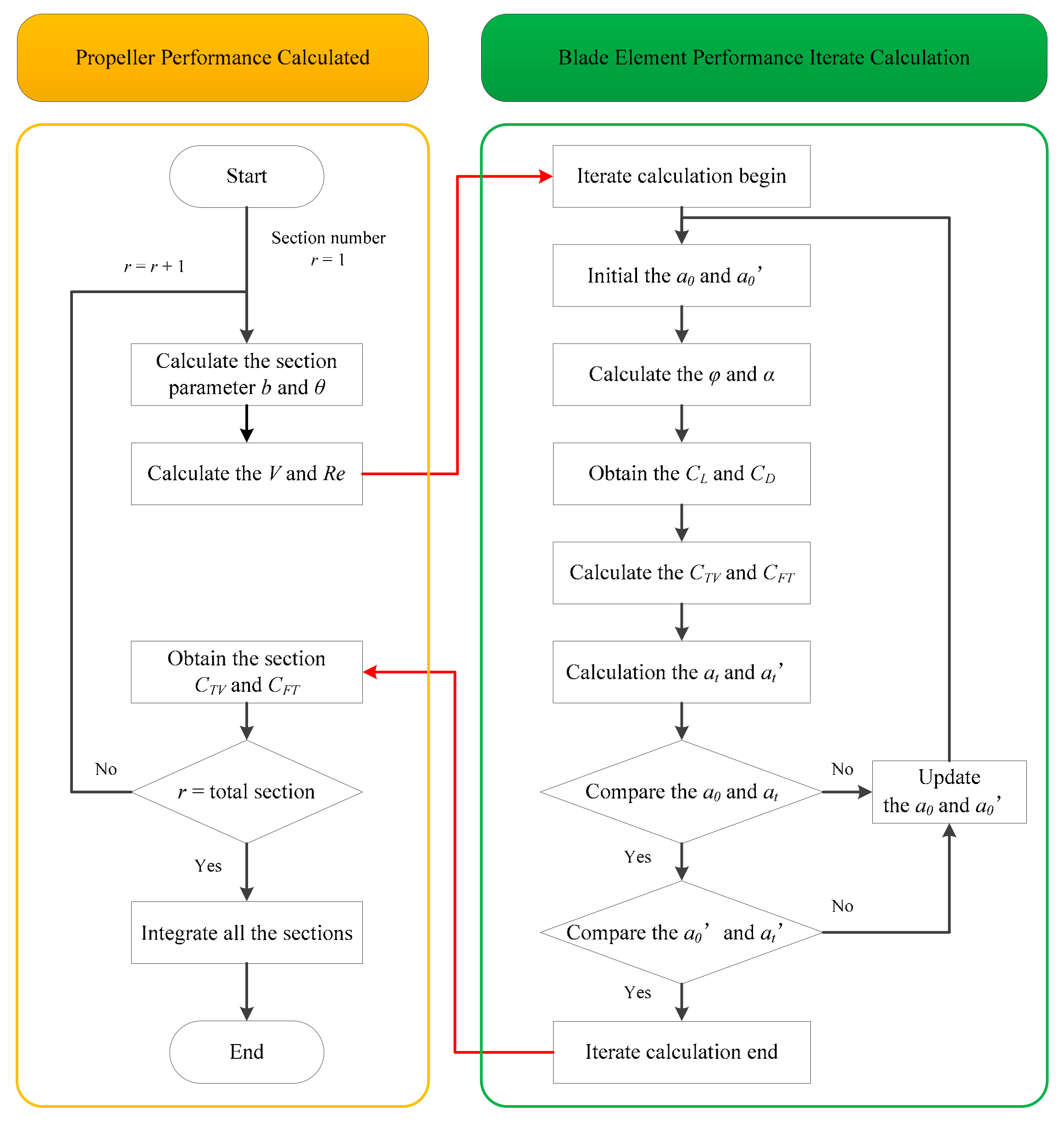
An iterative method is used to calculate the axial and tangential induction factors and : (1) set the initial value of and ; (2) calculate the angle of actual flow ; (3) according to the pitch angle , calculate the angle of attack ; (4) obtain the and that form the lift and drag curves of the airfoil respectively; (5) use Equation (8) to calculate the and ; (6) the and are calculated by Equation (11); (7) comparing and , and , if they are beyond the allowable error range, repeat steps (2) to (7); otherwise, the final and are generated, and the iteration is ended. The iterative process is shown in Figure 2.
The thrust and torque of the propeller are obtained by:
The dimensionless parameter thrust coefficient CT, the power coefficient CP, and the efficiency η are defined as follows:
where λ is the advance ratio, given by:
3. Propeller Design
According to the propulsion system requirements of the stratospheric airship design, the design indexes of the propeller were determined and are listed in Table 1. The required advance velocity appeared to be 20 m/s; the required thrust resulted to be larger than 100 N, and the efficiency larger than 70%.
A two–blade propeller was selected due to its low speed and large diameter, and the FX63 airfoil was selected for the propeller. The Mach number of the propeller tips was restricted as follows:
where c is the local sound velocity.
The propeller geometry is defined by the pitch angle θ and the chord length b along the radius of the blade from the hub to the tip, which is determined as follows:
where θchar is the characteristic pitch angle of the propeller, D is the diameter of the propeller, and = 0.1, 0.2, …, 1.
4. Performance Prediction
The aerodynamic loss of the propeller is mainly concentrated on the root and tip. As the root must be strong enough to withstand loads such as the rotating centrifugal force and the bending moment of the whole propeller, it is usually too thick to exhibit good aerodynamic performance. The vortex at the tip increases the induced aerodynamic resistance and reduces the thrust, and if the rotating speed is too high, the tip is prone to generating shock loss. Therefore, the thrust is mainly generated from 0.7R to 0.9R of the blade. The performance of the propeller is determined among these sections, and the propeller performance can be predicted through the characteristic blade element rchar. The thrust and torque of the propeller can be given by:
where r0 is the prediction parameter that indicated the coverage on both sides of the characteristic blade element. In this article, 0.75R is selected as the characteristic blade element. Equation (22) and the efficiency of the propeller can be given as:
The thrust T and the torque M are predicted by the 0.75R element and ; the 0.75R element performance is obtained by iterate calculation ( will be discussed later). The efficiency is independent of and depends on the 0.75R element performance. This prediction method only needs an iterative calculation of the performance of , rather than of the whole section of the propeller; a lower amount of calculation is also required to determine the airfoil performance.
5. Finite Element Analysis
5.1. Airfoil Model
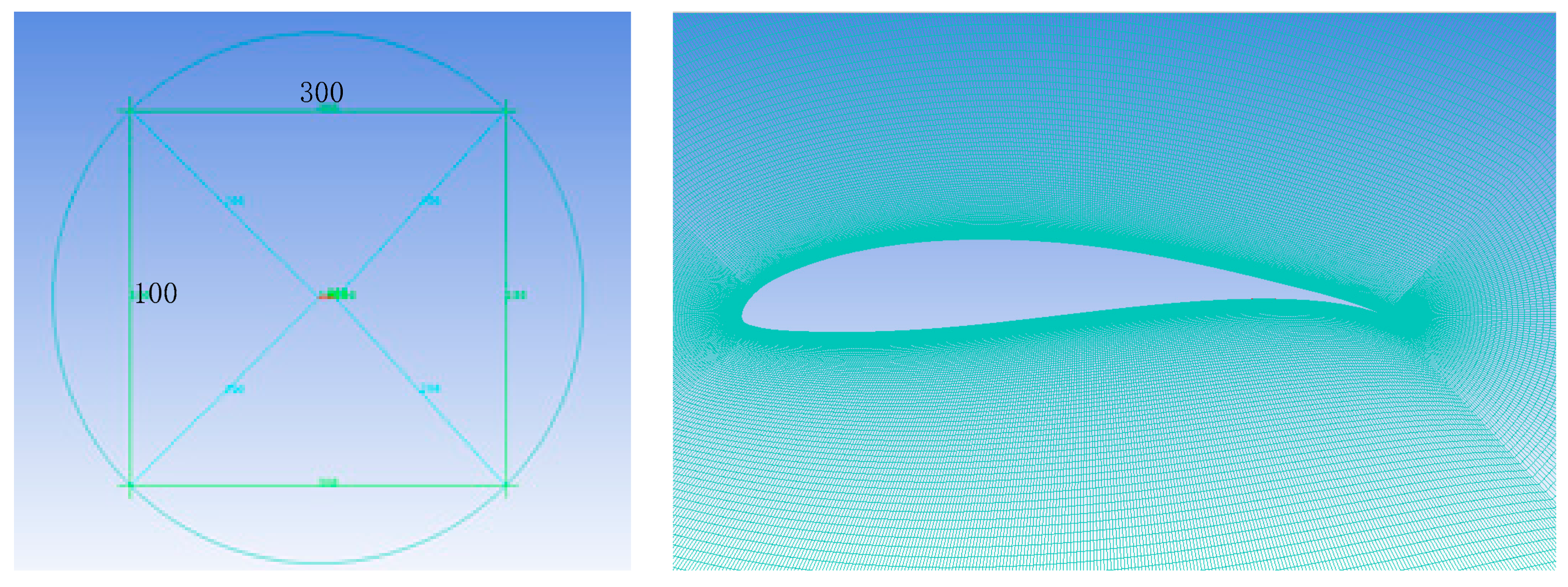
ANSYS ICEM was used to generate a two-dimensional O-Block mesh of the fluid domain, in which the number of grid points was 300 × 100. A density-based solver was applied in ANSYS Fluent, and the Reynolds average Navier–Stokes (RANS) equation and the S–A turbulence model were adopted. The Green–Gauss node-based scheme was selected as the discretization scheme, and the second-order upwind scheme was selected for turbulence equation discretization. The computational domain was 15 times the chord length. The far-field pressure was used as the boundary condition, and the airfoil was set as the wall boundary. The residual value was required to be below 1 × 10⁻⁶ to ensure convergence. The mesh of the airfoil is shown in Figure 3.
5.2. Propeller Model
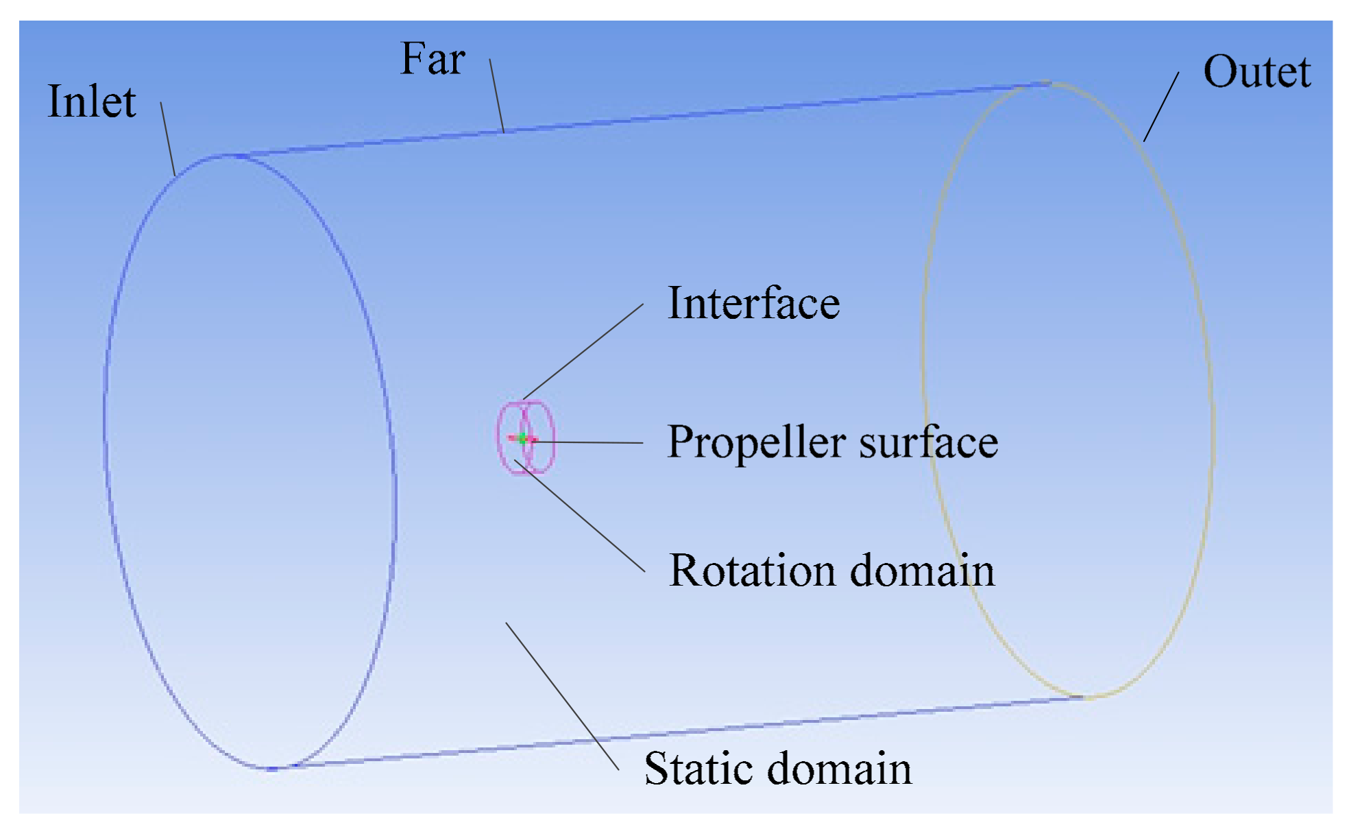
A three-dimensional mesh was generated in ICEM. Figure 4 shows the computational domain, which consisted of two components, an internal rotation domain, and an external static domain. The upstream distance of the static domain was 10 times the diameter of the propeller, the downstream one was 20 times, and the diameter of the static domain was 10 times the diameter of the propeller. The rotation domain’s speed is , whereas the static domain is stationary. The interface boundary condition was used as the exchange data between the static and the rotation domains, the velocity inlet and pressure outlet were adopted as the boundary conditions of the static domain, and the surface of the propeller was set as the wall.
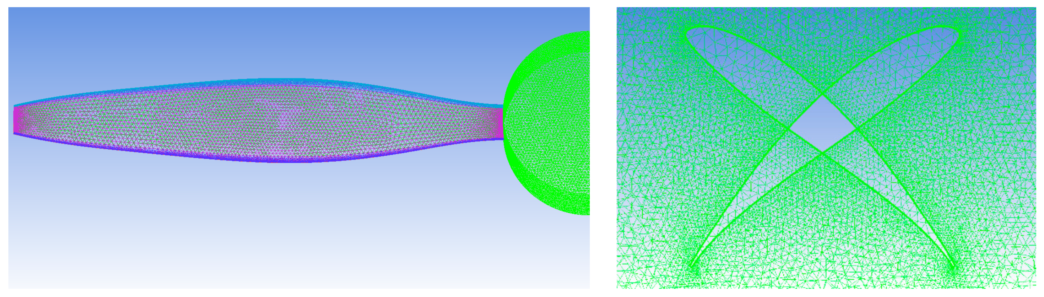
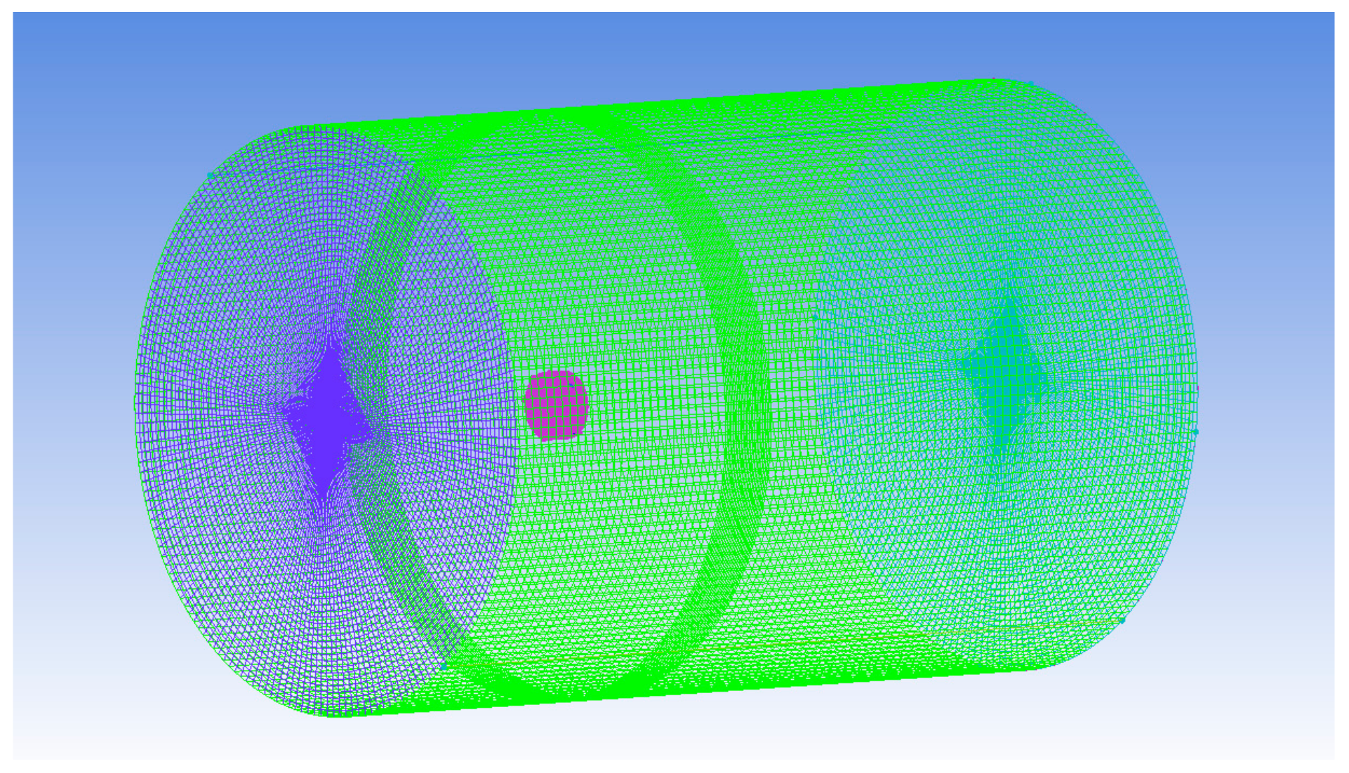
The rotational domain was composed of 5.55 million meshes, the blade surface was a triangular mesh, and the boundary layer around the surface was an hexagonal mesh, which is shown in Figure 5. A tetrahedral mesh was used to fill the space between the propeller surface and the interface.
The static domain is shown in Figure 6, which composed of 1.97 million hexagonal meshes, which were generated based on a three-dimensional O-Block.
FLUENT with a pressure-based solver was used to perform the CFD analyses. The control equation was discretized using the finite volume method, and the RANS equation and the k–ω SST Low–Re corrections turbulence model were adopted. The multiple reference frame (MRF) model was used to calculate the rotational motion of the propeller. The pressure–velocity coupling algorithm and the second-order upwind scheme were applied. The parameter y+ is the dimensionless wall distance for a wall-bounded flow, which was required to be less than 1 according to the boundary layer mesh on the propeller. The CFD results showed that y+ was approximately 0.7 along the blade length in this model.
According to the propeller similarity theory, the performance at different altitudes should be consistent when the Reynolds number and the advance ratio are equal.
For the same propeller model, D0 = D1 the scaling ratio can be determined by:
6. Result and Discussion
6.1. Airfoil Performance of FX–63
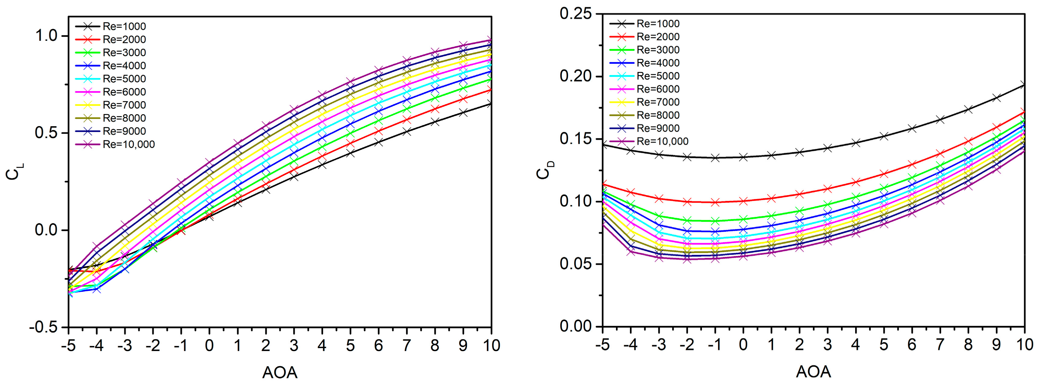
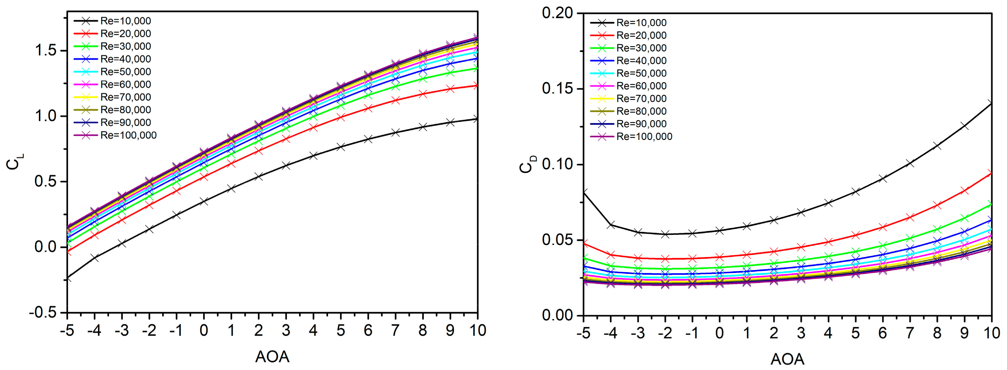
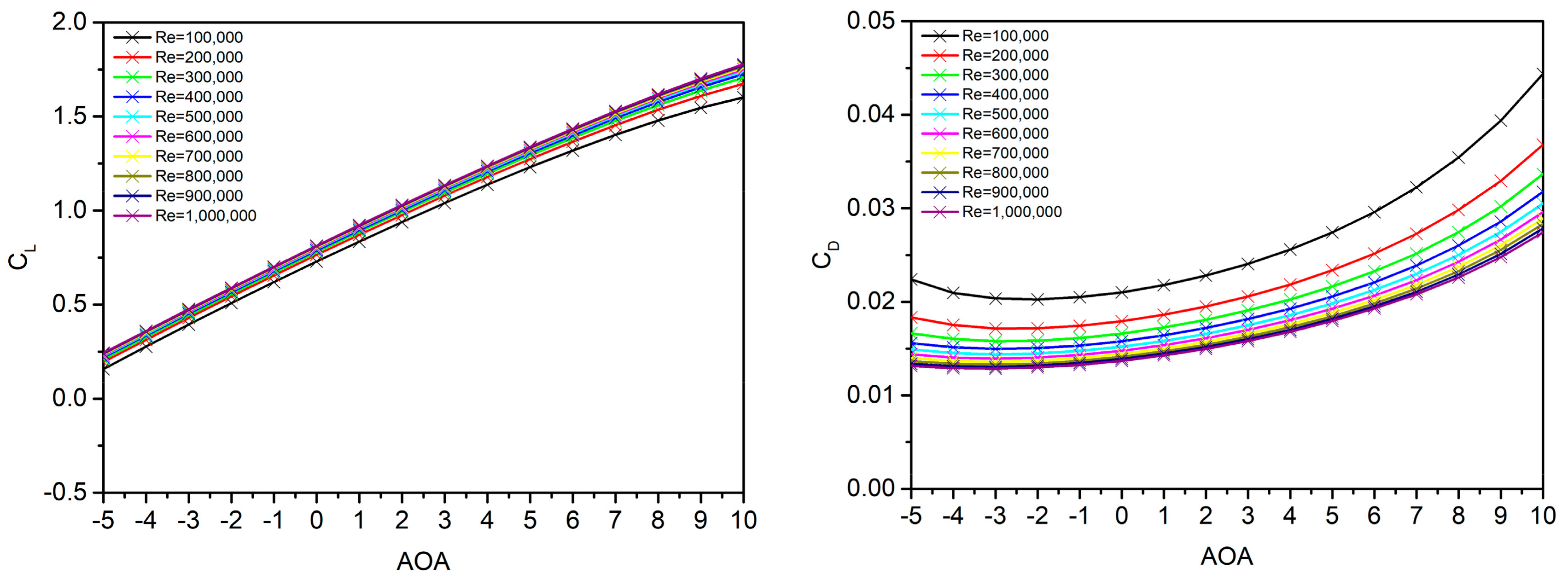
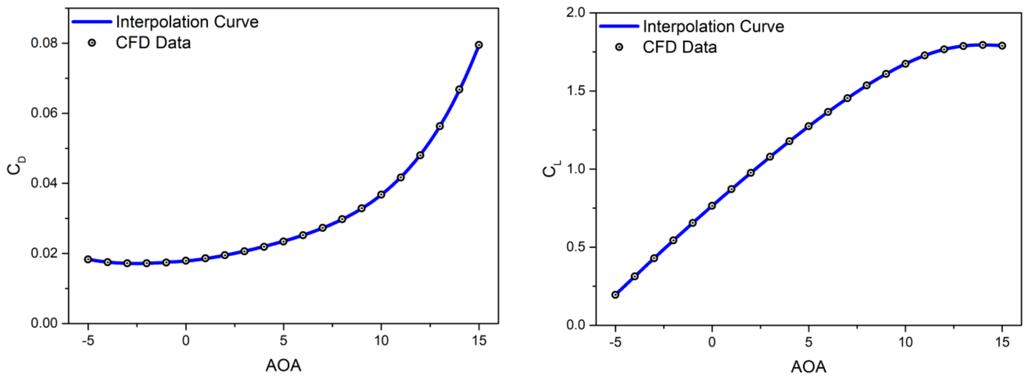
The blade element performance was required to design and predict the performance of the propeller. A CFD simulation was applied to obtain the lift and drag coefficient curves of the FX63 airfoil for different Reynolds numbers and angles of attack (AOA). The range of Reynolds numbers changed from 1000 to 100,000, and the AOA changed from −5° to 15°. The lift and drag coefficient curves are presented in Figure 7, Figure 8 and Figure 9.
The polynomial fitting method in MATLAB was used to interpolate the lift and drag coefficient curves, when the Reynolds number increased from 1000 to 1,000,000. The airfoil lift and drag coefficient curves at Re = 8000 and 200,000 are presented in Figure 10 and Figure 11, respectively. The polynomial curves were in good agreement with the CFD data. The polynomial equations are reported below the figures.
6.2. Performance of the Designed Propeller
According to the performance calculation process, chord length b and pitch angle are the initial input condition. In the different sections, b is fixed once the diameter of the propeller is determined. To meet the rated thrust, is adjusted, and the iterative calculation needs to be performed with the data of airfoil performance.
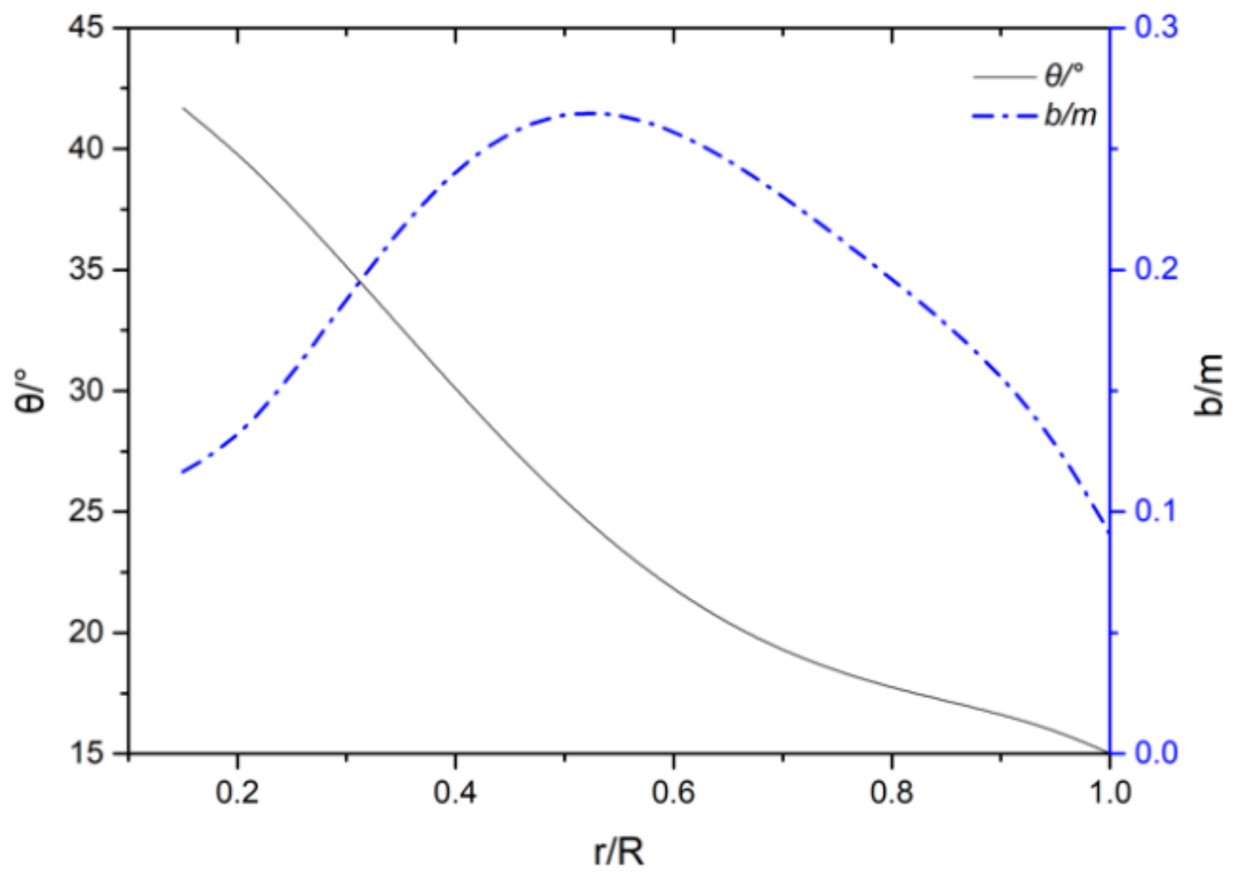
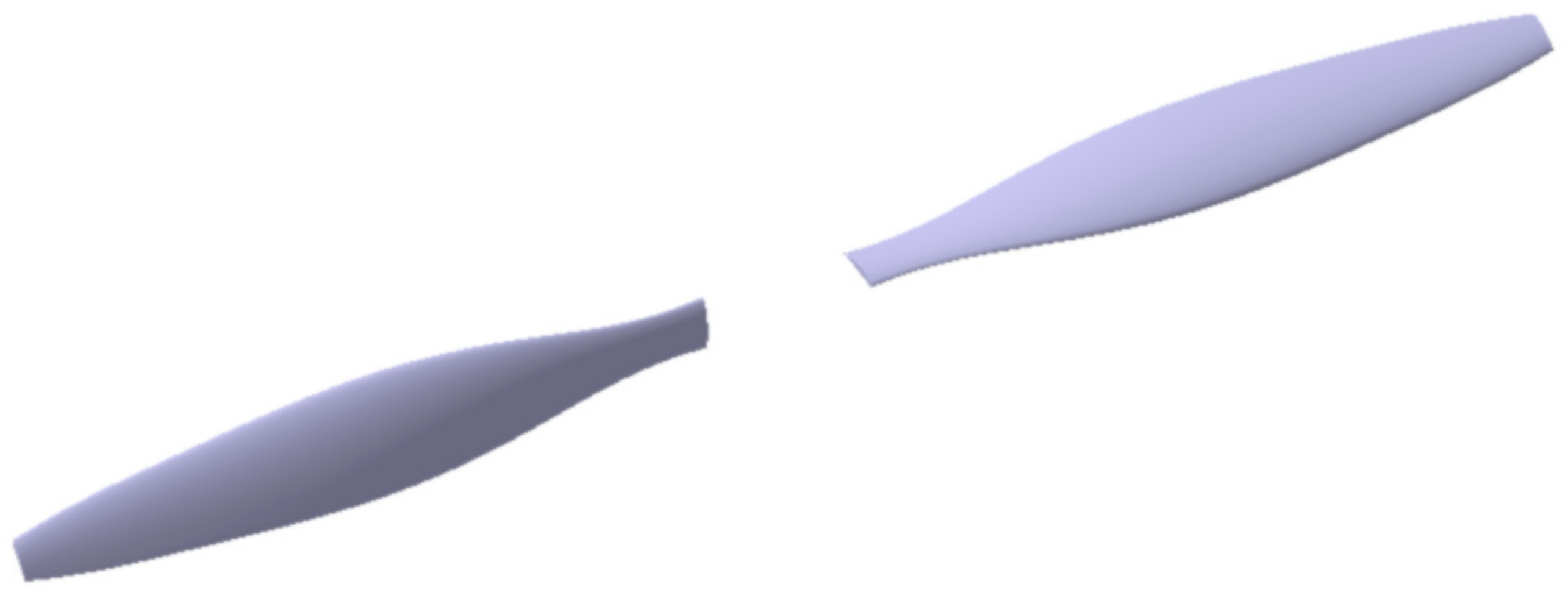
The shape parameters are shown in Figure 12. The pitch angle decreased with the increase of . The chord length first increased, reached a maximum value near 0.5R, and then decreased. The 3D solid model of the propeller is shown in Figure 13 and was constructed according to the design parameters.
Figure 14 shows the angle of attack and interference angle of the propeller, which were designed according to the vortex theory and standard strip analysis. The interference angle affects the angle of attack and, consequently, the aerodynamic performance of the blade. The AOA was negative near the root, and most of the blade section showed a small AOA.
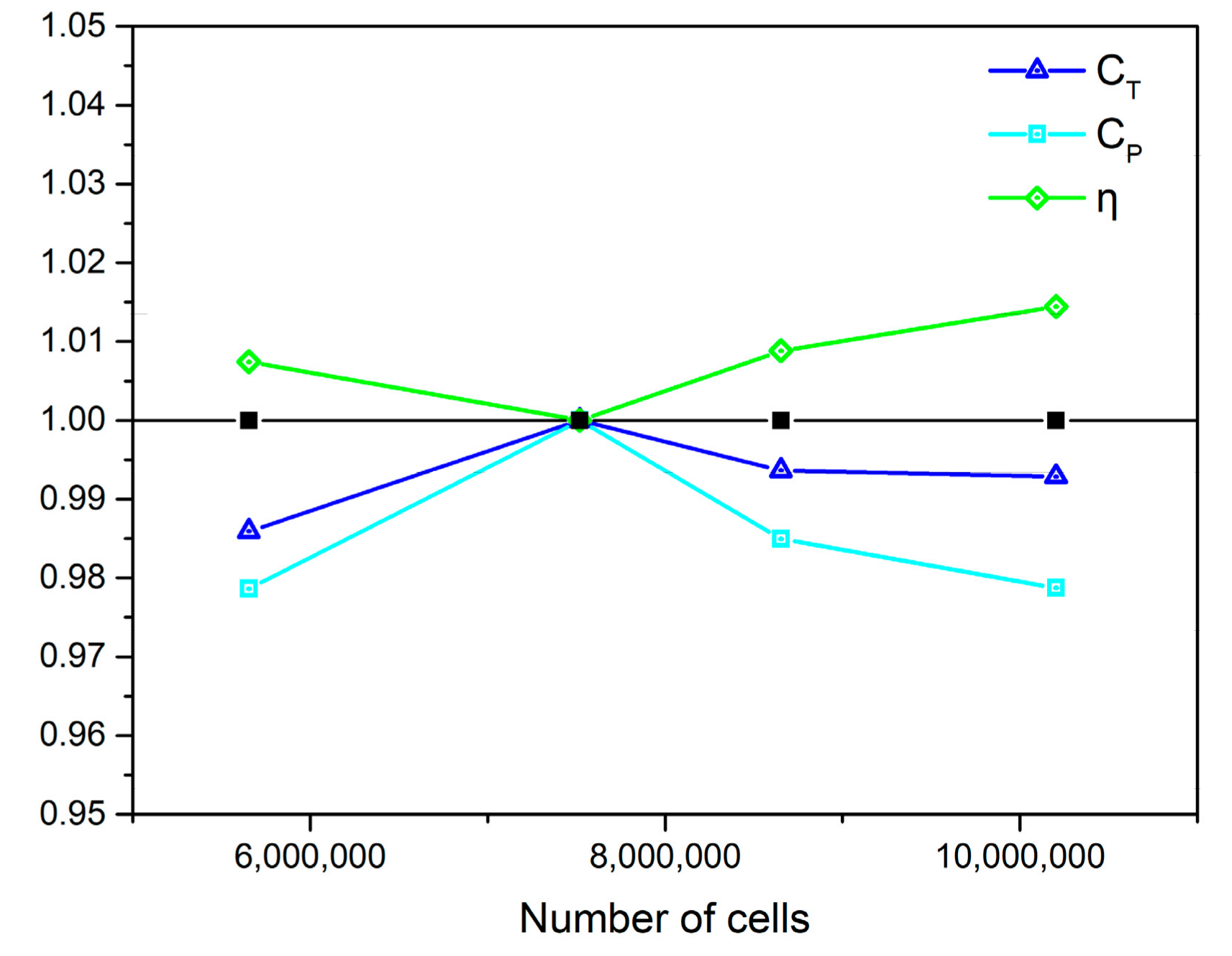
The deviation of four different mesh qualities is shown in Figure 15. The cell number of the coarse mesh was 5.65 million, the mesh used consisted of 7.52 million cells, the refined mesh comprised 10.2 million cells, and the other mesh 8.65 million cells. The maximum deviation from the mesh used was less than 1.41% for the thrust coefficient, 2.14% for the power coefficient, and 1.44% for the efficiency. The results of mesh independency verification showed that the number of cells had a little influence on the results; a mesh with 7.52 million cells was reliable and was chosen for CFD simulation in this paper.
The CFD simulation at H = 15 km, 18 km, and 20 km was performed using the mesh model mentioned above, and the results are shown in Figure 16. The variation tendencies of , , and were approximately the same. The and of H = 15 km and H = 18 km deviated slightly towards those of H = 20 km when 0.7, and the deviation decreased with the increase of . The values at the three altitudes were almost identical within the change range of . The altitude had almost no effect on the aerodynamic performance of the designed propeller, and the simulation method was reliable and correct.
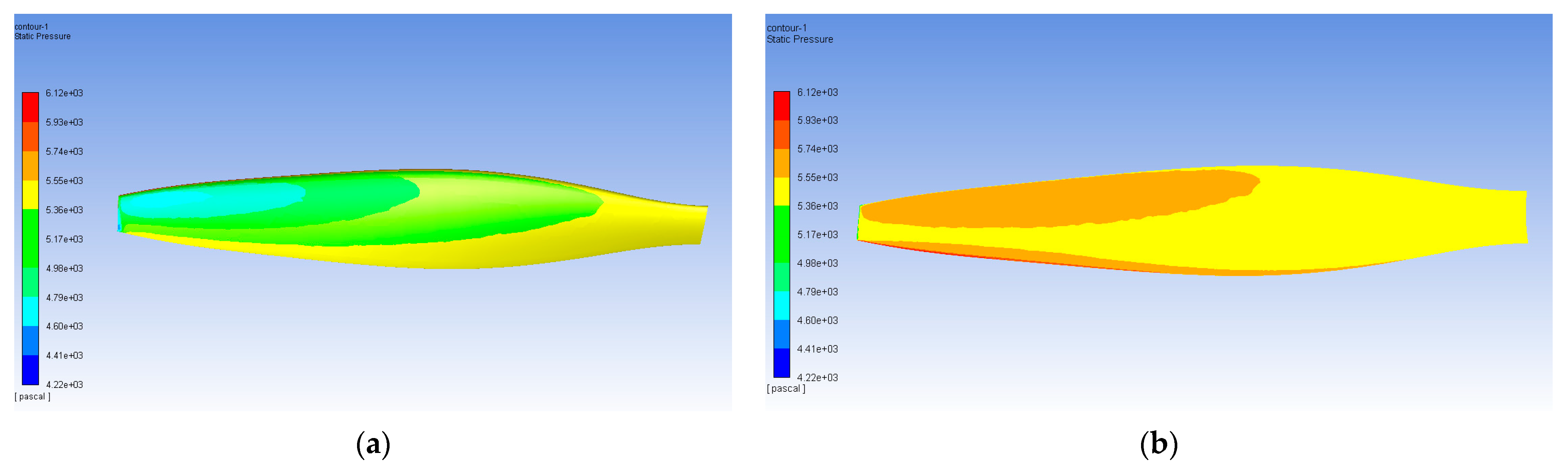
Figure 17 shows the pressure contour of the designed propeller at the design point. The pressure on the upper surface decreased from the root to the tip and from the leading edge to the trailing edge, and the minimum pressure occurred from 0.75R to 0.98R. The pressure on the lower surface increased from root to tip and from the middle to the trailing and leading edges, and the maximum pressure occurred from 0.61R to 0.99R.
6.3. Performance Prediction for the Designed Propeller
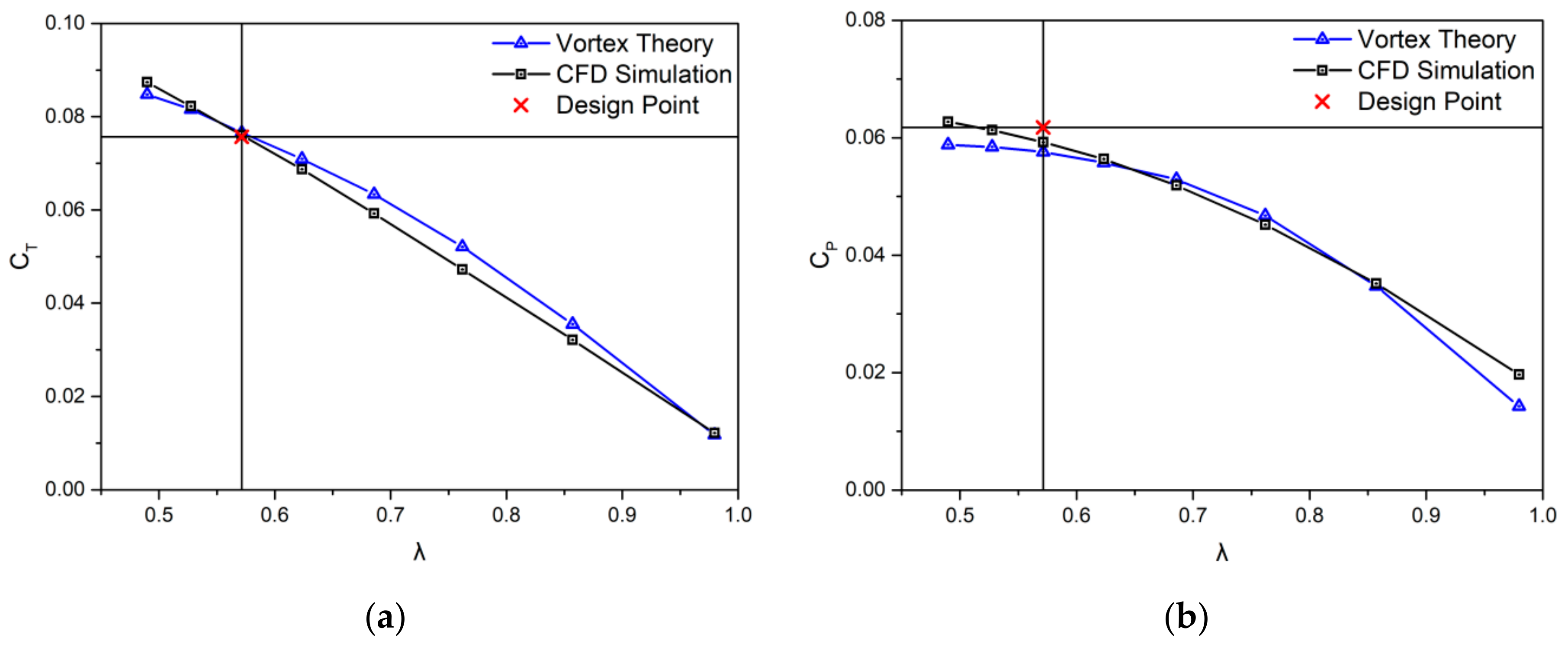
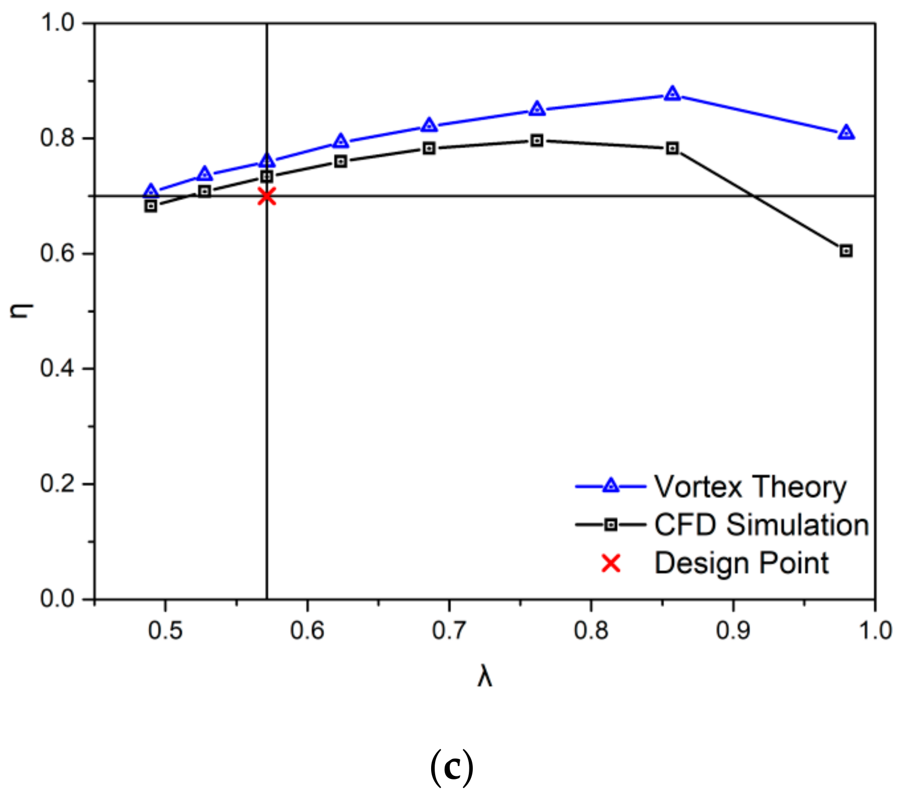
The designed propeller performances calculated using the vortex theory and simulated in CFD are compared in Figure 18. The performance predicted by the vortex theory appeared in good agreement with that determined by CFD simulation. This result indicates that the prediction value of was lower than the simulation value when 0.55 and started to deviate from the simulation value when 0.75, when the deviation began to decrease. The prediction value of was higher than the simulation value when 0.65 0.85. The variation tendency of between the prediction and the simulation values was the same, and the prediction value was higher than the simulation value in the entire range of .
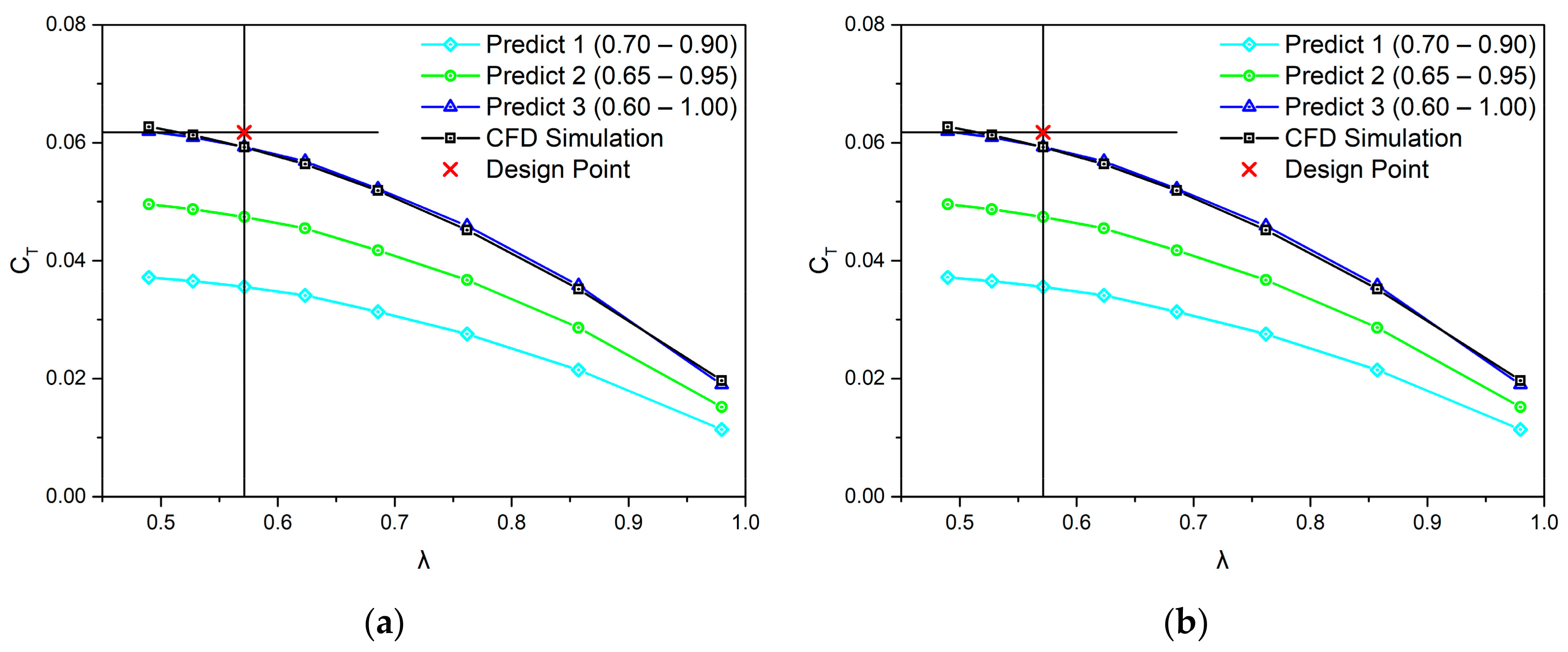
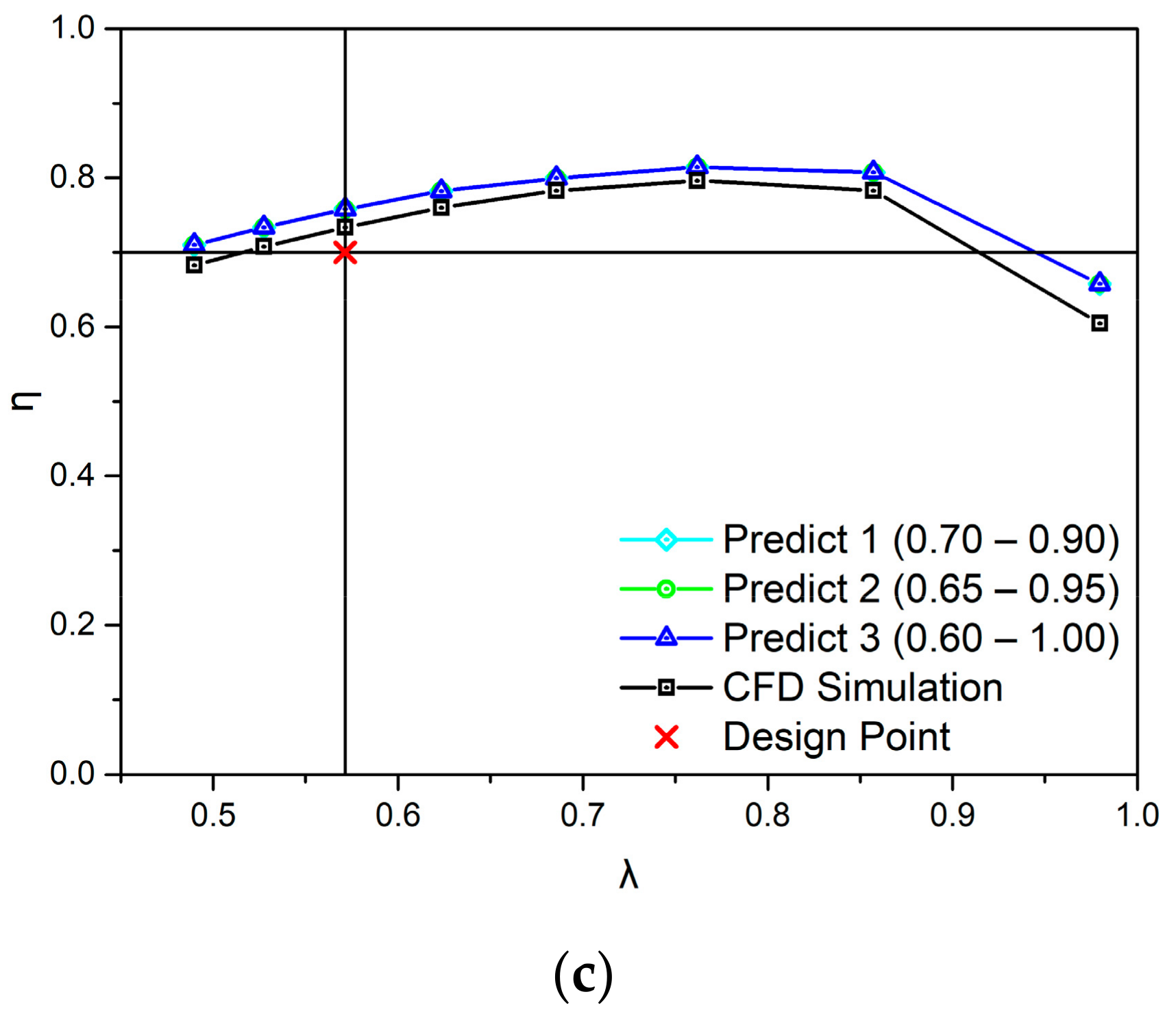
Although the vortex theory can determine the performance of the propeller, it must iteratively make computations for each section of the blade. Using the prediction method mentioned above, the aerodynamic performance of the propeller could be predicted based on the blade element performance at 0.75R, thus reducing the number of iterative calculations. The values 0.15R, 0.2R, and 0.25R were calculated by Equation (22) to predict the propeller performance, which meant the propeller performance was attributed to 0.6R–0.9R, 0.55R–0.95R, and 0.5R–R. These results were expressed as Predict 1, Predict 2, and Predict 3, respectively.
The propeller performances predicted based on the blade element at 0.75R and simulated in CFD are compared in Figure 19. All three predictors had the same variation tendency as the simulation in , , and , but the Predict 1 and Predict 2 values of and were far lower than the simulation value. The value of Predict 3 was higher than the simulation value, and the deviation decreased with increasing . The value of Predict 3 almost coincided with the simulation value, causing the value of Predict 3 to be higher than the simulation value. The values of the three predictions were the same according to Equation (24).
Table 4 indicates that the prediction accuracy of Predict 3 was the same for the three aerodynamic parameters as that of the vortex theory at the design point. For 0.25R, Predict 3 was in accordance with the result in Figure 17. Predict 3 was more similar to the CFD simulation value within a larger range, and the tendency was more consistent; a higher predicted value and a lower predicted value were conducive to designing the propeller.
7. Conclusions
In this paper, the airfoil performance of FX63 was obtained by CFD simulation, and the polynomial fitting method was utilized to establish the airfoil database of the lift and drag coefficients. The results indicated that the propeller design met the requirements of stratospheric airship propulsion system. The CFD model of the propeller was proven to be reliable at different altitudes with the same Reynolds number and advance ratio, and the performance curves were almost identical.
This paper proposes a method to predict the performance of a propeller for stratospheric airship based on the characteristic blade element, while reducing the amount of iterative calculations. The CFD results were compared with the results of the vortex theory and prediction; the prediction results accuracy was improved compared with that of the vortex theory over a greater range of advance ratios. The predicted deviation was 3.46%, of which was 0.12%, and was 3.33% when the character section was 0.75R and the predict parameter was 0.25R.
This study provides a convenient propulsion force calculation method for the overall design of the stratosphere airship. The propeller performance can be predicted only by the airfoil performance of the characteristic blade element, instead of requiring calculations through an airfoil performance database. This significantly reduces the number of CFD calculations or wind tunnel tests.
Author Contributions
Conceptualization, C.X. and G.T.; Funding acquisition, G.T.; Investigation, C.X.; Methodology, G.T. and Z.W.; Project administration, Z.W.; Resources, Z.W.; Software, C.X.; Validation, G.T.; Visualization, C.X.; Writing—original draft, C.X.; Writing—review & editing, C.X. All authors have read and agreed to the published version of the manuscript.
Funding
This research received no external funding.
Institutional Review Board Statement
Not applicable.
Informed Consent Statement
Not applicable.
Data Availability Statement
The data presented in this study are available on request from the corresponding author.
Conflicts of Interest
The authors declare no conflict of interest.
References
- Colozza, A.; James, D. Initial Feasibility Assessment of a High Altitude Long Endurance Airship; Technical Report CR–2003–212724; Analex Corp.: Los Angeles, OH, USA, 2003. [Google Scholar]
- D’Oliveira, F.; Melo, F.; Devezas, T. High-Altitude Platforms—Present Situation and Technology Trends. J. Aerosp. Tech. Manag. 2016, 8, 249–262. [Google Scholar] [CrossRef]
- Zhao, D.; Liu, D. Research status, technical difficulties and development trend of stratospheric airship. Acta Aeronaut. Astronaut. Sin. 2016, 37, 45–56. [Google Scholar]
- Wu, J.; Fang, X.D.; Wang, Z. Thermal modeling of stratospheric airships. Prog. Aerosp. Sci. 2015, 75, 26–37. [Google Scholar] [CrossRef]
- Xu, Y.; Zhu, W.; Li, J. Improvement of endurance performance for high-altitude solar-powered airships: A review. Acta Astronaut. 2019, 167, 245–259. [Google Scholar] [CrossRef]
- Selig, M.S.; Guglielmo, J.J. High-Lift Low Reynolds Number Airfoil Design. J. Aircr. 1997, 34, 72–79. [Google Scholar] [CrossRef] [Green Version]
- Selig, M.S.; Mcgranahan, B.D. Wind Tunnel Aerodynamic Tests of Six Airfoils for Use on Small Wind Turbine. J. Sol. Energy 2004, 126, 986. [Google Scholar] [CrossRef]
- D’Angelo, S.; Berardi, F.; Minisci, E. Aerodynamic Performance of Propellers with Parametric Considerations on the Optimal Design. Aeronaut. J. 2002, 106, 313–320. [Google Scholar]
- Xiang, S.; Wang, J.; Zhang, L. A design method for high efficiency propeller. J. Aerosp. Power 2015, 30, 136–141. [Google Scholar]
- Rankine, W.M.J. On the Mechanical Principles of the Action of the Propellers. Trans. Inst. Nav. Arch. 1865, 6, 13–30. [Google Scholar]
- Froude, W. On the Elementary Relation between Pitch, Slip and Propulsive Efficiency; Technical Memorandum, NASA–TM–X–61726; NTRS: Washington, DC, USA, 1878; Volume 19, pp. 22–33. [Google Scholar]
- Drzewiecki, S. Méthode pour la Détermination des Elements Mécaniques des Propulseurs Hélicoïdaux; Bulletin de l’Association Technique Maritime: Paris, France, 1892. [Google Scholar]
- Betz, A. Schraubenpropeller mit geringstem Energieverlust. Mit einem Zusatz von l. Prandtl. Gött. Nachr. 1919, 3, 193–217. [Google Scholar]
- Goldstein, S. On the vortex theory of screw propellers. Proc. R. Soc. A Math. Phys. Eng. Sci. 1929, 123, 440–465. [Google Scholar]
- Theodorsen, T. Theory of Propellers; McGraw–Hill Book Company: New York, NY, USA, 1948. [Google Scholar]
- Glauert, H. Airplane Propellers, Aerodynamic Theory; Division L; Durand, W.F., Ed.; Springer: New York, NY, USA, 1963; Volume IV, pp. 169–360. [Google Scholar]
- Wang, Y.; Liu, Z.; Tao, G. Numerical simulation of a high altitude propeller’s aerodynamic characteristics and wind tunnel test. J. Beihang Aeronaut. Astronaut. 2013, 39, 1102–1105. [Google Scholar]
- Xiang, S.; Liu, Y.-q.; Tong, G. An improved propeller design method for the electric aircraft. Aerosp. Sci. Tech. 2018, 78, 488–493. [Google Scholar] [CrossRef]
- Nigam, N.; Tyagi, A.; Chen, P. Multi-fidelity multi-disciplinary propeller/rotor analysis and design. In Proceedings of the 53rd AIAA Aerospace Sciences Meeting, Kissimmee, FL, USA, 5 January 2015. [Google Scholar]
- Morgado, J. Validation of New Formulations for Propeller Analysis. J. Propul. Power 2015, 31, 467–477. [Google Scholar] [CrossRef]
- Liu, X.; He, W. Performance Calculation and Design of Stratospheric Propeller. IEEE Access 2017, 5, 14358–14368. [Google Scholar] [CrossRef]
- Liu, P.; Ma, R.; Duan, Z. Ground Wind Tunnel Test Study of the Propeller of Stratospheric Airships. J. Aerosp. Power 2011, 26, 1775–1781. [Google Scholar]
- Liu, P.; Duan, Z.; Ma, L. Aerodynamics properties and design method of high efficiency-light propeller of stratospheric airships. In Proceedings of the 2011 International Conference on Remote Sensing, Environment and Transportation Engineering, Nanjing, China, 24–26 June 2011. [Google Scholar]
Figure 1.
Forces and velocities acting on the blade element.

Figure 2.
Iterative process for propeller performance calculation.

Figure 3.
Mesh of the airfoil.

Figure 4.
Domain and boundary of the propeller.

Figure 5.
Mesh near the propeller.

Figure 6.
Mesh of the propeller.

Figure 7.
FX63 airfoil performance for Re = 1000–10,000.

Figure 8.
FX63 airfoil performance for Re = 10,000–100,000.

Figure 9.
FX63 airfoil performance for Re = 100,000–1,000,000.

Figure 10.
FX63 airfoil performance at Re = 8000.

Figure 11.
FX63 airfoil performance at Re = 200,000.

Figure 12.
Shape parameters of the propeller.

Figure 13.
Solid model of the propeller.

Figure 14.
Angle of attack and interference angle of the propeller.

Figure 15.
Mesh independency verification.

Figure 16.
Propeller performance at different altitudes: (a) thrust coefficient; (b) power coefficient; (c) efficacy.
Figure 16.
Propeller performance at different altitudes: (a) thrust coefficient; (b) power coefficient; (c) efficacy.

Figure 17.
Pressure contour of the propeller at the design point: (a) upper surface of the blade; (b) lower surface of the blade.
Figure 17.
Pressure contour of the propeller at the design point: (a) upper surface of the blade; (b) lower surface of the blade.

Figure 18.
Comparison of the results from vortex theory with those form CFD simulation: (a) thrust coefficient; (b) power coefficient; (c) efficacy.
Figure 18.
Comparison of the results from vortex theory with those form CFD simulation: (a) thrust coefficient; (b) power coefficient; (c) efficacy.


Figure 19.
Comparison of predicted performance with results of CFD simulation: (a) thrust coefficient; (b) power coefficient; (c) efficacy.
Figure 19.
Comparison of predicted performance with results of CFD simulation: (a) thrust coefficient; (b) power coefficient; (c) efficacy.


Table 1.
The design index of propeller.
| Altitude | Velocity | Rated Speed | Rated Thrust | Diameter | Efficiency |
|---|---|---|---|---|---|
| 20 km | 10 m/s | 600 RPM | ≥100 N | ≤3.5 m | ≥70% |
Table 2.
Atmosphere conditions at different altitudes.
| H/km | T/K | P/Pa | ||
|---|---|---|---|---|
| 15 | 0.19367 | 216.65 | 12,044.5 | 1.4216 × 10⁻⁵ |
| 18 | 0.12164 | 216.65 | 7565.2 | 1.4216 × 10⁻⁵ |
| 20 | 0.08803 | 216.65 | 5474.9 | 1.4216 × 10⁻⁵ |
Table 3.
Scaling ratio at different altitudes.
| Altitude | Length | Density | Rotation Speed | Advance Speed |
|---|---|---|---|---|
| 15 | 1 | 2.200 | 0.454 | 2.200 |
| 18 | 1 | 1.382 | 0.724 | 1.382 |
| 20 | 1 | 1 | 1 | 1 |
Table 4.
Comparison of predicted value and simulate value at design point.
| = 0.57 | CFD Simulation | Vortex Theory | Predict 3 | ||
|---|---|---|---|---|---|
| Value | Value | Deviation | Value | Deviation | |
| 0.0760 | 0.0766 | 0.71% | 0.0787 | 3.46% | |
| 0.0592 | 0.0576 | −2.77% | 0.0593 | 0.12% | |
| 0.7336 | 0.7598 | 3.57% | 0.7580 | 3.33% | |
Publisher’s Note: MDPI stays neutral with regard to jurisdictional claims in published maps and institutional affiliations. |
© 2021 by the authors. Licensee MDPI, Basel, Switzerland. This article is an open access article distributed under the terms and conditions of the Creative Commons Attribution (CC BY) license (https://creativecommons.org/licenses/by/4.0/).
Share and Cite
MDPI and ACS Style
Xie, C.; Tao, G.; Wu, Z. Performance Prediction and Design of Stratospheric Propeller. Appl. Sci. 2021, 11, 4698. https://0-doi-org.brum.beds.ac.uk/10.3390/app11104698
AMA Style
Xie C, Tao G, Wu Z. Performance Prediction and Design of Stratospheric Propeller. Applied Sciences. 2021; 11(10):4698. https://0-doi-org.brum.beds.ac.uk/10.3390/app11104698
Chicago/Turabian StyleXie, Cong, Guoquan Tao, and Zhe Wu. 2021. "Performance Prediction and Design of Stratospheric Propeller" Applied Sciences 11, no. 10: 4698. https://0-doi-org.brum.beds.ac.uk/10.3390/app11104698
Note that from the first issue of 2016, this journal uses article numbers instead of page numbers. See further details here.