
Using Fuzzy Control for Feed Rate Scheduling of Computer Numerical Control Machine Tools


1
Department of Computer Science and Information Engineering, National Chin-Yi University of Technology, Taichung 411, Taiwan
2
College of Intelligence, National Taichung University of Science and Technology, Taichung 404, Taiwan
3
Department of Computer Science and Information Engineering, National Cheng Kung University, Tainan 701, Taiwan
4
Intelligent Manufacturing Research Center, National Cheng Kung University, Tainan 701, Taiwan
*
Author to whom correspondence should be addressed.
Appl. Sci. 2021, 11(10), 4701; https://0-doi-org.brum.beds.ac.uk/10.3390/app11104701
Submission received: 21 April 2021
/
Revised: 16 May 2021
/
Accepted: 19 May 2021
/
Published: 20 May 2021
(This article belongs to the Collection The Development and Application of Fuzzy Logic)
Abstract
:In industrial processing, workpiece quality and processing time have recently become important issues. To improve the machining accuracy and reduce the cutting time, the cutting feed rate will have a significant impact. Therefore, how to plan a dynamic cutting feed rate is very important. In this study, a fuzzy control system for feed rate scheduling based on the curvature and curvature variation is proposed. The proposed system is implemented in actual cutting, and to verify the data an optical three-dimensional scanner is used to measure the cutting trajectory of the workpiece. Experimental results prove that the proposed fuzzy control system for dynamic cutting feed rate scheduling increases the cutting accuracy by 41.8% under the same cutting time; moreover, it decreases the cutting time by 50.8% under approximately the same cutting accuracy.
1. Introduction
Computer numerical control (CNC) machining is a manufacturing process automatically controlling the machine tools for producing high-precision workpieces. To achieve high-speed and high-precision machining, on-site operators typically adjust the feed rate in computer-aided manufacturing (CAM) software based on their experiences derived from previous cutting experiments. Previous studies presented many advanced control methods such as optimal control and adaptive control of cutting conditions in order to improve machining accuracy [1,2,3]. Among them, dynamic feed rate scheduling uses two indicators for evaluating the feed rate: constant cutting force-based and processing path-based dynamic feed rate scheduling.
First, in constant cutting force-based dynamic feed rate scheduling, the cutting force model is usually established depending on the cutting tool and the direction of the cutting velocity vector. In other words, the model provides a suitable feed rate instantly under a constant cutting force and spindle speed. Wang et al. [4] presented a feed rate optimization method for constant peak cutting force in the five-axis flank milling process to resolve the unstable machining of parts with ruled surfaces in the aviation industry. The optimization method used least squares theory with the cutter entry angle and feed rate as variables for establishing the peak cutting force for each cutting point. Moreover, a feed rate scheduling method was also designed to quickly solve the appropriate feed rate under constant peak cutting force. Kim et al. [5] proposed a mechanistic cutting force model to perform effective feed rate scheduling for indexable end milling in process planning. The developed cutting force model applied cutting-condition-independent cutting force coefficients which took run out, cutter deflection, geometry variation and size effect as consideration for accurate cutting force prediction. Lee and Cho [6] developed a reference cutting force model based on considering the transverse rupture strength of the tool material and the area of the rupture surface. The experimental results revealed that the model provides an effective criterion for a feed rate scheduling system that regulates cutting force at a given criterion. All these studies have implemented a cutting force model to adjust the feed rate; however, feed rate scheduling is still associated with many difficulties, such as incompatibility of the cutting force model, sensors installation, and cost much time for collecting cutting experimental data.
Secondly, the poor processing quality such as large surface roughness and insufficient contour precision is mainly attributed to an incorrect processing feed rate or large jerk produced by excessive acceleration and deceleration. These situations likely occur when machining with a larger curvature therefore producing the chord errors [7,8]. Luan et al. [9] noted that the chord error was affected by the interpolation algorithm, curvature, and feed rate. In a condition of the same feed rate, an area with larger curvature produces a larger chord error, because the interpolation algorithm of the conventional controller is constant, the feed rate must be reduced to maintain the chord error within the requirements; therefore, an offline dynamic feed rate scheduling method was proposed to alleviate the abovementioned problem. Yeh and Hsu [10] found that due to the non-uniform map between curves and parameters, it is very difficult to maintain a constant feed rate and chord accuracy between two interpolated points along parametric curves; therefore, an adaptive feed rate calculation using speed-controlled interpolation algorithm was proposed. Both simulation and experimental results for non-uniform rational B-spline (NURBS) examples were verified for the feasibility and precision of the proposed interpolation algorithm. Giannelli et al. [11] proposed a configurable trajectory planning strategy which can be applied to any planar path with a piecewise sufficiently smooth parametric representation. The processing path-based dynamic feed rate scheduling does not need to install an extra sensor. The establishment of a cutting force model does not require cutting experiments; therefore, employing the processing path-based dynamic feed rate scheduling is better than the other method in terms of practicality and versatility. Thus, the present study primary focuses on processing path-based dynamic feed rate scheduling method. An extended cutting experiment is needed to establish and verify the cutting force model. Therefore, this study uses fuzzy theory to control the dynamic cutting feed rate of a machine tool under the same processing software, cutting tool, and processing material to replace manual feed rate adjustment and improve the machining accuracy while shortening the processing time.
Fuzzy control was first proposed by L. A. Zadeh in 1964 [12] to develop a versatile control system and to avoid some of the difficulties associated with force-based controllers, it has been widely used in various fields, such as signal processing, servo control, and image processing. Ratava et al. [13] developed an adaptive optimizing fuzzy controller for controlling feed rate. The system designed based on the concept of the cutting state and collected expert rules. The experiment has shown that the system performed adequate results. Huang et al. [14] used fuzzy control to realize high cutting rate and high surface quality requirement. The control system is based on controlling the cutting force being milled by digital adaptation of cutting parameters. The experimental results show that the milling system with the designed controller has high robustness and the machining efficiency of the milling system with the adaptive controller is much higher than for the conventional CNC milling system. Chen et al. [15] designed an intelligent fuzzy proportional–integral–derivative (PID) controller to increase the processing efficiency of the CNC machine tool. The main feature of the proposed fuzzy PID controller was to change parameters in different degrees according to time-varying working conditions, thereby improving the adaptability and reliability of the controller. The advantages of fuzzy controller are that it is suitable for nonlinear systems and that it is described by control laws made by experts in their field. Miao and Li [16] developed a fuzzy control system based on the assumed feed rate, radial and axial depths of cut for CNC profile milling feed rate determination to predict the cutting force. Liang et al. [17] established a fuzzy logic-based torque control system for optimizing the material removal rate in high-speed milling processes. The aforementioned studies have all used fuzzy controllers to achieve good results. The reason is that fuzzy controller has a human-like reasoning mechanism that can solve complex problems with unclear inputs and make decisions accordingly. Therefore, this study uses fuzzy control in processing path-based dynamic feed rate scheduling method.
In this study, a fuzzy control for feed rate scheduling based on curvature and curvature variation is proposed. The proposed system is implemented in actual cutting, and to verify the data an optical three-dimensional scanner is used to measure the cutting trajectory of the workpiece. The major contributions of this study are presented as follows: (1) A fuzzy control method is used to effectively schedule a reasonable feed rate; (2) an average filter is developed to reduce jerks to avoid excessive impact on the machine, and (3) the proposed system increases the cutting accuracy under the same cutting time; moreover, it decreases the cutting time under the same cutting accuracy.
The remainder of this paper is organized as follows. Section 2 describes materials and methods which includes fuzzy control for feed rate scheduling. Section 3 presents the experimental results. Finally, Section 4 presents the conclusions of this study, and future research directions are recommended.
2. Materials and Methods
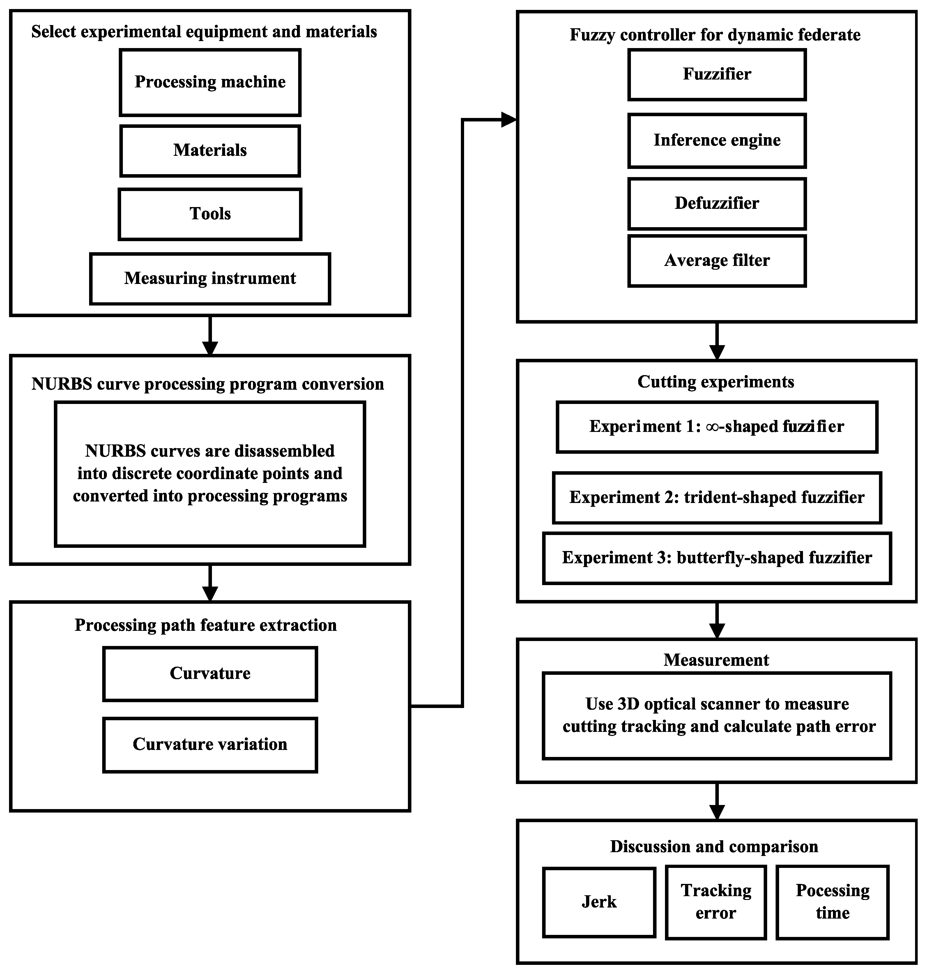
In this study, cutting experiments are performed with three shapes: ∞-shaped, trident-shaped, and butterfly-shaped curves. First, the machining shapes are disassembled into discrete coordinate points and converted into processing programs, next, the machining programs extract features from the curvature and curvature variation. After obtaining the required characteristic values, input those values into the fuzzy controller for feed rate scheduling to obtain the feed rate. Subsequently, an average filter is used to adjust the final feed rate and input the final feed rate in the machining program for actual cutting. Finally, the cutting workpiece is scanned with an optical three-dimensional scanner and the cutting path error is verified. Figure 1 shows the experimental procedure of this study.
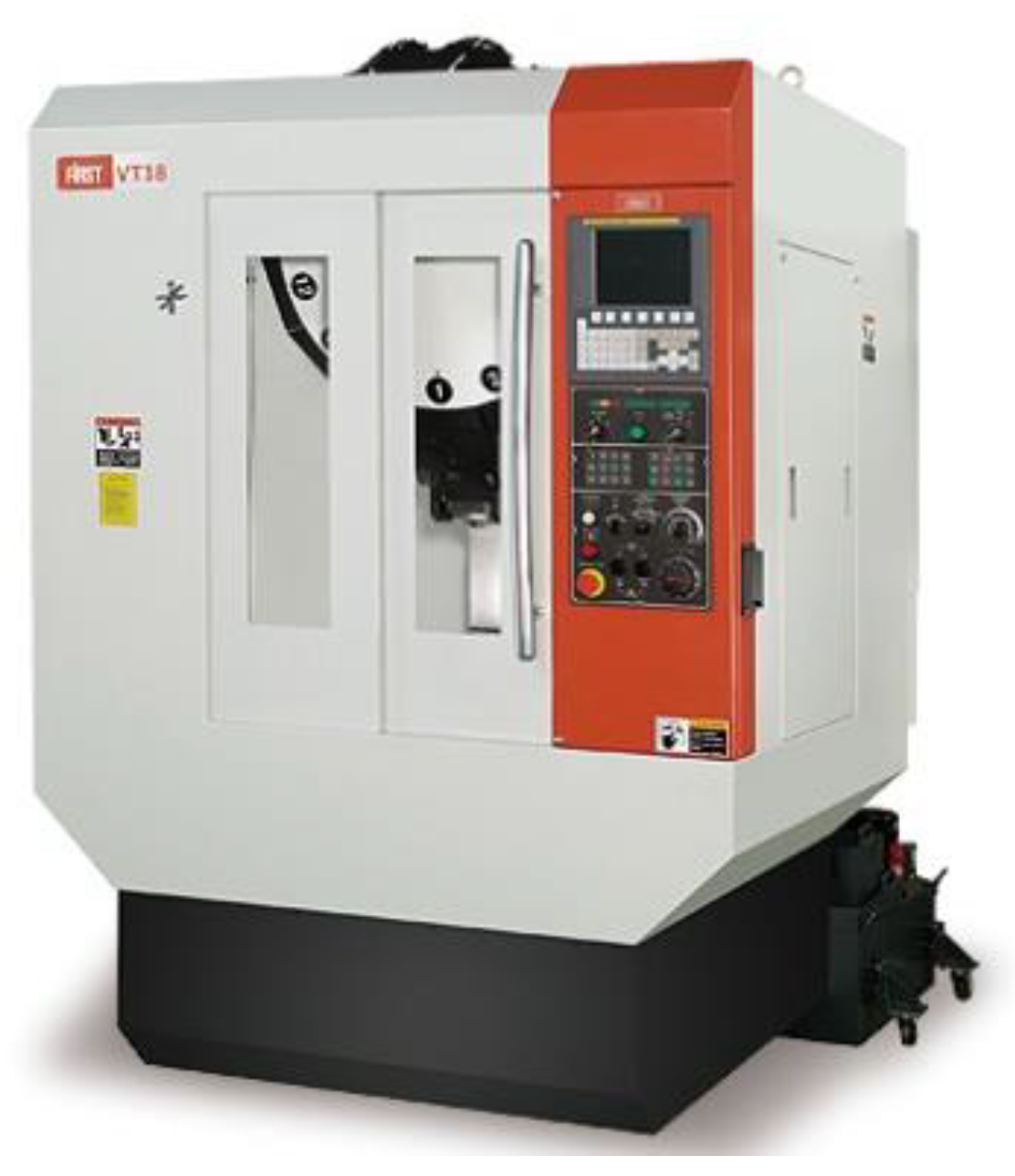
2.1. Processing Machine
2.2. Cutting Material
The 6061 alloy is primarily composed of aluminum, magnesium, and silicon. It has good mechanical properties and welding performance; it is widely used in the manufacture of aircraft structures, boats, and bicycle frames. Moreover, it shows good corrosion resistance; its corrosion resistance is better than that of ordinary carbon steel. Owing to those properties, an aluminum alloy 6061 sample with dimensions of 110 × 100 × 25 is used as the cutting material in the experiment. A cooling cutting fluid is sprayed on the cutting area during processing. Table 2 and Table 3 respectively show the mechanical properties and chemical composition of aluminum alloy 6061.
2.3. Cutting Tool
A tungsten steel ball knife is used as the cutting tool; it produces a V-shaped groove on the workpiece after cutting. The deepest end point of this groove is the tool tip position used to record the tool movement path. Table 4 lists the specifications of the milling cutter.
2.4. Optical Three-Dimensional (3D) Scanner
The optical 3D scanner (ATOS Core, GOM, Braunschweig, Germany) is used to scan the cutting trajectory of the workpiece for verifying the performance of the proposed method. The optical 3D scanner specifications are shown in Table 5.
2.5. Non-Uniform Rational Basis Spline (NURBS) Curve Conversion
NURBS curves were first described by Versprille and were standardized internationally in 1991. According to the Standard for the Exchange of Product Model Data (STEP) promulgated by the International Organization for Standardization (ISO), these curves are the only way to use mathematical expressions as a method to define the geometric shape of a product. NURBS curves have been used often in CAD/CAM. A NURBS curve is defined as follows:
where is the ith control point, is the weight of control point , is the degree basis spline (B-spline), and u = {,....} are knot vectors, and can be defined as a recursive function as follows:
To disassemble a NURBS curve into the coordinate feature points required by the machining code, the precision required for the machining segment must first be defined. Reference [18] mentioned that they use 800 coordinate points to represent the characteristics of the machining segment. To obtain a more precise machining segment, 2000 coordinate points are generated to represent the machining segment for converting into processing programs in this study. All coordinate points can be obtained by simply inputting the series u with an interval of 0.0005 in the NURBS curve function. Finally, all the coordinate points are written into the numerical control code.
2.6. Machining Path Feature Extraction
Many researchers [9,19] showed that the curvature has a great relationship with the machining path error as well as feed rate. Therefore, using a lower feed rate in the machining segment with a larger curvature can effectively reduce the machining path error; however, most scholars used the current curvature as the design method for dynamic feed scheduling. With this method, it is easy to cause excessive acceleration and deceleration in a machining algorithm with uneven curvature distribution. Thus, this study adds the curvature variation as the second condition to enable the dynamic feed scheduling to perform better acceleration and deceleration.
2.6.1. Curvature Calculation
The curvature is a variable that describes the degree of curvature of a curve; at least three coordinate points are required to determine its value. This study is in the XY plane; thus, Figure 3 shows an example of the curvature with three coordinate points (,), (,), and (,).
Assuming this curve is s, its curve equation is given by Equation (4) with six unknowns (,,,,,). Equation (5) can be used to find and that satisfy Equation (6).
This gives Equations (7) and (8), and an inverse matrix is used to find (,,,,,). Then, use Equation (9) to calculate the curvature κ.
2.6.2. Curvature Variation Calculation
After collecting all curvatures, the curvature variation (Dκ) can be calculated using Equation (10). by sliding the window with a window size (WS) of 30. Using a small window size will cause the feed rate to oscillate where the curvature changes greatly. Using a large window size will cause the curvature value to be big and slow down the feed rate. In this study, we use trial and error to determine the window size. After trial and error, we found that setting the window size (WS) to 30 has a smoother curvature value. To enable the fuzzy control for feed rate scheduling to use the maximum curvature in the future as the basis for deceleration, the maximum value is used as the curvature variation.
2.7. Fuzzy Controller for Dynamic Feed Rate Scheduling
The proposed fuzzy control for dynamic feed rate scheduling has two input dimensions: current curvature () and amount of curvature variation (). After fuzzy inference, the current feed rate can be obtained by defuzzification, and all calculated feed rates are input into the average filter to obtain the machining feed rate. Figure 4 shows the architecture of the fuzzy controller for dynamic feed rate.
2.7.1. Fuzzy Rules
A. Fuzzification and membership function
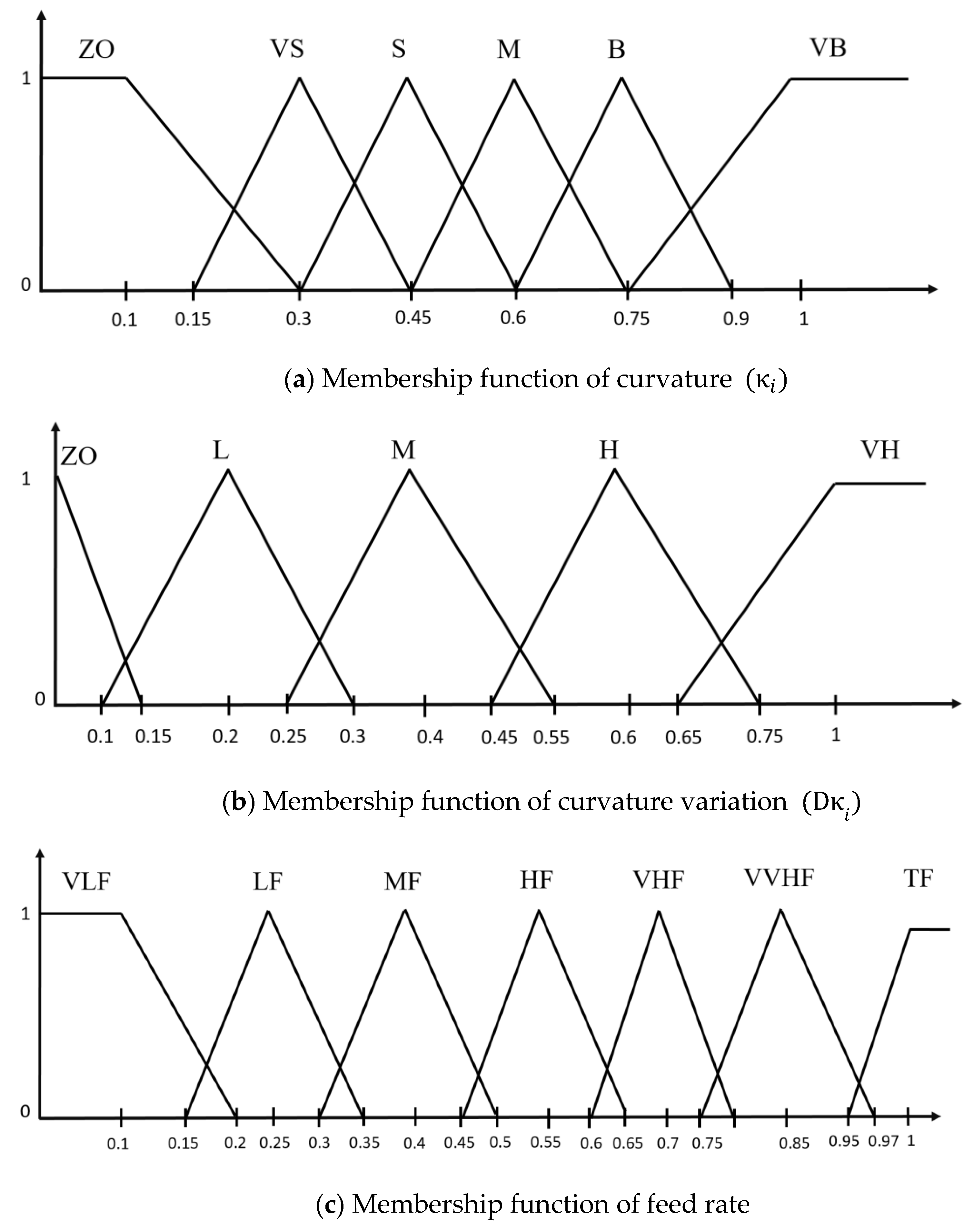
Some common fuzzy membership functions include many different types, such as triangles, trapezoids, and Gaussians. In the past literature, it is pointed out that the use of the Gaussian membership function can obtain better experimental results. Compared with the triangular membership function, the use of the Gaussian membership function requires more computing resources and time. Therefore, in this study, we adopted the triangular membership function to define the input and output membership functions. The first input is the curvature membership function where ZO is the minimum curvature, VS is the very small curvature, S is the small curvature, M is the medium curvature, B is the large curvature, and VB is the maximum curvature. The other input is curvature variation where ZO is the very small change, L is a small change, M is a medium change, H is a large change, and VH is an extremely large change. For the output feed rate membership function, VLF is extremely slow speed, LF is slow speed, MF is medium speed, HF is high speed, VHF is very high speed, VVHF is extremely high speed, and TF is the highest speed. Figure 5 shows the membership functions of the curvature, curvature variation, and feed rate.
When inputting the amount of curvature variation, it is first normalized to the interval [0, 1] based on the maximum and minimum values. After many experiments and adjustments, if the curvature variation remains greater than 3, the curvature variation is represented by the maximum value of 3 and is then normalized. The curvature does not need to be normalized and the output is the feed rate percentage. The current feed rate can be obtained by multiplying by the output with the maximum feed rate, and the user is able to adjust the maximum feed rate to meet the machining requirements.
B. Establishment of fuzzy rules
The two inputs curvature () and curvature variation () designed in the previous section have six and five membership functions, respectively, and the output feed rate has seven membership functions. The tool needs to decelerate early before entering the high-curvature area; for this purpose, a low feed rate is used in the high-curvature area, and acceleration is started after leaving the high-curvature area, as shown in Figure 6. According to this rule, a total of 30 control rules are designed as shown in Table 6.
C. Fuzzy inference and defuzzification
After designing the input and output membership functions and fuzzy control rules, fuzzy inference and defuzzification are needed to calculate the control variable . In this study, the Mamdani fuzzy model is used for fuzzy inference and the control variable derived from the Mamdani fuzzy model is defuzzified to obtain the required precise value. Finally, the center of gravity method is used for defuzzification; the control variable is calculated as follows:
2.7.2. Average Filter
According to the output of the fuzzy controller, a preliminary feed rate value can be obtained. For a simple input graph, the curvature rises and falls stably, the feed rate obtained by the controller is considered relatively stable. By contrast, for a complex input graph, the curvature is unstable causing the output feed rate to oscillate up and down. This study introduces an average filter to eliminate unnecessary oscillations in the feed rate curve. The window size of the average filter () is set to 30. The operation of the average filter is presented as follows:
3. Experimental Results
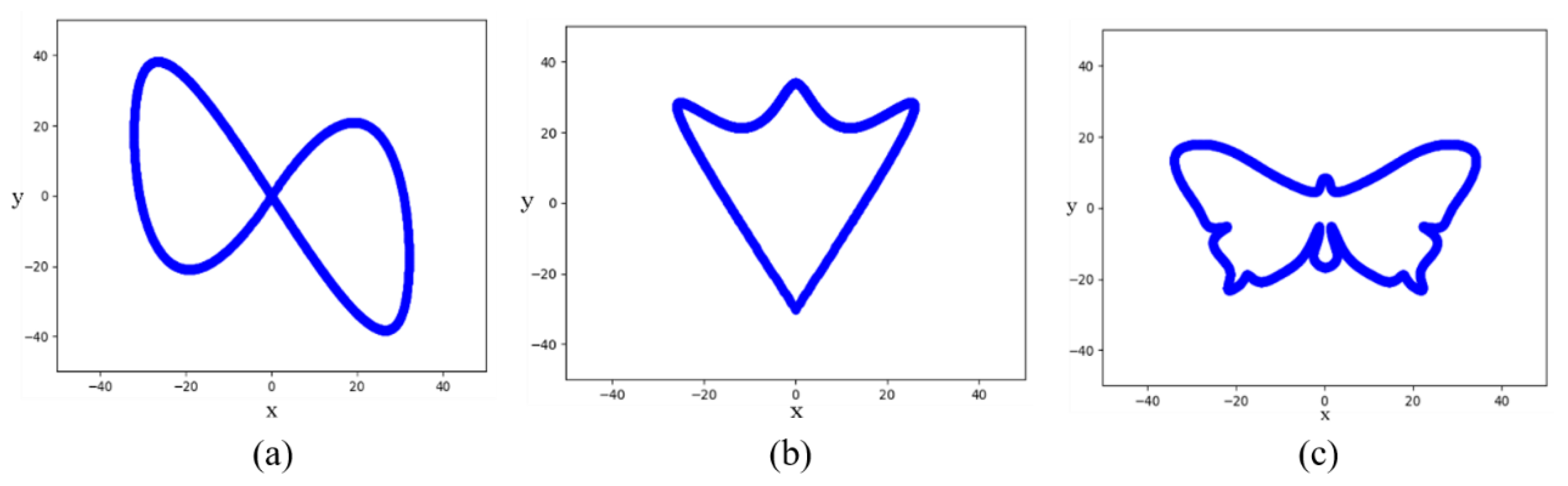
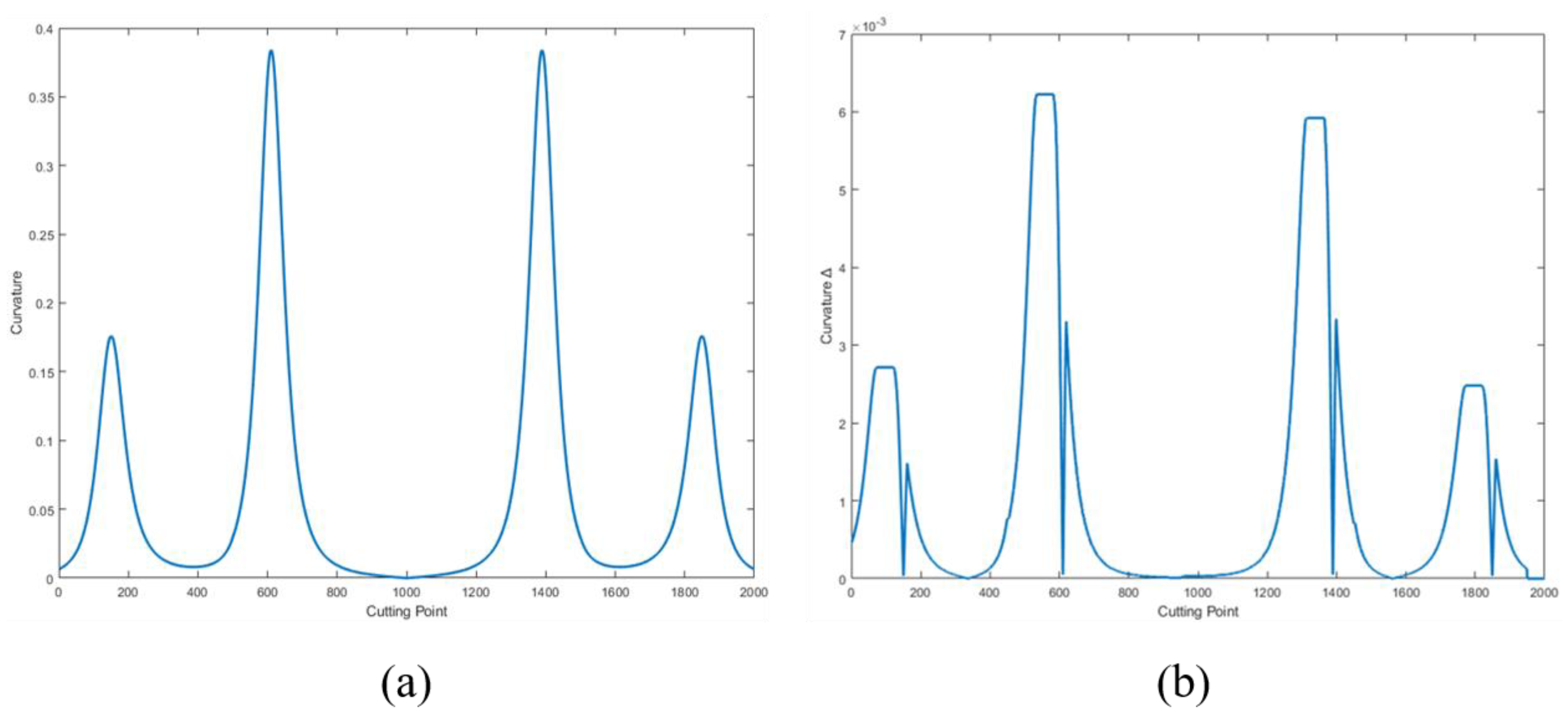
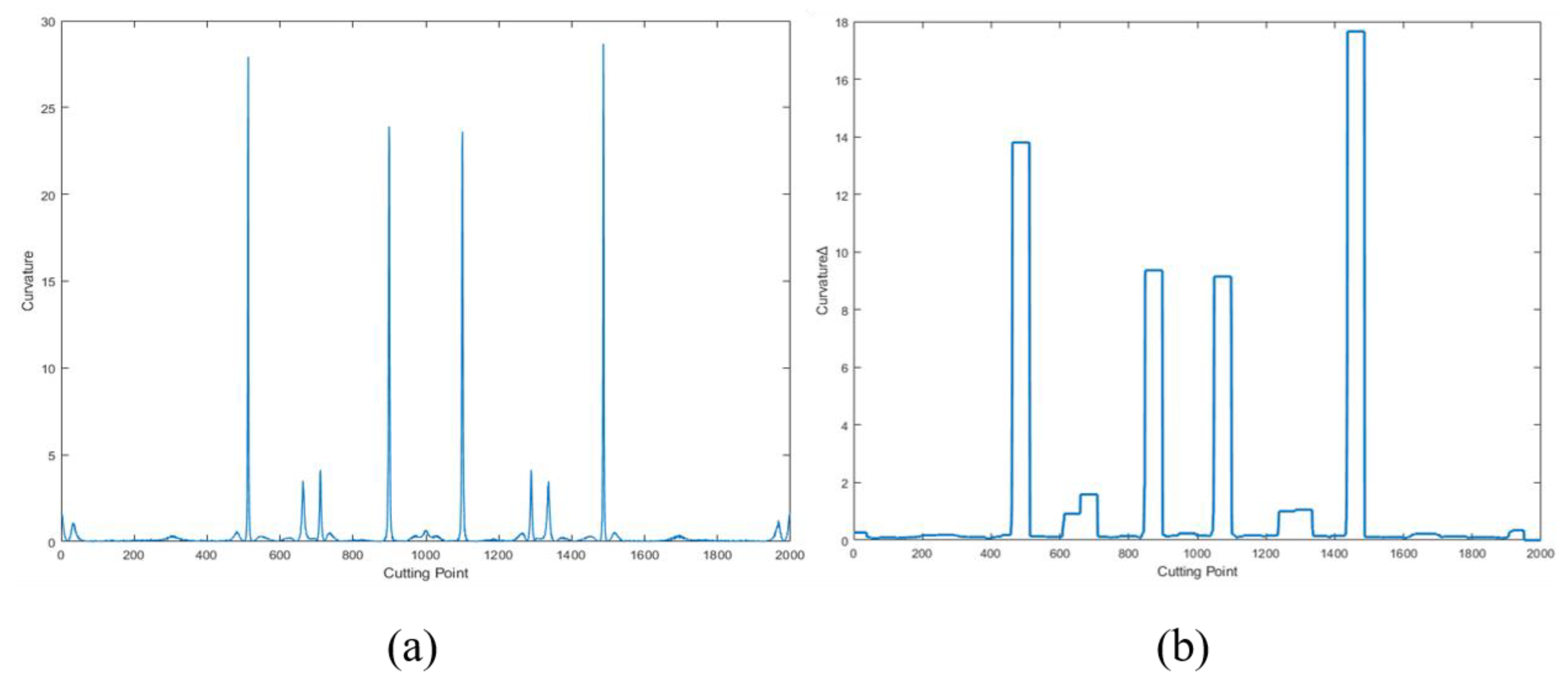
The ∞ shape, trident shape, and butterfly shape graphics [18,20], represented as NURBS graphs in Figure 7a–c, respectively, are used in the cutting experiment. The sizes of those shapes were shrunk to fit into the aluminum workpiece for cutting experiment in addition 2000-point coordinates are generated by a resolution of 0.0005, and the curvature and curvature variation are extracted through the machining path. Figure 8, Figure 9 and Figure 10 show the curvature and curvature variation of the ∞ shape, trident shape, and butterfly shape, respectively.
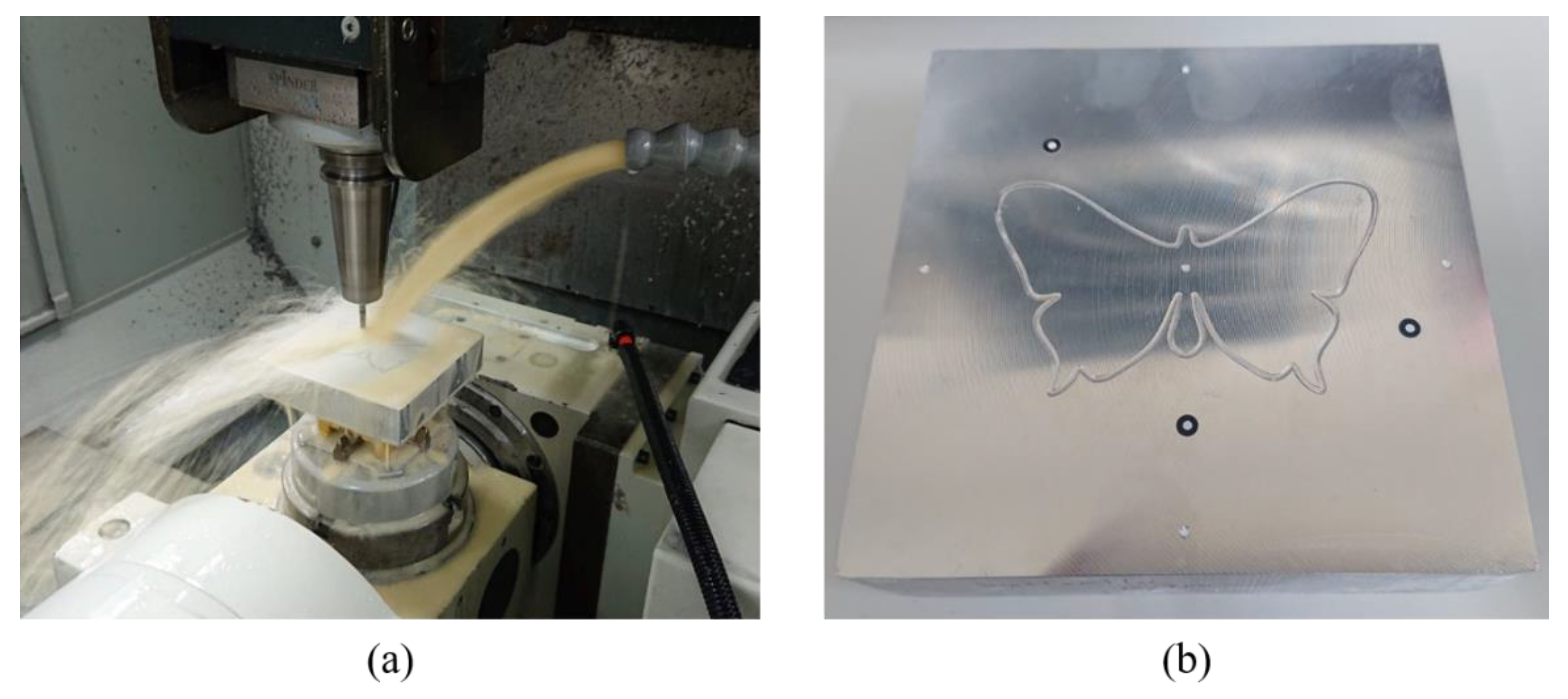
To ensure all the shapes are engraved with the same depth, each aluminum 6061 alloy workpiece will be face-processed before cutting. Furthermore, to prevent the tool from bending, the depth of cut is set to 2 mm. Figure 11a shows the cutting process of an aluminum workpiece, and Figure 11b shows the aluminum workpiece after cutting.
3.1. Optical 3D Scanner Measurement
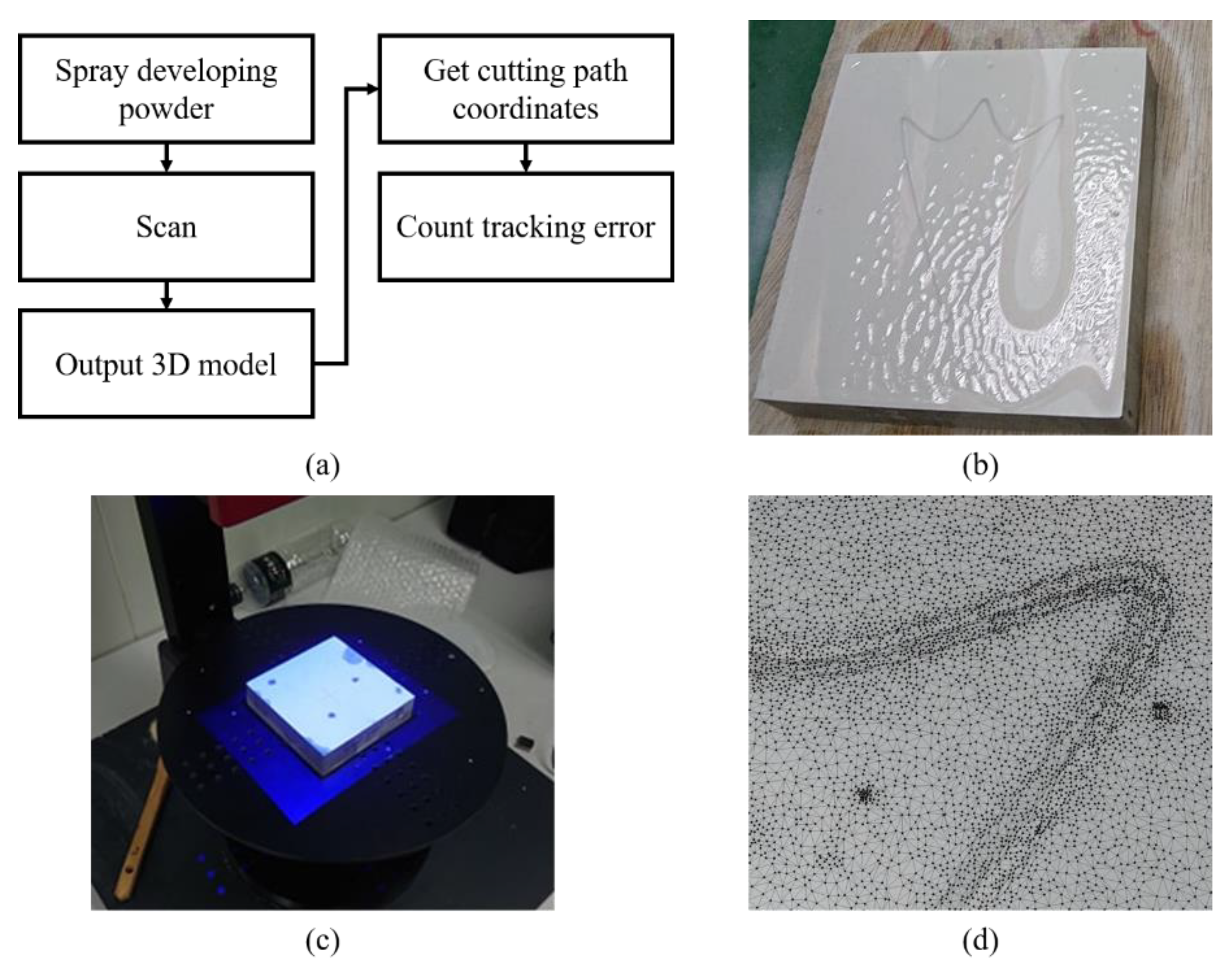
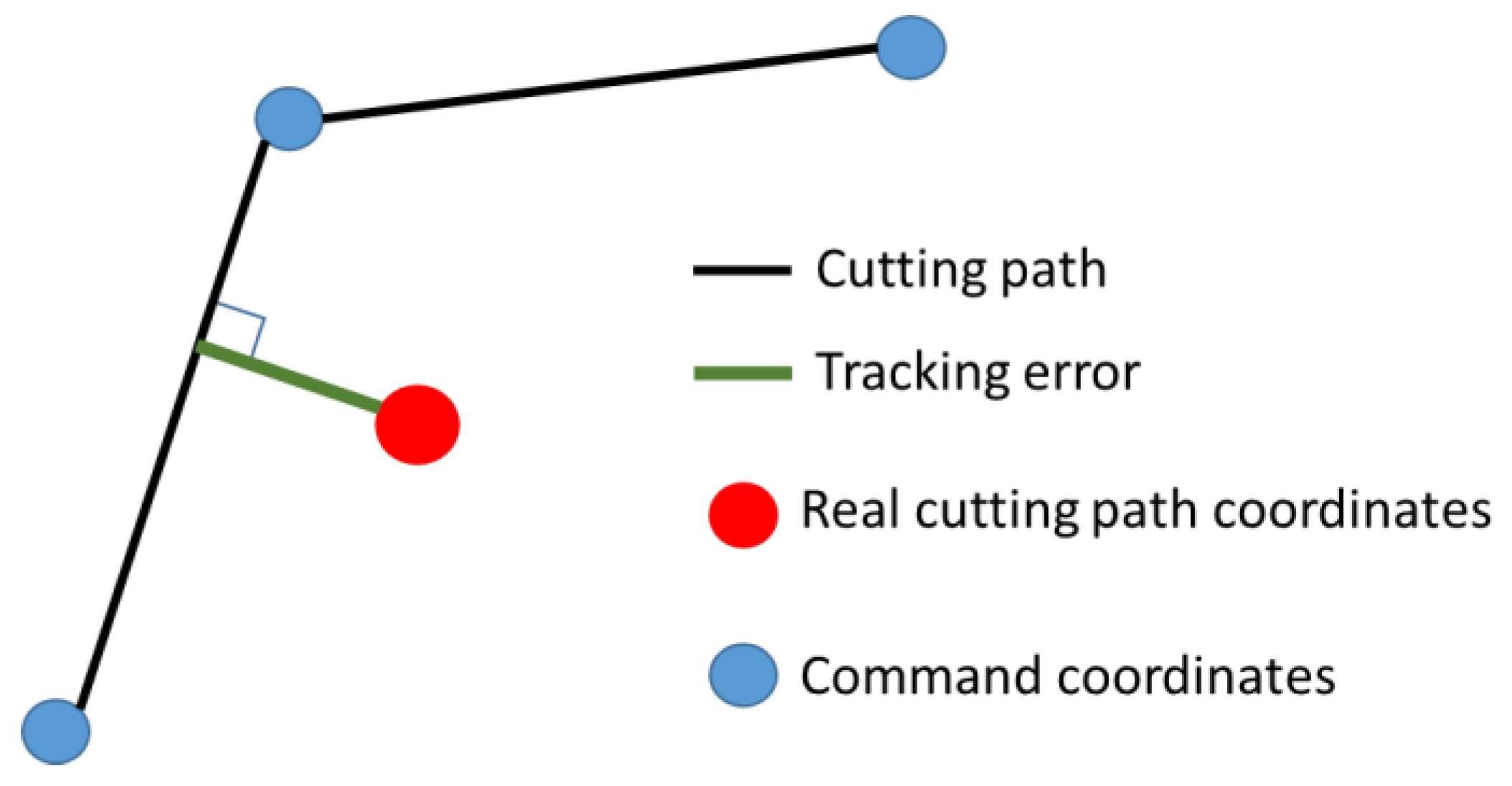
Figure 12a shows a flowchart of optical three-dimensional measurement. First, the surface of the aluminum workpiece can easily refract light; therefore, a developer for measurement must be sprayed before optical measurement, as shown in Figure 12b. Figure 12c shows the scanning with the optical 3D scanner to obtain the geometric features of the workpiece. Figure 13 shows the software output as a binary 3D graphics file. After obtaining the 3D graphics, the deepest coordinate point of the cutting path groove is acquired as the tool tip cutting path. This coordinate is matched to the path of the original machining program, and the shortest distance is calculated as the path error, as shown in Figure 13.
This study performs three experiments. At the same time, three methods proposed by Luan et al. [9], Yeh and Hsu [10], and Giannelli et al. [11] are also adopted to test and compare the results of the proposed method. The lower the tracking error the higher the accuracy and the less machining time the better the machining efficiency is. To performing suitable comparisons, the maximum feed rates, 300, 150, 185, and 58 mm/min, were calculated first according to the methods proposed by scholars before real cutting experiments. Additionally, the properties of the 5-axis CNC processing machine were also taken into consideration during the calculation.
3.2. Experiment 1: Cutting ∞ Shape
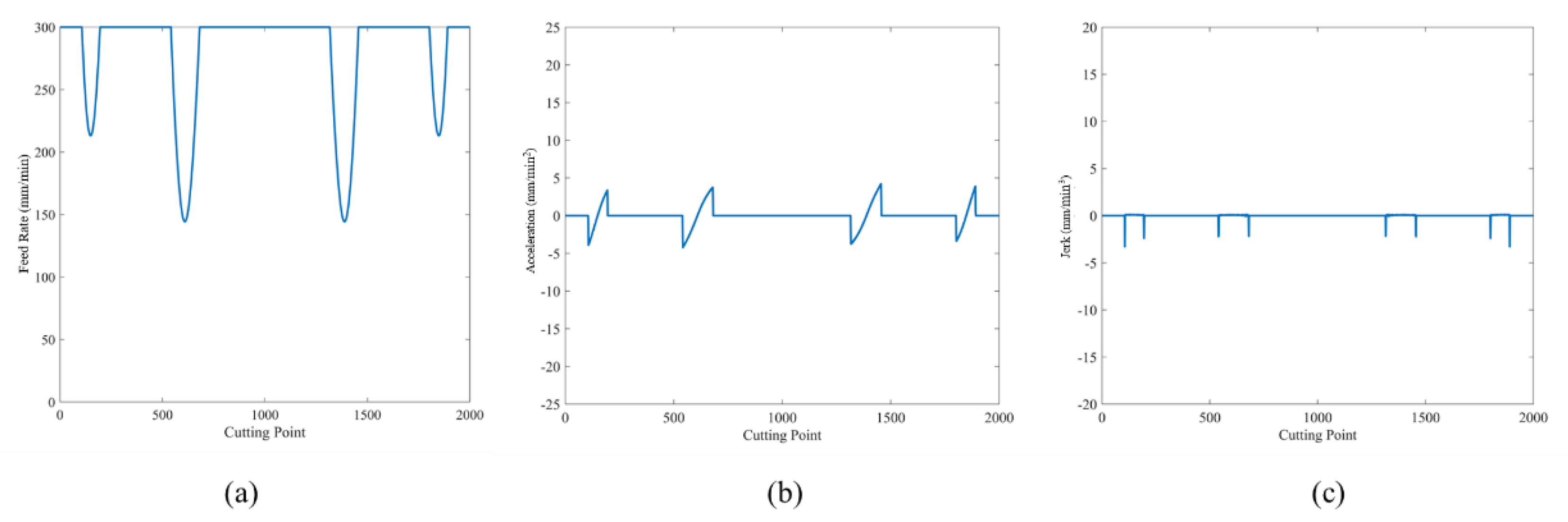
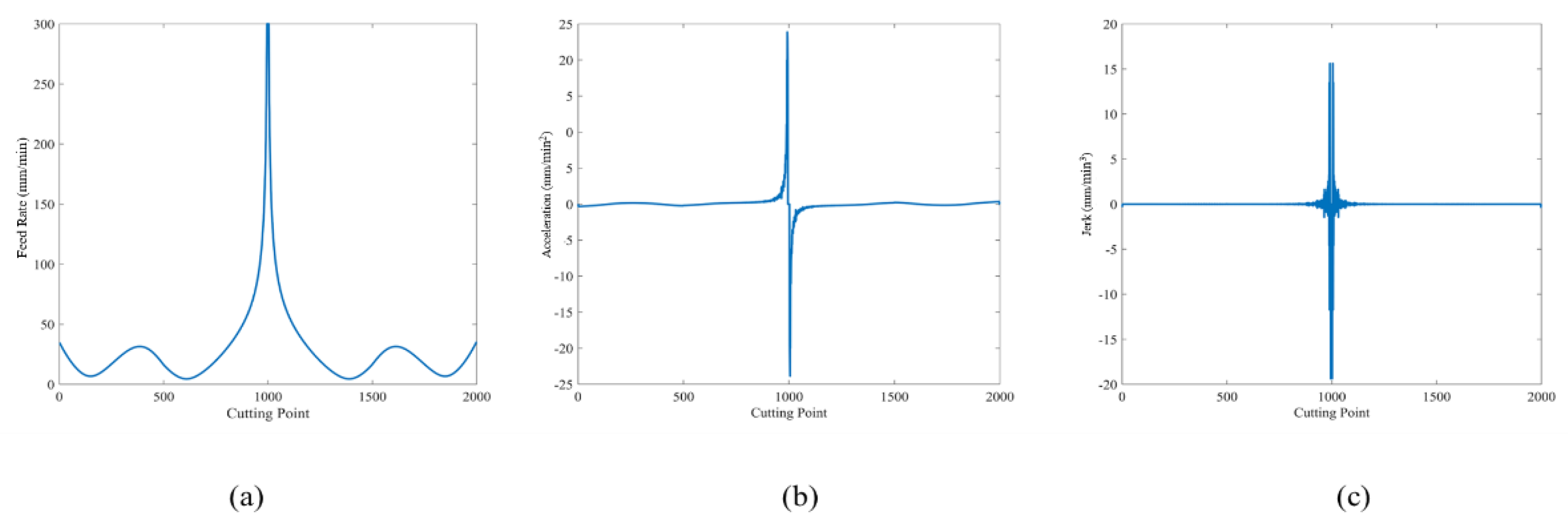
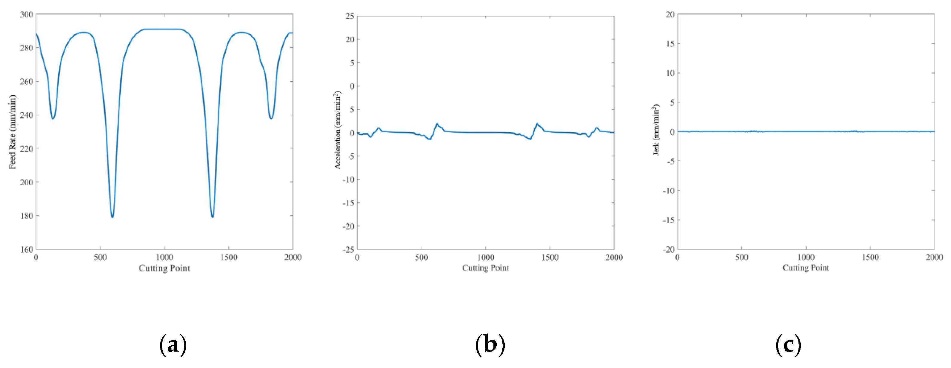
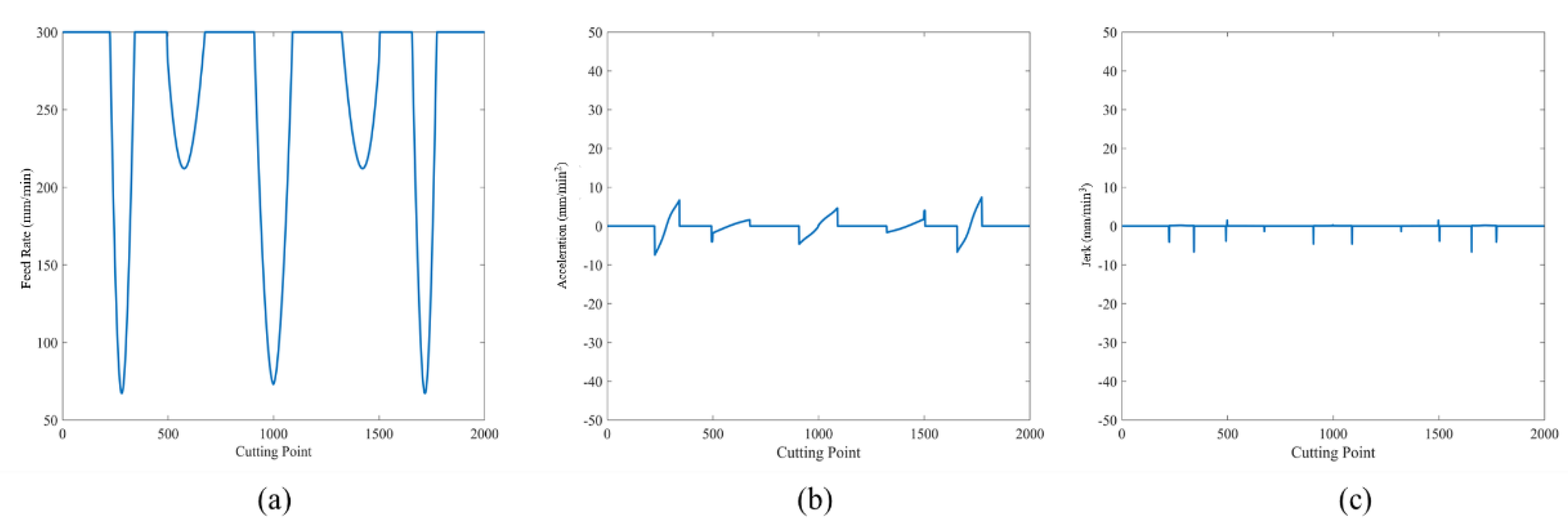
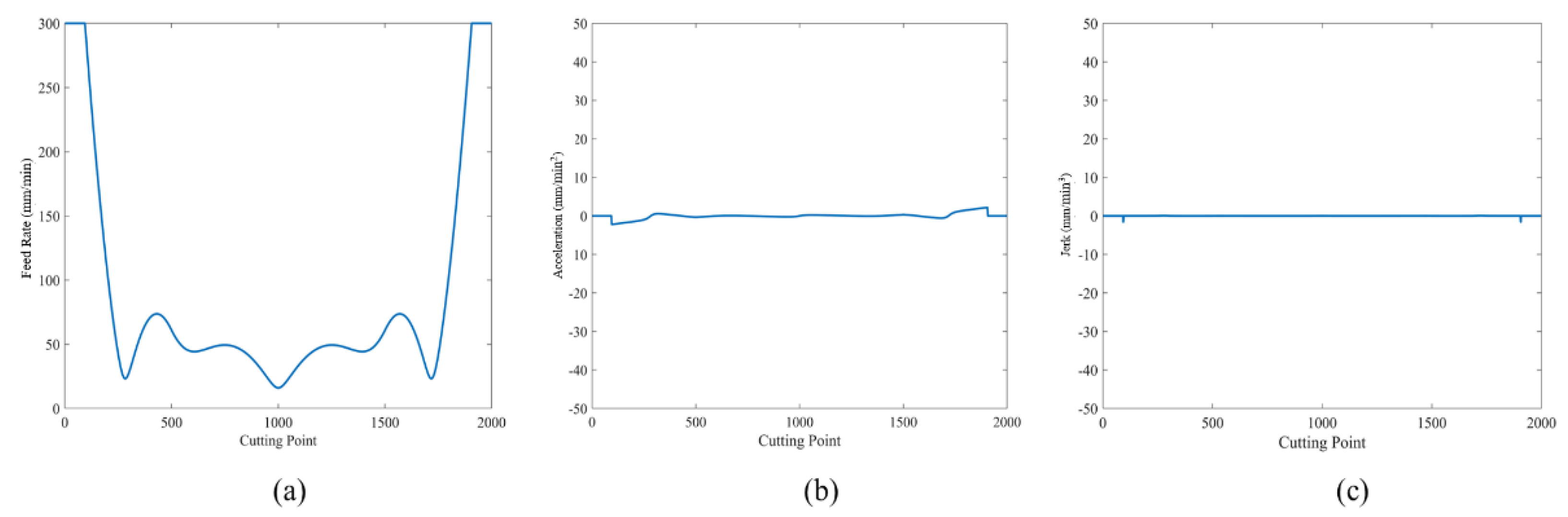
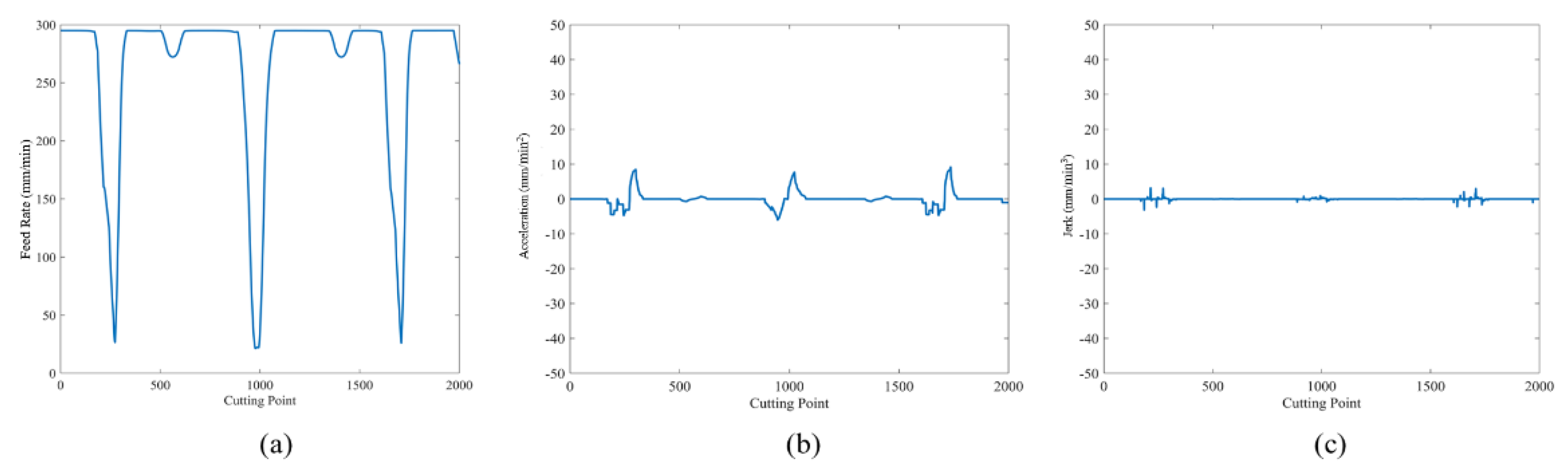
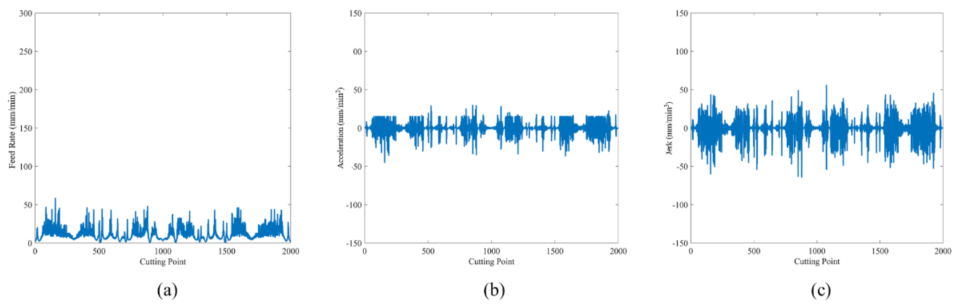
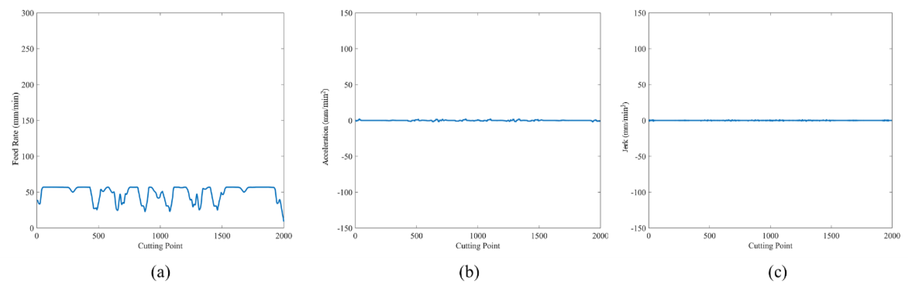
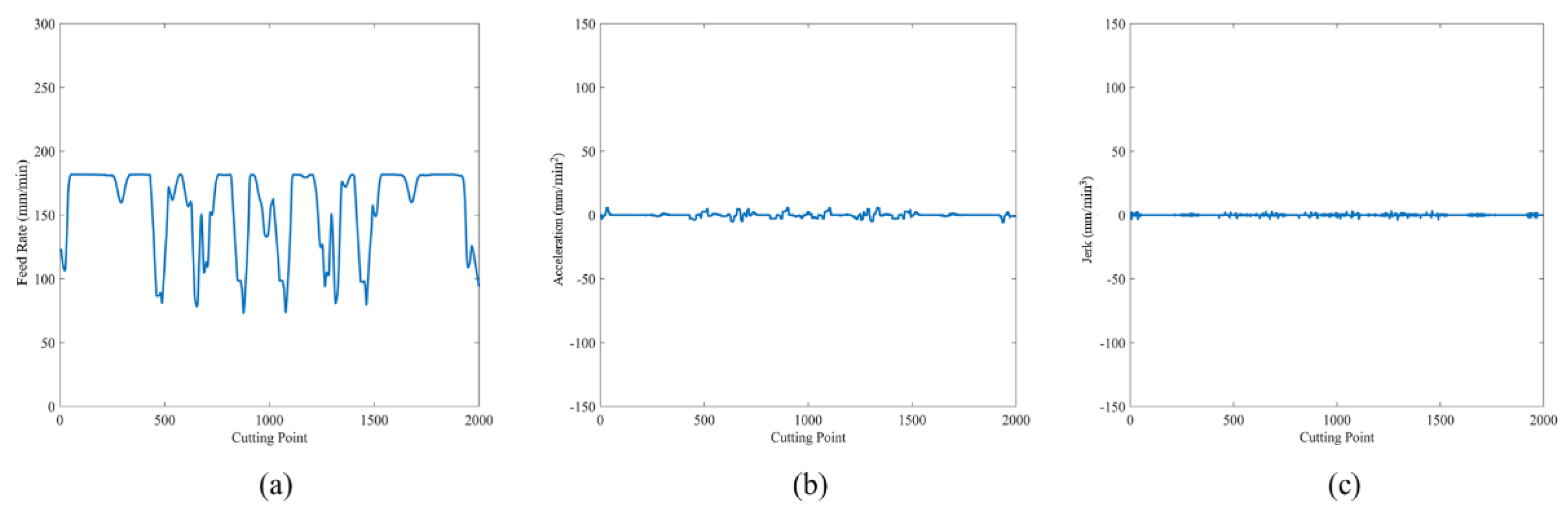
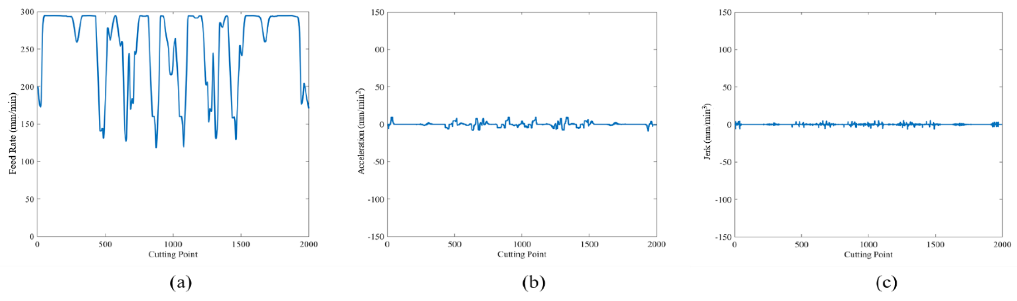
Figure 14, Figure 15, Figure 16 and Figure 17 show the feed rate, acceleration, and jerk of cutting the ∞ shape using the three previous methods and our method, respectively. Table 7 lists the processing time, maximum tracking error, minimum tracking error, average tracking error, and standard deviation. Cutting time indicates that CNC finishes executing the G-code of the machining.
3.3. Experiment 2: Cutting Trident Shape
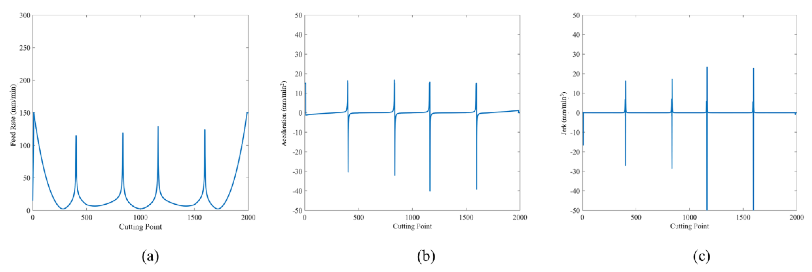
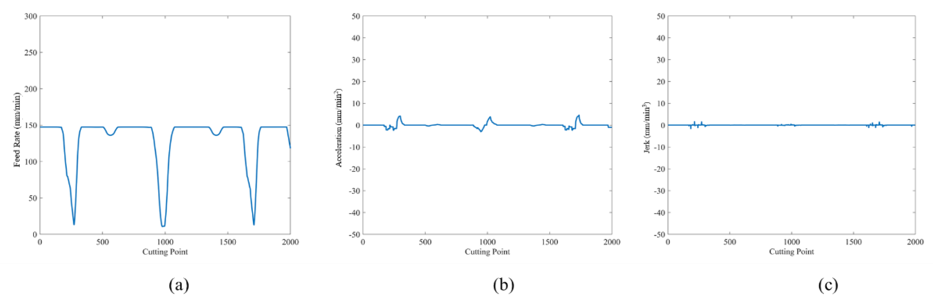
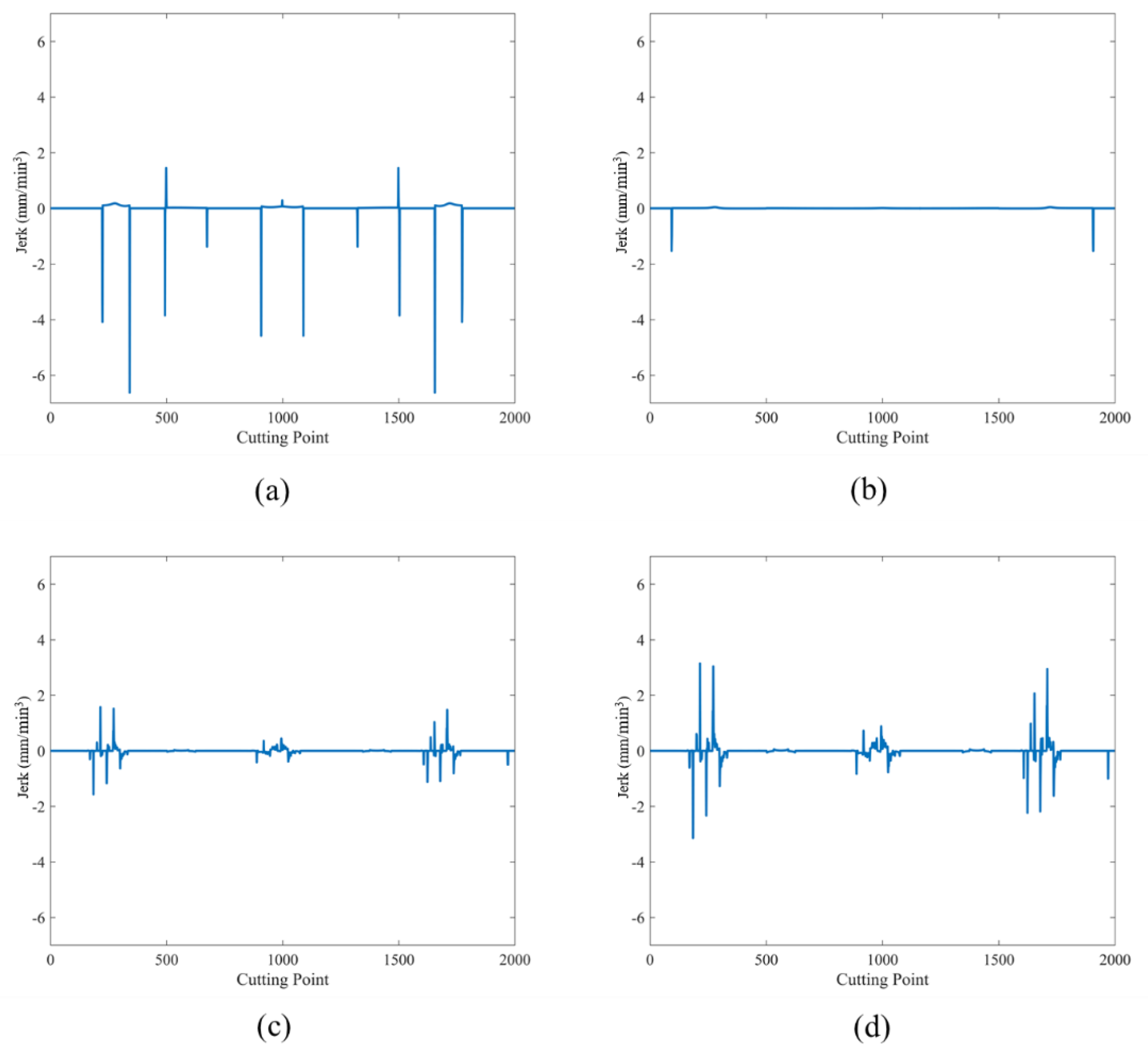
Figure 18, Figure 19 and Figure 20 show the feed rate, acceleration, and jerk when cutting the trident shape using the three previous methods. Figure 21 and Figure 22 show the feed rate, acceleration, and jerk when cutting the trident shapes using our method at maximum feed rates of 150 and 300 mm/min, respectively. Figure 23 shows a comparison of the jerk using the three previous methods and our method. Table 8 lists the processing time, maximum tracking error, minimum tracking error, and average tracking error.
3.4. Experiment 3: Cutting Butterfly Shape
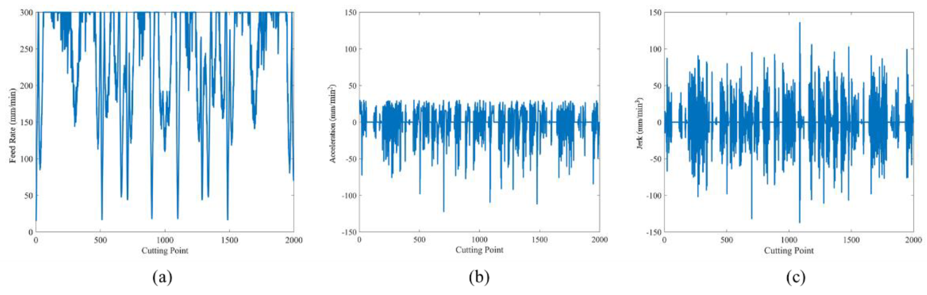
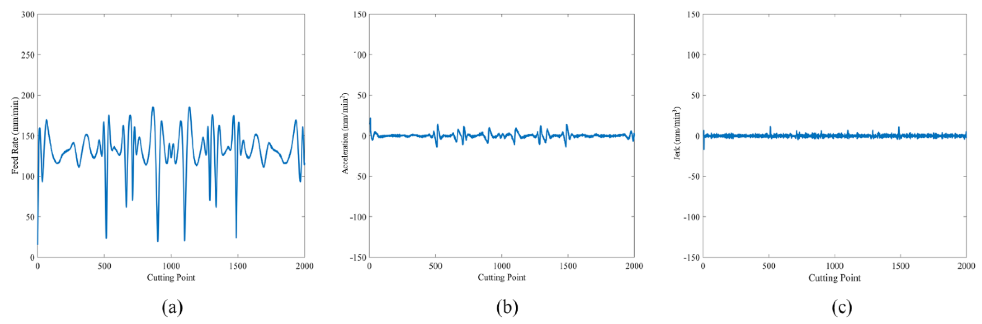
Figure 24, Figure 25 and Figure 26 show the feed rate, acceleration, and jerk when cutting the butterfly shape using the three previous methods. Figure 27, Figure 28 and Figure 29 show the feed rate, acceleration, and jerk when cutting the butterfly shape using our method at maximum feed rates of 58, 185, and 300 mm/min, respectively. Table 9 lists the processing time, maximum tracking error, minimum tracking error, and average tracking error.
4. Discussion
The ∞ shape experimental data indicate that although the method by Giannelli et al. [11] has the largest jerk, the cutting speed is mostly as low as 20 mm/min; therefore, it shows the best tracking error while sacrificing the processing time. The proposed method has the same processing time as the method by Luan et al. [9]. The maximum tracking error is better than 0.041 mm, minimum tracking error is better than 0.006 mm, and average tracking error is better than 0.039 mm. Compared with the method by Yeh and Hsu [10], the maximum tracking error is less than 0.004 mm, minimum tracking error is better than 0.001 mm, and average tracking error is less than 0.005 mm; however, our method requires only half the processing time. In experiment 1, the proposed system increases the cutting accuracy by 41% under the same cutting time; moreover, it decreases the cutting time by 50% under approximative same cutting accuracy (0.023 and 0.028).
The trident shape experimental data prove that the method by Giannelli et al. [11] has the best path error performance, although it somewhat sacrifices the processing time. The proposed method uses a maximum cutting speed of 300 mm/min, in which case its processing time is less than 1 min as with the method by Luan et al. [9], and its maximum tracking error is better than 0.029 mm and average tracking error is better than 0.008 mm. Compared with the method by Yeh and Hsu [10], the average tracking error is poorer than 0.004 mm; yet the processing time is better than 82 s. In experiment 2, the proposed system increases the cutting accuracy by 70% under the approximative same cutting time (46 and 45). Even though our method shows higher average tracking errors in comparison with [10] and [11], the machining time can be saved around 2.8 and 6.5 times, respectively.
The butterfly shape experimental data illustrate that the maximum tracking error of 0.004 mm is better than that of the method by Giannelli et al. [11], average tracking error is better than 0.002 mm, and processing time is half for the same maximum speed. Under the same maximum speed as in the method by Yeh and Hsu [10], the maximum tracking error is better than 0.019 mm, average tracking error is better than 0.003 mm, and processing time is less than 11 s. Our method uses the same maximum speed as the method by Luan et al. [9], and the maximum tracking error is better than 0.029 mm, average tracking error is better than 0.009 mm, and processing time is less than 6 s. In experiment 3, the average tracking error and machining time are all decreasing using the proposed method overall.
5. Conclusions
In this study, fuzzy control is used to productively schedule a reasonable feed rate, and an average filter is used to effectively reduce jerks to avoid excessive impact on the machine. The experimental results prove that our proposed method can effectively shorten the processing time, improve the cutting precision, as well as providing a stable machining which lower standard deviation of tracking error compared with those of three previously proposed methods.
In the future, dynamic feed rate scheduling could be applied to noncontact processing such as laser cutting and 3D printing. The current study only considers the XY plane, so the Z direction can be considered in future studies for dynamic feed rate scheduling to reach an optimal machining. For fuzzy control system, a fuzzy neural network could be implemented to learn the machining parameters of the machine, thus improving the performance of this method.
Author Contributions
Conceptualization, C.-H.L. and C.-J.L.; Methodology, C.-J.L.; Software, C.-H.L.; Data Curation, C.-J.L. and S.-H.W.; Writing-Original Draft Preparation, C.-H.L.; Writing-Review & Editing, C.-J.L.; Supervision, C.-J.L. and S.-H.W.; Funding Acquisition, C.-J.L. and S.-H.W. All authors have read and agreed to the published version of the manuscript.
Funding
This research was funded by the Ministry of Science and Technology of the Republic of China, grant number MOST 110-2634-F-009 -024 and MOST 109-2218-E-005-002.
Institutional Review Board Statement
Not applicable.
Informed Consent Statement
Not applicable.
Data Availability Statement
Data sharing not applicable.
Acknowledgments
The authors would like to thank the support of the Intelligent Manufacturing Research Center (iMRC) from The Featured Areas Research Center Program within the framework of the Higher Education Sprout Project by the Ministry of Education (MOE) in Taiwan.
Conflicts of Interest
The authors declare no conflict of interest.
References
- Saini, S.K.; Pradhan, S.K. Optimization of multi-objective response during CNC turning using Taguchi-fuzzy application. Procedia Eng. 2014, 97, 141–149. [Google Scholar] [CrossRef] [Green Version]
- Gupta, A.; Singh, H.; Aggarwal, A. Taguchi-fuzzy multi output optimization (MOO) in high speed CNC turning of AISI P-20 tool steel. Expert Syst. Appl. 2011, 38, 6822–6828. [Google Scholar] [CrossRef]
- Ulsoy, A.G.; Koren, Y. Control of machining processes. ASME J. Dyn. Syst. Meas. Control. 1993, 115, 301–308. [Google Scholar] [CrossRef]
- Wang, L.; Yuan, X.; Si, H.; Duan, F. Feedrate scheduling method for constant peak cutting force in five-axis flank milling process. Chin. J. Aeronaut. 2020, 33, 2055–2069. [Google Scholar] [CrossRef]
- Kim, S.-J.; Lee, H.-U.; Cho, D.-W. Feedrate scheduling for indexable end milling process based on an improved cutting force model. Int. J. Mach. Tools Manuf. 2006, 46, 1589–1597. [Google Scholar] [CrossRef]
- Lee, H.-U.; Cho, D.-W. Development of a reference cutting force model for rough milling feedrate scheduling using FEM analysis. Int. J. Mach. Tools Manuf. 2007, 47, 158–167. [Google Scholar] [CrossRef]
- He, S.; Ou, D.; Yan, C.; Lee, C.H. A chord error conforming tool path B-spline fitting method for NC machining based on energy minimization and LSPIA. J. Comput. Des. Eng. 2015, 2, 218–232. [Google Scholar] [CrossRef] [Green Version]
- Yeh, S.-S.; Hsu, P.-L. The speed-controlled interpolator for machining parametric curves. Comput. Aided Des. 1999, 31, 349–357. [Google Scholar] [CrossRef]
- Luan, Z.; Jiang, G.; Bai, B.; Zhang, Y.; Mei, X. A feedrate pre-schedule NURBS interpolation method for high-speed machining. In Proceedings of the IEEE ICCA 2010, Xiamen, China, 9–11 June 2010. [Google Scholar]
- Yeh, S.-S.; Hsu, P.-L. Adaptive-feedrate interpolation for parametric curves with a confined chord error. Comput. Aided Des. 2002, 34, 229–237. [Google Scholar] [CrossRef]
- Giannelli, C.; Mugnaini, D.; Sestini, A. C2 continuous time-dependent feedrate scheduling with configurable kinematic constraints. Comput. Aided Geom. Des. 2018, 63, 78–95. [Google Scholar] [CrossRef] [Green Version]
- Zadeh, L.-A. Fuzzy sets. Inf. Control. 1965, 8, 338–353. [Google Scholar] [CrossRef] [Green Version]
- Ratava, J.; Wang, M. High speed constant force milling based on fuzzy controller and BP neural network. Int. J. Adv. Manuf. Technol. 2014, 7, 143–152. [Google Scholar]
- Huang, Y.; Yuan, J. Fuzzy feed rate and cutting speed optimization in turning. Int. J. Control. Autom. 2018, 99, 2081–2092. [Google Scholar]
- Chen, Y.; Zhang, P.; Li, H.B.; Li, P.L.; Yu, Z.Q. Design of PID controller of feed servo-system based on intelligent fuzzy control. Key Eng. Mater. 2016, 639, 1728–1733. [Google Scholar] [CrossRef]
- Miao, Z.; Li, W. A fuzzy system approach of feed rate determination for CNC milling. In Proceedings of the 2009 4th IEEE Conference on Industrial Electronics and Applications, Xi’an, China, 25–27 May 2009. [Google Scholar]
- Liang, M.; Yeap, T.; Hermansyah, A.; Rahmati, S. Fuzzy control of spindle torque for industrial CNC machining. Int. J. Mach. Tools Manuf. 2003, 43, 1497–1508. [Google Scholar] [CrossRef]
- Lin, M.-T.; Tsai, M.-S.; Yau, H.-T. Development of a dynamics-based NURBS interpolator with real-time look-ahead algorithm. Int. J. Mach. Tools Manuf. 2007, 47, 2246–2262. [Google Scholar] [CrossRef]
- Lin, K.-C.; Huang, C.-H.; Tsao, Y.-M.; Wang, J.-C.; Chiu, T.-M. Error dependent variable feedrate interpolation strategy. In Proceedings of the 2010 International Symposium on Computer, Communication, Control and Automation (3CA), Tainan, Taiwan, 5–7 May 2010. [Google Scholar]
- Ni, H.; Zhang, C.; Ji, S.; Hu, T.; Chen, Q.; Liu, Y.; Wang, G. A bidirectional adaptive feedrate scheduling method of NURBS interpolation based on S-shaped ACC/DEC algorithm. IEEE Access 2018, 6, 63794–63812. [Google Scholar] [CrossRef]
Figure 1.
Procedure of fuzzy control for feed rate scheduling.

Figure 2.
Five-axis CNC processing machine used in this study.

Figure 3.
Curvature defined by three coordinate points.

Figure 4.
Architecture of fuzzy controller for dynamic feed rate scheduling.

Figure 5.
Membership functions of (a) curvature, (b) curvature variation, and (c) feed rate.

Figure 6.
Schematic diagram of machining feed rates.

Figure 7.
Experimental cutting graphs: (a) ∞ shape, (b) trident shape, and (c) butterfly shape.

Figure 8.
(a) Curvature and (b) curvature variation of ∞ shape.

Figure 9.
(a) Curvature and (b) curvature variation of trident shape.

Figure 10.
(a) Curvature and (b) curvature variation of butterfly shape.

Figure 11.
(a) Cutting of aluminum workpiece and (b) aluminum workpiece after cutting.

Figure 12.
(a) Flowchart of optical 3D scanner measurement, (b) spraying of developing powder, (c) scanning using optical 3D scanner, and (d) 3D graphics after scanning aluminum workpieces.
Figure 12.
(a) Flowchart of optical 3D scanner measurement, (b) spraying of developing powder, (c) scanning using optical 3D scanner, and (d) 3D graphics after scanning aluminum workpieces.

Figure 13.
Theorical cutting path error calculation.

Figure 14.
Cutting ∞ shape using method by Luan et al. [9]: (a) feed rate, (b) acceleration, and (c) jerk.
Figure 14.
Cutting ∞ shape using method by Luan et al. [9]: (a) feed rate, (b) acceleration, and (c) jerk.

Figure 15.
Cutting ∞ shape using method by Yeh and Hsu [10]: (a) feed rate, (b) acceleration, and (c) jerk.
Figure 15.
Cutting ∞ shape using method by Yeh and Hsu [10]: (a) feed rate, (b) acceleration, and (c) jerk.

Figure 16.
Cutting ∞ shape using method by Giannelli et al. [11]: (a) feed rate, (b) acceleration, and (c) jerk.
Figure 16.
Cutting ∞ shape using method by Giannelli et al. [11]: (a) feed rate, (b) acceleration, and (c) jerk.

Figure 17.
Cutting ∞ shape using our method: (a) feed rate, (b) acceleration, and (c) jerk.

Figure 18.
Cutting trident shape using method by Luan et al. [9]: (a) feed rate, (b) acceleration, and (c) jerk.
Figure 18.
Cutting trident shape using method by Luan et al. [9]: (a) feed rate, (b) acceleration, and (c) jerk.

Figure 19.
Cutting trident shape using method by Yeh and Hsu [10]: (a) feed rate, (b) acceleration, and (c) jerk.
Figure 19.
Cutting trident shape using method by Yeh and Hsu [10]: (a) feed rate, (b) acceleration, and (c) jerk.

Figure 20.
Cutting trident shape using method by Giannelli et al. [11]: (a) feed rate, (b) acceleration, and (c) jerk.
Figure 20.
Cutting trident shape using method by Giannelli et al. [11]: (a) feed rate, (b) acceleration, and (c) jerk.

Figure 21.
Cutting trident shape using our method with maximum feed rate of 150 mm/min: (a) feed rate, (b) acceleration, and (c) jerk.
Figure 21.
Cutting trident shape using our method with maximum feed rate of 150 mm/min: (a) feed rate, (b) acceleration, and (c) jerk.

Figure 22.
Cutting trident shape using our method with maximum feed rate of 300 mm/min: (a) feed rate, (b) acceleration, and (c) jerk.
Figure 22.
Cutting trident shape using our method with maximum feed rate of 300 mm/min: (a) feed rate, (b) acceleration, and (c) jerk.

Figure 23.
Jerk when cutting trident shape using (a) method by Luan et al. [9], (b) method by Yeh and Hsu [10], (c) our method with maximum feed rate of 150 m/min, and (d) our method with maximum feed rate of 300 mm/min.

Figure 24.
Cutting butterfly shape using method by Luan et al. [9]: (a) feed rate, (b) acceleration, and (c) jerk.
Figure 24.
Cutting butterfly shape using method by Luan et al. [9]: (a) feed rate, (b) acceleration, and (c) jerk.

Figure 25.
Cutting butterfly shape using method by Yeh and Hsu [10]: (a) feed rate, (b) acceleration, and (c) jerk.
Figure 25.
Cutting butterfly shape using method by Yeh and Hsu [10]: (a) feed rate, (b) acceleration, and (c) jerk.

Figure 26.
Cutting butterfly shape using method by Giannelli et al. [11]: (a) feed rate, (b) acceleration, and (c) jerk.
Figure 26.
Cutting butterfly shape using method by Giannelli et al. [11]: (a) feed rate, (b) acceleration, and (c) jerk.

Figure 27.
Cutting butterfly shape using our method with maximum feed rate of 58 mm/min: (a) feed rate, (b) acceleration, and (c) jerk.
Figure 27.
Cutting butterfly shape using our method with maximum feed rate of 58 mm/min: (a) feed rate, (b) acceleration, and (c) jerk.

Figure 28.
Cutting butterfly shape using our method with maximum feed rate of 185 mm/min: (a) feed rate, (b) acceleration, and (c) jerk.
Figure 28.
Cutting butterfly shape using our method with maximum feed rate of 185 mm/min: (a) feed rate, (b) acceleration, and (c) jerk.

Figure 29.
Cutting butterfly shapes using our method with maximum feed rate of 300 mm/min: (a) feed rate, (b) acceleration, and (c) jerk.
Figure 29.
Cutting butterfly shapes using our method with maximum feed rate of 300 mm/min: (a) feed rate, (b) acceleration, and (c) jerk.


Table 1.
Parameter settings of the cutting experiments.
| Conditions | Parameters |
|---|---|
| X-Axis | 450 mm |
| Y-Axis | 300 mm |
| Z-Axis | 270 mm |
| Table size | 500 mm × 350 mm |
| Max. spindle speed | 10,000 rpm |
| Three-axis feed rate | X/Y/Z: 48/48/36 m/min |
| Suggested drilling rate | 12 mm/min |
| Max. table loading capacity | 150 kg |
| Controller | FANUC 0i-MD |
Table 2.
Mechanical properties of 6061 aluminum alloy.
| Young’s Modulus | Tensile Strength | Elongation at Break | Poisson’s Ratio | Brinell Scale |
|---|---|---|---|---|
| 68.9 GPa | 124–290 MPa | 12–25% | 0.33 | 30 |
Table 3.
Chemical composition of 6061 aluminum alloy (%).
| Al | Mg | Si | Fe | Cu |
|---|---|---|---|---|
| 9598 | 0.81.2 | 0.40.8 | 00.7 | 0.150.4 |
Table 4.
Specifications of milling cutter.
| Specification Table | Ball-Nose Cutter |
|---|---|
| Overall length (L) | 50 mm |
| Shank diameter (d) | 1.25 mm |
| Teeth number (Teeth) | 2 |
Table 5.
Specifications of optical 3D scanner.
| Scanning Area | Dot Pitch | Measurement Accuracy | Max. Scanning Distance |
|---|---|---|---|
| 200 × 150 mm2 | 0.08 mm | 0.001 mm | 250 mm |
Table 6.
Fuzzy control.
| Curvature Variation | ZO | L | M | H | VH | |
|---|---|---|---|---|---|---|
| Curvature | ||||||
| ZO | TF | TF | VVHF | VVHF | VVHF | |
| VS | VVHF | VVHF | VHF | VHF | VVHF | |
| S | VHF | HF | HF | HF | MF | |
| M | HF | HF | MF | MF | MF | |
| B | MF | LF | LF | VLF | VLF | |
| VB | VLF | VLF | VLF | VLF | VLF | |
Note. ZO = Zero; VS = Very Small; S = Small; M = Medium; B = Big; VB = Very Big; L = Low; M = Medium; H = High; VH = Very High; TF = Extremely Fast Feed; VVHF = Very Very High Feed; VHF = Very High Feed; HF = High Feed; MF = Medium Feed; VLF = Very Low Feed; LF = Low Feed.
Table 7.
Tracking error and processing time of ∞ shape.
| Max Speed (mm/min) | Tracking Error (mm) | Time (s) | ||||
|---|---|---|---|---|---|---|
| MAX | MIN | Average | Standard Deviation | |||
| Luan et al. [9] | 300 | 0.097 | 0.012 | 0.067 | 0.0887 | 62 |
| Yeh and Hsu [10] | 300 | 0.052 | 0.007 | 0.023 | 0.0157 | 122 |
| Giannelli et al. [11] | 300 | 0.012 | 0.001 | 0.005 | 0.0035 | 907 |
| Our method | 300 | 0.056 | 0.006 | 0.028 | 0.0163 | 62 |
Table 8.
Tracking error and processing time for trident shape.
| Max Speed (mm/min) | Tracking Error (mm) | Time (s) | ||||
|---|---|---|---|---|---|---|
| MAX | MIN | Average | Standard Deviation | |||
| Luan et al. [9] | 300 | 0.071 | 0.001 | 0.031 | 0.0194 | 46 |
| Yeh and Hsu [10] | 300 | 0.022 | ~0 | 0.008 | 0.0050 | 127 |
| Giannelli et al. [11] | 150 | 0.006 | 0.001 | 0.004 | 0.0027 | 599 |
| Our method | 300 | 0.042 | ~0 | 0.023 | 0.0120 | 45 |
| 150 | 0.022 | 0.001 | 0.012 | 0.0060 | 92 | |
Table 9.
Tracking error and processing time for butterfly shape.
| Max Speed (mm/min) | Tracking Error (mm) | Time (s) | ||||
|---|---|---|---|---|---|---|
| MAX | MIN | Average | Standard Deviation | |||
| Luan et al. [9] | 300 | 0.09 | ~0 | 0.041 | 0.0194 | 73 |
| Yeh and Hsu [10] | 185 | 0.061 | ~0 | 0.029 | 0.0130 | 120 |
| Giannelli et al. [11] | 58 | 0.028 | ~0 | 0.017 | 0.0048 | 729 |
| Our method | 300 | 0.061 | ~0 | 0.032 | 0.0124 | 67 |
| 185 | 0.042 | ~0 | 0.026 | 0.0102 | 109 | |
| 58 | 0.024 | ~0 | 0.015 | 0.0045 | 360 | |
Publisher’s Note: MDPI stays neutral with regard to jurisdictional claims in published maps and institutional affiliations. |
© 2021 by the authors. Licensee MDPI, Basel, Switzerland. This article is an open access article distributed under the terms and conditions of the Creative Commons Attribution (CC BY) license (https://creativecommons.org/licenses/by/4.0/).
Share and Cite
MDPI and ACS Style
Lin, C.-J.; Lin, C.-H.; Wang, S.-H. Using Fuzzy Control for Feed Rate Scheduling of Computer Numerical Control Machine Tools. Appl. Sci. 2021, 11, 4701. https://0-doi-org.brum.beds.ac.uk/10.3390/app11104701
AMA Style
Lin C-J, Lin C-H, Wang S-H. Using Fuzzy Control for Feed Rate Scheduling of Computer Numerical Control Machine Tools. Applied Sciences. 2021; 11(10):4701. https://0-doi-org.brum.beds.ac.uk/10.3390/app11104701
Chicago/Turabian StyleLin, Cheng-Jian, Chun-Hui Lin, and Shyh-Hau Wang. 2021. "Using Fuzzy Control for Feed Rate Scheduling of Computer Numerical Control Machine Tools" Applied Sciences 11, no. 10: 4701. https://0-doi-org.brum.beds.ac.uk/10.3390/app11104701
Note that from the first issue of 2016, this journal uses article numbers instead of page numbers. See further details here.