A Novel Maneuver-Based Driving Envelope Generation Approach for Driving Safety Assessment

Abstract

It is of utmost importance for advanced driver assistance systems to evaluate the risk of the current situation and make continuous decisions about what kind of evasive maneuver can be initiated. The purpose of this paper is to establish efficient indicators to evaluate the risk of candidate driving maneuvers for a human-in-the-loop vehicle. A novel safe driving envelope generation method is proposed, which takes various constraints into consideration, including the human operation, vehicle motion limits, and collision avoidance with road boundary and obstacles. The efficiency of the proposed method is validated by simulation experiments and real vehicle tests. The results show that the feasibility of candidate driving maneuvers can be efficiently determined by computing the driving envelope, and the proposed driving envelope method can be easily implemented for real-time applications.

1. Introduction

The advanced driver assistance systems (ADAS) are expected to reduce the risk of accidents and enhance driving comfort. The driving states can be classified into five types: normal driving state, warning state, collision avoidable state, collision inevitable state, and post-collision state. With a human-in-the-loop, it is necessary to establish safety indicators for situation assessment to determine whether the vehicle is in a safe state and whether the driver can avoid potential collisions.

Generally, the driving situation assessment modular estimates the current driving state, predicts the future driving state, and evaluates the collision risk. The single threat metric includes time-related metrics, acceleration-related metrics, and distance-related metrics, etc. Given the current speed of the host vehicle, the Inter-Vehicle-Time (IVT) indicates the time required for the host vehicle to travel the relative distance to the obstacle [1]. The time-to-collision (TTC) denotes the collision time under the assumption that the vehicle will follow a specific trajectory in the future time-domain [2]. Time-to Maneuver (TTM) is the remaining time to avoid a collision by a specific driving maneuver, such as Time-to-Brake (TTB), Time-to-Steer (TTS), and Time-to-Kickdown (TTK) [3,4]. The Brake Threat Number (BTN) and the Steering Threat Number (STN) are acceleration-related metrics introduced in [5,6]. The STN is used to evaluate the risk of the steering maneuver to avoid a collision. The BTN is an indicator for evaluating the risk of braking to avoid a collision. The minimum safe distance in [7] is calculated under the assumption that the leading vehicle will maintain a constant deceleration until it comes to a stop, and the host vehicle starts to brake at a constant deceleration after reaction time. The minimal safe distance (MSD) is the safe distance required for two vehicles to keep minimal safety [8]. The Minimum Longitudinal Safety Spacing (MLSS) represents the safe distance to start a lane-change maneuver [9]. However, the above methods have not considered the current input of the driver. Due to the driving limits and driving comfort, the curvature of the evasive path should have an upper bound.

In some works, path planning methods are used to determine whether there is a safe obstacle avoidance trajectory. In [10,11,12,13,14,15], the motion planner generates a bundle of candidate trajectories, and the safety of each trajectory is determined by collision detection. In [16,17,18,19,20], the handling envelope and the environmental envelope at each time step are taken into account. Whether a safe trajectory exists or not is identified by solving the optimization problem of trajectory generation. However, these methods consume massive computing resources.

For a human-in-the-loop system, the human and the machine are complicatedly coupled. The driver’s input and the vehicle’s driving safety need to be considered at the same time. The Inevitable Collision State (ICS) is defined as a state that ultimately ends in a collision, regardless of what the input is selected [21,22,23]. In [24], the reachable occupancy without collision utilizing the concept of ICS is calculated at discrete time steps. However, determining the set of ICS is computationally expensive. Owing to the consumption of computing resources, it is difficult to apply ICS in real-time, and the time horizon is often very short. In [25,26,27], a kind of reachable set is mentioned, where the current input of the driver can be considered. The data-driven reachable set is built to represent the probability distribution of the future trajectories considering individual driver steering behavior. The probability distribution of future position is highly related to the curvature of the road. The data-driven method needs to learn the distribution on roads with different curvatures. The extreme trajectory bound for obstacle avoidance is not generated, and the existence of collision avoidance trajectories is determined by checking the collision area of the obstacles and the reachable set of the ego vehicle. Inspired by their work, we propose a driving envelope for a human-in-the-loop vehicle considering the various constraints including human operation, vehicle motion limits, and collision avoidance with road boundaries and obstacles.

The main contributions of our work are two-fold. First, the safe distance considering uncertainty for collision avoidance with obstacles is derived. The lateral motion and the longitudinal motion are considered. The extreme boundary trajectories for collision avoidance are obtained based on the derived safe distance. Second, a novel driving envelope is proposed. The driving envelope considers the constraints including steering input of the driver, vehicle motion limitation, the boundary of road, and the safe distance for collision avoidance. Using the proposed driving envelope, the safety and the intervention time of candidate driving maneuvers can be determined. Motion planning algorithm can be applied considering the proposed driving envelope.

The safe distance in this paper is inspired by the MLSS [9], which is the safe distance to start a lane-change maneuver, the safe distance during the lane-change process is not derived. In this paper, the safe distances during the lane-change process and for the lane-change abortion are derived. The driving envelope in this paper is different from that in [27], where the sub-reachable-set generation method did not consider the collision avoidance behavior with obstacles on the road. In this paper, the collision avoidance maneuver is considered for the driving envelope generation method. The proposed driving envelope in this paper is also different from that in [16,17,18,19,20], where the environmental driving envelope is the unoccupied area at each prediction step. In the above papers, whether safe trajectories exist or not is identified by solving the optimization problem of trajectory generation. The driving envelope proposed in this paper is the non-collision area during the whole time domain of lane-change maneuver and lane-change abortion maneuver. The existence of non-collision trajectories can be identified based on the proposed driving envelope conveniently. In the future, with the help of V2X technology [28,29], the uncertainty of perception and prediction will be reduced, and the driving envelope will be more reliable. Furthermore, the proposed driving envelope can be used for guiding the search of an underlying planning algorithm to find a solution and determining the time for intervention.

The remainder of this paper is organized as follows. The motion constraints for human-in-the-loop vehicles are introduced in Section 2. The driving envelope for candidate maneuvers is described in Section 3. The applications of the proposed driving envelope are discussed in Section 4. The experiment results and the discussions are shown in Section 5. The conclusions are drawn in Section 6.

2. The Motion Constraints

The motion of a vehicle is constrained by the vehicle kinematic limitation, and should not collide with road boundary or obstacles.

2.1. The Constraint of Vehicle Kinematic

The maximally allowed acceleration is limited by the friction force, which can be represented by a friction circle on a g-g diagram [30]. Factors including weight transfer, bank and grade of the road will affect the shape of the friction circle. These factors can be considered to obtain accurate vehicle dynamic models under different road conditions [31]. The permissible speed ${\mathit{v}}_{\mathit{l}\mathit{i}\mathit{m}}$ is limited by the road curvature $\kappa$ and the maximum allowed speed ${\mathit{v}}_{\mathit{m}\mathit{a}\mathit{x}}$. The longitudinal and lateral motion in the reference frame is limited by the ability of accelerating and decelerating and the friction force.

$${\mathit{v}}_{\mathit{l}\mathit{i}\mathit{m}}=\mathit{m}\mathit{i}\mathit{n}(\sqrt{\frac{{\mathit{a}}_{\mathit{l}\mathit{a}\mathit{t}}}{\kappa }},{\mathit{v}}_{\mathit{m}\mathit{a}\mathit{x}})$$

(1a)

$$\sqrt{{\mathit{a}}_{\mathit{l}\mathit{o}\mathit{n}}^2+{\mathit{a}}_{\mathit{l}\mathit{a}\mathit{t}}^2}⩽{\mathit{a}}_{max}$$

(1b)

$${\mathit{a}}_{min,\mathit{l}\mathit{o}\mathit{n}}\le {\mathit{a}}_{\mathit{l}\mathit{o}\mathit{n}}\le {\mathit{a}}_{max,\mathit{l}\mathit{o}\mathit{n}}$$

(1c)

$$-{\mathit{a}}_{max,\mathit{l}\mathit{a}\mathit{t}}\le {\mathit{a}}_{\mathit{l}\mathit{a}\mathit{t}}\le {\mathit{a}}_{max,\mathit{l}\mathit{a}\mathit{t}}$$

(1d)

where ${\mathit{a}}_{\mathit{l}\mathit{a}\mathit{t}}$ is the lateral acceleration, ${\mathit{a}}_{\mathit{l}\mathit{o}\mathit{n}}$ is the longitudinal acceleration, ${\mathit{a}}_{max,\mathit{l}\mathit{o}\mathit{n}}$ represents the maximum longitudinal acceleration, ${\mathit{a}}_{min,\mathit{l}\mathit{o}\mathit{n}}$ represents minimum longitudinal acceleration, ${\mathit{a}}_{max,\mathit{l}\mathit{a}\mathit{t}}$ represents the maximum allowed lateral acceleration.

2.2. The Evasive Motion Model

Motion planning in a dynamic environment involves many aspects, such as collision avoidance, the drivability of the planned trajectory, and the motion of the other traffic participants in the future, etc. In [32], the minimum distance required for avoiding the front dynamic obstacle was analyzed. However, the paper only considered avoiding obstacles with a constant steering angle. The constraints on the terminal state of the host vehicle after avoiding obstacles have not been considered. It is not guaranteed to adjust the state of the vehicle in the lane boundary after a collision-avoidance maneuver. In a real traffic scenario, after an evasive maneuver or lane-change maneuver, the vehicle should adjust the heading angle to avoid collision with the road boundary. In this paper, we utilize an evasive motion model in [9]. The motion of the host vehicle is decomposed into lateral movement and longitudinal movement in the reference frame. The lateral motion model in the reference frame is described as follows.

$$\begin{array}{cc}\hfill {\mathit{a}}_{\mathit{l}\mathit{a}\mathit{t}}\left(\mathit{t}\right)=& \left\{\begin{array}{c}\frac{2\pi \mathit{H}}{{\mathit{t}}_{\mathit{l}\mathit{a}\mathit{t}}^2}sin\left(\frac{2\pi }{{\mathit{t}}_{\mathit{l}\mathit{a}\mathit{t}}}\mathit{t}\right),\mathit{t}\le {\mathit{t}}_{\mathit{l}\mathit{a}\mathit{t}}\hfill \\ 0,\mathrm{otherwise}\hfill \end{array}\right.\hfill \end{array}$$

(2a)

$$\begin{array}{cc}\hfill {\mathit{v}}_{\mathit{l}\mathit{a}\mathit{t}}\left(\mathit{t}\right)=& \left\{\begin{array}{c}-\frac{\mathit{H}}{{\mathit{t}}_{\mathit{l}\mathit{a}\mathit{t}}}cos\left(\frac{2\pi }{{\mathit{t}}_{\mathit{l}\mathit{a}\mathit{t}}}\mathit{t}\right)+\mathit{H}/{\mathit{t}}_{\mathit{l}\mathit{a}\mathit{t}},\mathit{t}\le {\mathit{t}}_{\mathit{l}\mathit{a}\mathit{t}}\hfill \\ 0,\mathrm{otherwise}\hfill \end{array}\right.\hfill \end{array}$$

(2b)

$$\begin{array}{cc}\hfill \mathit{y}\left(\mathit{t}\right)=& -\frac{\mathit{H}}{2\pi }sin\left(\frac{2\pi }{{\mathit{t}}_{\mathit{l}\mathit{a}\mathit{t}}}\mathit{t}\right)+\frac{\mathit{H}}{{\mathit{t}}_{\mathit{l}\mathit{a}\mathit{t}}}\mathit{t}+{\mathit{y}}_0\hfill \end{array}$$

(2c)

$$\begin{array}{cc}\hfill \mathit{H}=& {\mathit{y}}_{\mathit{t}\mathit{a}\mathit{r}\mathit{g}\mathit{e}\mathit{t}}-{\mathit{y}}_0\hfill \end{array}$$

(2d)

where ${\mathit{a}}_{\mathit{l}\mathit{a}\mathit{t}}$ is the lateral acceleration in the reference frame, ${\mathit{t}}_{\mathit{l}\mathit{a}\mathit{t}}$ is the required total time to finish the lateral motion, H is the total lateral moving distance of the evasive maneuver, ${\mathit{y}}_0$ is the starting lateral position in the reference frame, ${\mathit{y}}_{\mathit{t}\mathit{a}\mathit{r}\mathit{g}\mathit{e}\mathit{t}}$ is the terminal lateral position in the reference frame. As mentioned in [33], the comfort zone of lateral acceleration should be within $\mathit{a}\in \left[-2,2\right]$. The longitudinal motion model in the reference frame can be defined as follows.

$$\begin{array}{cc}\hfill {\mathit{x}}_{\mathit{l}\mathit{o}\mathit{n}}\left(\mathit{t}\right)=& {\mathit{v}}_{\mathit{l}\mathit{o}\mathit{n}}\left(0\right)\mathit{t}+\frac{1}{2}\mathit{a}{\mathit{t}}^2\hfill \end{array}$$

(3a)

$$\begin{array}{cc}\hfill {\mathit{v}}_{\mathit{l}\mathit{o}\mathit{n}}\left(\mathit{t}\right)=& {\mathit{v}}_{\mathit{l}\mathit{o}\mathit{n}}\left(0\right)+\mathit{a}\mathit{t}\hfill \end{array}$$

(3b)

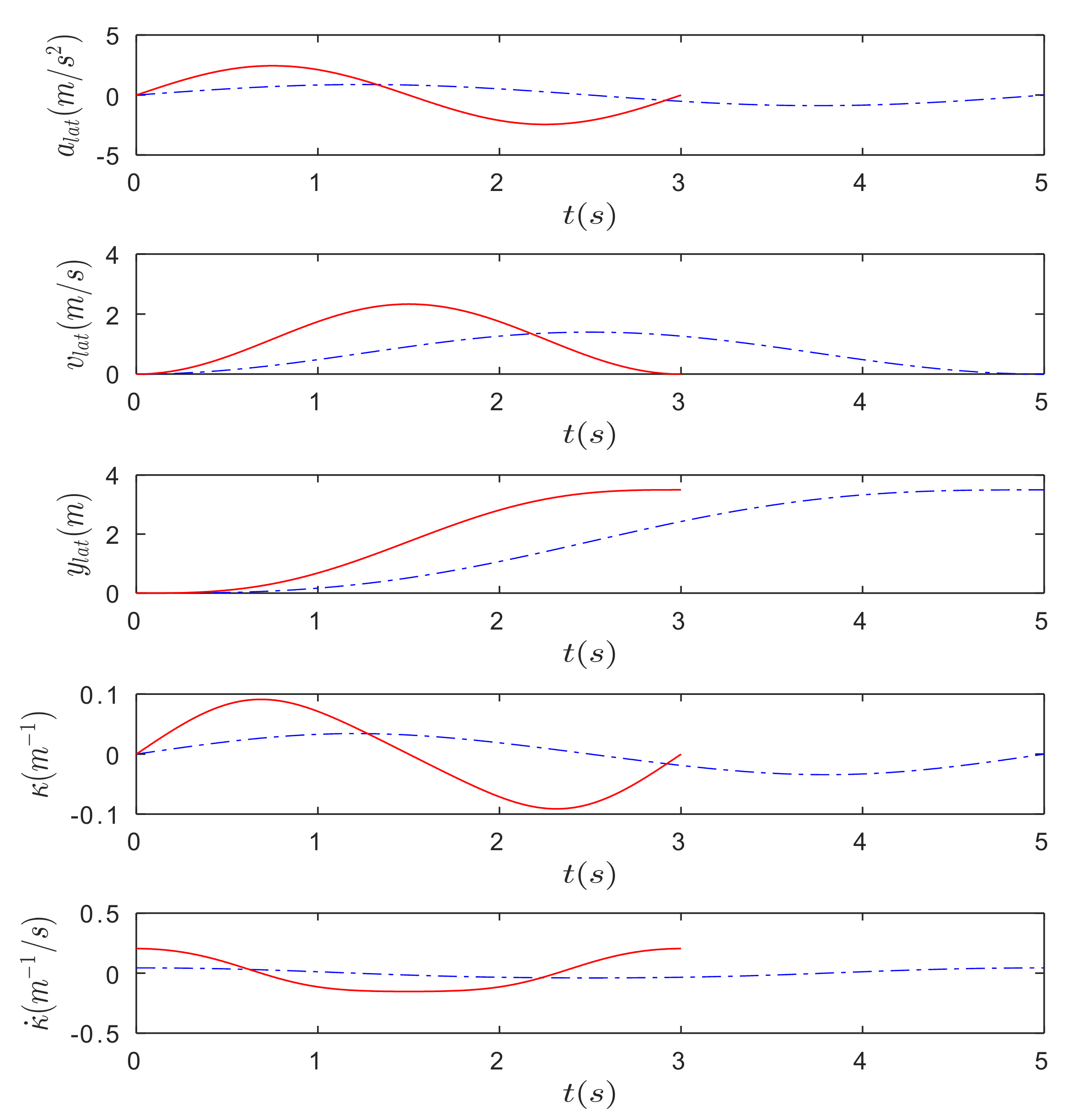
The lateral acceleration, curvature, and lateral velocity of the motion model are differentiable. Assuming that H is 3.5 m, the values of lateral acceleration ${\mathit{a}}_{\mathit{l}\mathit{a}\mathit{t}}$, lateral velocity ${\mathit{v}}_{\mathit{l}\mathit{a}\mathit{t}}$, lateral position ${\mathit{y}}_{\mathit{l}\mathit{a}\mathit{t}}$, curvature k, and derivative of curvature k can be obtained, as shown in Figure 1.

Given the maximum lateral accelerations ${\mathit{a}}_{max,\mathit{l}\mathit{a}\mathit{t}}$ and the total lateral movement distance H, the required time ${\mathit{t}}_{\mathit{l}\mathit{a}\mathit{t}}$ to finish the evasive maneuver can be obtained.

$${\mathit{t}}_{\mathit{l}\mathit{a}\mathit{t}}=\sqrt{2\pi \mathit{H}/{\mathit{a}}_{max,\mathit{l}\mathit{a}\mathit{t}}}$$

(4)

According to natural driving data, the longitudinal and lateral accelerations of the human driver are typically smaller than physically feasible accelerations. For most drivers, the maximum longitudinal and lateral acceleration is around 3~4 ${\mathrm{m}/\mathrm{s}}^2$ at low speed, and can be reduced to 1~2 ${\mathrm{m}/\mathrm{s}}^2$ at high speed [34]. The heading angle in the reference frame can be obtained using longitudinal velocity and lateral velocity.

$$\phi \left(\mathit{t}\right)=\mathit{a}\mathit{r}\mathit{c}\mathit{t}\mathit{a}\mathit{n}({\mathit{v}}_{\mathit{l}\mathit{a}\mathit{t}}\left(\mathit{t}\right)/{\mathit{v}}_{\mathit{l}\mathit{o}\mathit{n}}\left(\mathit{t}\right))$$

(5)

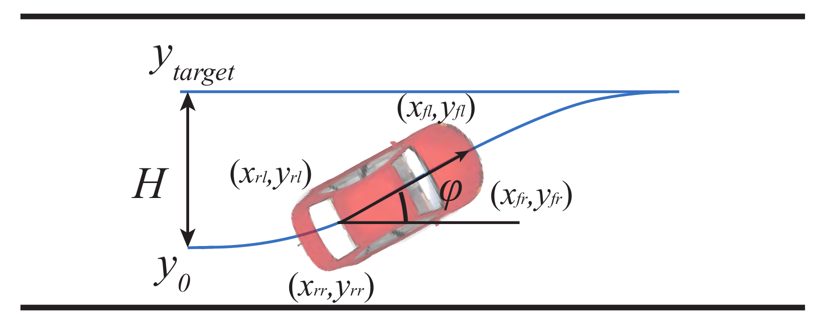
The position of the center of the rear axis can be calculated by the evasive motion model. Thus, the position of each vertex as shown in Figure 2 can be obtained.

$$\begin{array}{cc}\hfill ({\mathit{x}}_{\mathit{f}\mathit{l}},{\mathit{y}}_{\mathit{f}\mathit{l}})=& (\mathit{x}-{\mathit{w}}_{\mathit{h}}\mathit{s}\mathit{i}\mathit{n}\phi +{\mathit{l}}_{\mathit{a}}\mathit{c}\mathit{o}\mathit{s}\phi ,{\mathit{y}}_{\mathit{l}\mathit{a}\mathit{t}}+{\mathit{w}}_{\mathit{h}}\mathit{c}\mathit{o}\mathit{s}\phi +{\mathit{l}}_{\mathit{a}}\mathit{s}\mathit{i}\mathit{n}\phi );\hfill \end{array}$$

(6a)

$$\begin{array}{cc}\hfill ({\mathit{x}}_{\mathit{f}\mathit{r}},{\mathit{y}}_{\mathit{f}\mathit{r}})=& (\mathit{x}+{\mathit{w}}_{\mathit{h}}\mathit{s}\mathit{i}\mathit{n}\phi +{\mathit{l}}_{\mathit{a}}\mathit{c}\mathit{o}\mathit{s}\phi ,{\mathit{y}}_{\mathit{l}\mathit{a}\mathit{t}}-{\mathit{w}}_{\mathit{h}}\mathit{c}\mathit{o}\mathit{s}\phi +{\mathit{l}}_{\mathit{a}}\mathit{s}\mathit{i}\mathit{n}\phi );\hfill \end{array}$$

(6b)

$$\begin{array}{cc}\hfill ({\mathit{x}}_{\mathit{r}\mathit{l}},{\mathit{y}}_{\mathit{r}\mathit{l}})=& (\mathit{x}-{\mathit{w}}_{\mathit{h}}\mathit{s}\mathit{i}\mathit{n}\phi -{\mathit{l}}_{\mathit{b}}\mathit{c}\mathit{o}\mathit{s}\phi ,{\mathit{y}}_{\mathit{l}\mathit{a}\mathit{t}}+{\mathit{w}}_{\mathit{h}}\mathit{c}\mathit{o}\mathit{s}\phi -{\mathit{l}}_{\mathit{b}}\mathit{s}\mathit{i}\mathit{n}\phi );\hfill \end{array}$$

(6c)

$$\begin{array}{cc}\hfill ({\mathit{x}}_{\mathit{r}\mathit{r}},{\mathit{y}}_{\mathit{r}\mathit{r}})=& (\mathit{x}+{\mathit{w}}_{\mathit{h}}\mathit{s}\mathit{i}\mathit{n}\phi -{\mathit{l}}_{\mathit{b}}\mathit{c}\mathit{o}\mathit{s}\phi ,{\mathit{y}}_{\mathit{l}\mathit{a}\mathit{t}}-{\mathit{w}}_{\mathit{h}}\mathit{c}\mathit{o}\mathit{s}\phi -{\mathit{l}}_{\mathit{b}}\mathit{s}\mathit{i}\mathit{n}\phi );\hfill \end{array}$$

(6d)

where, ${\mathit{w}}_{\mathit{h}}$ is the half width of the host vehicle, ${\mathit{l}}_{\mathit{a}}$ and ${\mathit{l}}_{\mathit{b}}$ are the distances from the rear axis to the front most and rear most of the vehicle. $({\mathit{x}}_{\mathit{f}\mathit{l}},{\mathit{y}}_{\mathit{f}\mathit{l}})$ represents the front-left vertex, $({\mathit{x}}_{\mathit{f}\mathit{r}},{\mathit{y}}_{\mathit{f}\mathit{r}})$ represents the front-right vertex, $({\mathit{x}}_{\mathit{r}\mathit{l}},{\mathit{y}}_{\mathit{r}\mathit{l}})$ represents the rear-left vertex, and $({\mathit{x}}_{\mathit{r}\mathit{r}},{\mathit{y}}_{\mathit{r}\mathit{r}})$ represents the rear-right vertex.

As shown in Figure 2, the vehicle moves laterally from ${\mathit{y}}_0$ to ${\mathit{y}}_{\mathit{t}\mathit{a}\mathit{r}\mathit{g}\mathit{e}\mathit{t}}$, the total lateral motion distance is H. At time ${\mathit{t}}_{\phi }$, the heading angle in the reference frame is $\phi$. If a starting lateral position ${\mathit{y}}_0$ and a target lateral position ${\mathit{y}}_{\mathit{t}\mathit{a}\mathit{r}\mathit{g}\mathit{e}\mathit{t}}$ in the reference frame is determined, the time ${\mathit{t}}_{\phi }$ can be obtained based on the motion model.

$$\begin{array}{c}\hfill {\mathit{t}}_{\phi }=\frac{{\mathit{t}}_{\mathit{l}\mathit{a}\mathit{t}}}{2\pi }·\arg cos\left(-\frac{{\mathit{t}}_{\mathit{l}\mathit{a}\mathit{t}}}{\mathit{H}}\left(vtan\phi -\frac{\mathit{H}}{{\mathit{t}}_{\mathit{l}\mathit{a}\mathit{t}}}\right)\right)\end{array}$$

(7)

2.3. The Constraint of Collision Avoidance with Obstacle

The vehicle should avoid collision with static and dynamic obstacles. In this paper, the safe distances for the cases of the lane-keep maneuver, the evasive maneuver, the lane-change maneuver and the lane-change abortion maneuver are studied. For the lateral motion, the evasive motion model in Section 2.2 is utilized.

2.3.1. The Case of Lane-Keep Maneuver

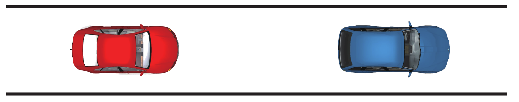
In this paper, the notion of Responsibility-Sensitive Safety (RSS) model [35] for lane-keep maneuver is utilized. If the driver is driving in the lane-keep mode and has no lane-change intention, the safe distances can be obtained for the vehicle following scenario, as shown in Figure 3.

Assuming that the longitudinal velocities of the leading vehicle and the following vehicle at ${\mathit{t}}_0$ are ${\mathit{v}}_{\mathit{f}}$ and ${\mathit{v}}_{\mathit{r}}$. The leading vehicle brakes at acceleration ${\mathit{a}}_{\mathit{f},\mathit{b}\mathit{r}\mathit{a}\mathit{k}\mathit{e}}$. The following vehicle drives with the acceleration ${\mathit{a}}_{\mathit{a}\mathit{c}\mathit{c}\mathit{e}\mathit{l}}$ during the driver’s reaction time ${\mathit{t}}_{\delta }$, then the following vehicle decelerates with the acceleration ${\mathit{a}}_{\mathit{r},\mathit{b}\mathit{r}\mathit{a}\mathit{k}\mathit{e}}$ until stop. During the whole process, the two vehicles should not collide. The safe longitudinal distance between the front-most point of the following vehicle and the rear-most point of the front vehicle at ${\mathit{t}}_0$ is obtained as follows.

$${\mathit{D}}_{\mathrm{safe},\mathrm{follow}}={\mathit{v}}_{\mathit{r}}{\mathit{t}}_{\delta }+\frac{1}{2}{\mathit{a}}_{\mathrm{accel}}{\mathit{t}}_{\delta }^2+\frac{{\left({\mathit{v}}_{\mathit{r}}+{\mathit{a}}_{\mathrm{accel}}{\mathit{t}}_{\delta }\right)}^2}{2{\mathit{a}}_{\mathrm{r},\mathrm{brake}}}-\frac{{\mathit{v}}_{\mathit{f}}^2}{2{\mathit{a}}_{\mathrm{f},\mathrm{brake}}}$$

(8)

In addition, to make sure that ${\mathit{D}}_{\mathit{s}\mathit{a}\mathit{f}\mathit{e},\mathit{f}\mathit{o}\mathit{l}\mathit{l}\mathit{o}\mathit{w}}$ is greater than zero, ${\mathit{v}}_{\mathit{f}}$ follows the condition of ${\mathit{v}}_{\mathit{f}}\le \sqrt{{\mathit{v}}_{\mathit{r}}^2+2{\mathit{v}}_{\mathit{r}}{\mathit{t}}_{\delta }{\mathit{a}}_{\mathit{a}\mathit{c}\mathit{c}\mathit{e}\mathit{l}}}$. If a static obstacle is in front of the host vehicle, we can obtain the safe distance by setting the speed ${\mathit{v}}_{\mathit{f}}$ as zero.

2.3.2. The Case of Evasive Maneuver for Static Obstacle

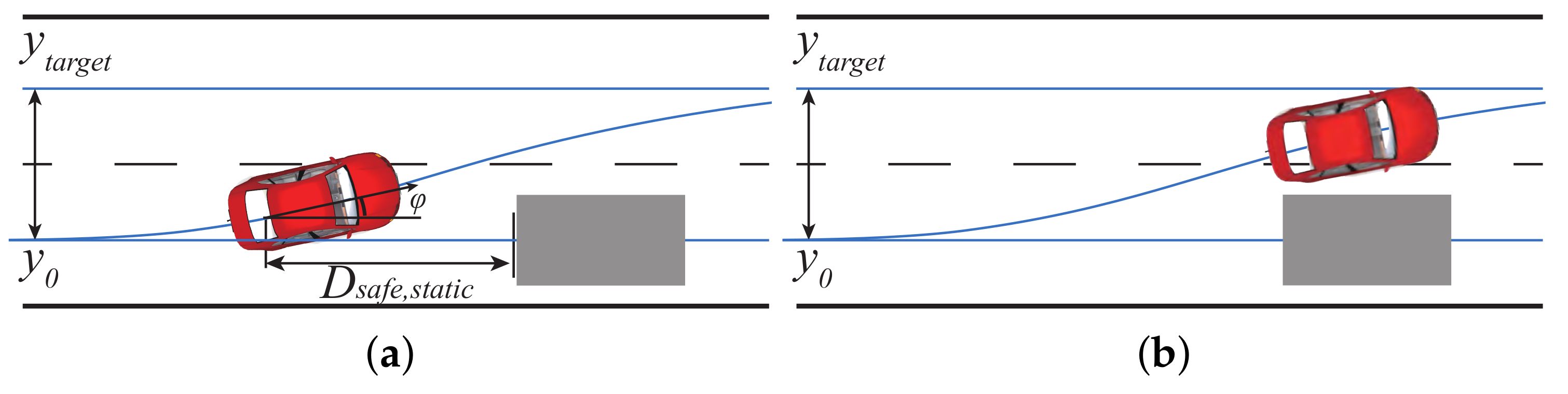
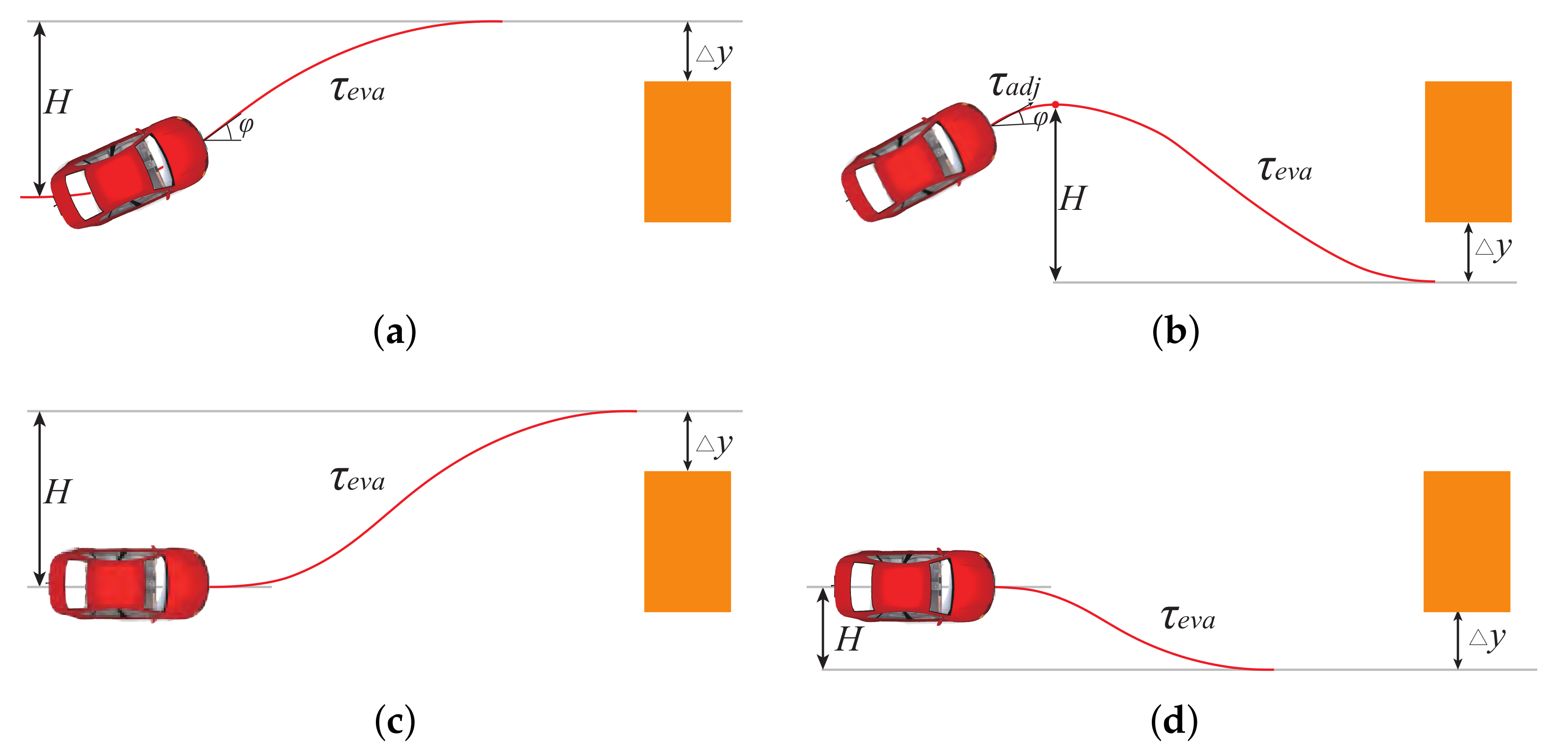
Assuming that there exists a static obstacle in front of the host vehicle, as shown in Figure 4. The heading angle in the reference frame is $\phi$, the lateral position is $\mathit{y}\left({\mathit{t}}_0\right)$, the chosen target lateral position is ${\mathit{y}}_{\mathit{t}\mathit{a}\mathit{r}\mathit{g}\mathit{e}\mathit{t}}$. There are three main steps for calculating the minimum longitudinal safe distance ${\mathit{D}}_{\mathit{s}\mathit{a}\mathit{f}\mathit{e},\mathit{s}\mathit{t}\mathit{a}\mathit{t}\mathit{i}\mathit{c}}$ for avoiding the front static obstacle.

Step I, given the longitudinal acceleration, the current and target lateral position in reference frame, the ${\mathit{t}}_{\phi }$ and ${\mathit{y}}_0$ for lateral motion are obtained according to the evasive motion model described in Section 2.2. By sampling the starting lateral position ${\mathit{y}}_0$ of the evasive motion model, the ${\mathit{t}}_{\phi }$ for each ${\mathit{y}}_0$ can be obtained using Equation (7). By comparing $\mathit{y}\left({\mathit{t}}_{\phi }\right)$ (Equation (2c)) with the current lateral position $\mathit{y}\left({\mathit{t}}_0\right)$, the final ${\mathit{y}}_0$ is determined when $|\mathit{y}\left({\mathit{t}}_0\right)-\mathit{y}\left({\mathit{t}}_{\phi }\right)|$ is less than an error threshold.

Step II, the time ${\mathit{t}}_{\mathit{c}}$ that the vehicle moves from current lateral position (Figure 4a) to the critical lateral position (Figure 4b) is obtained. Assuming the host vehicle follows the evasive motion model, the critical position is defined as the lateral position when the rear-right vertex of the host vehicle just contacts the rear vertex of the convex bounding box of the static obstacle.

Step III, given the longitudinal acceleration a, the longitudinal safe distance for the current lateral position is calculated. Since the time for lateral motion is equal to the time for longitudinal motion, the longitudinal safe distance can be obtained based on the time ${\mathit{t}}_{\mathit{c}}$ of lateral motion.

$${\mathit{D}}_{\mathit{s}\mathit{a}\mathit{f}\mathit{e},\mathit{s}\mathit{t}\mathit{a}\mathit{t}\mathit{i}\mathit{c}}={\mathit{v}}_{\mathit{M}}\left(0\right){\mathit{t}}_{\mathit{c}}+\frac{1}{2}\mathit{a}{\mathit{t}}_{\mathit{c}}^2+\epsilon$$

(9)

where ${\mathit{v}}_{\mathit{M}}\left(0\right)$ is the current speed of the host vehicle, $\epsilon$ is a constant that compensates for the distance error of the motion model.

2.3.3. The Case of Lane-Change Maneuver

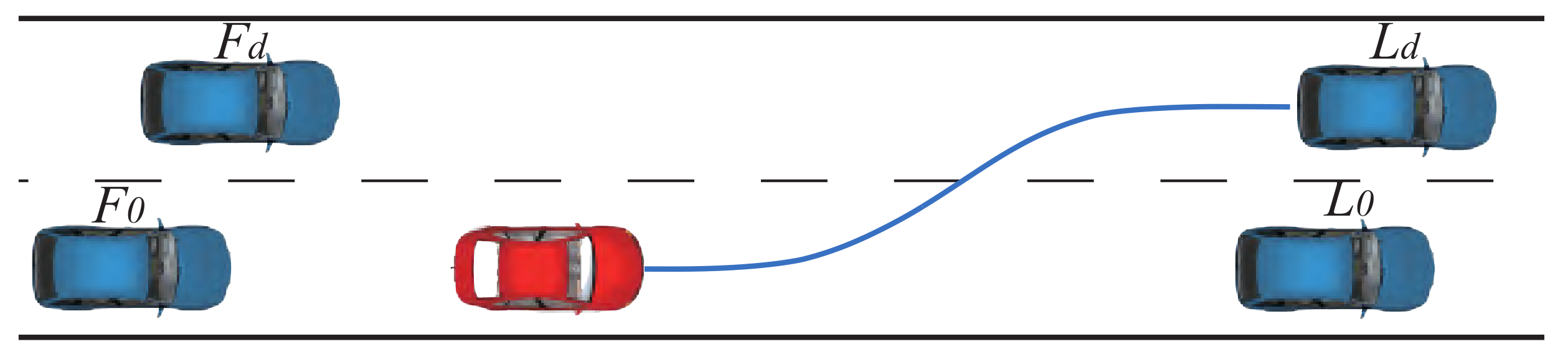
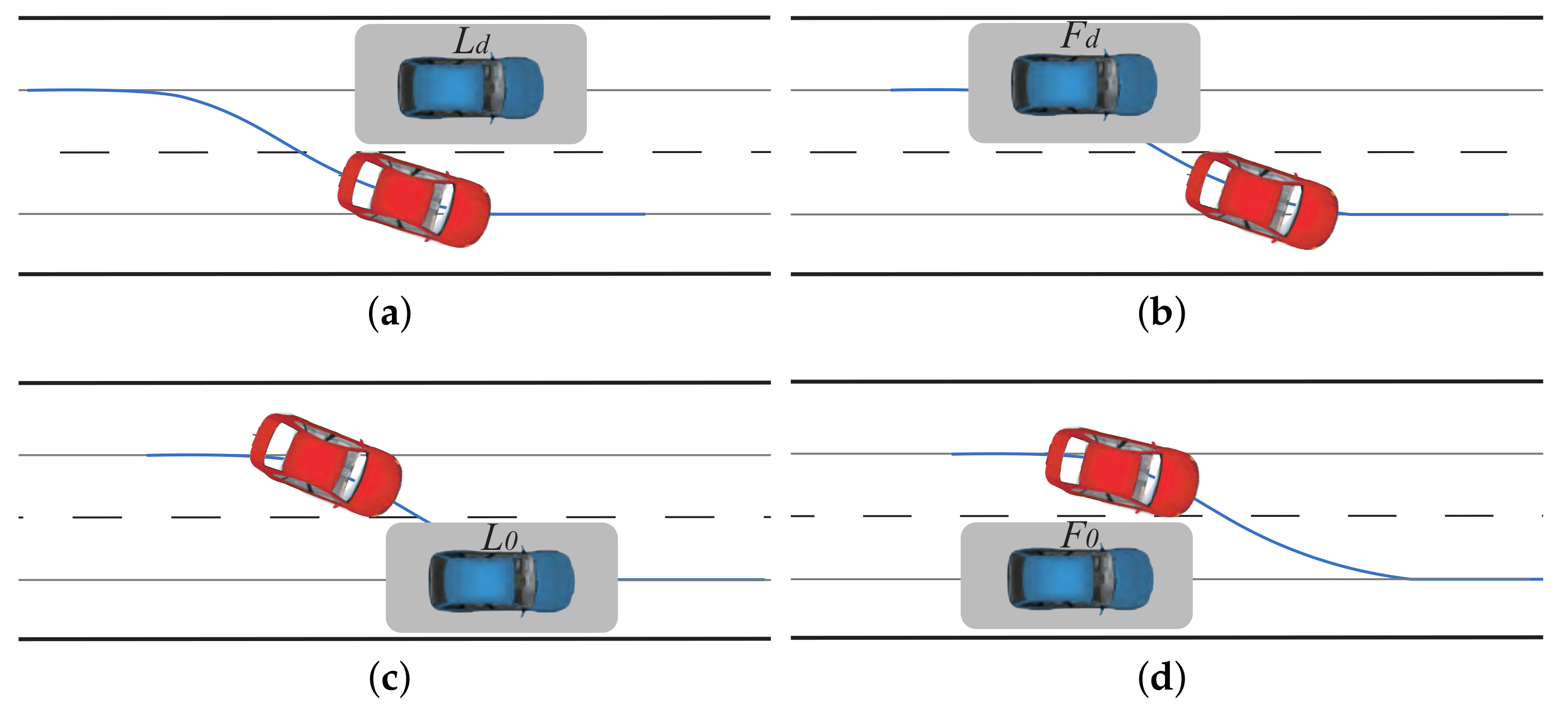
In [9], the longitudinal safe distance to start a lane-change maneuver is derived. However, the longitudinal safe distance during a lane change maneuver is not derived. Inspired by [9], the safe distance during the lane-change process and the lane-change abortion process have been discussed in our previous work [36]. In this paper, the prediction uncertainty is considered to obtain the safe distance for lane change. A lane-change scenario is shown in Figure 5, the front vehicle ${\mathit{L}}_0$ and rear vehicle ${\mathit{F}}_0$ are in the current lane, the front vehicle ${\mathit{L}}_{\mathit{d}}$ and the rear vehicle ${\mathit{F}}_{\mathit{d}}$ are in the left target lane.

If considering the uncertainty of prediction, the occupancy area of traffic participants at each prediction step can be obtained. The constant acceleration lane keeping (CALK) model [37] can be used to represent the motion of lane-keep considering uncertainty.

$${\left[\begin{array}{c}\mathit{s}\\ \mathit{n}\\ {\mathit{v}}_{\mathit{s}}\\ {\mathit{a}}_{\mathit{s}}\end{array}\right]}_{\mathit{k}}=\left[\begin{array}{cccc}1& 0& \Delta \mathit{t}& \frac{\Delta {\mathit{t}}^2}{2}\\ 0& 1& 0& 0\\ 0& 0& 1& \Delta \mathit{t}\\ 0& 0& 0& 1\end{array}\right]{\left[\begin{array}{c}\mathit{s}\\ \mathit{n}\\ {\mathit{v}}_{\mathit{s}}\\ {\mathit{a}}_{\mathit{s}}\end{array}\right]}_{\mathit{k}-1}+\left[\begin{array}{c}{\mathit{w}}_{\mathit{a}\mathit{s}}\Delta {\mathit{t}}^2/2\\ {\mathit{w}}_{\mathit{a}\mathit{n}}\Delta {\mathit{t}}^2/2\\ {\mathit{w}}_{\mathit{a}\mathit{s}}\Delta \mathit{t}\\ {\mathit{w}}_{\mathit{a}\mathit{s}}\end{array}\right]$$

(10)

where ${\mathit{w}}_{\mathit{a}\mathit{s}}\sim \mathit{N}(0,{\sigma }_{\mathit{a}\mathit{s}}^2)$, ${\mathit{w}}_{\mathit{a}\mathit{n}}\sim \mathit{N}(0,{\sigma }_{\mathit{a}\mathit{n}}^2)$. Since the vehicle is in lane keeping mode, the lateral position is bounded in the lane.

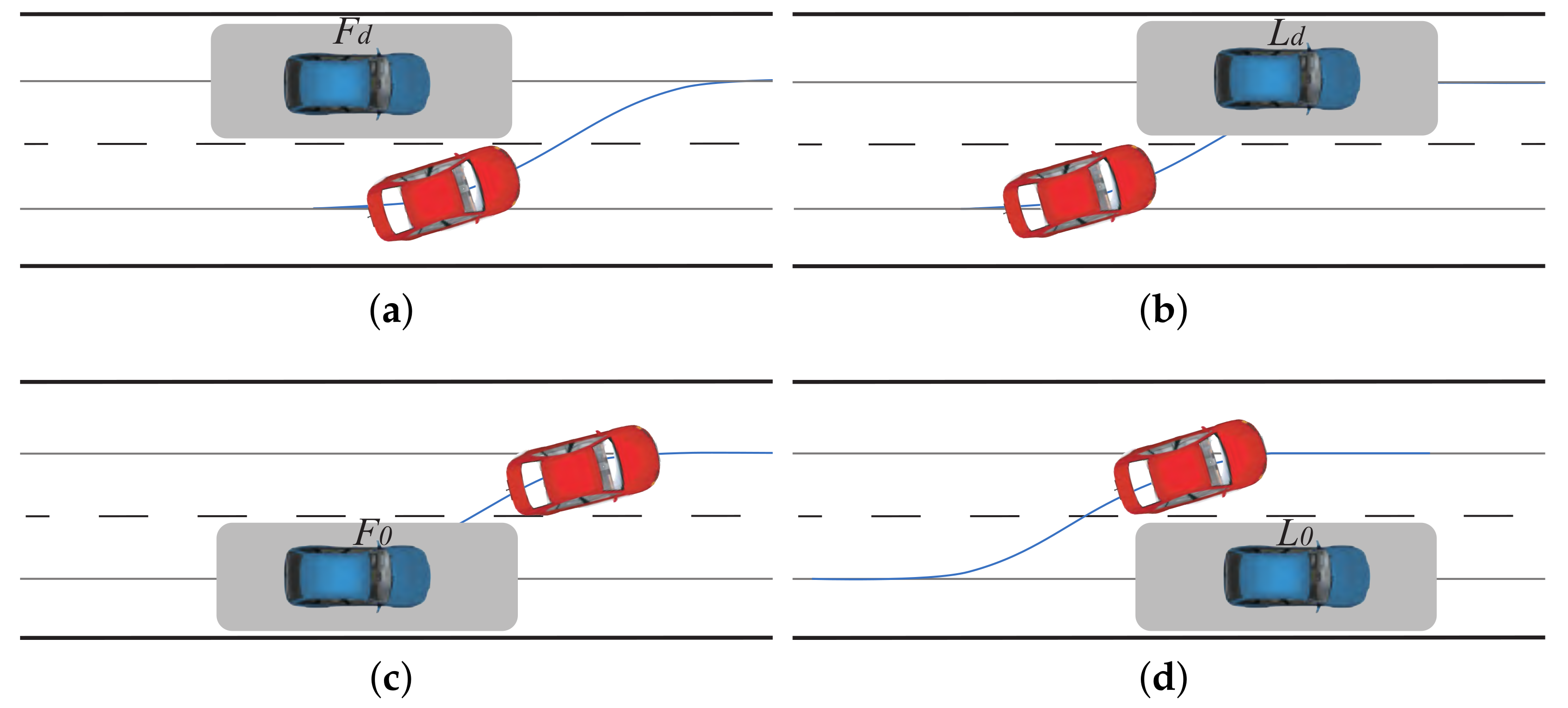
The critical situation for calculating the longitudinal safe distance considering uncertainty is defined as Figure 6. The vertex of the host vehicle just touches the vertex of the occupancy set of the traffic participant.

The time it takes for the host vehicle to move from the current lateral position to the lateral position defined in Figure 6 can be obtained according to Section 2.2. First of all, we calculate the time to arrive at the lateral position defined in Figure 6. Then, the longitudinal safe distance for each vehicle is obtained based on the time to arrive at the critical time. The minimum longitudinal safe distance ${\mathit{D}}_{\mathit{F}\mathit{d},\mathit{s}}$, ${\mathit{D}}_{\mathit{L}\mathit{d},\mathit{s}}$, ${\mathit{D}}_{\mathit{F}0,\mathit{s}}$, ${\mathit{D}}_{\mathit{L}0,\mathit{s}}$ for vehicles ${\mathit{F}}_{\mathit{d}}$, ${\mathit{L}}_{\mathit{d}}$, ${\mathit{F}}_0$, ${\mathit{L}}_0$ during the process of the lane-change maneuver can be derived as Equation (11).

$$\begin{array}{cc}\hfill {\mathit{D}}_{\mathit{F}\mathit{d},\mathit{s}}=& \underset{\mathit{t}}{\mathit{m}\mathit{a}\mathit{x}}\left({\int }_0^{\mathit{t}}{\int }_0^{\lambda }\left({\mathit{a}}_{\mathit{F}\mathit{d}}\left(\tau \right)-{\mathit{a}}_{\mathit{M}}\left(\tau \right)\right)\mathit{d}\tau \mathit{d}\lambda +\left({\mathit{v}}_{\mathit{F}\mathit{d}}\left(0\right)-{\mathit{v}}_{\mathit{M}}\left(0\right)\right)\mathit{t}\right),\forall \mathit{t}\in \left[{\mathit{t}}_{\mathit{c},\mathit{F}\mathit{d}},\mathit{T}\right]\hfill \end{array}$$

(11a)

$$\begin{array}{cc}\hfill {\mathit{D}}_{\mathit{L}\mathit{d},\mathit{s}}=& \underset{\mathit{t}}{\mathit{m}\mathit{a}\mathit{x}}\left({\int }_0^{\mathit{t}}{\int }_0^{\lambda }\left({\mathit{a}}_{\mathit{M}}\left(\tau \right)-{\mathit{a}}_{\mathit{L}\mathit{d}}\left(\tau \right)\right)\mathit{d}\tau \mathit{d}\lambda +\left({\mathit{v}}_{\mathit{M}}\left(0\right)-{\mathit{v}}_{\mathit{L}\mathit{d}}\left(0\right)\right)\mathit{t}\right),\forall \mathit{t}\in \left[{\mathit{t}}_{\mathit{c},\mathit{L}\mathit{d}},\mathit{T}\right]\hfill \end{array}$$

(11b)

$$\begin{array}{cc}\hfill {\mathit{D}}_{\mathit{F}0,\mathit{s}}=& \underset{\mathit{t}}{\mathit{m}\mathit{a}\mathit{x}}\left\{\left({\int }_0^{\mathit{t}}{\int }_0^{\lambda }\left({\mathit{a}}_{{\mathit{F}}_0}\left(\tau \right)-{\mathit{a}}_{\mathit{M}}\left(\tau \right)\right)\mathit{d}\tau \mathit{d}\lambda +\left({\mathit{v}}_{{\mathit{F}}_0}\left(0\right)-{\mathit{v}}_{\mathit{M}}\left(0\right)\right)\mathit{t}\right),0\right\},\forall \mathit{t}\in \left[0,{\mathit{t}}_{\mathit{c},\mathit{F}0}\right]\hfill \end{array}$$

(11c)

$$\begin{array}{cc}\hfill {\mathit{D}}_{\mathit{L}0,\mathit{s}}=& \underset{\mathit{t}}{\mathit{m}\mathit{a}\mathit{x}}\left\{\left({\int }_0^{\mathit{t}}{\int }_0^{\lambda }\left({\mathit{a}}_{\mathit{M}}\left(\tau \right)-{\mathit{a}}_{\mathit{L}\mathit{o}}\left(\tau \right)\right)\mathit{d}\tau \mathit{d}\lambda +\left({\mathit{v}}_{\mathit{M}}\left(0\right)-{\mathit{v}}_{\mathit{L}\mathit{o}}\left(0\right)\right)\mathit{t}\right),0\right\}\forall \mathit{t}\in \left[0,{\mathit{t}}_{\mathit{c},\mathit{L}0}\right]\hfill \end{array}$$

(11d)

where ${\mathit{t}}_{\mathit{c},\mathit{F}\mathit{d}}$, ${\mathit{t}}_{\mathit{c},\mathit{L}\mathit{d}}$, ${\mathit{t}}_{\mathit{c},\mathit{F}0}$, ${\mathit{t}}_{\mathit{c},\mathit{L}0}$ are the time it takes for the host vehicle to move from current state to the defined critical lateral position in Figure 6. ${\mathit{a}}_{\mathit{M}}$ is the acceleration of the host vehicle, ${\mathit{a}}_{\mathit{F}\mathit{d}}$, ${\mathit{a}}_{\mathit{L}\mathit{d}}$, ${\mathit{a}}_{\mathit{F}0}$, ${\mathit{a}}_{\mathit{L}0}$ are the accelerations of the vehicles ${\mathit{F}}_{\mathit{d}}$, ${\mathit{L}}_{\mathit{d}}$, ${\mathit{F}}_0$, ${\mathit{L}}_0$. By Substituting the motion model in Equation (10) into Equation (11), the minimum safe distances during the lane change process considering prediction uncertainty are obtained.

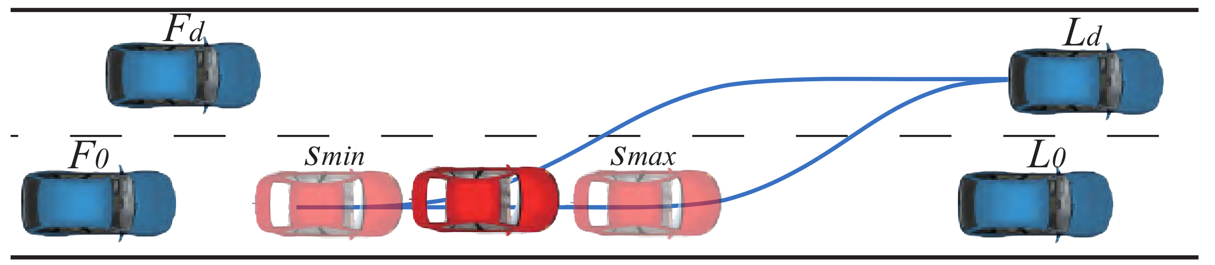
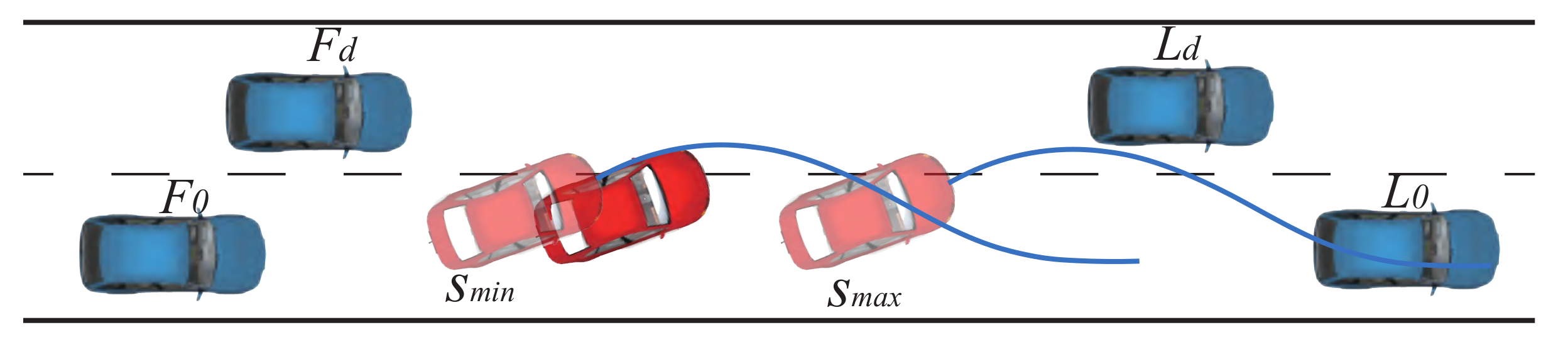
If the host vehicle is preparing for lane-change or is under the lane-change process, ${\mathit{s}}_{\mathit{m}\mathit{i}\mathit{n}}$ is the minimum safe longitudinal position, ${\mathit{s}}_{\mathit{m}\mathit{a}\mathit{x}}$ is the maximum safe longitudinal position, shown as the shadowed red vehicles in Figure 7. The safe longitudinal position s should satisfy the constraint ${\mathit{s}}_{\mathit{m}\mathit{i}\mathit{n}}\le \mathit{s}\le {\mathit{s}}_{\mathit{m}\mathit{a}\mathit{x}}$. If the host vehicle starts lateral motion at ${\mathit{s}}_{\mathit{m}\mathit{a}\mathit{x}}$, it will arrive at the critical position with the front vehicle ${\mathit{L}}_0$ or the front vehicle ${\mathit{L}}_{\mathit{d}}$, as shown in Figure 6b,d. If the host vehicle starts lateral motion at ${\mathit{s}}_{\mathit{m}\mathit{i}\mathit{n}}$, it will arrive at the critical position with the rear vehicle ${\mathit{F}}_0$ or the rear vehicle ${\mathit{F}}_{\mathit{d}}$, as shown in Figure 6a,b. The safe longitudinal position of the host vehicle should be in $[{\mathit{x}}_{\mathit{m}\mathit{i}\mathit{n},\mathit{s}\mathit{a}\mathit{f}\mathit{e}},{\mathit{x}}_{\mathit{m}\mathit{a}\mathit{x},\mathit{s}\mathit{a}\mathit{f}\mathit{e}}]$.

$$\begin{array}{c}\hfill {\mathit{x}}_{\mathit{m}\mathit{i}\mathit{n},\mathit{s}\mathit{a}\mathit{f}\mathit{e}}=\mathit{m}\mathit{a}\mathit{x}({\mathit{s}}_{\mathit{F}0}+{\mathit{D}}_{\mathit{F}0,\mathit{s}},{\mathit{s}}_{\mathit{F}\mathit{d}}+{\mathit{D}}_{\mathit{F}\mathit{d},\mathit{s}})\\ \hfill {\mathit{x}}_{\mathit{m}\mathit{a}\mathit{x},\mathit{s}\mathit{a}\mathit{f}\mathit{e}}=\mathit{m}\mathit{i}\mathit{n}({\mathit{s}}_{\mathit{L}0}-{\mathit{D}}_{\mathit{L}0,\mathit{s}},{\mathit{s}}_{\mathit{L}\mathit{d}}-{\mathit{D}}_{\mathit{L}\mathit{d},\mathit{s}})\end{array}$$

where ${\mathit{s}}_{\mathit{F}\mathit{d}}$, ${\mathit{s}}_{\mathit{F}0}$, ${\mathit{s}}_{\mathit{L}\mathit{d}}$, ${\mathit{s}}_{\mathit{L}0}$ are the longitudinal positions of the vehicles ${\mathit{F}}_{\mathit{d}}$, ${\mathit{F}}_0$, ${\mathit{L}}_{\mathit{d}}$, ${\mathit{L}}_0$; ${\mathit{D}}_{\mathit{L}\mathit{d},\mathit{s}}$, ${\mathit{D}}_{\mathit{L}0,\mathit{s}}$, ${\mathit{D}}_{\mathit{F}\mathit{d},\mathit{s}}$, ${\mathit{D}}_{\mathit{F}0,\mathit{s}}$ are the required minimum safe longitudinal distances for the surrounding vehicles for a lane-change maneuver.

2.3.4. The Case of Lane-Change Abortion

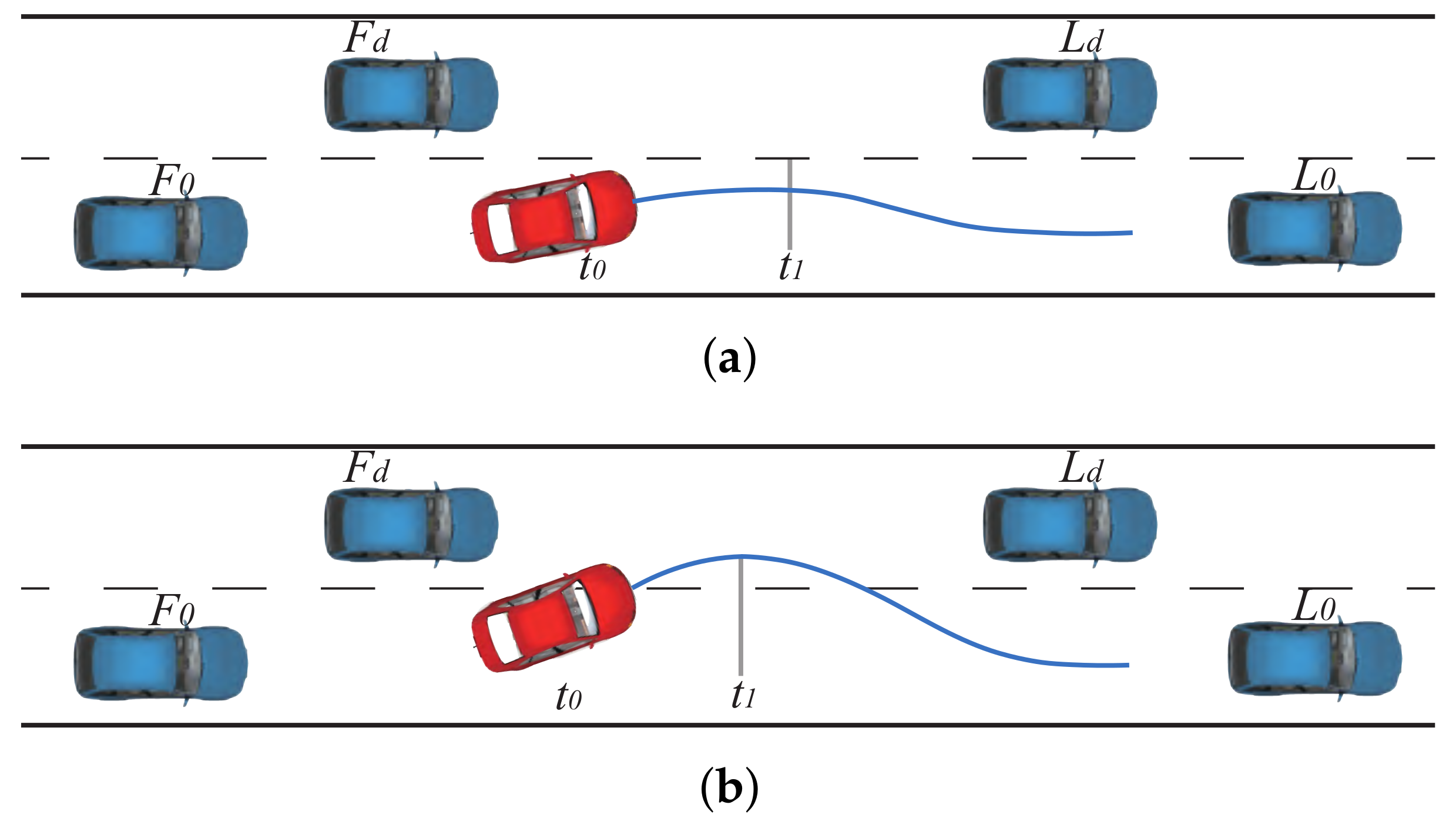
During the lane change process, if the other vehicles take non-cooperative driving behavior, the condition for lane-change may no longer be satisfied due to the insufficient gap. The driving assistant system should evaluate whether the host vehicle can safely cancel the lane-change maneuver. For a lane-change abortion maneuver, there are two cases as shown in Figure 8. In the first case, the host vehicle cancels lane-change maneuver in a lane-keep mode if it will not enter the left target lane, as shown in Figure 8a. Only the front vehicle ${\mathit{L}}_0$ and the rear vehicle ${\mathit{F}}_0$ should be considered in the first case. In the second case, the host vehicle cancels lane-change maneuver in a lane-change mode if it will enter the target lane, as shown in Figure 8b. The surrounding vehicles in both lanes should be considered in the second case. During time $[{\mathit{t}}_0,{\mathit{t}}_1]$, the vehicle adjusts the lateral velocity until the lateral velocity equals to zero at ${\mathit{t}}_1$ . The two cases can be classified according to the lateral position $\mathit{y}\left({\mathit{t}}_1\right)$ at time ${\mathit{t}}_1$. Assuming that the host vehicle moves at a constant lateral acceleration ${\mathit{a}}_{\mathit{l}\mathit{a}\mathit{t},\mathit{a}\mathit{d}\mathit{j}}$ during time $[{\mathit{t}}_0,{\mathit{t}}_1]$. The time ${\mathit{t}}_1$ can be obtained ${\mathit{t}}_1={\mathit{v}}_{\mathit{l}\mathit{a}\mathit{t}}/{\mathit{a}}_{\mathit{l}\mathit{a}\mathit{t},\mathit{a}\mathit{d}\mathit{j}}$. We can have the lateral position $\mathit{y}\left({\mathit{t}}_1\right)$ at time ${\mathit{t}}_1$.

$$\mathit{y}\left({\mathit{t}}_1\right)={\mathit{y}}_0+{\mathit{v}}_{\mathit{l}\mathit{a}\mathit{t}}{\mathit{t}}_1-\frac{1}{2}{\mathit{a}}_{\mathit{l}\mathit{a}\mathit{t}}{\mathit{t}}_1^2$$

(12)

In the second case, at time ${\mathit{t}}_1$, the left lane-change abortion scenario in Figure 8b is the same as a right lane-change scenario. Considering the uncertainty of prediction, the defined critical lateral position for a right lane-change maneuver is shown in Figure 9.

The minimum longitudinal safe distances for lane-change abortion are as follows.

$$\begin{array}{cc}\hfill {\mathit{D}}_{\mathit{L}\mathit{d},\mathit{s}}=& \underset{\mathit{t}}{max}\left({\int }_0^{\mathit{t}}{\int }_0^{\lambda }\left({\mathit{a}}_{\mathit{m}}\left(\tau \right)-{\mathit{a}}_{\mathit{L}\mathit{d}}\left(\tau \right)\right)\mathit{d}\tau \mathit{d}\lambda +\left({\mathit{v}}_{\mathit{m}}-{\mathit{v}}_{\mathit{L}\mathit{d}}\right)\mathit{t}\right),\forall \mathit{t}\in \left[0,{\mathit{t}}_1+{\mathit{t}}_{\mathit{c},\mathit{L}\mathit{d}}\right]\hfill \end{array}$$

(13a)

$$\begin{array}{cc}\hfill {\mathit{D}}_{\mathit{F}\mathit{d},\mathit{s}}=& \underset{\mathit{t}}{max}\left({\int }_0^{\mathit{t}}{\int }_0^{\lambda }\left({\mathit{a}}_{\mathit{F}\mathit{d}}\left(\tau \right)-{\mathit{a}}_{\mathit{m}}\left(\tau \right)\right)\mathit{d}\tau \mathit{d}\lambda +\left({\mathit{v}}_{\mathit{F}\mathit{d}}-{\mathit{v}}_{\mathit{m}}\right)\mathit{t}\right),\forall \mathit{t}\in \left[0,{\mathit{t}}_1+{\mathit{t}}_{\mathit{c},\mathit{F}\mathit{d}}\right]\hfill \end{array}$$

(13b)

$$\begin{array}{cc}\hfill {\mathit{D}}_{\mathit{L}0,\mathit{s}}=& \underset{\mathit{t}}{max}\left({\int }_0^{\mathit{t}}{\int }_0^{\lambda }\left({\mathit{a}}_{\mathit{m}}\left(\tau \right)-{\mathit{a}}_{\mathit{L}0}\left(\tau \right)\right)\mathit{d}\tau \mathit{d}\lambda +\left({\mathit{v}}_{\mathit{m}}-{\mathit{v}}_{\mathit{L}0}\right)\mathit{t}\right),\forall \mathit{t}\in \left[{\mathit{t}}_1+{\mathit{t}}_{\mathit{c},\mathit{L}0},\mathit{T}\right]\hfill \end{array}$$

(13c)

$$\begin{array}{cc}\hfill {\mathit{D}}_{\mathit{F}0,\mathit{s}}=& \underset{\mathit{t}}{max}\left({\int }_0^{\mathit{t}}{\int }_0^{\lambda }\left({\mathit{a}}_{\mathit{F}0,\mathit{s}}\left(\tau \right)-{\mathit{a}}_{\mathit{m}}\left(\tau \right)\right)\mathit{d}\tau \mathit{d}\lambda +\left({\mathit{v}}_{\mathit{F}0}-{\mathit{v}}_{\mathit{m}}\right)\mathit{t}\right),\forall \mathit{t}\in \left[{\mathit{t}}_1+{\mathit{t}}_{\mathit{c},\mathit{F}0},\mathit{T}\right]\hfill \end{array}$$

(13d)

where, ${\mathit{t}}_1$ is the time it takes to adjust the lateral velocity to zero, ${\mathit{t}}_{\mathit{c},\mathit{x}}$ is the time it takes to move laterally from the lateral position $\mathit{y}\left({\mathit{t}}_1\right)$ to the lateral position defined in Figure 9. ${\mathit{a}}_{\mathit{L}\mathit{d}}$, ${\mathit{a}}_{\mathit{F}\mathit{d}}$, ${\mathit{a}}_{\mathit{L}0}$, ${\mathit{a}}_{\mathit{F}0}$ are the accelerations of vehicle ${\mathit{L}}_{\mathit{d}}$, ${\mathit{F}}_{\mathit{d}}$, ${\mathit{L}}_0$, ${\mathit{F}}_0$. ${\mathit{v}}_{\mathit{L}\mathit{d}}$, ${\mathit{v}}_{\mathit{F}\mathit{d}}$, ${\mathit{v}}_{\mathit{L}0}$, ${\mathit{v}}_{\mathit{F}0}$ are the speeds of vehicle ${\mathit{L}}_{\mathit{d}}$, ${\mathit{F}}_{\mathit{d}}$, ${\mathit{L}}_0$, ${\mathit{F}}_0$. ${\mathit{v}}_{\mathit{m}}$ and ${\mathit{a}}_{\mathit{m}}$ are the acceleration and speed of the host vehicle. T is the prediction horizon. The minimum and maximum longitudinal position for lane-change abortion maneuver is shown in Figure 10. If the host vehicle cancels lane-change maneuver at ${\mathit{s}}_{\mathit{m}\mathit{i}\mathit{n}}$, it will arrive at the critical position with rear vehicle ${\mathit{F}}_{\mathit{d}}$ or ${\mathit{F}}_0$ (shown in Figure 9b and Figure 9d). If the host vehicle cancels lane-change maneuver at ${\mathit{s}}_{\mathit{m}\mathit{a}\mathit{x}}$, it will arrive at the critical position with front vehicle ${\mathit{L}}_{\mathit{d}}$ or ${\mathit{L}}_0$ (shown in Figure 9a,c).

3. The Driving Envelope for Candidate Driving Maneuvers

We propose a novel driving envelope, which is a collision-free area for the host vehicle. Since the evasive motion model is used, the safe area during the entire phase of a lane-change maneuver can be obtained quickly. The constraints of the vehicle motion, the limit of steering of the driver, and avoiding collision with road boundary and obstacles are considered.

3.1. The Reachable-Set Considering Driver’s Input

The reachable-set is a useful tool for human-in-the-loop systems to determine the boundary of executable trajectories [27]. For a system f, the system dynamic is $\dot{\mathit{x}}\left(\mathit{t}\right)=\mathit{f}(\mathit{x}\left(\mathit{t}\right),\mathit{u}\left(\mathit{t}\right))$ under an allowable control signal u. Given an initial state ${\mathit{x}}_0$, an input signal $\mathit{u}\left(\mathit{t}\right)$, and the system dynamics $\dot{\mathit{x}}\left(\mathit{t}\right)=\mathit{f}\left(\mathit{x}\left(\mathit{t}\right),\mathit{u}\left(\mathit{t}\right)\right)$, the reachable set $\mathcal{R}\left(\mathit{t}\right)$ is defined as the set of all states that can be reached from an initial set ${\mathcal{X}}^0$ at time t.

$$\begin{array}{c}\hfill \mathcal{R}\left(\mathit{t}\right)=\left\{{\mathit{x}}_0+{\int }_0^{\mathit{t}}\mathit{f}\left(\mathit{x}\left(\tau \right),\mathit{u}\left(\tau \right)\right)\mathit{d}\tau |{\mathit{x}}_0\in {\mathcal{X}}^0,\forall \mathit{t}:\mathit{u}\left(\mathit{t}\right)\in \mathcal{U}\right\}\end{array}$$

(14)

Due to the constraint of the machinery steering structure, the curvature of the trajectory should not exceed the maximum boundary ${\kappa }_{\mathit{m}\mathit{e}\mathit{c}\mathit{h},\mathit{m}\mathit{a}\mathit{x}}$. To avoid severe sideslip, the curvature is limited by maximum lateral acceleration ${\mathit{a}}_{\mathit{l}\mathit{a}\mathit{t},\mathit{m}\mathit{a}\mathit{x}}$.

$${\kappa }_{\mathit{m}\mathit{a}\mathit{x}}=min({\kappa }_{\mathit{m}\mathit{e}\mathit{c}\mathit{h},\mathit{m}\mathit{a}\mathit{x}},{\mathit{a}}_{\mathit{l}\mathit{a}\mathit{t},\mathit{m}\mathit{a}\mathit{x}}/{\mathit{v}}^2)$$

(15)

Considering the driving characteristics, the steering maneuver should not be too hasty, and the path curvature should changes smoothly.

$$\kappa \left(\mathit{s}\right)={\kappa }_0+{\mathit{k}}_{\mathit{r}\mathit{a}\mathit{t}\mathit{e}}·\mathit{s}$$

(16)

where ${\mathit{k}}_{\mathit{r}\mathit{a}\mathit{t}\mathit{e}}$ represents the change rate of curvature as the trajectory length increases, ${\kappa }_0$ represents the initial curvature, and it is influenced by the front wheel angle. s represents the arc length of the trajectory.

$${\kappa }_0=tan\delta /\mathit{L}$$

(17)

If the vehicle moves at constant acceleration a, then the length s can be calculated by the uniform acceleration motion formula.

$$\mathit{s}={\mathit{v}}_0\mathit{t}+\frac{1}{2}\mathit{a}{\mathit{t}}^2$$

(18)

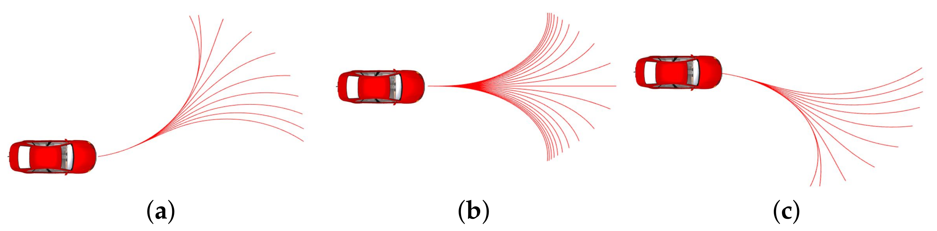
The curvature and the change rate of curvature are limited in a reasonable range, $\kappa \in \left[-{\kappa }_{max},{\kappa }_{max}\right]$, ${\mathit{k}}_{\mathit{r}\mathit{a}\mathit{t}\mathit{e}}\in \left[-{\kappa }_{\mathit{r}\mathit{a}\mathit{t}\mathit{e},\mathit{m}\mathit{a}\mathit{x}},{\kappa }_{\mathit{r}\mathit{a}\mathit{t}\mathit{e},\mathit{m}\mathit{a}\mathit{x}}\right]$. By discretizing the curvature rate ${\mathit{k}}_{\mathit{r}\mathit{a}\mathit{t}\mathit{e}}$, the executable trajectory range of the vehicle in the finite time domain can be obtained, as shown in Figure 11.

$$\begin{array}{cc}\hfill \mathit{x}\left(\mathit{s}\right)& ={\int }_{{\mathit{s}}_0}^{\mathit{s}}cos\left(\theta \left(\tau \right)\right)\mathit{d}\tau +\mathit{x}\left({\mathit{s}}_0\right)\hfill \\ \hfill \mathit{y}\left(\mathit{s}\right)& ={\int }_{{\mathit{s}}_0}^{\mathit{s}}sin\left(\theta \left(\tau \right)\right)\mathit{d}\tau +\mathit{y}\left({\mathit{s}}_0\right)\hfill \\ \hfill \theta \left(\mathit{s}\right)& ={\int }_{{\mathit{s}}_0}^{\mathit{s}}\kappa \left(\tau \right)\mathit{d}\tau +\theta \left({\mathit{s}}_0\right)\hfill \end{array}$$

(19)

3.2. The Driving Envelope with Road Constraint and Steering Limitation

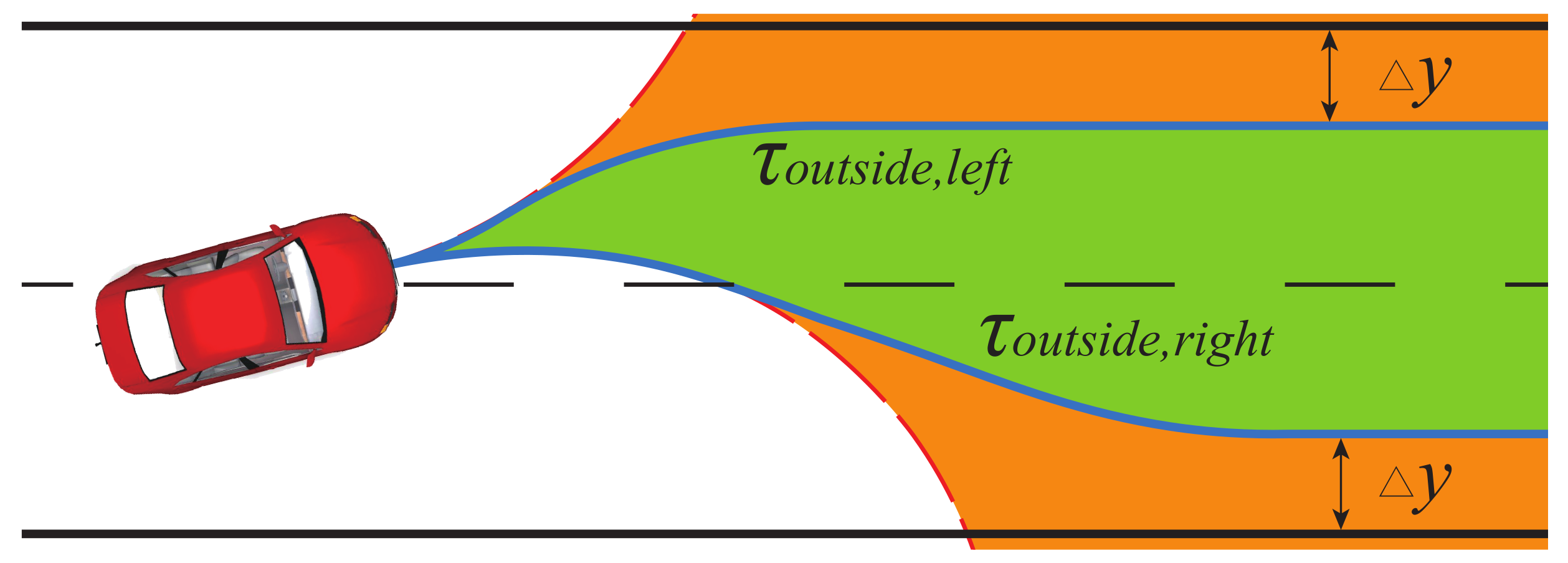
Given the initial state and the maximum curvature rate ${\mathit{k}}_{\mathit{r}\mathit{a}\mathit{t}\mathit{e},\mathit{m}\mathit{a}\mathit{x}}$ of the vehicle, the reachable-set can be obtained shown as the orange area within the dashed lines in Figure 12. This reachable set considers the initial vehicle states, driver’s input, and steering limitation. However, avoiding collision with the lane boundary has not been considered. The evasive motion model can guarantee safe motion avoiding collision with obstacles and lane boundaries. However, the initial steering angle and steering limitation are not considered. We combine the evasive motion model and the boundary of reachable-set to overcome the disadvantages. Considering the road boundary constraint, we set aside a safe distance $\Delta \mathit{y}$ to the road boundary to get the target lateral position. By utilizing the evasive motion model in Section 2.2, a path arriving at the target lateral position can be obtained. We connect the boundary of the reachable-set (Section 3.1) and the path following the evasive motion model to obtain the boundary paths of driving envelope, denoted as ${\tau }_{\mathit{o}\mathit{u}\mathit{t}\mathit{s}\mathit{i}\mathit{d}\mathit{e},\mathit{l}\mathit{e}\mathit{f}\mathit{t}}$ and ${\tau }_{\mathit{o}\mathit{u}\mathit{t}\mathit{s}\mathit{i}\mathit{d}\mathit{e},\mathit{r}\mathit{i}\mathit{g}\mathit{h}\mathit{t}}$ in Figure 12. On the connection point, the curvatures of the two paths are equal, so that the continuity of curvature at the connection point could be guaranteed. The ${\tau }_{\mathit{o}\mathit{u}\mathit{t}\mathit{s}\mathit{i}\mathit{d}\mathit{e},\mathit{l}\mathit{e}\mathit{f}\mathit{t}}$ and ${\tau }_{\mathit{o}\mathit{u}\mathit{t}\mathit{s}\mathit{i}\mathit{d}\mathit{e},\mathit{r}\mathit{i}\mathit{g}\mathit{h}\mathit{t}}$ can be treated as the boundary path of driving envelope considering the constraints of lane boundary and steering limitation. The green area ${\mathit{R}}_{\mathit{s}}$ between ${\tau }_{\mathit{o}\mathit{u}\mathit{t}\mathit{s}\mathit{i}\mathit{d}\mathit{e},\mathit{l}\mathit{e}\mathit{f}\mathit{t}}$ and ${\tau }_{\mathit{o}\mathit{u}\mathit{t}\mathit{s}\mathit{i}\mathit{d}\mathit{e},\mathit{r}\mathit{i}\mathit{g}\mathit{h}\mathit{t}}$ is the driving envelope considering road boundary. No safe trajectory exists when ${\tau }_{\mathit{o}\mathit{u}\mathit{t}\mathit{s}\mathit{i}\mathit{d}\mathit{e},\mathit{l}\mathit{e}\mathit{f}\mathit{t}}$ and ${\tau }_{\mathit{o}\mathit{u}\mathit{t}\mathit{s}\mathit{i}\mathit{d}\mathit{e},\mathit{r}\mathit{i}\mathit{g}\mathit{h}\mathit{t}}$ partly coincides with each other.

3.3. The Driving Envelope Considering Collision Avoidance with Obstacles

Given the initial vehicle state, the longitudinal acceleration ${\mathit{a}}_{\mathit{l}\mathit{o}\mathit{n}}$, the maximum lateral acceleration ${\mathit{a}}_{\mathit{l}\mathit{a}\mathit{t},\mathit{m}\mathit{a}\mathit{x}}$ and the target lateral position ${\mathit{y}}_{\mathit{t}\mathit{a}\mathit{r}\mathit{g}\mathit{e}\mathit{t}}$, the minimum longitudinal safe distances for avoiding static obstacle and dynamic vehicles have been deduced in Section 2.3.

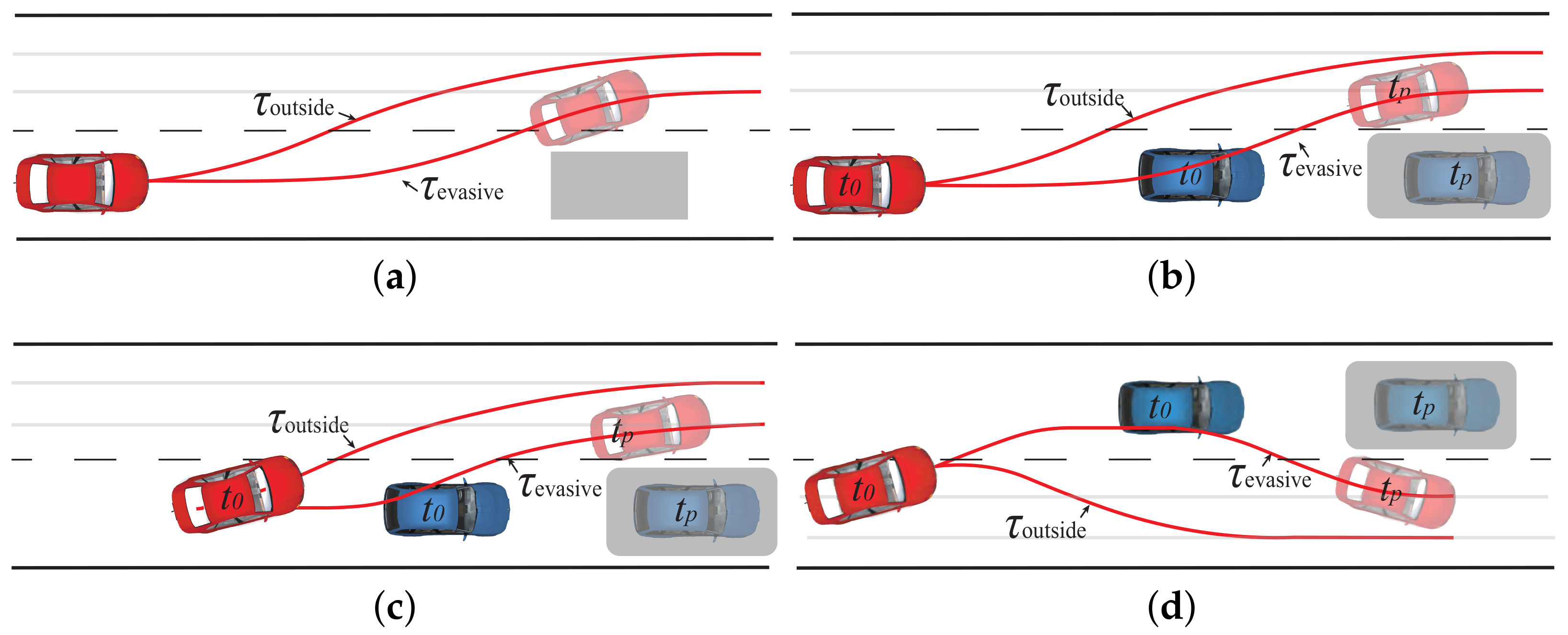
As shown in Figure 13, the path ${\tau }_{\mathit{o}\mathit{u}\mathit{t}\mathit{s}\mathit{i}\mathit{d}\mathit{e}}$ represents the boundary path of the driving envelope to arrive at the outermost safe lateral position, discussed in Section 3.2. Path ${\tau }_{\mathit{e}\mathit{v}\mathit{a}\mathit{s}\mathit{i}\mathit{v}\mathit{e}}$ represents the boundary path of the evasive maneuver to arrive at the innermost left lateral safe position. If the longitudinal position of the host vehicle is in range $[{\mathit{x}}_{\mathit{m}\mathit{i}\mathit{n},\mathit{s}\mathit{a}\mathit{f}\mathit{e}},{\mathit{x}}_{\mathit{m}\mathit{a}\mathit{x},\mathit{s}\mathit{a}\mathit{f}\mathit{e}}]$, we can get the trajectory ${\tau }_{\mathit{e}\mathit{v}\mathit{a}\mathit{s}\mathit{i}\mathit{v}\mathit{e}}$ which follows the evasive motion model, choosing the innermost safe lateral position as the target lateral position, and reaching the critical position defined in Section 2.3. If a dynamic front vehicle is driving forward, the extreme situation is defined as Figure 13b,c,d. The ${\tau }_{\mathit{e}\mathit{v}\mathit{a}\mathit{s}\mathit{i}\mathit{v}\mathit{e}}$ is considered as the most extreme trajectory that avoids collision with obstacles. The area ${\mathit{R}}_{\mathit{s}}$ under the constraint of steering limitation and road boundary has been obtained in Section 3.2. If no safe trajectory exists which meets both obstacle avoidance safety constraints and the steering limitation, the driving envelope does not exist. The driving envelope for evasive maneuver of a static obstacle is shown in Figure 13a. The driving envelope for lane-change maneuver is shown in Figure 13b,c. The driving envelope for lane-change abortion is shown in Figure 13d, the boundary path ${\tau }_{\mathit{e}\mathit{v}\mathit{a}\mathit{s}\mathit{i}\mathit{v}\mathit{e}}$ is composed of three parts, adjusting the lateral velocity to zero, following the direction of road, then performing evasive maneuver to arrive at the critical position.

4. The Applications of the Driving Envelope

4.1. Intervention Time

The proposed driving envelope can be utilized to determine the intervention time for semi-autonomous vehicles. The collision probability is used to determine the intervention time in [20]. The collision probability is computed by randomly generating N particles and computing the number of particles that collide with the traffic participants. Inspired by their work, we determine the intervention time for a human-in-the-loop shared driving system by calculating the probability of violating the safe driving envelope,

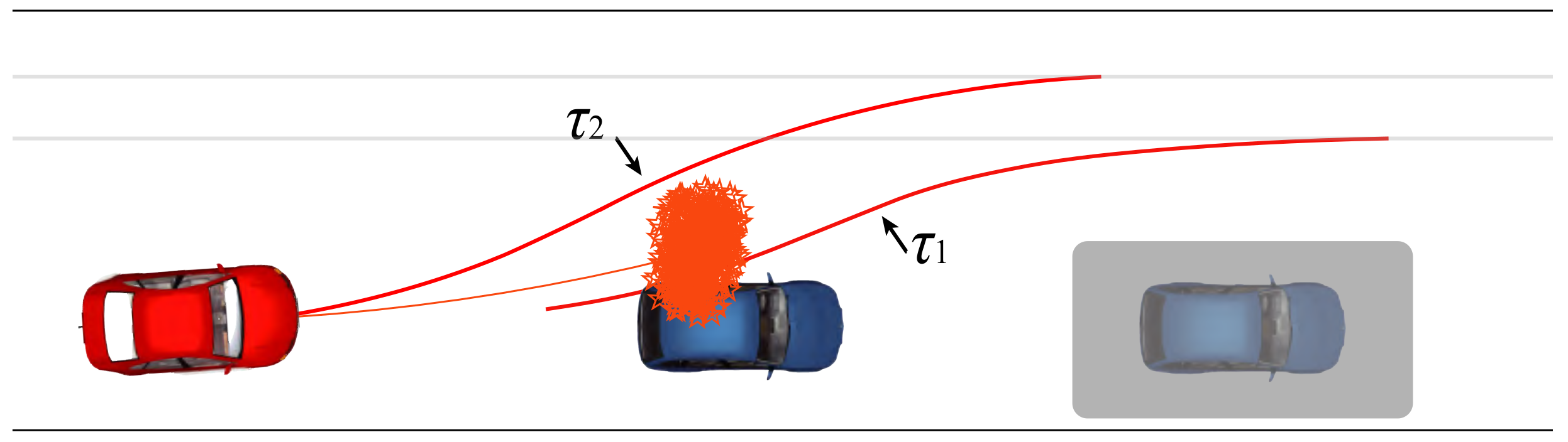
We predict the future occupancy set of the host vehicle at each time step by randomly generating N particles based on the driver’s input and vehicle state. The Constant Turn Rate and Acceleration (CTRA) kinematics motion model [38,39] is used to predict the state of the host vehicle in a short prediction horizon. By adding uncertainty to the control input, the possible occupancy set of each time step can be obtained. For example, the generated particles at 1.5 s are shown in Figure 14.

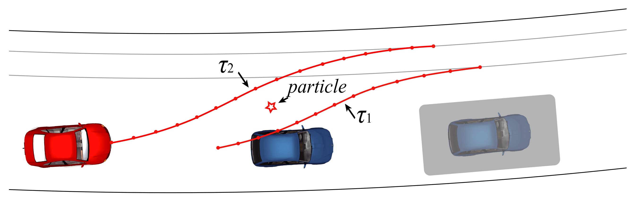
The driving envelope is generated considering the prediction time horizon. If one particle is outside of the generated driving envelope, then it can be treated as an unsafe state. The greater the probability of locating outside the driving envelope at a future time step, the greater the probability of arriving at an unsafe state. The probability of locating outside the driving envelope at each time step can be obtained by counting how many particles are outside of the driving envelope.

$${\mathit{p}}_{\mathit{o}\mathit{u}\mathit{t}\mathit{s}\mathit{i}\mathit{d}\mathit{e}}=\frac{{\mathit{N}}_{\mathit{o}\mathit{u}\mathit{t}\mathit{s}\mathit{i}\mathit{d}\mathit{e}}}{N}$$

(20)

where N is the total number of generated particles, ${\mathit{N}}_{\mathit{o}\mathit{u}\mathit{t}\mathit{s}\mathit{i}\mathit{d}\mathit{e}}$ is the number of particles distributed outside of the driving envelope. As shown in the Figure 14, the boundary paths of the proposed driving envelope are ${\tau }_1$ and ${\tau }_2$. If the lane is not straight, we convert the discrete points on boundary paths of the driving envelope from the reference frame into the cartesian coordinate, and connect the discrete points into line segments. Whether the point exceeds the safety zone is determined by judging which side of the line the point is on, as shown in Figure 15.

When ${\mathit{p}}_{\mathit{o}\mathit{u}\mathit{t}\mathit{s}\mathit{i}\mathit{d}\mathit{e}}$ at a future prediction time step reaches a predefined threshold, the shared driving system can provide warning or intervention. An advantage of this method is that it can guarantee the exist of collision avoidance trajectories when the system intervenes, and the system will not intervene too early.

4.2. Motion Planning

The driving envelope can be utilized in motion planning. The polynomial method is used to generate trajectories with kinematic constraints. Each trajectory is evaluated according to a cost function, which is designed considering the cost of path smoothness, safe distance to obstacles, etc [4,40]. The proposed driving envelope has been combined with the polynomial methods to generate a set of trajectories in our previous work [41]. The fifth-order polynomial for the lateral motion and the longitudinal motion in a reference frame is used to generate the trajectories.

$$\begin{array}{cc}\hfill \mathit{d}\left(\mathit{t}\right)=& {\mathit{c}}_5{\mathit{t}}^5+{\mathit{c}}_4{\mathit{t}}^4+{\mathit{c}}_3{\mathit{t}}^3+{\mathit{c}}_2{\mathit{t}}^2+{\mathit{c}}_1\mathit{t}+c_0\hfill \end{array}$$

(21a)

$$\begin{array}{cc}\hfill \mathit{s}\left(\mathit{t}\right)=& {\mathit{a}}_5{\mathit{t}}^5+{\mathit{a}}_4{\mathit{t}}^4+{\mathit{a}}_3{\mathit{t}}^3+{\mathit{a}}_2{\mathit{t}}^2+{\mathit{a}}_1\mathit{t}+{\mathit{a}}_0\hfill \end{array}$$

(21b)

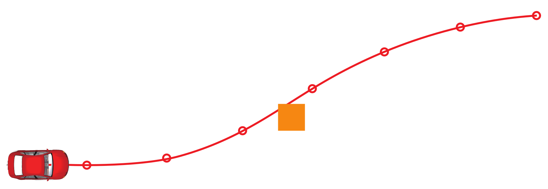
The coefficients ${\mathit{c}}_i(\mathit{i}=0,1,...5)$ and ${\mathit{a}}_{\mathit{i}}(\mathit{i}=0,1,...5)$ can be obtained according to the initial and terminal states in the reference frame. The points on each trajectory is generated according to Equation (21). When the sampling time is determined and the vehicle moves at a high speed, the distance between the generated points may be too far away for checking collision with obstacles, as shown in Figure 16. This problem can be avoided by decreasing sampling time, but the cost for generating the trajectories will increase. If the safe driving envelope is generated according to the obstacles, and trajectories are generated in the driving envelope, this problem will be solved.

An important parameter in the polynomial methods is the total time T used to move from the initial state to the terminal state. For each trajectory, the each component is generated by sampling the time t in total T. Generally, the T is also sampled, the invalid trajectories are deleted if the trajectories violate kinematic constraints, or collide with obstacles. Collision checking is time-consuming, which influence the computational efficiency of the polynomial methods [42]. In the worst case, collision check with every traffic participant and obstacle during all prediction horizon for each trajectory is needed. In the proposed driving envelope, the kinematic constraints and collision avoidance are already considered. By using the driving envelope, the time for collision check and constraint check will be reduced. In this paper, the motion model in Section 2.2 can be used to get the range of time $\mathit{T}\in \left[{\mathit{T}}_{\mathit{m}\mathit{i}\mathit{n}},{\mathit{T}}_{\mathit{m}\mathit{a}\mathit{x}}\right]$ for generating trajectories.

$$\begin{array}{cc}\hfill {\mathit{T}}_{\mathit{m}\mathit{i}\mathit{n}}=& {\mathit{t}}_{\mathit{a}\mathit{r}\mathit{r}\mathit{i}\mathit{v}\mathit{e}}-\mathcal{E}\hfill \end{array}$$

(22a)

$$\begin{array}{cc}\hfill {\mathit{T}}_{\mathit{m}\mathit{a}\mathit{x}}=& \mathit{m}\mathit{a}\mathit{x}({\mathit{t}}_{\mathit{m}\mathit{a}\mathit{x}},{\mathit{t}}_{\mathit{b}\mathit{o}\mathit{u}\mathit{n}\mathit{d}}+{\mathit{t}}_{\mathit{a}\mathit{r}\mathit{r}\mathit{i}\mathit{v}\mathit{e}}+\mathcal{E})\hfill \end{array}$$

(22b)

where ${\mathit{t}}_{\mathit{m}\mathit{a}\mathit{x}}$ is the predefined maximum time for T, $\mathcal{E}$ is a constant for tuning time T. Given the longitudinal velocity profile and the longitudinal distance ${\mathit{d}}_{\mathit{b}\mathit{o}\mathit{u}\mathit{n}\mathit{d}}$ from the current position to the boundary path of the driving envelope, ${\mathit{t}}_{\mathit{b}\mathit{o}\mathit{u}\mathit{n}\mathit{d}}$ is the time for longitudinal motion to arrive at the boundary path of the driving envelope. ${\mathit{t}}_{\mathit{a}\mathit{r}\mathit{r}\mathit{i}\mathit{v}\mathit{e}}$ is the time to move laterally to the target lateral position.

According to the relationship of the heading angle in reference frame and the target lateral position, there are three cases of calculating ${\mathit{t}}_{\mathit{a}\mathit{r}\mathit{r}\mathit{i}\mathit{v}\mathit{e}}$, as shown in Figure 17.

(1) Case I, the host vehicle is under the process of driving towards the target lateral position, and the host vehicle faces the direction of the target lateral position, as shown in Figure 17a. Given the current state in the reference frame, we can obtain the total time ${\mathit{t}}_{\mathit{l}\mathit{a}\mathit{t}}$ of lateral motion and the time ${\mathit{t}}_{\phi }$, which has been discussed in Section 2.3.2. The remaining time to finish the lateral motion is ${\mathit{t}}_{\mathit{a}\mathit{r}\mathit{r}\mathit{i}\mathit{v}\mathit{e}}={\mathit{t}}_{\mathit{l}\mathit{a}\mathit{t}}-{\mathit{t}}_{\phi }$.

(2) Case II, the host vehicle is under the process of driving away from the target lateral position, and the heading of the host vehicle faces the opposite direction of the target lateral position, as shown in Figure 17b. This case is similar to lane-change abortion maneuver discussed in Section 2.3.4. The evasive trajectory can be divided into two parts, ${\tau }_{\mathit{a}\mathit{d}\mathit{j}}$ and ${\tau }_{\mathit{e}\mathit{v}\mathit{a}}$. In the first part ${\tau }_{\mathit{a}\mathit{d}\mathit{j}}$, we assume that the vehicle moves at a constant lateral acceleration ${\mathit{a}}_{\mathit{l}\mathit{a}\mathit{t},\mathit{a}\mathit{d}\mathit{j}}$. The used time to adjust the lateral speed in the reference frame is ${\mathit{t}}_1={\mathit{v}}_{\mathit{l}\mathit{a}\mathit{t}}/{\mathit{a}}_{\mathit{l}\mathit{a}\mathit{t},\mathit{a}\mathit{d}\mathit{j}}$. In the second part, we assume that the trajectory follows the motion model in Equation (2). The H can be obtained, thus we can get the time ${\mathit{t}}_{\mathit{l}\mathit{a}\mathit{t}}$ using Equation (4). The total time to finish the lateral motion is ${\mathit{t}}_{\mathit{a}\mathit{r}\mathit{r}\mathit{i}\mathit{v}\mathit{e}}={\mathit{t}}_{\mathit{l}\mathit{a}\mathit{t}}+{\mathit{t}}_1$.

(3) Case III, the host vehicle is preparing for an evasive maneuver and has not started lateral motion, as shown in Figure 17c and Figure 17d. We assume that the trajectory follows the evasive motion model in Equation (2). Given the starting and target lateral position, the total lateral distance H can be obtained, thus we can get the time ${\mathit{t}}_{\mathit{l}\mathit{a}\mathit{t}}$ to arrive at the target lateral position using Equation (4), ${\mathit{t}}_{\mathit{a}\mathit{r}\mathit{r}\mathit{i}\mathit{v}\mathit{e}}={\mathit{t}}_{\mathit{l}\mathit{a}\mathit{t}}$.

After the range of parameter T is determined, the trajectories can be generated. The trajectories can be evaluated according to a cost function to obtain the suboptimal trajectory. The cost function is designed considering the smoothness of the trajectory, the distance to obstacles, the stability, etc. We have utilized the trajectory generation and evaluation method in a semi-autonomous driving system [41]. One advantage of the method is that the range of parameter T is determined, the motion planner can generate fewer trajectories. Another advantage of the method is that with the help of the driving envelope, the problem of missing collision checking with obstacles shown in Figure 16 can be solved.

5. Experiments

(1). The Longitudinal Distance Error of the Evasive Motion Model

The evasive motion mentioned in Section 2.2 is decomposed into lateral motion and longitudinal motion. To obtain the applicable scope of the evasive motion model, the longitudinal distance errors at different constant speeds have been calculated. We set H as 3.5 m, and ${\mathit{t}}_{\mathit{l}\mathit{a}\mathit{t}}$ as 5 s. The maximum lateral velocity can be obtained, which is about 1.4 m/s, so the velocity should be higher than 1.4 m/s. As shown in Figure 18a, when the vehicle moves at a constant speed, the longitudinal distance error decreases as the velocity increase. When velocity equals 2 m/s, the distance error is about 1 m. As shown in Figure 18b, the minimum speed is set 2 m/s, when the vehicle moves at a constant longitudinal acceleration, the distance errors at different initial longitudinal speeds and accelerations are calculated. When the longitudinal speed is higher than 2 m/s, the longitudinal distance errors are lower than 1 m, and the longitudinal distance error decreases as the speed increases.

(2). The Safe Longitudinal Position at Different State

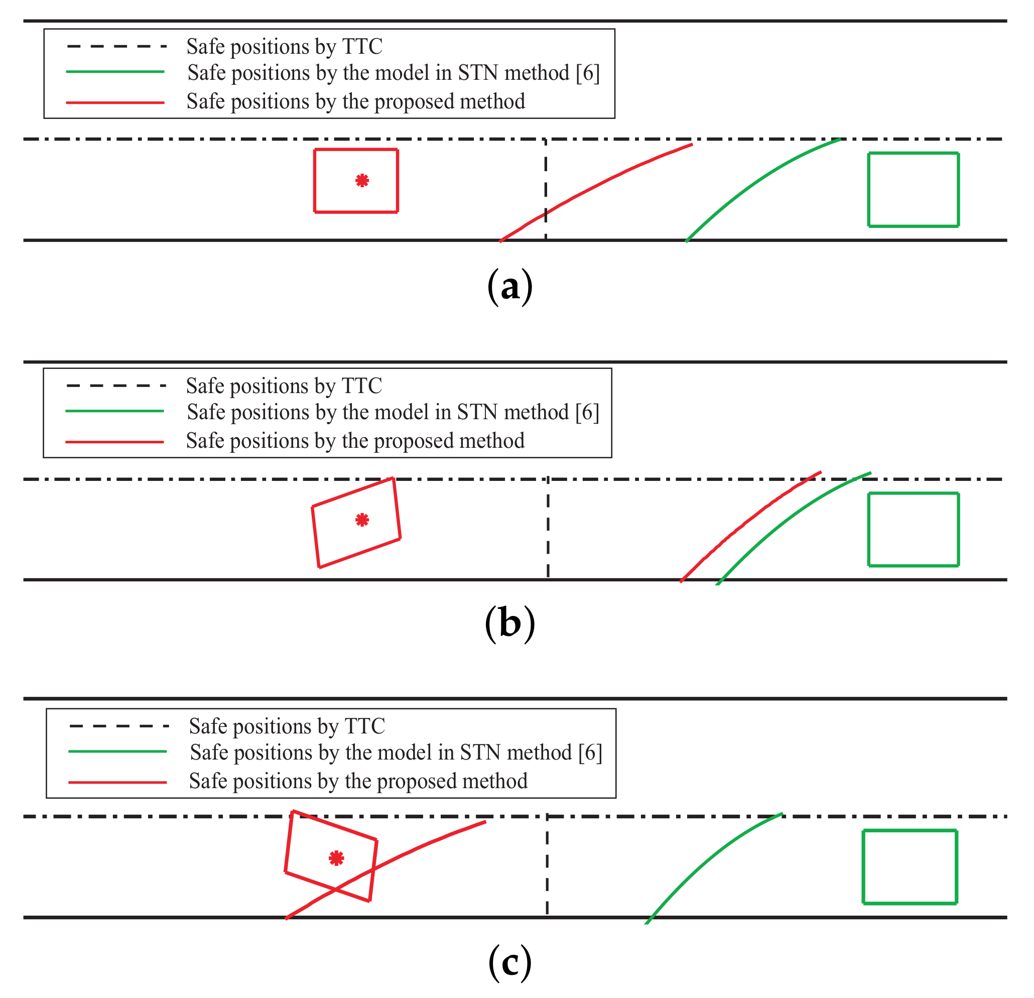
Given the allowed maximum lateral acceleration, the longitudinal safe position is influenced by the and the vehicle state. Taking the scenario of avoiding collision with a slow front vehicle ${\mathit{L}}_0$ as an example, as shown in Figure 19. The speed of the host vehicle is 20 m/s, the speed of the front vehicle is 15 m/s, the longitudinal distance between them is 30 m.

The safe distance for vehicle ${\mathit{L}}_0$ is denoted as ${\mathit{D}}_{\mathit{L}0,\mathit{s}}$. The maximum safe longitudinal position of the host vehicle ${\mathit{s}}_{\mathit{m}\mathit{a}\mathit{x}}={\mathit{s}}_{\mathit{L}0}-{\mathit{D}}_{\mathit{L}0,\mathit{s}}$. The longitudinal safe distance ${\mathit{D}}_{\mathit{L}0,\mathit{s}}$ at the different lateral positions can be calculated according to Section 2.3, and the safe position at each different lateral positions can be obtained.

As is shown in Figure 19, the red bounding box represents the host vehicle, the green bounding box represents the vehicle ${\mathit{L}}_0$. The red solid line represents the safe positions at the different lateral positions with the minimum safe distance proposed in Section 2.3, the maximum acceleration of the evasive model in Equation (2) is set as 0.9 m/s ${}^2$. The proposed method can reflect the influence of the lateral motion on the safety distance. The closer the vehicle is to the right lane marking, the farther the safe distance is required for the evasive maneuver. The vertical black dashed line represents the safe positions determined by TTC, the TTC threshold is set as 4 s. The TTC is obtained by dividing the relative distance by the relative speed. As shown in the figure, the TTC method cannot reflect the influence of the lateral motion. The green solid line represents the safe positions determined by the constant lateral acceleration motion model in [6], the constant lateral acceleration is set as 0.9 m/s ${}^2$. The shape of the green solid line is similar to the proposed method in this paper. However, the method in [6] is only used to calculate the safe distance to the front obstacles, the rear dynamic obstacles are not considered. In this paper, the distance to the rear dynamic obstacles can also be calculated.

(3). The Driving Envelope in Double-Lane Traffic Scenario

Taking the scenario of avoiding collision with a slow front vehicle ${\mathit{L}}_0$ as an example. The speed of the host vehicle is 20 m/s, the speed of the front vehicle is 15 m/s, the distance between them is 23 m. The boundary trajectories of the driving envelope for avoiding collision with the slow front vehicle is shown in Figure 20.

The red rectangle represents the host vehicle, the green rectangle represents the vehicle ${\mathit{L}}_0$. The dashed red line ${\tau }_{\mathit{p}\mathit{o}\mathit{s}\mathit{i}}$ denotes the safe position obtained according to the safe distance derived in Section 2.3, the solid red line ${\tau }_{\mathit{o}\mathit{u}\mathit{t}\mathit{s}\mathit{i}\mathit{d}\mathit{e}}$ denotes the boundary trajectory to arrive at the outermost lateral safe position, the solid blue line ${\tau }_{\mathit{i}\mathit{n}\mathit{n}\mathit{e}\mathit{r}\mathit{s}\mathit{i}\mathit{d}\mathit{e}}$ denotes the boundary trajectory to arrive at the innermost lateral safe position. The line ${\tau }_{\mathit{i}\mathit{n}\mathit{n}\mathit{e}\mathit{r}\mathit{s}\mathit{i}\mathit{d}\mathit{e}}$ starts from the corresponding point on line ${\tau }_{\mathit{p}\mathit{o}\mathit{s}\mathit{i}}$. From Figure 20, we can see that the driving envelope considers not only the safe distance to obstacles, but also the input of the driver. The driving can reflect the safety margin in the future.

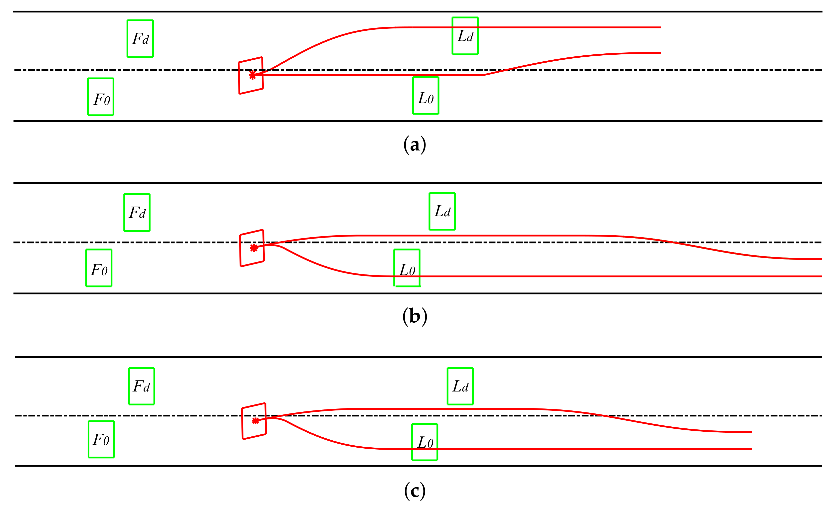
In a dynamic traffic scenario with four traffic participants ${\mathit{F}}_{\mathit{d}}$, ${\mathit{L}}_{\mathit{d}}$, ${\mathit{F}}_0$ and ${\mathit{L}}_0$, the driving envelope for a lane-change maneuver and a lane-change abortion maneuver is obtained as shown in Figure 21. The red bounding box represents the host vehicle, the green bounding boxes represent the traffic participants ${\mathit{F}}_{\mathit{d}}$, ${\mathit{L}}_{\mathit{d}}$, ${\mathit{F}}_0$ and ${\mathit{L}}_0$. The maximum lateral acceleration is set as 0.9 m/s ${}^2$ for evasive maneuver. When all vehicles are driving at 15 m/s, the driving envelope of continuing lane-change is shown in Figure 21a, the driving envelope of lane-change abortion maneuver is shown in Figure 21b. When the speed of vehicle ${\mathit{L}}_{\mathit{d}}$ is 5 m/s and other vehicles drive at 15 m/s, the safe distance constraint of lane change cannot be satisfied. Therefore, the driving envelope of continuing lane-change maneuver cannot be obtained. The safe distance constraint of lane-change abortion is satisfied, it’s safe to cancel lane-change, and the driving envelope of lane-change abortion is shown in Figure 21c.

The simulation is carried out in C++ using Intel I7-3520 CPU. In the traffic scenario shown in Figure 21, the CPU runs at 2.9 GHz, the average total time used to calculate the safe distance and generate the driving envelope for each driving maneuver is about 1 ms. The drivable area in [24] is represented as connected collision free convex sets. Owing to the consumption of computational resource, the computation time is 75 ms for time horizon 3 s on a 2.6 GHz Core, which is not enough for lane change in dynamic traffic flow. For the driving envelope generation method in [43], lots of points are generated, and the safety regions are computed using a Hamilton–Jacobi approach. When there are 70 longitudinal sampling points and 8 lateral sampling points, the calculation time is 34 ms. The above methods are very time-consuming. In order to use the methods in real-time applications, the time horizon has to be reduced.

In the experiment scenarios, the average total time for driving envelope generation is about 1 ms. The boundary paths of the reachable-set are generated to reflect the influence of the driver’s input and the steering limitation. The algorithm complexity of generating the boundary paths of the reachable-set is $\mathit{O}\left(\mathit{n}\right)$. In order to restrict the driving envelope within the road boundary, the evasive path to avoid collision with the road boundary, and the boundary paths of reachable-set are connected, as shown in Figure 12. The algorithm complexity for this path generation part is $\mathit{O}\left(\mathit{n}\right)$. The connection point is determined by searching the points on the two paths. The algorithm complexity for determining the connection point is $\mathit{O}\left(\mathit{n}\mathit{l}\mathit{o}{\mathit{g}}_2\mathit{n}\right)$. The safe distances for collision avoidance with obstacles are calculated. The path representing the boundary path of the obstacle evasive maneuver is generated from the minimum safe distance to the obstacle, as shown in Figure 13. The algorithm complexity for calculating the safe distance and generating the evasive path with the minimum safe distance to the obstacle is $\mathit{O}\left(\mathit{n}\right)$. Finally, the algorithm complexity of the driving envelope generation method is $\mathit{O}\left(\mathit{n}\mathit{l}\mathit{o}{\mathit{g}}_2\mathit{n}\right)$.

(4). The Real Vehicle Experiment

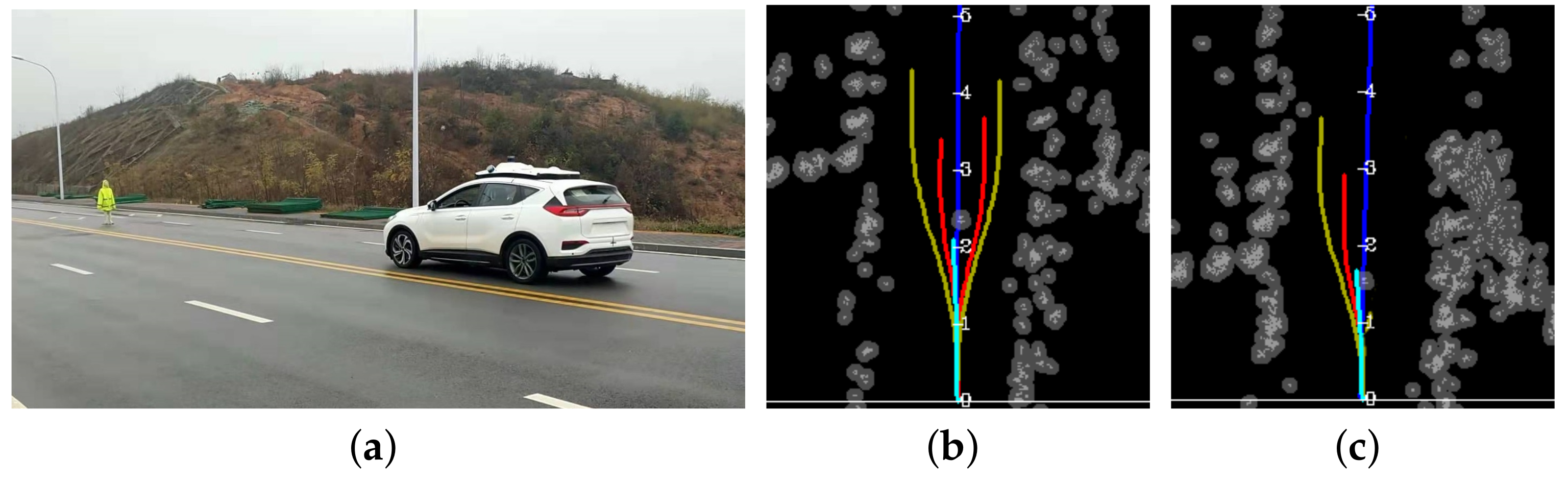
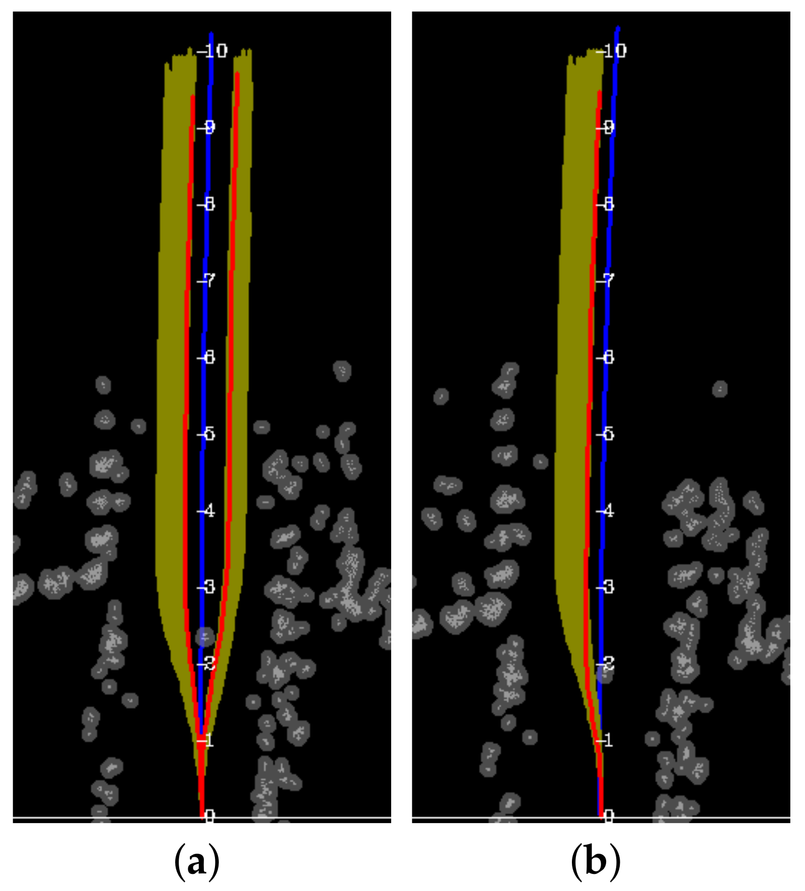
A modified Red Flag EHS3 based experimental platform was used to test the proposed driving envelope method. In the experimental driving scenario, a dummy was placed in the middle of the lane. A human drove the vehicle at about 20 km/h towards the dummy, as shown in Figure 22a. The driving envelope is used to determine the time for intervention and motion planning. The code is implemented in C++ using Intel I7-3520 CPU running at 3.3 GHz. The average total time used for calculating the safe distance and generating the driving envelope for both left side and right side evasive maneuver is about 1 ms. The generated driving envelope is shown in Figure 22b,c.

As shown in Figure 22b,c, the interval between the marks on the longitudinal axis is 10 m; the gray parts represent obstacles detected by Lidar; the black part is the non-obstacle area; the dark blue line denotes the reference path. The driving envelope is generated in the reference frame based on the reference path. The yellow lines denote the boundary paths to arrive at the outermost safe target lateral position, the red lines denote the boundary paths to arrive at the innermost safe target lateral position. The green line indicates the predicted trajectory for the next 3 s using the constant angular velocity and constant acceleration motion model without considering uncertainty.

Given the input and the state of the host vehicle, the feasibility of candidate evasive behavior can be identified quickly. At time ${\mathit{t}}_1$ shown in Figure 22b, the host vehicle can avoid collision from both the left side and the right side, and the driving envelopes for evasive maneuver from the both sides exist. At time ${\mathit{t}}_2$, only the driving envelope for the left side evasive maneuver exists, as shown in Figure 22c. The distance for right side evasive maneuver is not enough, it is not safe to drive from the right side of the dummy after ${\mathit{t}}_2$. When the probability of violating the driving envelope at the future time 1.5 s reaches 60 %, the semi-autonomous driving system intervenes. The generated trajectories and the suboptimal trajectories for the left-side and the right-side evasive maneuvers are shown in Figure 23. The yellow lines represent the generated trajectories, the red lines represent the selected trajectories for left-side and right-side evasive maneuvers. More detailed information on trajectory generation and evaluation methods are introduced in [41].

6. Conclusions

This paper introduced a novel driving envelope generation method for human-in-the-loop driver assistance systems. The driving envelope can be utilized to determine the safety of candidate driving maneuvers in real-time. The driver’s operation, the constraints of steering limitation, motion limitation, and collision avoidance are taken into consideration. The driving envelope can clarify the safe drivable area in the whole lateral evasive maneuver process. The efficiency of the proposed method is validated by simulation experiments and real vehicle tests. For the tested scenarios, the average total time to generate the driving envelope is about 1 ms. The driving envelope generation method proposed in this paper can be used in real-time applications. For future work, we will continue to study the method of combining decision-making and motion planning with the driving envelope.

References

- Chen, N.; van Arem, B.; Alkim, T.; Wang, M. A hierarchical model-based optimization control approach for cooperative merging by connected automated vehicles. IEEE Trans. Intell. Transp. Syst. 2020, 1–14. [Google Scholar] [CrossRef]
- Das, S.; Maurya, A.K. Defining Time-to-Collision Thresholds by the Type of Lead Vehicle in Non-Lane-Based Traffic Environments. IEEE Trans. Intell. Transp. Syst. 2020, 21, 4972–4982. [Google Scholar] [CrossRef]
- Hillenbrand, J.; Spieker, A.; Kroschel, K. A Multilevel Collision Mitigation Approach—Its Situation Assessment, Decision Making, and Performance Tradeoffs. Intell. Transp. Syst. IEEE Trans. 2007, 7, 528–540. [Google Scholar] [CrossRef]
- Keller, C.G.; Dang, T.; Fritz, H.; Joos, A.; Rabe, C.; Gavrila, D.M. Active Pedestrian Safety by Automatic Braking and Evasive Steering. IEEE Trans. Intell. Transp. Syst. 2011, 12, 1292–1304. [Google Scholar] [CrossRef] [Green Version]
- Jansson, J. Collision Avoidance Theory with Application to Automotive Collision Mitigation. Ph.D. Thesis, Linköping University Electronic Press, Linköping, Sweden, 2005. [Google Scholar]
- Nilsson, J.; Ödblom, A.C.; Fredriksson, J. Worst-case analysis of automotive collision avoidance systems. IEEE Trans. Veh. Technol. 2016, 65, 1899–1911. [Google Scholar] [CrossRef]
- Brunson, S.; Kyle, E.; Phamdo, N.; Preziotti, G. Alert Algorithm Development Program: NHTSA Rear-End Collision Alert Algorithm; Technical Report; U.S. National Highway Traffic Safety Administration: Washington, DC, USA, 2002. [Google Scholar]
- Noh, S.; Han, W.Y. Collision avoidance in on-road environment for autonomous driving. In Proceedings of the 2014 14th International Conference on Control, Automation and Systems (ICCAS 2014), Gyeonggi-do, Korea, 22–25 October 2014; pp. 884–889. [Google Scholar]
- Jula, H.; Kosmatopoulos, E.B.; Ioannou, P.A. Collision avoidance analysis for lane changing and merging. IEEE Trans. Veh. Technol. 2000, 49, 2295–2308. [Google Scholar] [CrossRef] [Green Version]
- Kaempchen, N.; Schiele, B.; Dietmayer, K. Situation Assessment of an Autonomous Emergency Brake for Arbitrary Vehicle-to-Vehicle Collision Scenarios. IEEE Trans. Intell. Transp. Syst. 2009, 10, 678–687. [Google Scholar] [CrossRef]
- Brannstrom, M.; Coelingh, E.; Sjoberg, J. Threat assessment for avoiding collisions with turning vehicles. In Proceedings of the 2009 IEEE Intelligent Vehicles Symposium, Xi’an, China, 3–5 June 2009. [Google Scholar]
- Li, X.; Sun, Z.; Cao, D.; He, Z.; Zhu, Q. Real-time trajectory planning for autonomous urban driving: Framework, algorithms, and verifications. IEEE/ASME Trans. Mechatron. 2015, 21, 740–753. [Google Scholar] [CrossRef]
- Bencloucif, A.M.; Nguyen, A.T.; Sentouh, C.; Popieul, J.C. Cooperative Trajectory Planning for Haptic Shared Control between Driver and Automation in Highway Driving. IEEE Trans. Ind. Electron. 2019. [Google Scholar] [CrossRef]
- Li, J.; Li, C.; Sun, Z.; Liu, D.; Dai, B.; Li, X. A Real-time Motion Planner for Intelligent Vehicles Based on a Fast SSTG Method. In Proceedings of the 2018 37th Chinese Control Conference (CCC), Wuhan, China, 25–27 July 2018; pp. 5509–5513. [Google Scholar]
- Kim, B.; Park, K.; Yi, K. Probabilistic Threat Assessment with Environment Description and Rule-based Multi-Traffic Prediction for Integrated Risk Management System. IEEE Intell. Transp. Syst. Mag. 2017, 9, 8–22. [Google Scholar] [CrossRef]
- Erlien, S.M.; Fujita, S.; Gerdes, J.C. Shared steering control using safe envelopes for obstacle avoidance and vehicle stability. IEEE Trans. Intell. Transp. Syst. 2016, 17, 441–451. [Google Scholar] [CrossRef]
- Cesari, G.; Schildbach, G.; Carvalho, A.; Borrelli, F. Scenario model predictive control for lane change assistance and autonomous driving on highways. IEEE Intell. Transp. Syst. Mag. 2017, 9, 23–35. [Google Scholar] [CrossRef]
- Liu, K.; Gong, J.; Kurt, A.; Chen, H.; Ozguner, U. Dynamic Modeling and Control of High-Speed Automated Vehicles for Lane Change Maneuver. IEEE Trans. Intell. Veh. 2018, 3, 329–339. [Google Scholar] [CrossRef]
- Lee, J.; Kim, B.; Seo, J.; Yi, K.; Yoon, J.; Ko, B. Automated driving control in safe driving envelope based on probabilistic prediction of surrounding vehicle behaviors. SAE Int. J. Passeng. Cars-Electron. Electr. Syst. 2015, 8, 207–218. [Google Scholar] [CrossRef]
- Shin, D.; Kim, B.; Yi, K.; Carvalho, A.; Borrelli, F. Human-Centered Risk Assessment of an Automated Vehicle Using Vehicular Wireless Communication. IEEE Trans. Intell. Transp. Syst. 2018. [Google Scholar] [CrossRef]
- Fraichard, T.; Asama, H. Inevitable Collision States. A Step Towards Safer Robots? Adv. Robot. 2004, 18, 1001–1024. [Google Scholar] [CrossRef] [Green Version]
- Lawitzky, A.; Nicklas, A.; Wollherr, D.; Buss, M. Determining states of inevitable collision using reachability analysis. In Proceedings of the 2014 IEEE/RSJ International Conference on Intelligent Robots and Systems, Chicago, IL, USA, 14–18 September 2014; pp. 4142–4147. [Google Scholar]
- Sontges, S.; Althoff, M. Determining the Nonexistence of Evasive Trajectories for Collision Avoidance Systems. In Proceedings of the 2015 IEEE 18th International Conference on Intelligent Transportation Systems, Gran Canaria, Spain, 15–18 September 2015; pp. 956–961. [Google Scholar]
- Söntges, S.; Althoff, M. Computing the Drivable Area of Autonomous Road Vehicles in Dynamic Road Scenes. IEEE Trans. Intell. Transp. Syst. 2018, 19, 1855–1866. [Google Scholar] [CrossRef]
- Shia, V.A.; Gao, Y.; Vasudevan, R.; Campbell, K.D.; Lin, T.; Borrelli, F.; Bajcsy, R. Semiautonomous vehicular control using driver modeling. IEEE Trans. Intell. Transp. Syst. 2014, 15, 2696–2709. [Google Scholar] [CrossRef]
- Driggs-Campbell, K.; Govindarajan, V.; Bajcsy, R. Integrating Intuitive Driver Models in Autonomous Planning for Interactive Maneuvers. IEEE Trans. Intell. Transp. Syst. 2017, 18, 3461–3472. [Google Scholar] [CrossRef]
- Driggs-Campbell, K.; Dong, R.; Bajcsy, R. Robust, informative human-in-the-loop predictions via empirical reachable sets. IEEE Trans. Intell. Veh. 2018, 3, 300–309. [Google Scholar] [CrossRef] [Green Version]
- Noor-A-Rahim, M.; Liu, Z.; Lee, H.; Khyam, M.O.; He, J.; Pesch, D.; Moessner, K.; Saad, W.; Poor, H.V. 6G for Vehicle-to-Everything (V2X) Communications: Enabling Technologies, Challenges, and Opportunities. arXiv 2020, arXiv:2012.07753. [Google Scholar]
- Bagheri, H.; Liu, Z.; Lee, H.; Pesch, D.; Moessner, K.; Xiao, P. 5G NR-V2X: Towards connected and cooperative autonomous driving. arXiv 2020, arXiv:2009.03638. [Google Scholar]
- Ni, J.; Hu, J.; Xiang, C. Envelope control for four-wheel independently actuated autonomous ground vehicle through AFS/DYC integrated control. IEEE Trans. Veh. Technol. 2017, 66, 9712–9726. [Google Scholar] [CrossRef]
- Kritayakirana, K.; Gerdes, J.C. Autonomous vehicle control at the limits of handling. Int. J. Veh. Auton. Syst. 2012, 10, 271–296. [Google Scholar] [CrossRef]
- Brännström, M.; Sandblom, F.; Hammarstrand, L. A probabilistic framework for decision-making in collision avoidance systems. IEEE Trans. Intell. Transp. Syst. 2013, 14, 637–648. [Google Scholar] [CrossRef]
- Xu, G.; Liu, L.; Ou, Y.; Song, Z. Dynamic modeling of driver control strategy of lane-change behavior and trajectory planning for collision prediction. IEEE Trans. Intell. Transp. Syst. 2012, 13, 1138–1155. [Google Scholar] [CrossRef]
- Bertolazzi, E.; Biral, F.; Da Lio, M.; Saroldi, A.; Tango, F. Supporting drivers in keeping safe speed and safe distance: The SASPENCE subproject within the European framework programme 6 integrating project PReVENT. IEEE Trans. Intell. Transp. Syst. 2010, 11, 525–538. [Google Scholar] [CrossRef]
- Shalev-Shwartz, S.; Shammah, S.; Shashua, A. On a formal model of safe and scalable self-driving cars. arXiv 2017, arXiv:1708.06374. [Google Scholar]
- Jiang, B.; Li, X.; Zeng, Y.; Liu, D. A Maneuver Evaluation Algorithm for Lane-Change Assistance System. Electronics 2021, 3, 774. [Google Scholar] [CrossRef]
- Jo, K.; Lee, M.; Kim, J.; Sunwoo, M. Tracking and Behavior Reasoning of Moving Vehicles Based on Roadway Geometry Constraints. IEEE Trans. Intell. Transp. Syst. 2016, 18, 460–476. [Google Scholar] [CrossRef]
- Schubert, R.; Adam, C.; Obst, M.; Mattern, N.; Leonhardt, V.; Wanielik, G. Empirical evaluation of vehicular models for ego motion estimation. In Proceedings of the 2011 IEEE Intelligent Vehicles Symposium (IV), Baden-Baden, Germany, 5–9 June 2011; pp. 534–539. [Google Scholar]
- Houenou, A.; Bonnifait, P.; Cherfaoui, V.; Yao, W. Vehicle Trajectory Prediction based on Motion Model and Maneuver Recognition. In Proceedings of the 2013 IEEE/RSJ International Conference on Intelligent Robots and Systems, Tokyo, Japan, 3–7 November 2013; pp. 4363–4369. [Google Scholar]
- Glaser, S.; Vanholme, B.; Mammar, S.; Gruyer, D.; Nouvelière, L. Maneuver-Based Trajectory Planning for Highly Autonomous Vehicles on Real Road With Traffic and Driver Interaction. IEEE Trans. Intell. Transp. Syst. 2010, 11, 589–606. [Google Scholar] [CrossRef]
- Jiang, B.; Li, X.; Zeng, Y.; Liu, D. Human-Machine Cooperative Trajectory Planning for Semi-Autonomous Driving Based on the Understanding of Behavioral Semantics. Electronics 2021, 10, 946. [Google Scholar] [CrossRef]
- Werling, M.; Kammel, S.; Ziegler, J.; Groell, L. Optimal trajectories for time-critical street scenarios using discretized terminal manifolds. Int. J. Robot. Res. 2012, 31, 346–359. [Google Scholar] [CrossRef]
- Xausa, I.; Baier, R.; Bokanowski, O.; Gerdts, M. Computation of avoidance regions for driver assistance systems by using a Hamilton–Jacobi approach. Optim. Control Appl. Methods 2020, 41, 668–689. [Google Scholar] [CrossRef]
Figure 1.
The lateral motion of the evasive motion model. The dashed blue line and red solid line respectively represent the values by setting as 5 s and 3 s.
Figure 2.
The position of vehicle during the lane-change process.
Figure 3.
The safe distance for lane-keep maneuver.
Figure 4.
The safe distance of evasive maneuver for static obstacle. (a) The extreme trajectory of evasive maneuver using evasive motion model. (b) The critical position of evasive maneuver.
Figure 5.
A lane-change scenario in double-lane highway.
Figure 6.
The critical situations for lane-change considering uncertainty of prediction. (a) The critical situation for at . (b) The critical situation for at . (c) The critical situation for at . (d) The critical situation for at .
Figure 7.
The minimum and maximum longitudinal position for lane-change scenario.
Figure 8.
The stages for lane-change abortion. (a) The first case, the host vehicle cancels the lane-change maneuver in a lane-keep mode. (b) The second case, the host vehicle cancels the lane-change maneuver in a lane-change mode.
Figure 9.
The defined critical lateral position for a right lane-change scenario. (a) The lateral position for vehicle at . (b) The lateral position for vehicle at . (c) The lateral position for vehicle at . (d) The lateral position for vehicle at .
Figure 10.
The minimum and maximum longitudinal position for lane-change abortion.
Figure 11.
The reachable set with different initial curvature . (a) . (b) . (c)
Figure 12.
The reachable-set area and the driving envelope considering road boundary.
Figure 13.
The driving envelope for lane-change and lane-change abortion. (a) The driving envelope for collision avoidance of static obstacle. (b) The driving envelope for lane-change before lateral movement. (c) The driving envelope for lane-change during lateral movement. (d) The driving envelope for lane-change abortion.
Figure 14.
The generated particles and the driving envelope.
Figure 15.
One generated particle and the driving envelope in the reference frame.
Figure 16.
Collision checking for an obstacle.
Figure 17.
The different cases of calculating . (a) The vehicle faces the direction of the target lateral position. (b) The vehicle faces the opposite direction of the target lateral position. (c) The vehicle is preparing for a left side evasive maneuver. (d) The vehicle is preparing for a right side evasive maneuver.
Figure 18.
The longitudinal distance errors of the evasive motion model. (a) The distance errors at different constant speeds. (b) The distance errors at different accelerations.
Figure 19.
The safe positions for avoiding collision with the front vehicle. (a) . (b) . (c) .
Figure 20.
The boundary trajectories for avoiding collision with a slow front vehicle. (a) The boundary trajectories of lane-change maneuver, . (b) The boundary trajectories of lane-change maneuver, . (c) The boundary trajectories of lane-change maneuver, .