
The Ability to Control VOC Emissions from Multilayer Building Materials


Department of Thermal Physics, Acoustics and Environment, Building Research Institute, 00-611 Warsaw, Poland
*
Author to whom correspondence should be addressed.
Appl. Sci. 2021, 11(11), 4806; https://0-doi-org.brum.beds.ac.uk/10.3390/app11114806
Submission received: 18 March 2021
/
Revised: 30 April 2021
/
Accepted: 21 May 2021
/
Published: 24 May 2021
(This article belongs to the Special Issue New Challenges for Indoor Air Quality)
Abstract
:The work aimed to investigate which parameters of the electrically powered radiant floor heating system are connected with the intensity of VOC total emissions and emissions from individual layers, which can be effectively changed and controlled to obtain energy savings in the ventilation process. For this purpose, experimental studies of VOC emissions from specially designed LRFHS samples (Laboratory Radiant Floor Heating System) were carried out, along with simulations of real thermal conditions of samples of layered systems containing separate heaters and various materials layers. The TD-GC-MS chromatography was used to assess the trends of VOCs concentration changes in 480 h in a test chamber (simulating real conditions) for several LRFHS systems of multilayer construction products with built-in individual heating systems, in two stabilised temperatures, 23 °C and 33 °C, two stabilised relative humidities, 50% and 80% and three air exchanges per hour ACH on levels 0.5, 1.0 and 1.5. The obtained results indicate that the models used to determine emissions from single-layer products correspond to the description of emissions from multilayer systems only to a limited extent; some inner layers of floor systems are giving diffusion resistance or intensification of diffusion. A new emission model is proposed. The time-emission concentration curves for dry and wet environments differ significantly; reducing the VOC concentration in the air for the number of exchanges above 1.0 ACH is relatively inefficient. Authors also mapped out new research directions; for example, the experiment showed that not all of the VOC contaminants are ventilated just as easily and perhaps, considering their concentration of resistant impurities, chemical structure and diffusion resistance through the layers, there is a need to determine their weights.
1. Introduction
1.1. General Overview of the Research Problem
Indoor air quality (IAQ) continues to be a major environmental problem due to the presence of indoor pollutants and their health hazards, irritation and discomfort to occupants. Volatile organic compounds (VOCs) are one of the main indoor air pollutants [1], and their excessively high concentration in rooms affects the well-being and health of users, which can cause Sick Building Syndrome (SBS) [2], defined as a complex of disease symptoms occurring in a building. The source of volatile organic compounds is, among others, construction products containing organic solvents or polymers. Often, their presence in the room is indicated by a chemical smell, which can be irritating. An unpleasant odour’s perception increases with the increase in temperature caused by solar radiation or during the heating season when ventilation in the rooms is limited [3,4]. In the flooring systems used in apartment construction and offices, numerous construction products are used, often characterised by significant VOC emissions, e.g., adhesives or primers. The indoor air pollution level related to VOC’s air concentration, apart from the emissions from products, depends on many factors such as air humidity, number of air changes and temperature [4]. Heated floors, covered by the authors′ current research interest, are a special case, where higher temperatures may significantly increase emissions, especially in the first few days after installation. The authors discovered also that the assessment of the VOC emission level from multilayer systems in the context of the variability of environmental parameters is a seldom-described issue in the literature. In the case of many layers of products in the floor system, diffusion resistance causes emission delay in time and non-obvious waveforms. Our research consideration is that the models used to determine the air pollutant concentration from a product with a single layer can only partially be used to assess complex product systems, e.g., floors. Standardised test methods for VOC emissions from construction products do not consider temperature effects from underfloor heating systems [5]. An example of this is the horizontal research standard EN 16516, which assumes standard conditions for testing products at a temperature of 23 °C ± 1 °C.
Typical VOC emission testing is based on assessing the concentration of chemical compounds emitted from the building material in the test chamber based on a European model room’s assumption reflected in the standardised test chamber [5]. The test conditions are specified in the standards EN ISO 16000-9: 2006 [6], including test temperature, minimum chamber area, its tightness, airflow range, chamber structure andthe number of air changes per hour. For example, in the literature data, Fortmann [7] and Kozicki [8] present experiments completed at one temperature, 23 °C. The dominating research work in literature is focused on the evaluation of formaldehyde determined by the HPLC method and the assessment of the total volatile organic compounds, TVOC (Total Volatile Organic Compounds), by the GC/MS (Gas Chromatography with Mass Spectrometry) method and less frequently, the measurements of the concentrations of individual compounds in the C6–C16 range.
Considering the lack of published research on the emissions from multi-product systems (as in our case–the electrically heated floors) considering the variability of the environmental conditions with increased temperature and humidity, the authors planned, developed and provided a series of laboratory experiments where such dependence is investigated using a modified chamber method based on the standard approach [5].
A large number of construction and finishing materials have emerged that emit volatile substances as organic compounds (VOCs) are commonly used in buildings, including adhesives [9], carpets [10], floorings [11], ceiling tiles, paints and furniture [12,13,14]. Throughout their use, these materials emit a large number of different pollutants especially with a high concentration peak shortly after their installation. The authors consider the fact that these emissions may increase highly with an increase of indoor temperature.
Accurate models predicting indoor VOC emissions are essential for determining indoor pollutant concentrations and occupant exposure. Only on the basis of knowledge about the complex physical processes of emissions, it is possible to justify the correct choice of the form of the analytical model, which would not only refer to already proven analytical models (see Section 2.1) of emissions and contain selected emission parameters but also fit the measured VOC emission time courses. Such models must have a solid basis in the form of experimental research.
In our case, on the basis of provided experimental VOC air concentration tests (considering higher temperature and humidity), the authors propose a new model C(t) of VOC concentration in test chambers with heated floors.
1.2. State of Knowledge–Emission Modelling
In order to make basic assumptions about the shape of the VOC emission model and its components for heated floors (considering a higher temperature and humidity), it is necessary to present the existing state of the art on emission modelling. Based on a provided review in this section, the authors in the next section, Methods, propose a model that is used later to determine the VOC concentration regression profiles based on the experimental results (VOC emission test in chambers).
The prediction of VOC concentration in a chamber or room is attempted by modelling carried out on the basis of the analysis of the influence of variables, e.g., temperature, air humidity and air change rate on the characteristic parameters of the physical processes of emission: initial VOC concentration in solid material (µg m−3), diffusion factor of a given VOC in the emitting building material Dm (m2/s) and the dimensionless mass partition coefficients Kma of the diffusing agent into the part of the mass remaining in the porous material and the part of the mass released into the environment above the emitting surface. These parameters are the output of models of convergence of heat diffusion and the VOC migration processes in porous materials (single and multilayer, dry and wet environments).
Existing emission models typically fall into one of the following types: empirical, analytical or mass-transfer-equation-based. The literature analysis suggests the need to refine this division of models considering verified assessments of their reliability, the possibility of generalisation and the ease of use in practice, leading to the presentation of their classification proposals (see Figure A1, Appendix A).
The first group of publications contains five basic publications on emission models based on the theory of mass transfer of VOC compounds from building materials, in which models of the first researchers of emission phenomena from a single homogeneous layer and a double layer are presented. Little et al. [10] first presented an emission analysis with a model to predict diffusion-controlled VOC emissions from homogeneous building materials. Although the model is useful and straightforward in many cases, an extension of the assumption neglecting convective mass transfer resistance through the air boundary layer was not justified under all conditions. This model’s parameters were the initial VOC concentrations in the material, the material–air partition coefficient and the material’s VOC diffusion coefficient. The presented model has been verified by comparing it with the carpet emission tests results and analysing the determined model parameters′ influence on the emission profile runs. Cox et al. [11] used this analytical model to calculate the emission rate of vinyl flooring and found a relatively good agreement. Based on the model of Little et al. [10], Zhao et al. [12] developed an analytical model to study the transition state and reproduce the reversible effect of secondary adsorption as a response to the simultaneous emissions of pollutants. Huang and Haghighat [13] developed a numerical model taking into account the mass transfer resistance by introducing mass transfer coefficients; however, they assumed that the VOC concentration in the air should be zero in the gas phase.
Xu and Zhang [14] presented an improved model that overcame the two previous models′ limitations and obtained an analytical solution. However, as the authors′ reserve, Xu and Zhang’s solution is not fully analytical because it is coupled with the air concentration and needs to be solved simultaneously.
Later, Deng and Kim [15] developed a fully analytical solution of the given system of Xu and Zhang’s equations [14]. The Deng model was later the most frequently cited and left the largest trace in the existing models of physical VOC emission processes from building materials. The Deng Kim model [15] takes into account both material diffusion and mass transfer through the air boundary layer. As the authors themselves claimed, a general characteristic equation is developed which would reduce to that of Little et al. [10] when the gas phase mass transfer coefficient becomes infinite. The Deng Kim model [15] shows a good agreement with the experimental data, while the model of Little overestimated the concentration of the emitting VOC in the air.
When building their model, used until today, Deng Kim [15] needed basic parameters of the mass transfer process, i.e., they used the experimental data of mass transfer: the diffusion coefficients of VOCs Dm in the materials, the initial concentrations in the materials Co and the material–air partition coefficients Kma (verified by the CFD method) from Yang et al. [16]. Another study by Huang Haghighat [17] looked at the effect of air velocity on the amount of emissions (measured as chamber C(t) in the air) due to an increase in the VOC diffusion coefficient in the material. For a material with a diffusion coefficient Dm > 10–10 m2/s, the VOC emission rate increased with increasing velocity, with air velocity having a significant effect on VOC emissions. For a material with a diffusion coefficient of Dm < 10−10 m2/s, the VOC emission rate increased with the increase in air velocity only in a short period of time <24 h. The source publications in the diagram (Figure A1, Appendix A) show reference to the research by Yang [9] and the more recent publication by Xiong, Huang and Zhang [18], which describes a new quick method for measuring two key parameters, Kma and Dm, as well as convective mass transfer coefficient (hm). Compared to traditional methods, it has the advantage that the Kma, Dm and hm factors can be obtained in one experiment simultaneously, making it convenient to use. The frequently cited research on the theoretical dependence of the VOC emission rate from building materials on temperature was carried out by the team of Xiong, Wei, Huang and Zhang [19] focused on the example of formaldehyde. Their validated correlation “shows that the logarithm of the emission rate by a power of 0.25 of the temperature is linearly related to the reciprocal of the temperature”. The emission rate at temperatures other than the test condition can be obtained using the correlation, greatly facilitating engineering applications. However, theoretical work on the procedures for determining the parameters of physical emission models is still ongoing. For example, Liu, Nicolai et al. [20] used the Least Square and Global search algorithm with multi-starting points to achieve a good agreement in the normalised VOC concentrations between the model prediction and experimental data. They estimated the effects of experimental uncertainty of chamber-measured concentration.
Returning to the work of the Deng Kim [15] team, their new approach was based on the fact that they adopted some known empirical relations for the determination of the mass transfer coefficient in the gas phase. For laminar flow, it was assumed [13] (1):
where Sh = hl/Da is Sherwood’s number, Sc = ν/Da is Schmidt’s number, Re = ul/ν is Reynolds’ number, ν is the kinematic viscosity of air, u is the velocity of air above the material, l is the characteristic length of the material, Da is the VOC diffusion coefficient in the air and h is the gas phase mass transfer coefficient (m·s−1).
Apart from these uniform initial condition models, Kumar and Little [21] also developed a model for the two-layer system with the assumption thatan initial condition is given by a general non-uniform concentration profile in each material layer. This model was useful for studying the effects of adopting different initial VOC concentrations in the emitting layers. Two years later, the team of Qian [22], based on the solution (Deng and Kim [15]) and the equations derived from dimensionless analyses by Xu and Zhang [14], normalised these equations and obtained a group of dimensionless correlations for VOC emissions from dry building materials. The team of Qian [22] showed that the time dependence of the dimensionless quantity characterising quantitatively the emission (total VOC mass emitted per unit area of building material at time t (mg m−2) and the time dependence of the dimensionless quantity characterising the total emission rate (depending on the VOC emission rate per unit area of building material at time t (mg m−2 s−1) are functions of only four (not seven, as according to Deng, Kim [15]) dimensionless parameters, i.e., the ratio of the mass transfer number to the partition coefficient (Bim/Kma), the Fourier number (Fom), dimensionless air change number coefficient (α = Nδ2/Dm) and the ratio of building material volume to chamber volume or room volume (β = Aδ/V). With these correlations, the emission rate could be easily estimated. In addition, the team of Qian et al. [22] determined experimentally expected ranges of values of dimensionless parameters useful in the fitting procedures, e.g., emission rates in time using the least-squares method.
In recent years, too often, ventilation systems provide nominal airflow rates regardless of the actual need for dilution. In this way, there will be more cold air in the heating season that needs to be heated to ensure thermal comfort, which increases heat loss through ventilation. An effective way to reduce these heat losses through ventilation is to install an intelligent ventilation system, which is characterised by the possibility of continuous adaptation of ventilation, which consequently leads to energy savings without lowering the air quality IAQ. One application of intelligent ventilation systems is demand-controlled ventilation (DCV). In the past, most DCV systems only considered CO2 and H2O as good indicators of comfort, ignoring the other VOC emitting contaminants that determine the health aspects of IAQ. New systems may include: (1) a thermal model; (2) a ventilation airflow model and models of selected pollutants levels. However, the condition for the use of intelligent ventilation systems is the availability in databases of the characteristics of materials emitting in various hygro-thermal conditions of the environment. Then, the emission parameters Dmi and Coi parameters for the i-th emitting material enter the system as input data for the model. Such a model for the emission source, which is a layer of building material with a thickness of δ, with the diffusivity Dm (variable depending on air temperature and humidity) and the initial concentration C0 of volatile VOC gases in the material (variable depending on temperature and absolute air humidity), was developed by De Jonge and Laverge [23]. The difficulties in applying this model are that the reference emission data was poorly available (the model excluded the partition coefficient Km).
The problem of evaluating the impacts of VOC emissions from building materials on the indoor pollution load and indoor air quality beyond the standard chamber test conditions and test period, with the use of mechanistic emission source models, was recognised by two research teams, Liu et al. [20] and Rode et al. [24].They co-worked with Project IEA EBC Annex 68,”Indoor Air Quality Design and Control In Low Energy Residential Buildings” (completed in 2020). Scientific research may involve an explanation through the mechanistic description. Mechanisms comprise entities, the physical actorsof a system, and activities that the entities perform. These entities and activities are then organised temporally and spatially in such a way as to give rise to the overarching behaviour of the mechanism [25].The project considered the problem to provide a comprehensive set of data and tools whereby buildings′ indoor environmental conditions can be optimised. Research teams of Liu et al. [20] developed a procedure for estimating the mechanistic emissions model parameters using VOC emission data from standard small chamber tests.
In the second group of models presented in the literature (see Figure A1, Appendix A), models are also presented, partly based on the theory of mass transfer, but these are specialised models of VOC emissions from systems of multilayer building materials; these systems in our research report are very important because the subject of these studies were multilayer sets of products-emitting VOCs, representing as faithfully as possible the practical sets of floor layers. Although our discussion’s subject is currently emission models from multilayer systems, the researchers from Lawrence Berkeley National Laboratory, Hodgson, Wooley, Daisey [26] should be considered a precursor. However, their research is limited to providing the captured elapse time emission curves of several compounds. Such tests were performed by observing the emissions from one layer of solid material (in this case, a carpet), but in fact, it was a two-layer system in which the double layer was represented by material/air interface.
As a result of this work, volatile VOC emission profiles from several new carpets were recorded. More comprehensive was the research carried out at Concordia University by Haghighat, de Bellis [27]. Their scope can be included in the same group of observation of phenomena, although there is a reference to the physical model according to Fick’s second law and the related need to diversify the description of emission phenomena:
where δCa/δt is a rate of change in the concentration of compound a (mg/m3 h−1), Dm = diffusion coefficient (m2/h) and ∇2 = the Laplacian operator of Ca (concentration of compound a in the overlying air (mg/m3). Each compound under given environmental conditions has its own diffusion coefficient, depending on its molecular weight, molecular volume, temperature and the material’s characteristics within which the diffusion occurs.
Haghighat and Huang [28], followed by Zhang Niu [29] and Kim et al. [30], continued their work, now on a physical model of a multilayer material based on the theory of mass transport, although, according to other authors [31,32], it is not possible to develop such a model. This would be a model from which the final concentration of VOC emitted from the surface of a multilayer sample could be determined by simply superimposing the concentrations of pollutants emitted from the individual layers of building materials. This is not possible because the model uses four parameters specific to each material of each layer: the diffusion coefficient of each material layer (Dm,i), material/air partition coefficient for each material layer (Kma,i), initial concentration in each material layer (C0,i) and convective mass transport coefficient (hma). Such a model would ignore the phenomenon of mutual suppression of VOC diffusion through layers.
The models are to be used to predict the rate of VOCs emission from a multilayer material: the rate of VOCs absorption by the material, the concentration of VOCs in the air, both emitted from VOC sources and materials post-adsorbing (sink) VOC gases from the surrounding air (Cair–chamber concentration) and the spatial distribution of VOC concentration within the material. Typical layered building materials are in the form of composites such as wall-layering systems (paint/plasterboard/water vapour insulation) or floor-layering systems (wax/vinyl/adhesive/concrete). The model validation results [28,29,30,31,32] showed that the multilayer material exhibits the same or similar emission properties as the top layer material. The top layer strongly retards the emission of VOCs from the bottom layer material. A multilayer material has a much longer VOC emission time than a single-layer material.
Deng et al. [32] investigated the influence of the multilayer material system’s parameters on VOCs emission. The results showed that the inner layer could act as a VOC adsorbent or emission source to the top layer depending on the initial VOC concentration in thelayer’s material. In the case that the inner layer is an emission source for the outer layer, the outer layer becomes a barrier layer reducing the rate of VOC emission from the source.
The emission profile characteristic determined experimentally for the layered building material was presented by Weigl et al. [33]. TVOC emissions from OSB wood-based boards and the same boards covered with gypsum fibreboards (GKF boards) were investigated. VOC emissions from uncoated OSBs were higher in the beginning. In the presented case, the maximum (TVOC concentration peak in emission profile) was reached after 3 days, followed by a sharp decrease in the emission profile curve in the time period until the seventh day of the measurement, in which the second decay curve breaking down and a slow but continuous decrease of emissions until the end of the experiment could be read. Considering both curves of the emission profile, it can be stated that the gypsum covering the surface of the OSB board caused a reduction and significant delay in the first peak of TVOC concentration.
Another approach to building a model of emissions from many coexisting emitting surfaces in one space, which also applies to layered building materials systems, is presented by Guo et al. [34]. When different building materials release VOCs at the same time, the indoor VOC concentration increases and vice versa decreases due to the mutual inhibition of the emissions released from the material. Therefore, the whole process is dynamic, and the final indoor VOC concentration cannot be obtained by simply superimposing the concentrations of pollutants emitted from the individual layers of dry building materials [31]). An equation describing the equilibrium of mass transfer through all thin layers of material [34] would be Equation (3):
where V is the chamber volume (m3), Ca is the concentration of compound a in the overlying air (mg/m3), Q is the amount of ventilating air, m3 h−1, Ai is the emitting surface of the i-th building material, m2 and Dm,1 is the diffusion coefficient of the compound transfer through the material a of the lower layer with a thickness of δ1 of the layer system, Dm, and diffusion factor of the compound a through the material of any layers i. However, this equation does not take into account the mutual inhibition effect of emissions and assumes constant values of Cm,i,; therefore, it would only be valid at very short intervals. For the numerical determination of the time course of the increase in the concentration of VOC in the chamber caused by the emission of VOC from building materials coexisting in the chamber (in the floor layers), Guo et al. [34] used the finite difference method (Saul’ev finite difference method). They validated the model in the testing of chamber VOC emissions from wall and floor sandwich systems. Interestingly, for both models, in the Deng and Kim physical model completed in 2004 [15] based on mass transfer equations and the Guo et al. model [34], the same assumptions were made.
The third group of models provided in the literature (Figure A1, Appendix A) is related to the emission from wet materials. When considering the study of emissions from wet material, it should be emphasised that the generally accepted definition of wet material is a solid, homogeneous material covered with a layer of liquid coating. Furthermore, for such materials, the Yang et al., [35] models were built, which take as a variable the thickness of the liquid’s emitting top layer. As demonstrated by testing VOC emissions from liquid coating materials in a small test chamber in accordance with standard ASTM D 5116−06 [36], the emission profile consists of two stages: an early stage (stage I), during which the material is still quite wet, has a high emission level whichdecays quickly and another dry stage (stage 2) during which the VOCs are released much more slowly [35]. Rapid emission occurs mainly by evaporation from the surface of the material, with internal diffusion relatively negligible at this early stage, while in the subsequent dry stage, internal diffusion becomes the controlling factor. Usually, there is a transitional phase between the two steps, which makes the prediction of VOC emissions from liquid materials more complicated. Studies by Yang et al. [35] and Haghighat and Huang [28] have shown that the emissions of “wet” materials will depend on environmental conditions (e.g., temperature, air velocity, turbulence, humidity and VOC concentration in the air), as well as the physical properties of the material and the substrate (e.g., diffusivity). Since many factors can influence the emission behaviour of “wet” materials, testing of emissions by laboratory experimentation is usually necessary and expensive (time-consuming).
Altkinkaya [37] built an emission model from a single homogeneous layer of wet material that accommodates this layer’s changing thickness during emission and considers both internal and external mass transfer resistances through the moving wet shell/air interface. However, the simplifying assumptions introduced, related to the assumption of homogeneity of the wet material layer (constant Cm and Kma values of the wet layer), limit this model’s scope of application.
A frequently cited work by Deng, Zhang and Qiu, [38] presents a model of emission from a moist material with thickness varying during the emission process. This model is not exponential but expressed by a fairly simple differential equation, the variable of which is the thickness of the material layer, but its solution is complicated by the adopted variables (reduction) of the Cm values (VOC concentration in the material) as well as the partition coefficients Kma. Therefore, in multilayer systems, the Deng equation for emissions from wet materials would be difficult to use by a difficult mathematical model because the Deng, Zhang and Qiu [38] equation is solved using the generalised integral transform technique (GITT).
All the above-mentioned mathematical models of emission processes are troublesome to use, although they were created to predict the rate and mass balance of emissions from building materials of different structures and physical conditions. Moreover, it is also difficult to find a relationship between the models. The experimental VOC emission characteristics are inconvenient for engineering applications due to the relatively slow emission rates under chamber test conditions. Therefore, it remains to simulate emission processes, which is related to the need to develop simpler models.
The fourth group of publications (Figure A1, Appendix A) presents analytical models for the simulation of VOC emissions from building materials. For example, the Deng Kim [15] model’s mass transfer model parameters have a practical application for understanding the mechanism of VOC emissions′ physical processes from building materials. However, these parameters usually involve additional physical parameter measurements needed to perform a simulation using the model. Consequently, it is crucial to establish a simple and practical model to predict building material emissions.
Research on the development of analytical models for engineering applications was carried out assuming constant values of the emission rate of pollutants or assuming that the concentration of TVOCs at the boundary of building material is exponentially decaying (adopted constantly, e.g., concerning formaldehyde HCHO emissions).
The ASTM D 5116-06 Standard Guide [36] is important in this group of publications (Small-Scale Environmental Chamber Determinations of Organic Emissions From Indoor Materials/Products) based on a study by Tichenor, Sparks and Jackson [39] (of which the emission profile is cited in Figure A1), which proposes an analytical model useful in calculating the VOC chamber concentration during an emission test. The model includes the exponential equation to calculate the emission factor EF and the chamber concentration Ci of the VOC emitting from a material/product sample in a small, normalised chamber used in the standard chamber test. This model, called the first-order decay source model, is one of the most frequently used models of empirical emission processes carried out in a ventilated chamber (small-scale Environmental Test Chamber). The ASTM 5116-06 Standard Guide [36] presents the first-order decay source model C(t) with the following solution under the condition of t = 0 and C = 0:
where C is chamber VOC concentration (mg m−3), N is air change rate (h−1), L is chamber loading factor (m2·m−3) and k is first-order decay rate constant (h−1). EF0 is the initial emission factor from the equation (in mg m−2 h−1) calculated in the formula:
where EF (ti)–emission factor at time ti and ΔCi/Δti—the slope/gradient of the time concentration curve at time ti (h). This model was also adopted in a simplified form. As a result of the research carried out at the LBNL in Berkeley (Willem [40] and Hodgson et al. [41]) on the optimisation of the strategy of removing air pollutants in residential residences, it was found for most VOC compounds (except, e.g., formaldehyde) that if the emission factor EF (t) was constant, the emitted VOC concentration in rooms/chambers was inversely proportional to the time-averaged air-change rate. Therefore, the equation simplified by Willem et al. [40] for constant source is adopted in the following form:
where EF is emission factor mg m−2 h−1; A is floor surface m2; V-is chamber volume m3; N is air change rate h−1, Cout is outdoor VOC concentration mg m−3 and C is chamber VOC concentration mg m−3; t-time h.
Two recently published analytical models of emissions were developed in 2020 by two Chinese scientists’ teams with a very similar composition Zhang, Niu, Liu et al. [42] and Zhang, Liu, Wu et al. [43]. These are exponential mass transfer models that eliminate some of the disadvantages of the empirical model, and their parameters have a justified reference to the parameters of physical models. Efforts were made to develop a practical and straightforward model to simulate the VOC emission characteristics in an environmental chamber, taking into account convective mass transfer and equalising mass balance in the indoor environment. The mass transfer model considers the release characteristics of formaldehyde and VOCs from the following three aspects: (1) VOCs diffuse in materials, (2) diffusion from the surface of building materials to the air boundary layer, and (3) convection and diffusion of the air layer. According to both models, the concentration of Cair in the environmental chamber can be expressed:
where,
where Kma is an interface partition coefficient of TVOC between the material and the interface, h is the convective mass transfer coefficient m h−1and B is constant. The authors of the model Zhang, Niu, Liu et al. [42] ignored the process of filling the environmental chamber with TVOC without chemical reactions, Equation (13), which allowed to simplify to the following exponential decay model:
The authors of the model Zhang, Liu, Wu et al. [43] ignored only the chemical reactions during the emission process and wrote the equation as an empirical model of decay of emissions doubly exponential in the form:
This very analytical model of the double exponential decay empirical model became an inspiration for the new emission model described in this paper, with the additional assumption of trying to eliminate the partition parameter Kma from the equation of the physical value, which would be difficult to determine in a multilayer floor system composed of several materials.
It should also be added that the authors are aware of the potential and possible use of finite element program (CHAMPS) for a thermodynamic VOC equilibrium modelling also in a multilayer structure. In recent years, FDFD methods were used for research on heat and moisture transfer in construction and the selection of parameters of thermal insulation layers of partitions, also for heated wall units, e.g., [44]. The authors are interested in applying the FDFD method to the selection of layer parameters in the close future.
1.3. The Research Issues Discussed in the Study
There are numerous publications that investigate the influence of environmental parameters on VOC emission from products mostly on the building level, for example, [45,46]. However, so far, no research team has analysed this issue by a chamber method for multilayer product systems where the heat source is built into the system of the emitting products. The basic thesis of the presented research was to demonstrate the significant influence of temperature on the emission from the multi-layer heated floor systems based on a chamber test.
The need for research on the influence of temperature and humidity on emissions from products is demonstrated, for example, in the publication [45], with the intention to scale up and validate emission models from chambers held at constant conditions to actual buildings.
The foundation of our research presented in this paper was the examination of emission of VOC profiles from multilayer construction products with a laboratory radiant floor heating system (LRFHS) in a chamber with a set of different environmental conditions. The VOCs concentrations in a time of 480 h were assessed under variables of three airflow rates (n = 0.5, 1 and 1.5), three temperatures (23, 29 and 33 °C) and two humidity (RH) levels (50% and 80%). Several variations of LRFHS samples with various multilayer structure were selected (dry and wet type) and prepared to determine the time-concentration VOC emissions profiles, using an environmental test chamber according to ASTM D 5116-06 [36]. The chamber method was used with a newly designed innovative ceramic housing allowing to test samples of multi-layered floor systems electrically heated.
The experimental VOC chamber concentration results were used to determine the component parameters of the proposed emission model (see Section 2.1) and the emission regression line (trend profiles of C(t) (17)) from each floor system under different boundary conditions. In addition, the authors found that the model adequate to one layer should be enriched with the original delay parameter.
This research paper takes into consideration and provides:
- -
- A comprehensive literature review on the emission models’ types;
- -
- The conditions and rules for conducting the experiment, i.e., research on changes in VOC emissions profiles over time from representative systems of multilayer construction products used in heating floors under changing boundary (environmental) conditions;
- -
- A prototype of laboratory stand, the universal system for testing VOC emissions from multilayer building partition systems was built;
- -
- Studies of the influence of temperature, humidity and the number of air changes on the emission from several multilayer systems (wet and dry conditions);
- -
- A justified model of emission from multilayer product systems with a new delay factor (compared to models from single-layer systems) based on experimental results and theory;
- -
- A discussion of results.
2. Materials and Methods
2.1. Emission Modelling Proposal
In order to determine the VOC emission profiles from heated floors in time based on the experimental results, the authors propose the following approach and model. The emission factor may be calculated as follows:
where EF is the emission factor (µg/m2/h), C is the chamber’s air concentration (µg/m3), n is the ventilation air change (h’1) and L is the loading factor (m2/m3).Based on studies, the following emission model is proposed:
where R1 is the component of the emission factor connected to the desorption process and R2 is the component connected with diffusion. R01 and R02 are the initial emission factors, and k1 and k2 are the specific coefficients that account for the decrease in emission concentrations during the time of the test, respectively. R1 is considered to reflect a desorption process from a floor system’s surface, whereas R2 is considered to reflect a diffusion process in a multilayer floor system. Factors k1 and k2 are the coefficients in h−1 that account for the decrease in emission rate during the test. The coefficients k1 and k2 are also used for each system, and numerical methods determine each experiment’s boundary conditions. k1 and k2 were assumed to have values that were independent of any particular VOC. When adsorption onto chamber walls and inflow impact from outdoors is negligible, the mass balance of a test chamber according to composed of components is also presented in the literature (ASTM D 5116-06) and can be described as follows:
where C(t) is the concentration of VOC (in µg/m3) at time t (h). Substituting Equation (12) for Equation (13), assuming an initial VOC concentration of zero, provides the following test chamber concentration decaying model:
The authors investigated this model by comparing simulation results with actual indoor air concentration-by-time sequences in a test chamber. The R01 and R02 coefficients are calculated on the basis of the results of laboratory tests of VOC in the chamber in practice, using the formulas:
and
where ∆C1 (µg/m3) is the difference between the maximum concentration of VOC (in µg/m3)assessed in the chamber and the initial concentration in the chamber at time 0, ∆t1 is the time to reach the maximum VOC concentration in the chamber from time 0, ∆C2 is the difference between the second curve breakpoint concentration of a VOC (µg/m3) assessed in the chamber and the final concentration in the chamber at time 480 h and ∆t2 is the time to reach the final VOC concentration in the chamber from the time of the second curve breakpoint.
As the authors found out on the basis of preliminary analyses, model (14), composed of elements presented in the literature (ASTM standard, also see Section 1.2), better reflects the nature of emissions from single-layer products. In our case, due to several layers of multilayer floor products and the upper layer (ceramic tiles, wooden “parquet” panel), the standardised approach gives only sufficient traceability with the obtained results—the potential trend lines coincide very moderately with the model for one layer (without the use of the emission delay factor). The VOC concentrations in the chamber found in the tests are delayed in relation to those resulting from the model (14). This results directly from the diffusion resistance of the multilayer floor system. Therefore, the authors finally decided to introduce into Equation (14) the original delay term X, hereinafter referred to as the Piasecki–Kostyrko factor. Equation (14), along with the original delay factor X, takes the following new form:
where:
where a and b are the coefficients selected experimentally with numerical methods so that the determination factor R2 of the new model (17) and experimental points of VOC concentration C(t) were the highest possible (0.7–0.95). In Equation (18), the coefficient a from the delay term X takes in practice (as presented in Results) the value from 0.45 to 0.55 in our model fittings. The delay component reaches the value close to one in the time for the highest VOC concentration during the test. In most cases, the coefficient b is not necessary (as a correction only) and takes the value 0. Adopting such a retarder term X eliminates the non-realistic maximum concentration peaks resulting from the earlier model (14), especially for higher air humidity RH = 80% in a test chamber.
X = a log(t) + b
The aim of the experimental tests is to determine the component parameters of the model (17) to determine the emission concentration regression curves over time in accordance withthe experimental results. Finding the optimal solution for a function with three parameters a, k1 and k2 is not a task requiring advanced numerical techniques. The numerical method the authors used assumes the search for a, k1 and k2 that would give the highest R2 coefficient for the comparison of the C(t) model and VOC concentration experimental points. In order to search for the optimum, a sequence of numbers of a, k1 and k2 was generated (corresponding to the Monte Carlo method), which are successively substituted into the equation C(t), and R2 was calculated for each iteration. When the value of the variability of a single parameter gives R2 optimum, the sequence of numbers for the next parameter is generated near the value of the first R2 optimum. A three-dimensional space is created which usually has a few optimums, from which we choose the best (with three assigned parameters).In practice, the range of the values of a, k1 and k2 are more or less known, so the sequence of iteration seeking the R2 optimum does not have to be very long (several dozen operations for each sample).
2.2. Selection of Construction Products
In order to select products for testing the emission of volatile organic compounds, an analysis of the market-available construction of floor heating systems used in real solutions was carried out. The construction products located under the top layer of the heating floor, through which the heat passes, were selected for the test. The products to be tested include primers, waterproofing products and adhesives for wood and ceramic floors. The products were selected, taking into account their chemical composition achieved by testing VOC emission from single products (Table 1). Most of them were based on polyurethane or epoxide resins with solvent, a significant VOC emission source. According to the technical documentation provided by the manufacturers, products can be used indoors.
2.3. The Electrically Powered Radiant Floor Heating System LRFHS–Selected Laboratory Samples
LRFHS simulates the floor’s real conditions with a radiant floor heating system, taking into account the relationship between the heater’s temperature and the temperature of the top surface of the floor. In order to assess the VOC emission characteristics of construction products used, the chamber tests were carried out for dry (leaving room, bedroom simulation) and wet rooms (bathroom simulation). The construction practice (e.g., EN 1264) indicate the permissible temperature of the floor surface layer of the heated floor. The temperature for residential and office spaces should not exceed 29 °C, and for wet rooms (e.g., bathroom), it should not be higher than 33°C. On this basis, two types of working conditions were simulated by the authors for the study of VOC emissions from construction products used with the radiant floor heating system: dry (type D) and wet (type W). For D-type rooms, the surface layer’s maximum temperature, which was an oak parquet of 29 °C, was assumed. In the case of W-type rooms, the top layer was ceramic tiles, and their maximum temperature was 33 °C. It was assumed that the humidity RH for D-type simulation will be 50%, and for W rooms, 80% (in a test chamber). The test results for W and D simulations were compared with the room test conditions without floor heating (23 °C and 50% or 80% RH). Two types of samples were prepared for the testing of emissions of volatile organic compounds corresponding to the conditions in dry (type D) and wet (type W) simulations. The sample structure was based on the installation scheme of the heating floor layers, shown in Figure 1.
The floor heating sample was located in a ceramic housing made of 10 mm thick fibre-cement sheets. The properly cut sheets pieces were connected with each other by means of screws so as to form a cuboid open at the top. One wall of the housing wasunscrewed/opened in order to introduce subsequent layers of the sample. The use of ceramic housing of the sample packaging allowed the authors to obtain thermal inertia which allowed for better thermal stabilisation of the system. It also has slots where high-quality temperature sensors T1, T2 and T3 were inserted between the sample layers. The outer walls of all samples in the ceramic housings were additionally protected with aluminium foil against possible VOC emission from the side walls or joints at the final stage of preparation. The surface area of the base of the ceramic housing and each of the layers was 0.04 m2. It was set so that a chamber loading factor L—the ratio of the test specimen area to the chamber volume of product—was 0.4 m2/m3, which is the test-recommended value for products used for floors in accordance with the EN 16516 standard [5].
The fixed layers of the sample, permanently built into the ceramic housing of the sample regardless of type D or W (Figure 2), placed on the bottom of the structure, are thermal insulation (floor polystyrene, 30 mm), a ceramic tile (4 mm) and an electric heater as presented in Figure 3 cross-section of the sample types D and W).
A concrete block with a thickness of 6 cm, corresponding to the concrete floor screed, was placed on the heater. It was prepared in a special form in accordance with the EN 12390-2 standard. Process thermometers shields were placed at the bottom and top of the mould to insert temperature sensors during the emission tests, and the concrete blocks were seasoned for 28 days after formation. The basic element of the emitting sample was a multilayer of under-floor construction products, different for samples of type W and D. For D samples (Figure 4), it was always the set of primer and wood adhesive coating covered by oak parquet, which was the same two layers for all samples. For W samples (Figure 5), it was always the primer, waterproofing and ceramic adhesive coating covered by ceramic tiles, which was filled by cement fugue, the same three layers for all samples.
Sets of construction products for the study of volatile organic compounds emissions from a multilayer of underfloor construction products are presented in Table 2 and Table 3.
Each set was applied on a concrete block according to a technical sheet within 24 h and a concrete block covered by a multilayer system was placed on a flat thermal radiator.
2.4. Experimental System
A special laboratory test stand was designed and developed to conduct the experiment. The experimental system contained a stainlesssteel chamber, a clean air generator, an air preparation system and a Laboratory Radiant Floor Heating System (LRFHS) electrically powered with a temperature regulation and monitoring unit (Figure 6).
The test chamber was connected with an electronic mass flow controller controlling the airflow and air-change rate. During the experiment, the air exchange rate n was 0.5 h−1 for one test period, 1.0 h−1 for a second test period and 1.5 h−1 for a third test period. The air velocity above RFHS was set within the range of 0.1 m/s to 0.3 m/s. Sensors measured the temperature (Tchamber) and relative humidity of air RH in the ventilated chamber. The volume of the chamber is 0.1 m3.The main elements of the LRFHS are the heater, the temperature control and a monitoring system with temperature sensors controlling the temperature of the top layer surface (T1), multilayer coating (T2) and heater (T3). The task of the LRFHS was to maintain the set temperature of the top surface layer (T1) equal to 29 °C for samples and 33 °C for W samples. The optimal heater temperature value (T3) was 40 °C for the D samples and 45 °C for the M samples. The heating system is equipped with nine calibrated sensors, PT-100. These are resistance sensors made of platinum with a resistance value of 100 Ω at 0 °C. Two types of sensors were used: Type 361 with a length of 15 cm and a diameter of 2.5 mm is placed in the process cover, which will enable its multiple-use, Type 383 with a diameter of 30 mm × 3.5 mm and a thickness of 1.5 mm.
The authors designed an experiment comparing the nature of the emission of volatile organic compounds from the multilayer construction products under standard conditions equal to 23 °C (without heating) and heating for dry or wet rooms. Tests were carried out simultaneously in twochambers with temperature values of 23 °C and 29 °C (for dry D samples) or 33 °C (for wet W samples). The given test parameters are presented in Table 4.
The stability of temperature detected during the monitoring test chamber time (emission profile time) is presented in Figure 7. Stabilised temperature variations T1 and T2 are bigger for wet samples W than for dry samples D but did not exceed 2 °C.
2.5. Sampling
Tests were carried out for three floor systems for dry rooms (D) and three multilayer systems for wet rooms (W). The tests for each system were carried out in parallel in two laboratory chambers: in the first with the conditions tested for a given room, in the second chamber for standard conditions. The floor temperature (T1) for D simulation was 29 °C, and the heater temperature was 40 °C with an indoor air humidity of about 50%. In the case of wet rooms, the floor temperature (T1) was 33 °C, with aheater temperature of 45 °C and air humidity in the chamber of 80%. The main air pollutants were obtained as a result of the chromatographic tests of air samples taken from the research chambers.
The tests were performed from the beginning of 2018 to the second half of 2020 practically all the time due to a large number of samples (approx. 600 air/VOC samples taken in the chamber) and 480 h test times for the one-floor system under two RH conditions (RH = 50% or RH = 80%) and two temperature conditions (23 °C and 29 °Cor 33 °C) with and without electric heating.
To sample VOCs, the chamber air outlet channel was connected with a Tenax TA tube (SUPELCO, US, Bellefonte, PA, USA). The sample was collected at a rate of 167 mL/min for 0.5 h using a GilAir Plus pump (Gilian, St. Petersburg, FL, USA). The experiment was conducted for 480 h for each test. During the first week, samples were taken several times a day, with the frequency of sampling being reduced as the tested compounds′ concentration stabilised. As far as possible, samples were taken at the following times after hours 0, 1, 2, 4, 6, 8, 10, 24, 28, 48, 52, 120, 124, 144, 168, 194, 218, 290, 314, 338, 362, 454, 459 and 480.
2.6. VOC Identification
The VOCs compounds were analysed by using the thermal desorption-gaschromatography-mass spectrometry detection technique (TD-GC-MS). A thermal desorption TD 20 (Shimadzu, Tokyo, Japan) and a GCMS-QP2010 Shimadzu (Tokyo, Japan) chromatograph were used for this purpose. The VOCs absorbed on Tenax TA were thermally desorbed. The tubes were heated at atemperature of 300 °C for 10 min under a helium flow (60 mL/min), and the substances were focused at −15 °C. The volatile compounds were injected into the GC capillary column by heating the cold trap to 280 °C for 5 min. The splitless injection mode was applied. The process of separation and analysis of volatile compounds was on a capillary column Restek RXI–5 (30 m, 0.25 mm ID, 1.0 µm df). The following GC oven temperature program was applied: initial temperature of 40 °C for 2 min, 10 °C per min to 260 °C with a final temperature of 260 °C for 3 min. Helium was used as the carrier gas. The MS analysis was carried out over a scan range of 30–500 m/z within ionisation energy of 70 eV in electron ionisation mode. The volatile compounds were identified on the basis of the retention time (see Figure A2 in Appendix A) and by mass spectrum, database search using the NIST 2011 spectral database (NIST, Washington, DC, USA). The concentration of the determined compounds was calculated on the basis of the curves of the standard solutions (LGC Standards GmbH, Washington, DC, USA). Standard compounds purity was greater than 99.5%.
3. Results and Discussion
3.1. Comparative Analysis of VOC Emission Test Results from Samples of Layered Floor Systems with a Surface Temperature of 23 and 33 °C in a Wet Indoor Environment W with a Surface Temperature of 23 and 29 °C in a Dry Indoor Environment D with ACH at 0.5 h−1, 1 h−1 and 1.5 h−1
First, the authors analysed the dependence of emission profiles for W- and D- type multilayer systems on the number of air changes 0.5 h−1, 1 h−1 and 1.5 h−1 in the test chamber.The TVOC emission profiles from W3 sandwich floor systems (tested for 480 h) for three air changes rates at 23 °C and RH = 80% in the test chamber are provided in Figure 8. Figure 9 shows the effect of the number of air changes on the TVOC concentration value in the chamber at 33 °C and RH = 80% for the W3 floor system (sequence of layers: Concrete → Primer → Waterproofing → Adhesive → Tile). For the experimental points of TVOC concentration in the test chamber obtained using the laboratory method, appropriate coefficients k1 and k2 were selected for the C(t) model (17) and the fitted lines were developed by numerical methods and the determination coefficient R2.
The values of the k1 coefficients for the C(t) model (17) are in the range 0.011–0.014 and k2 in the range 0.001 to 0. 0016. It is proven that the chamber’s air change rate had a direct effect on TVOC concentration values. For 33 °C, the change in the number of exchanges from n = 0.5 to n = 1 reduced the TVOC concentration by more than two times, and for 23 °C, the change in the number of exchanges from n = 0.5 to n = 1.5 resulted in a decrease in the concentration in the chamber by more than three times. In both cases, 23°C on Figure 8 and next for 33 °C in Figure 9, a greater decrease in concentration is observed when increasing the chamber’s number of air changes from n = 0.5 to n = 1, then decreases exponentially (with lower efficiency).
There is a clear influence of chamber temperature on the value of emissions from the floor system (in high humidity) and the chamber’s TVOC concentration. For the number of exchanges n = 0.5 over the entire course of 480 h, the concentration value at 33 °C was over two times higher than at 23 °C. For the number of exchanges n = 1, the concentration value is 80% to 40% higher for the temperature of 33 °C than at 23 °C during the test period of 480 h. It is also clearly visible that the maximum concentrations are achieved 24 to 30 h after inserting the floor system into the chamber. The delay of emissions in high humidity chambers in comparison to dry conditions will be discussed later. The difference in the course of Figure 8 and Figure 9 is that a temperature of 23 °C tends to create a peak in the course of the profile; at a lower temperature, it is much smaller. At lower temperatures, the retardation of the peak is greater, and it is connected to the fact that the lower are diffusion coefficients D.
The next two Figure 10 and Figure 11 show the same test condition for an experiment as for W3, but for the D1 sample at a lower temperature of 29 °C and lower humidity RH = 50% (D type, dry rooms); later, the same system is analysed for 23 °C. The D1 sample has a layer sequence: Concrete → Primer → Adhesive → Oak parquet and is composed of products described in Table 1 and Table 2.
The regression profiles C(t) fits and the R2 coefficient ranges from 0.61 to 0.94 (Figure 10). The values of the k1 coefficients for the C(t) model are in the range 0.01–0.023 and k2 in the range 0.001 to 0.002. For the D1 system (dry conditions, 29 °C), similarly to the W3 wet conditions, the same trend of TVOC in time was found; the TVOC concentration in the chamber decreases as the number of exchanges in the chamber increases.
The curve fits by providing that the model is just satisfactory, and the R2 coefficient ranges from 0.77 to 0.78 (Figure 11). In the case of a flow of n = 1, the experimental points do not follow the typical C(t) curve. In the authors’ opinion, this is most likely due to the test method uncertainty (~24%). However, for this non-obvious experimental trend, the authors set a curve based on a proposed model with R2 equal to 0.78.The values of the k1 coefficients for the C(t) model are in the range 0.002–0.009 and k2 in the range 0.0012 to 0.0013. As for the W3 samples at 23 °C, the trend towards a peak in the profile D1 at a lower temperature is lower.
An increase in TVOC concentration ΔCmax (µg m−3) caused by an increase or decrease of emission test parameters T1 and n (from 1.0 to 0.5 h−1) for samples W3 and D1 are presented in Table 5. As a measure of IAQ deterioration, the percentage increase in ΔCmax-ventricular TVOC concentration related to Cmax at a lower temperature was assumed.
3.2. Comparison of the Emission Profiles of W- and D-Type Samples with Similar Floor System Layers (Air Exchange ACH = 0.5)
The comparison of the emission profiles from W1 and D2 samples with similar layers (air exchange ACH = 0.5) (Figure 12) shows that the maximum TVOC concentration in an environment with increased humidity (W1 profile) is reached later (delayed) by several dozen hours, and the higher TVOC concentration also lasts longer on a higher level. Type W1 sample has a sequence: Concrete →Primer → Waterproofing → Adhesive → Tile and is composed of materials described in Table 4.The D2-type sample has a sequence of layers: Concrete → Primer →Adhesive→ Oak parquet and is composed of materials described in Table 3.
The peak of TVOC concentration value for W1 sample (approx. 8500 µg/m3) is higher because the emissions from the waterproofing layer (here, according to the product profile tests, the composition of VOC compounds for waterproofing product is repeated in the composition of the entire sample: butyl acetate, m-p-xylene and o-xylene). Moreover, taking into account the results of emission tests from a single waterproofing layer present in W1 (see Table 2), it was found that the two compounds emitting from this layer, cyclohexanol and styrene, did not pass through the surface layer, i.e., ceramic tiles, in the test of sample W1. Unfortunately, the comparison of these two samples contained, apart from the different structure of both multilayer samples (type D and type W with an additional layer of waterproofing), also changed the two environmental parameters, T and RH. The emission temperature of sample W was 4 °C higher, and the relative humidity of the environment was higher by RH = 30%. These changes were a consequence of the assumption that the tests would be performed in the real working conditions of radiation floors.
The profile runs in Figure 12, although not quite adequate, show the interesting phenomenon of a greater delay in the time of occurrence of the first peak emission profiles at the Cmax point. According to the literature, this delay for the sample under dry conditions is approx. 40 h.
3.3. Comparison of Emission Profiles from W-Type Samples (W3 vs. W2) with a Different Chemical Composition of one Layer: Primer (Air Exchange ACH = 0.5)
A comparison of the emission profiles of samples in a humid environment with different chemical compositions of one layer (W3 vs. W2) shows that even one emitting layer (primer) can significantly change the emission characteristics of the system (Figure 13).
The curve fittings by provide model for W3 has an R2 coefficient of 0.94. The values of the k1 coefficients for the emission profile (W3 and W2) are in the range 0.007–0.0014 and k2 in the range 0.0005–0.001. In the first period (after about 30 h), the system’s emission with a primer layer of significant emissions caused the emission to be almost 30% higher than from the system with another primer. As it stabilises, the emissions from both W3 and W2 became closer to each other.
In the case of the W2 sample, the experimental points do not follow the typical C(t) shape in a visual way. As before, we interpret that the reason is the extended uncertainty of the method. Despite this, we believe that the trend line (R2 = 0.76) obtained using the model is correct enough.
3.4. Comparison of the Emission Profiles of D Samples (D2 vs. D3) Differing in the Chemical Composition of one Layer: Primer (Air Exchange ACH = 0.5)
Comparison of the emission profiles of D-type floor systems differing in the chemical composition of one layer: a primer (air exchange n = 0.5) similar to in a humid environment shows that even one layer can cause emission concentration in the chamber (in the first 100 h) 2.5–3 times higher than similar system without this layer. D2 and D3 samples are described in Table 2. Therefore, it is very important to select all components for constructing a flooring system as even one high-emission product can cause high emissions (Figure 14).
The curve fitting as the R2 coefficient ranges from 0.91 to 0.95. The values of the k1 coefficients for the C(t) model (17) are in the range 0.006–0.01 and k2 in the range 0.003 to 0.018.
Table 6 compares TVOC test results with and without primer in dry and wet environments. The concentration of TVOC values in the system without primer G-PR1 at the maximum concentration and after 480 h are clearly lower.
3.5. Comparison of the Emission Profiles of Different VOCs from One Sample D1 at 29 °C and Air Exchange n = 1.0 h−1
The main VOC air pollutant compounds presented in Table 7 were obtained as a result of the chromatographic tests of air samples taken from the test chambers (D1–D3 samples).
The results of testing compounds emitted from the surface of samples D1 to D3 (Table 7) in conjunction with the results of testing the emissions from pure coating layer materials (Table 1) allow conclusions to be drawn about the inhibition or slowing down of diffusion through the surface layers of the layer system.
Comparing the emission profiles of different VOCs from one sample, D1 is provided in Figure 15 and Figure 16. Figure 15 shows the emissions in the low VOC concentration range from 0 to 600 µg/m3. The parameters of the C(t) model (17) are determined by numerical methods for the presented VOCs in Figure 15 as follows: the parameter a is from 0.49 to 0.52, the parameter k1 is from 0.016 to 0.018 and the parameter k2 is from 0.001 to 0.004.
Figure 16 shows emissions in the high concentration range from 0 to 2300 µg/m3. The parameters of the C(t) model (17) are determined by numerical methods for the presented VOCs in Figure 16 as follows: the parameter a is 0.5, the parameter k1 is from 0.008 to 0.022 and the parameter k2 from 0.0005 to 0.0014.
Comparing the emission profiles of different VOCs from the D1 system, different VOCs shows quite similar VOC concentration profiles with a concentration peak at around 20–30 h and an inflexion point at around 100–150 h. The emission concentrations of some VOCs from the systems should be considered high, which may impact human well-being.
3.6. Comparison of the Emission Profiles of Different VOCs from one Sample W3 with 33 °C and Air Exchange n = 1.0 h−1
The main VOC air pollutants presented in Table 8 below were obtained as a result of the W1–W3 sample chromatographic tests of air samples taken from the test chambers.
The results of testing compounds emitted from the surface of samples W1 to W3 (Table 8) in conjunction with the results of testing the emissions from pure materials of liquid layers (Table 1) allow us to provide conclusions about the inhibition or slowing down of diffusion through the surface layers of the layered system. Comparing the emission profiles of different VOCs from sample W3 is shown in Figure 17, where the VOC concentration range is from 0 to 700 µg/m3. The parameters of the C(t) model (17) determined by numerical methods for the presented VOCs in Figure 17 are as follows: the parameter a is from 0.5 to 0.55, the parameter k1 is from 0.014 to 0.019 and the parameter k2 is from 0.003 to 0.004.
Comparing the different VOCs’ emission profiles from the W3 system for the different VOCs also shows quite similar chamber VOC concentration profiles with a concentration peak at some 20–30 h and an inflexion point at some 120–200 h. The course of butyl acetate is interesting and unique as the concentration drops sharply by 1/3 over time (after the maximum peak) only in 50 h.
3.7. Notes on the Possible Comparison of the Emission Profiles of Both W and D Samples (the Same Selected VOCs)
After testing, what VOC compounds emit products forming the coating (primer, waterproofing and adhesive) in various combinations described (Table 1) and what VOC compounds emit multilayer D-type samples (Table 7) and W-type samples (Table 8), four dominating compounds were selected whose emission profiles were compared at Table 9, assuming the values of the chamber concentration Cmax (maximum concentration read from the time profile) and C480 h (concentrated emission after 480 h) as the emission measure (Section 3.5 and Section 3.6). Three of the selected compounds, VOC ethylbenzene, butyl acetate and m-p-xylene, reached maximum emission levels Cmax approximately four times the steady-state C480 h. The emission level was determined in the range from 30 to 60 µg m−3. One of the VOC emitting 1-butanol (samples D were tested at a lower temperature) has, however, a different emission profile; the Cmax emission level of the sample type W is higher than that of type D, and the determined emission level of C480 h is not even twice as low as Cmax. It was found that some VOC contaminants are not ventilated just as easily, taking into account the concentration of other VOCs, their chemical structure, diffusion resistance through the layers and chemical and mechanical structure of the layers.
The samples D1 and W3 selected in the first stage differ not only in the presence of waterproofing but also in the adhesive (polyurethane and epoxy) composition. Therefore, it is difficult to draw unambiguous conclusions from the comparison of the emission profiles given below. The comparison of maximum concentration Cmax values from the four selected VOCs′ emission profiles from samples D1 and W3 are provided in Table 9.
3.8. Notes on Comparison of the Experimental Emission Profiles and Proposed Model
To fit the Equation C(t) (17), the authors had to numerically determine for each experimental set the coefficients k1 and k2 and the value of the delay coefficient X (18). Factor X accounts for the time delay of emissions from the floor system and is necessary to fit the model of the experimental points. X = a × log (t) + b (18) is a function of time t(h). The values of a are determined numerically with the use of the obtained experimental results. In most cases, parameter b is 0. The value of X depends on the number of layers, the type of the top coat, layer thickness, chemical composition, porosity, humidity and other factors. The value of X is therefore a kind of simplification while fitting the experimental results in the best way to the adopted C(t) model. To give an idea of the values of the X coefficient depending on the parameter a as a function of the number of layers, authors present the Table 10 with example values. X reaches the value of 1 in the maximum C(t) concentration in the test chamber. In our cases, the value of parameter a of the delay element was 0.45–0.55. Increasing the layer thickness or the number of layers delays the occurrence of the VOC concentration peak in time (h).
Finding the optimal solution for a function C(t) (17) with its parameters k1 and k2 is a task requiring numerical technique. The numerical method that the authors used assumes the search for k1 and k2 that would give the highest R2 coefficient for the comparison of the C(t) model and VOC concentration experimental points. The determined coefficients k1 and k2 for each tested floor system (in dry and wet conditions) are presented in Table 11.
The authors, ina statistical representative sample, determined the influence of the change of k1 and k2 (in%) parameters on the coefficient R2 of model curve C(t) (17) fittingto the VOC concentration points obtained experimentally in the chamber (Table 12). For example, a change of the k2 parameter by ± 100% reduces the model curve fit by 14%.
Comparing model-based VOC concentration values C480 h after 480 h (17) and experimental are rather corresponding (Table 13). This was also confirmed by Figure 9, Figure 10, Figure 11, Figure 12, Figure 13, Figure 14, Figure 15, Figure 16 and Figure 17. There is a large difference in the diffusion coefficients of emission through oak parquet and the ceramic tile layer and can be useful for IAQ estimation, calculating the weights of “difficult contaminants” [47,48,49]. It was noted that some contaminants (such as 1-butanol) are difficult to be removed by ventilation.
3.9. Notes on the Limitations of the Research Method
Due to the considerable length of the measurement series (480 h) and a large number of tested floor samples, the authors did not make duplicate tests. The test method adapted to the performed tests is mainly based on the standards [5,6] of VOC measurements by the chamber method and is within the scope of the authors′ laboratory accreditation.The repeatability of the measurement results is estimated at 8%. Expanded uncertainty calculated with the coefficient k = 2, which gives a confidence level of 95%, is 24%.
Another difference from the standardised test methods was the reduction of the VOC measurement time in chambers from 28 to 20 days. From the literature data, research experience in the field of VOC emissions from building materials and preliminary studies of the influence of temperature on the emission of volatile organic compounds noted that the most significant changes in emissions can be observed within the first 5–10 days from the beginning of the experiment. After this time, the VOC emissions rather stabilise. The assumptions of the experiment were developed with the idea of focusing on the most significant changes in the emission of volatile organic compounds under the influence of temperature, and not directly reflecting the tests compliant with the standard. The shortening of the research was also due to the obvious and practical reason which was the reduction of the time of very long and time-consuming research. The authors assume that the adopted approach does not significantly affect the correct interpretation of the results.
The provided tests clearly indicate the influence of temperature on the VOC emission from floor systems, but this result obtained by the chamber method cannot be transferred on a 1:1 scale to real indoor situations in rooms with heated floors. The obtained results are just illustrative for a building level; however, with emissions of several thousand µg/m3 of TVOC, a corresponding value may be expected in real indoor environments. In this context, a mechanical ventilation system should ensure anair exchange rate above unity appropriate to the level of pollution, e.g., based on our results.
4. Conclusions
The authors of the article present a method of assessing VOC emission from electrically heated floors using the modified chamber method. A provided method has new methodological and research elements. The article presents the practical application of the electrically powered radiant floor heating system in the laboratory conditions designed and used for VOC emissions tests (in a chamber). The system has to simulate the real conditions of electrically heated floors in dry and wet conditions. The authors studied the influence of various environmental conditions on the VOC emission from several tested floor systems (and construction products). Test were performed under working conditions of floors heated in dry-type rooms (t = 29 °C and RH = 50%) and wet-type rooms (t = 33 °C and RH = 80%) under standardised conditions for testing the emissions of building materials (23 °C and, respectively, RH = 50% or 80%).
Considering the proposed method and obtained results, the authors provide the following conclusions:
- Test methods according to standards such as EN 16516 + A1 [5] providing test conditions at 23 °C (at n = 1 h−1) are not representative of the working conditions of the radiation floor, where the surface in the wet conditions is 33 °C and in dry conditions, 29 °C. Therefore, the authors propose their own experimental test method and C(t) model (17) allowing the determination of a profile of VOC concentration over time based on the obtained experimental results. For each tested sample, the model parameters (including k1 and k2) were numerically determined.
- The VOC concentrations in the experimental tests are delayed in relation to those resulting from the single-layer model (14) and the maximum peak appears much later. It results directly from the multilayer floor system’s higher diffusion resistance. As the authors found out, on the basis of laboratory analyses, the proposed model (17) composed of elements presented in the literature (ASTM standard [36], see introduction), but with the addition of a logarithmic delay factor X, better reflects the nature of emissions from multilayer floor products, and in our case, due to several layers of multilayer floor products and the upper layer (ceramic tiles, wooden “parquet” panel), it gives good traceability with the obtained VOC results with determination R2 in a range from 0.7 to 0.95. In Equation (18), the coefficient a from the proposed delay term X= a·log(t) chyba X = a log(t) + b takes in practice the value from 0.45 to 0.55 in the model fittings. The delay component reaches the value close to one in the time for Cmax.
- The authors showed a significant effect of floor temperature on the level of VOC concentration in the chamber over time. Under conditions RH = 80% and 33 °C, the maximum concentration values in time Cmax were higher by 124% (then for standard 23 °C) and under RH = 50% and 29 °C, conditions were 183% in relation to the Cmax value at 23 °C (see Table 5). The percentage effect of increasing Cmax with increasing a floor temperature T1 (RH = 80%) from 23 °C to 33 °C is twice as large as the effect of reducing ACH by half.
- The greatest impact on the emission of volatile organic compounds for samples with a floor temperature of 29 °C and 33 °C is observed in the first 10 days from the test’s start. In several tests in the first days, authors recorded very high TVOC concentrations (several thousand µg m−3), which can be considered, according to the literature [49,50,51], to have a serious impact on the health of the building users. This clearly shows that after the floor in the room has been made, the rooms should be ventilated without people inside for at least a dozen or so days.
- A significant effect inthe reduction of TVOC concentration over time as a function of the number of air changes was demonstrated for all types of samples and conditions, where the most effective reduction occurs when the air exchange rate is changed from n = 0.5 to n = 1 h−1. For higher n values, the VOC concentration reduction potential decreases. TVOC emission values from electrically powered radiant floor heating multilayers system, both from D- and W- type conditions, measured at emission temperatures of 23 °C and 29 °C (or 33 °C), increase significantly with a decrease in the number of air changes from 1.0 h−1 to 0.5 h−1. As shown in Table 5, this increase is almost twice as high under wet conditions (67% at 23 °C but 128% at 33 °C) than dry conditions (35% at 23 °C but 53% at 29 °C). The conclusion from these results given in Table 5 should be a stricter regime of maintaining the set ventilation conditions at the expected emissions in wet conditions (RH = 80%) in the premises. The same phenomenon of the most effective ventilation of rooms with changes in the number of air changes ACH in the range up to 1 h−1 and even by 0.7 h−1 was observed in Lawrence Berkeley National Laboratory by Willem et al. 2013 [40]. This result shows that a significant increase in the ventilation stream to remove air pollutants is not linear, and thus a thoughtless increase in energy costs for indoor VOC pollutants ventilation purposes has a limited justification.
- Additionally a significant effect of changing the one-floor layer (product) was checked. Based on the comparison of the profiles from D-type samples and W-type samples, with a different chemical composition of one layer: a primer with or without avery emitting primer (polyurethane solvent primer G-PR1), an aggressive enhancement of the emission process from the sample containing the primer (G-PR1) was found in both wet (W) and dry (D) conditions (see Table 6), and the use of this type of highly emitting primers should be limited at indoor spaces.
The results can be used for building assessments, e.g., [50,51,52,53]. In further studies, the authors should tend to analyse the dependence of the proposed delay factor in the emissions model (17) with the VOC diffusion coefficients characteristic for a specific multilayer floor system, and the next research intention is to validate the obtained results using the same-floor systems in the real indoor environments of case-study buildings.
Author Contributions
Conceptualisation, M.P. and K.B.K; methodology, M.P. and K.B.K; formal analysis, M.P. and K.B.K; investigation, M.P. and K.B.K; laboratory tests, A.G; resources, A.G.; data curation, A.G, M.P. and K.B.K; writing–original draft preparation, M.P., A.G. and K.B.K.; writing–review and editing, M.P., A.G. and K.B.K.; visualisation, A.G., M.P. and K.B.K.; supervision, K.K.; project administration, M.P.; funding acquisition, A.G. All authors have read and agreed to the published version of the manuscript.
Funding
This research received no external funding.
Institutional Review Board Statement
Not applicable.
Informed Consent Statement
Not applicable.
Data Availability Statement
Data is contained within the article.
Conflicts of Interest
The authors declare no conflict of interest.
Appendix A
Figure A1.
Four types of models to predict the emission of VOCs from construction materials.

Figure A2.
Chromatogram of polyurethane–epoxy adhesive—example.

References
- World Health Organization. Guidelines for Indoor Air Quality: Selected Pollutants; WHO Regional Office for Europe: Copenhagen, Denmark, 2010; Available online: http://www.euro.who.int/__data/assets/pdf_file/0009/128169/e94535.pdf (accessed on 10 April 2021).
- US Environmental Protection Agency (EPA). Indoor Air Facts No.4 (Revised): Sick Building Syndrome (SBS); Environmental Protection Agency: Washington, DC, USA, 1998. Available online: http://www.epa.gov/iaq/pubs/sbs.html (accessed on 10 April 2021).
- Tham, S.; Thompson, R.; Landeg, O.; Murray, K.A.; Waite, T. Indoor temperature and health: A global systematic review. Public Health 2020, 179, 9–17. [Google Scholar] [CrossRef] [PubMed]
- Kostyrko, K.; Wargocki, P. Measurements of Odours and Perceived Indoor Air Quality in Buildings; Scientific Studies Research Building Institute; ITB Publishing: Warsaw, Poland, 2012. [Google Scholar]
- Standard EN 16516: 2017 Construction Products: Assessment of Release of DangerousSubstances—Determination of Emissions into Indoor Air. Available online: https://sklep.pkn.pl/pn-en-16516-a1-2020-12e.html5 (accessed on 10 April 2021).
- International Organization for Standardization. Standard ISO 16000-9 Indoor Air—Part 9: Determination of the Emission of Volatile Organic Compounds from Building Products and Furnishing—Emission Test Chamber Method; International Organization for Standardization: Geneva, Switzerland, 2006. [Google Scholar]
- Fortmann, R.; Roache, N.; Chang, J.C.; Guo, Z. Characterization of emissions of volatile organic compounds from interior alkyd paint. J. Air Waste Manag. Assoc. 1998, 48, 931–940. [Google Scholar] [CrossRef] [PubMed] [Green Version]
- Kozicki, M.; Piasecki, M.; Goljan, A.; Deptuła, H.; Niesłochowski, A. Emission of Volatile Organic Compounds (VOCs) from Dispersion and Cementitious Waterproofing Products. Sustainability 2018, 10, 2178. [Google Scholar] [CrossRef] [Green Version]
- Kozicki, M.; Guzik, K. Comparison of VOC Emissions Produced by Different Types of Adhesives Based on Test Chambers. Materials 2021, 14, 1924. [Google Scholar] [CrossRef]
- Little, J.C.; Hodgson, A.T.; Gadgil, A.J. Modeling emissions of volatile organic compounds from new carpets. Atmos. Environ. 1994, 28, 227–234. [Google Scholar] [CrossRef] [Green Version]
- Cox, S.S.; Little, J.C.; Hodgson, A.T. Predicting the emission rate of volatile organic compounds from winyl flooring. Environ. Sci. Technol. 2002, 36, 709–714. [Google Scholar] [CrossRef] [Green Version]
- Zhao, D.; Little, J.C.; Hodgson, A.T. Modeling the reversible, diffusive sink effect in response to transient contaminant sources. Indoor Air 2002, 12, 184–190. [Google Scholar] [CrossRef] [Green Version]
- Huang, H.; Haghighat, F. Modeling of volatile organic compounds of emission from dry building materials. Build. Environ. 2002, 37, 1127–1138. [Google Scholar] [CrossRef]
- Xu, Y.; Zhang, Y. An improved mass transfer based model for analyzing VOC emissions from building materials. Atmos. Environ. 2003, 37, 2497–2505. [Google Scholar] [CrossRef]
- Deng, B.; Kim, B.N. An analytical model for VOCs emission from dry building materials. Atmos. Environ. 2004, 38, 1173–1180. [Google Scholar] [CrossRef]
- Yang, X.; Chen, Q.; Zhang, J.S.; Magee, R.; Zeng, J.; Shaw, C.Y. Numerical simulation of VOCemissions from dry materials. Build. Environ 2001, 36, 1099–1107. [Google Scholar] [CrossRef]
- Huang, H.; Haghighat, F. Building materials VOC emissions-a systematic parametric study. Build. Environ. 2003, 38, 995–1005. [Google Scholar] [CrossRef]
- Xiong, J.; Huang, S.; Zhang, Y. A Novel Method for Measuring the Diffusion, Partition and Convective Mass Transfer Coefficients of Formaldehyde and VOC in Building Materials. PLoS ONE 2012, 7, e49342. [Google Scholar] [CrossRef] [PubMed]
- Xiong, J.; Wei, W.; Huang, S.; Zhang, Y. Association between the Emission Rate and Temperature for Chemical Pollutants in Building Materials: General Correlation and Understanding. Environ. Sci. Technol. 2013, 47, 8540–8547. [Google Scholar] [CrossRef] [PubMed]
- Liu, Z.; Nicolai, A.; Abadie, M.; Qin, M.; Zhang, J. Development of a Procedure for Estimating i the Parameters of Mechanistic Emission Source Models from Chamber Testing Data. In Proceedings of the 7th International Building Physics Conference, IBPC2018 Proceedings, Syracuse, NY, USA, 23–26 September 2018; pp. 1193–1198. [Google Scholar]
- Kumar, D.; Little, J.C. Characterizing the source/sink behavior of double-layer building materials. Atmos. Environ. 2003, 37, 5529–5537. [Google Scholar] [CrossRef]
- Qian, K.; Zhang, Y.; Little, J.C.; Wang, X. Dimensionless correlations to predict VOC emissions from dry building materials. Atmos. Environ. 2007, 41, 352–359. [Google Scholar] [CrossRef]
- De Jonge, K.; Laverge, J. Modeling dynamic behavior of volatile organic compounds in a zero energy building. Int. J. Vent. 2020. [Google Scholar] [CrossRef]
- Rode, C.; Grunewald, J.; Liu, Z.; Qin, M.; Zhang, J. Models for residential indoor pollution loads due to material emissions under dynamic temperature and humidity conditions. E3S Conf. 2020, 172, 11002. [Google Scholar] [CrossRef]
- Craver, C.F. Structures of scientific theories. In The Blackwell Guide to the Philosophy of Science; Machamer, P.K., Siberstein, M., Eds.; Blackwell: Oxford, UK, 2002; pp. 55–79. [Google Scholar]
- Hodgson, A.T.; Wooley, J.D.; Joan, M.; Daisey, J.M. Emissions of Volatile Organic Compound from New Carpets Measured in a Large-Scale Environmental Chamber. Air Waste Manag. Assoc. 1993, 43, 316–324. [Google Scholar] [CrossRef]
- Haghighat, F.; De Bellis, L. Material Emission Rates: Literature Review, and the Impact of Indoor Air Temperature and Relative Humidity. Build. Environ. 1998, 33, 261–277. [Google Scholar] [CrossRef]
- Haghighat, F.; Huang, H. Integrated IAQ model for prediction of VOC emissions from building material. Build. Environ. 2003, 38, 1007–1017. [Google Scholar] [CrossRef]
- Zhang, L.Z.; Niu, J.L. Modeling VOCs emissions in a room with a single-zone multi-component multilayer technique. Build. Environ. 2004, 39, 523–531. [Google Scholar] [CrossRef]
- Kim, S.S.; Kang, D.H.; Choi, D.H.; Yeo, M.S.; Kim, K.W. VOC Emission from Building Materials in Residential Buildings with Radiant Floor Heating Systems. Aerosol Air Qual. Res. 2012, 12, 1398–1408. [Google Scholar] [CrossRef] [Green Version]
- Cheng, T.; Jiang, Y.; Xu, Y.; Zhang, Y. Mathematical model for simulation of VOC emissions and concentrations in buildings. Atmos. Environ. 2002, 36, 5025–5030. [Google Scholar] [CrossRef]
- Deng, B.; Tang, S.; Kim, J.T.; Kim, C.N. Numerical modeling of volatile organic compound emissions from multilayer dry building materials. Korean J. Chem. Eng. 2010, 27, 1049–1055. [Google Scholar] [CrossRef]
- Weigl, M.; Fürhapper, C.; Niedermayer, S.; Habla, E.; Nohava, M.; Nagl, S.; Polleres, S. VOC emissions from building materials: Results from lab and model room trials. Int. Wood Prod. J. 2014, 5, 136–138. [Google Scholar] [CrossRef]
- Guo, M.; Yu, W.; Zhang, S.; Wang, H.; Wei, S. A numerical model predicting indoor volatile organic compound Volatile Organic Compounds emissions from multiple building materials. Environ. Sci.Pollut. Res. 2020, 27, 587–596. [Google Scholar] [CrossRef]
- Yang, X.; Chen, Q.; Zeng, J.; Zhang, J.S.; Shaw, C.Y. A mass transfer model for simulating volatile organic compound emissions from ‘wet’ coating materials applied to absorptive substrates. Int. J. Heat Mass Transf. 2001, 44, 1803–1815. [Google Scholar] [CrossRef] [Green Version]
- ASTM D 5116-06. In Standard Guide for Small-Scale Environmental Chamber Determinations of Organic Emissions from Indoor Materials/Products; ASTM International: West Conshohocken, PA, USA, 2006.
- Altinkaya, S.A. Predicting emission characteristics of volatile organic compounds from wet surface coatings. Chem. Eng. J. 2009, 155, 586–593. [Google Scholar] [CrossRef]
- Deng, B.; Zhang, B.; Qiu, Y. Analytical solution of VOCs emission from wet materials with variable thickness. Build. Environ. 2016, 104, 145–151. [Google Scholar] [CrossRef]
- Tichenor, B.A.; Sparks, L.E.; Jackson, M.D. Evaluation of Perchloroethylene Emissions from Dry Cleaned Fabrics, EPA-600/2-88-061; Research Triangle Park: Raleigh, NC, USA, 1988. [Google Scholar]
- Willem, H.; Hult, E.L.; Hotchi, T.; Russell, M.L.; Maddalena, R.L.; Singer, B.C. Ventilation Control of Volatile Organic Compounds. In New, U.S. Homes: Results of a Controlled Field Study in Nine Residential Units; LBNL-6022E Lawrence Berkeley National Laboratory: Berkeley, CA, USA, 2013; pp. 1–64. [Google Scholar]
- Hodgson, A.T.; Rudd, A.F.; Beal, D.; Chandra, S. Volatile Organic Compound Concentrations and Emission Rates in New Manufactured and Site-Built Houses; Lawrence Berkeley National Laboratory Building Science Press: Berkeley, CA, USA, 2008; LBNL-43519. [Google Scholar]
- Zhang, Y.; Niu, Y.R.; Liu, Y.; Wu, Y.F.; Jiang, J.X.; Guan, H.Y.; Guo, Z.B. Exponential Decay Model of TVOC Emission from Indoor Building Materials. IOP Conf. Ser. Earth Environ. Sci. 2020, 435, 12035. [Google Scholar] [CrossRef]
- Zhang, Y.; Liu, Y.; Wu, Y.; Niu, Y.; Jiang, J.; Guan, H. Double exponential decay empirical model for indoor building materials TVOC emissions. IOP Conf. Series. Earth Environ. Sci. 2020, 446, 32043. [Google Scholar] [CrossRef]
- Anbang, L.; Xinhua, X.; Jiajia, G. Analysis of Frequency Thermal Characteristics of Pipe embedded Concrete Radiant Floors Based on FDFD method. Energy Procedia 2014, 61, 1339–1342. [Google Scholar]
- Liang, W.; Yang, S.; Yang, X. Long-Term Formaldehyde Emissions from Medium-Density Fiberboard in a Full-Scale Experimental Room: Emission Characteristics and the Effects of Temperature and Humidity. Environ. Sci. Technol. 2015, 49, 10349–10356. [Google Scholar] [CrossRef]
- Liang, W.; Lv, M.; Yang, X. The combined effects of temperature and humidity on initial emittable formaldehyde concentration of a medium-density fiberboard. Build. Environ. 2016, 98, 80–88. [Google Scholar] [CrossRef]
- Piasecki, M.; Kostyrko, K.B. Combined Model for IAQ Assessment: Part 1—Morphology of the Model and Selection of Substantial Air Quality Impact Sub-Models. Appl. Sci. 2019, 9, 3918. [Google Scholar] [CrossRef] [Green Version]
- Piasecki, M.; Kostyrko, K.B. Development of Weighting Scheme for Indoor Air Quality Model Using a Multi-Attribute Decision Making Method. Energies 2020, 13, 3120. [Google Scholar] [CrossRef]
- Shrubsole, C.; Dimitroulopoulou, S.; Foxall, K.; Gadeberg, B.; Doutsi, A. IAQ guidelines for selected volatile organic compounds (VOCs) in the UK. Build. Environ. 2019, 165, 106382. [Google Scholar] [CrossRef]
- Piasecki, M.; Kozicki, M.; Firląg, S.; Goljan, A.; Kostyrko, K. The Approach of Including TVOCs Concentration in the Indoor Environmental Quality Model (IEQ)—Case Studies of BREEAM Certified Office Buildings. Sustainability 2018, 10, 3902. [Google Scholar] [CrossRef] [Green Version]
- Piasecki, M.; Radziszewska-Zielina, E.; Czerski, P.; Fedorczak-Cisak, M.; Zielina, M.; Krzyściak, P.; Kwaśniewska-Sip, P.; Grześkowiak, W. Implementation of the Indoor Environmental Quality (IEQ) Model for the Assessment of a Retrofitted Historical Masonry Building. Energies 2020, 13, 6051. [Google Scholar] [CrossRef]
- Saraga, D.E. Special Issue on Indoor Air Quality. Appl. Sci. 2020, 10, 1501. [Google Scholar] [CrossRef] [Green Version]
- Basińska, M.; Kaczorek, D.; Koczyk, H. Economic and Energy Analysis of Building Retrofitting Using Internal Insulations. Energies 2021, 14, 2446. [Google Scholar] [CrossRef]
Figure 1.
Installation scheme for electrically powered radiant floor heating multilayers system.

Figure 2.
The housing of a heated floor sample type D (dry rooms).

Figure 3.
Cross-section of the heated floor sample (a) type D (b) type W (wet rooms).

Figure 4.
Picture of a cross-section of the sample type D (dry indoor conditions).

Figure 5.
Picture of a cross-section of the sample type W (wet indoor conditions).

Figure 6.
Test stand scheme (a): electrically powered radiant floor heating multilayers system (b) located in a test chamber; the control panel –conditioning parameters’ monitoring (c).
Figure 6.
Test stand scheme (a): electrically powered radiant floor heating multilayers system (b) located in a test chamber; the control panel –conditioning parameters’ monitoring (c).

Figure 7.
Stability of temperature for the top layer T1, inside layer T2 and heater T3 in time for dry D-type samples (a) and wet W-type sample (b).
Figure 7.
Stability of temperature for the top layer T1, inside layer T2 and heater T3 in time for dry D-type samples (a) and wet W-type sample (b).

Figure 8.
The TVOC emission profiles from W3 sandwich floor systems (testedfor480 h) for three air changes rates (n = 0.5 h−1, 1 h−1 and 1.5 h−1) at 23 °C and RH = 80% in the emission test chamber. (W3 sample is system is made of: polyurethane solvent primer, polymer–cement waterproofing and epoxy adhesive (see Table 3); significant VOCs compounds for these products are provided in Table 1).

Figure 9.
The TVOC emission profiles from W3 sandwich floor systems (test by 480 h) for three air changes rates (n = 0.5 h−1, 1 h−1 and 1.5 h−1) at 33 °C and RH=80% in the emission test chamber. (W3 sample is a system made of: polyurethane solvent primer, polymer–cement waterproofing and epoxy adhesive (see Table 3); significant VOCs compounds for these products are provided in Table 1).

Figure 10.
The TVOC emission profiles from D1 sandwich floor systems (testedfor 480 h) for three air changes rates (n = 0.5 h−1, 1 h−1 and 1.5 h−1) at 29 °C and RH = 50% in the emission test chamber. (D1 sample is a floor system made of: polyurethane solvent primer and polyurethane adhesive (see Table 3); significant VOCs compounds for these products are provided in Table 1).

Figure 11.
The TVOC emission profiles from D1 sandwich floor systems (tested for 480 h) for three air changes rates (n = 0.5 h−1, 1 h−1 and 1.5 h−1) at 23 °C and RH = 50% in the test chamber. (D1 sample is a floor system made of: polyurethane solvent primer and polyurethane adhesive (see Table 3); significant VOCs compounds for products are in Table 1).

Figure 12.
The TVOC emission profiles from D2 and W1 similar floor systems (tested for480 h) for the air change rates n = 0.5 h−1 at 29 °C for D1 and at 33 °C for W1 (and RH = 50% for D1 and RH = 80% for W1) and polyurethane–epoxy adhesive; D2 is made of polyurethane solvent primer and polyurethane–epoxy adhesive (see Table 3); significant VOCs compounds for these products are provided in Table 1).

Figure 13.
The TVOC emission profiles from W3 and W2 floor systems (tested for 480 h) for the air change rates n = 0.5 h−1 at 33 °C (and RH = 80% for both) in the emission test chamber. (W3 sample is a floor system made of: polyurethane solvent primer, polymer–cement waterproofing (2), epoxy adhesive; W2 is made of: epoxy primer, polymer–cement waterproofing (1) andepoxy adhesive (see Table 3); significant VOCs compounds for these products are provided in Table 1).

Figure 14.
The TVOC emission profiles from D2 and D3 floor systems (tested for 480 h) for the air change rates n = 0.5 h−1 at 29 °C (and RH = 50% for both) in the emission test chamber. (D3 sample is a floor system is made of: water dispersion primer and polyurethane–epoxy adhesive; D2 is made of: polyurethane solvent primer and polyurethane–epoxy adhesive (see Table 3); significant VOCs compounds for these products are provided in Table 1).

Figure 15.
The selected VOC emission profiles from D1 floor systems (tested for 480 h) for the air change rates n = 1 h−1 at 29 °C (and RH = 50%) in the test chamber, including ethylbenzene, butanol and ethyl acetate (D1 sample is a floor system made of: polyurethane solvent primer and polyurethane adhesive (Table 2)).

Figure 16.
The selected VOCs emission profiles from D1 floor systems (tested for 480 h) for the air change rates n = 1 h−1 at 29 °C (and RH = 50% for both) in the emission test chamber, including butyl acetate, o-xylene and m-p-xylene (D1 sample is a floor system made of: polyurethane solvent primer and polyurethane adhesive).

Figure 17.
The selected VOC emission profiles from W3 floor systems (testedfor480 h) for the air change rates n = 1 h−1 at 33 °C (and RH = 80%) in the test chamber, including butanol, ethylbenzene, butyl acetate and m-p-xylene (W3 sample is a floor system made of: polyurethane solvent primer, polymer–cement waterproofing (2) and Epoxy adhesive).


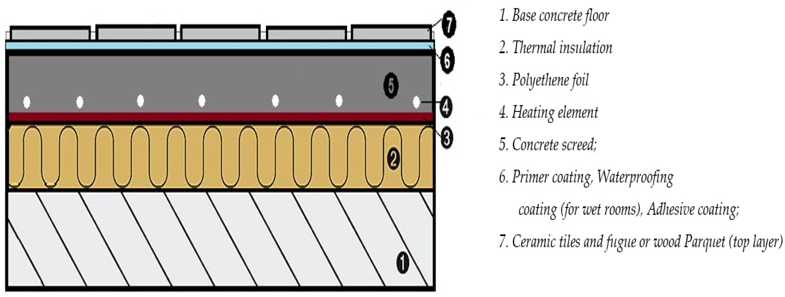
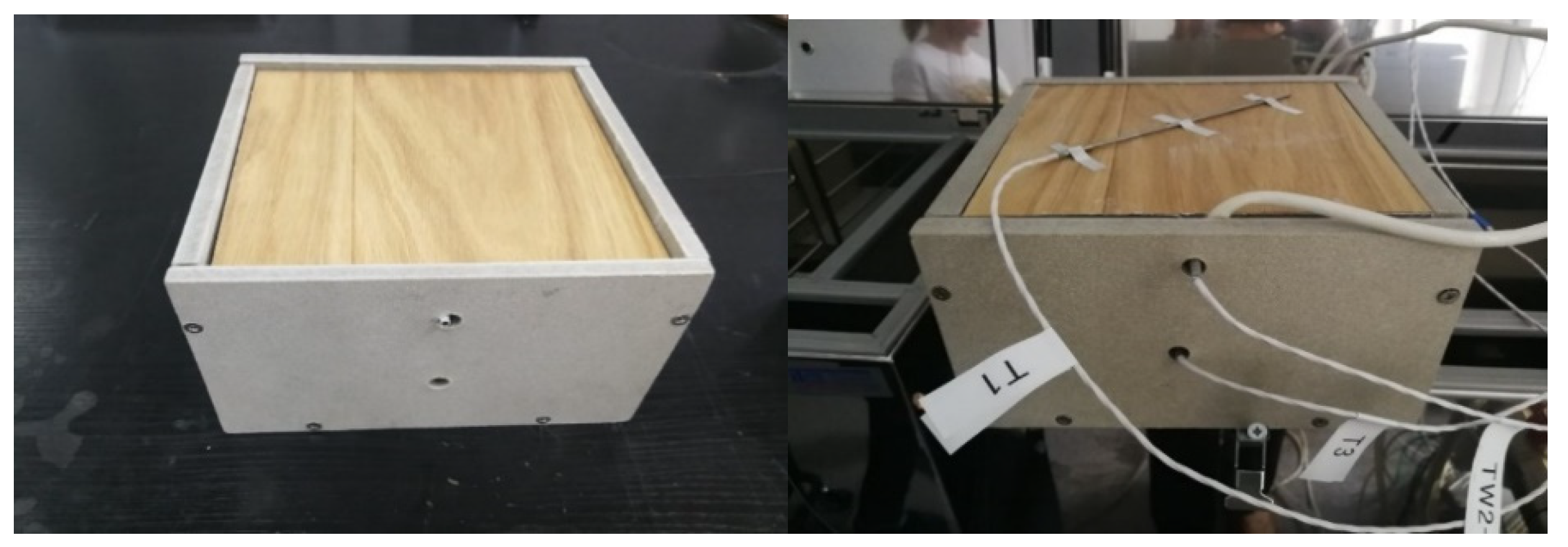
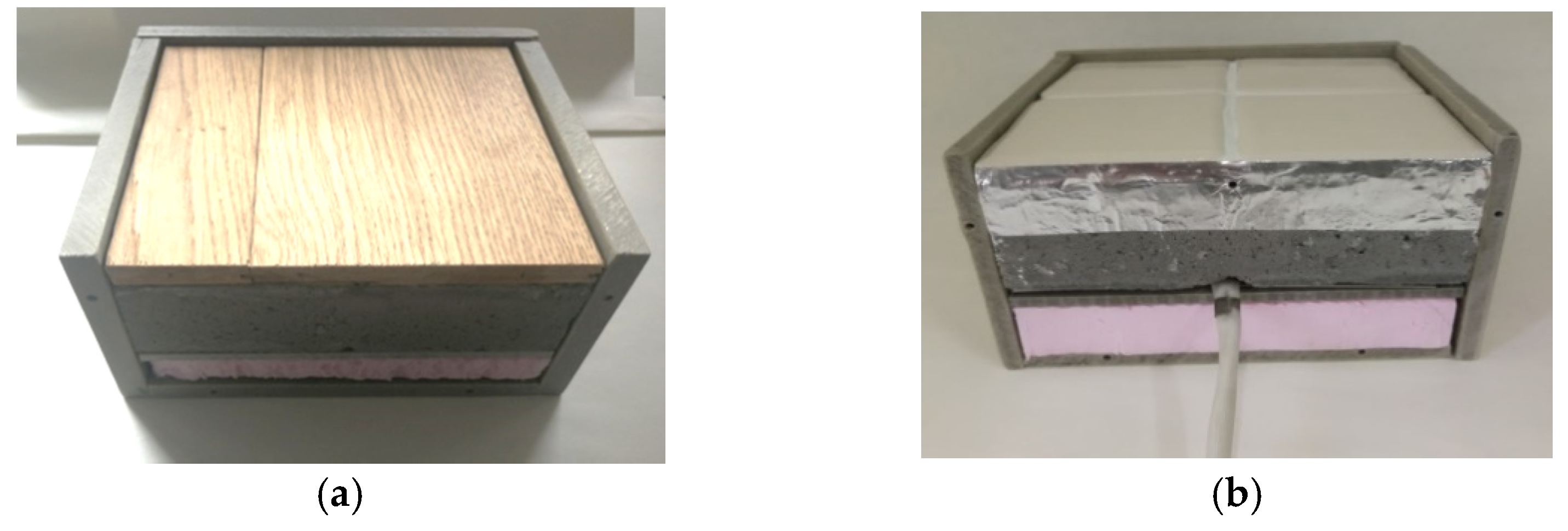
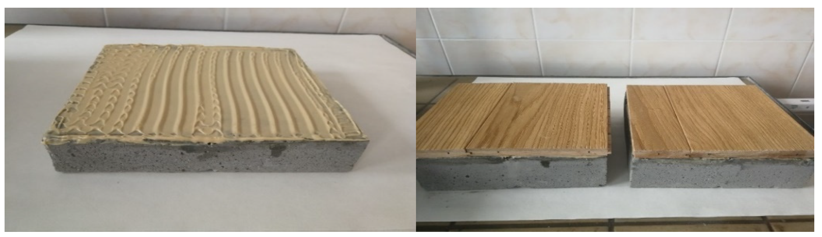
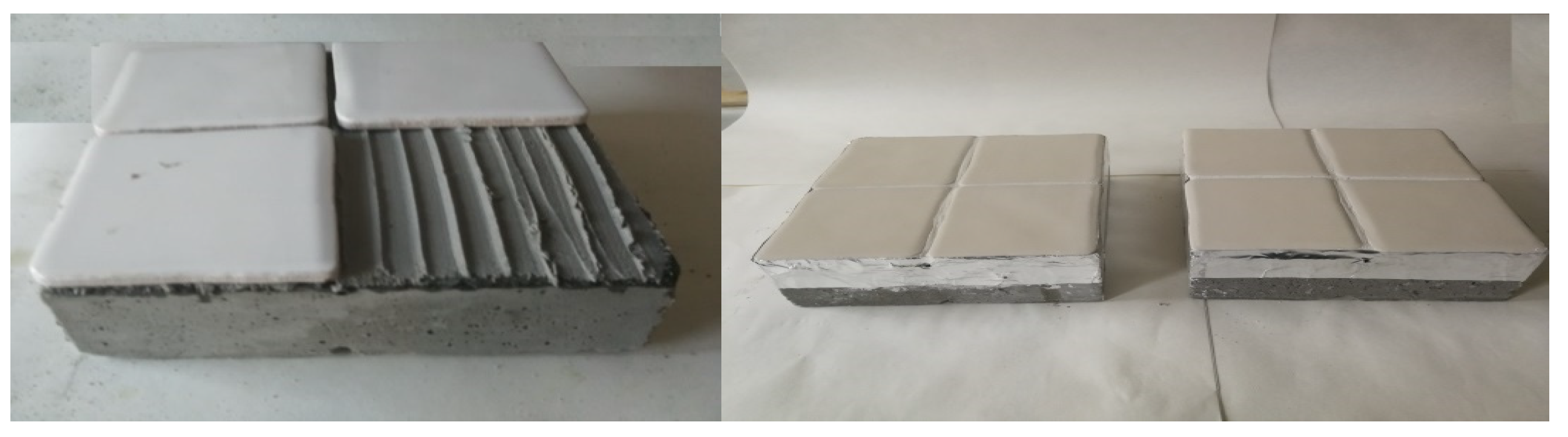
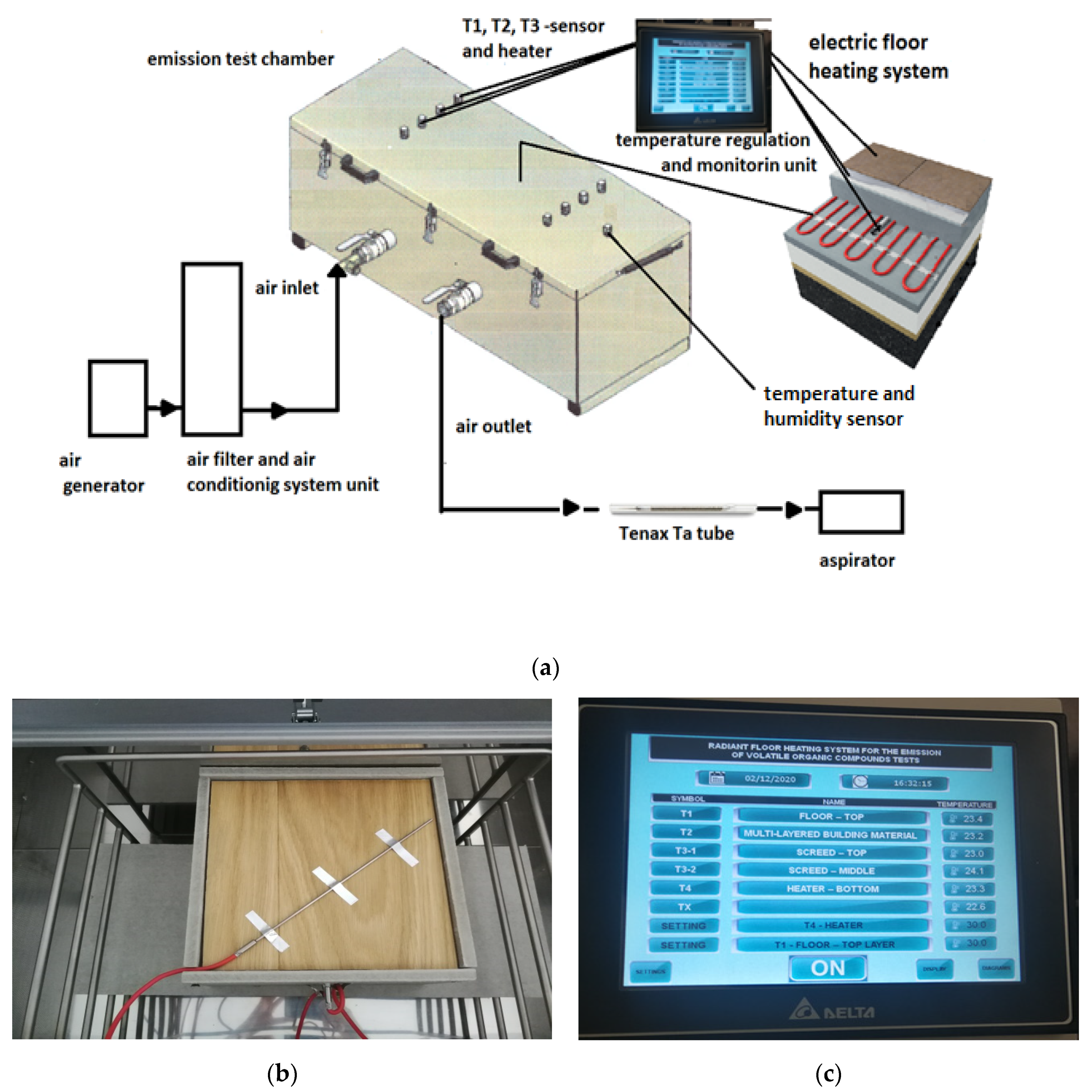
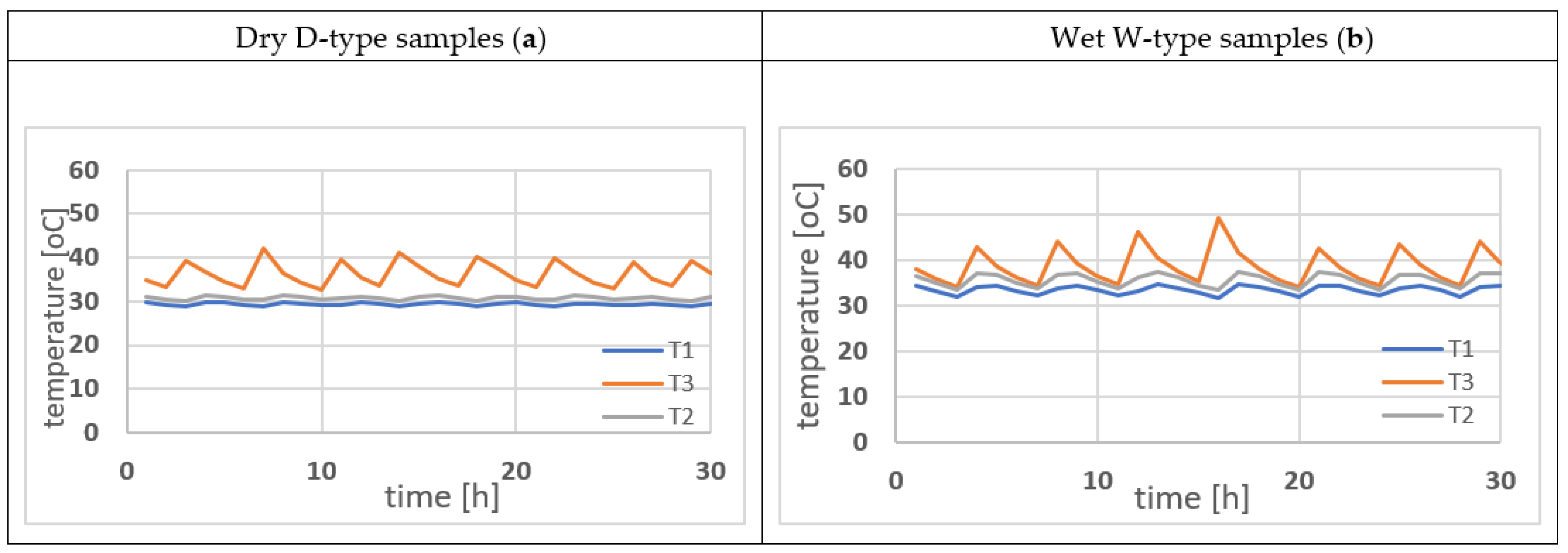
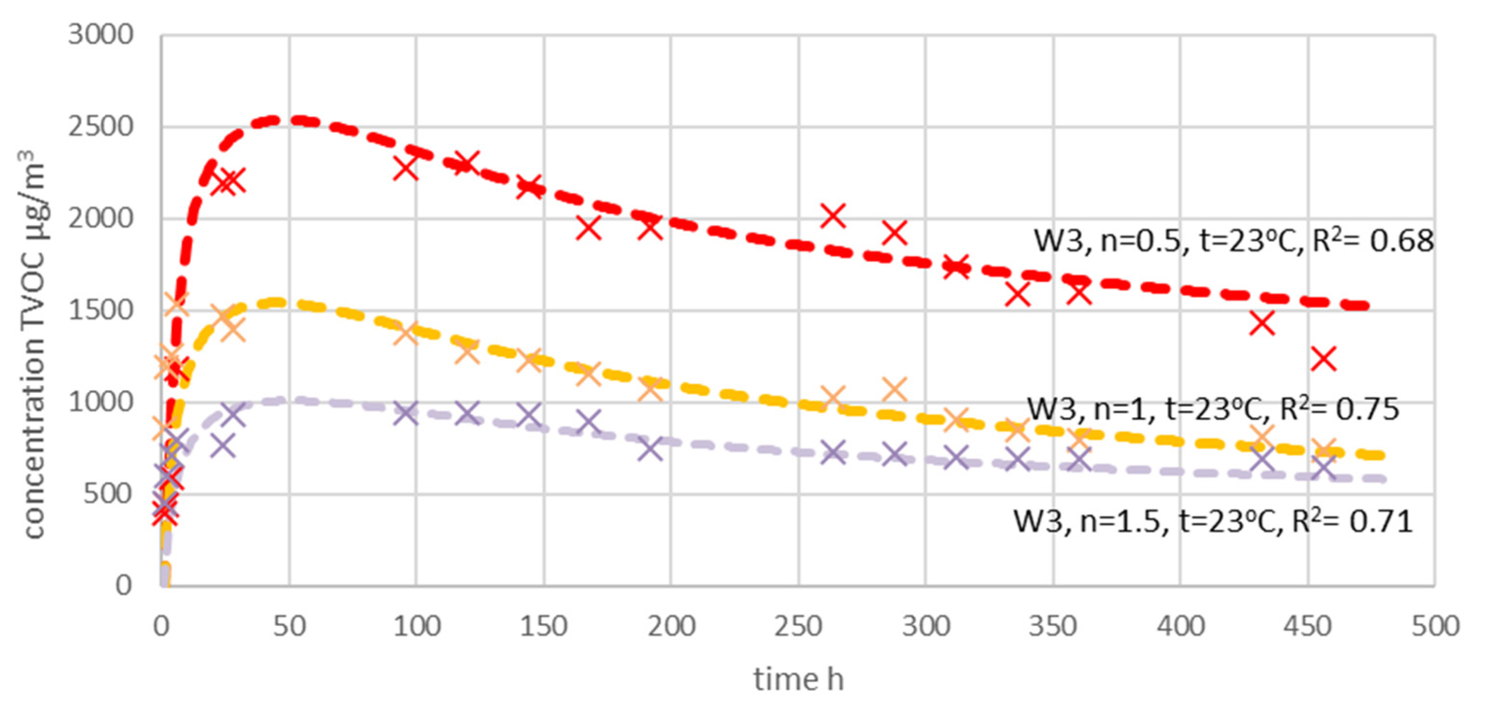
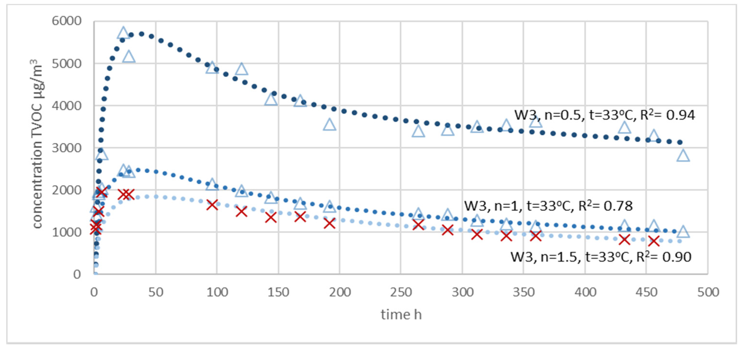
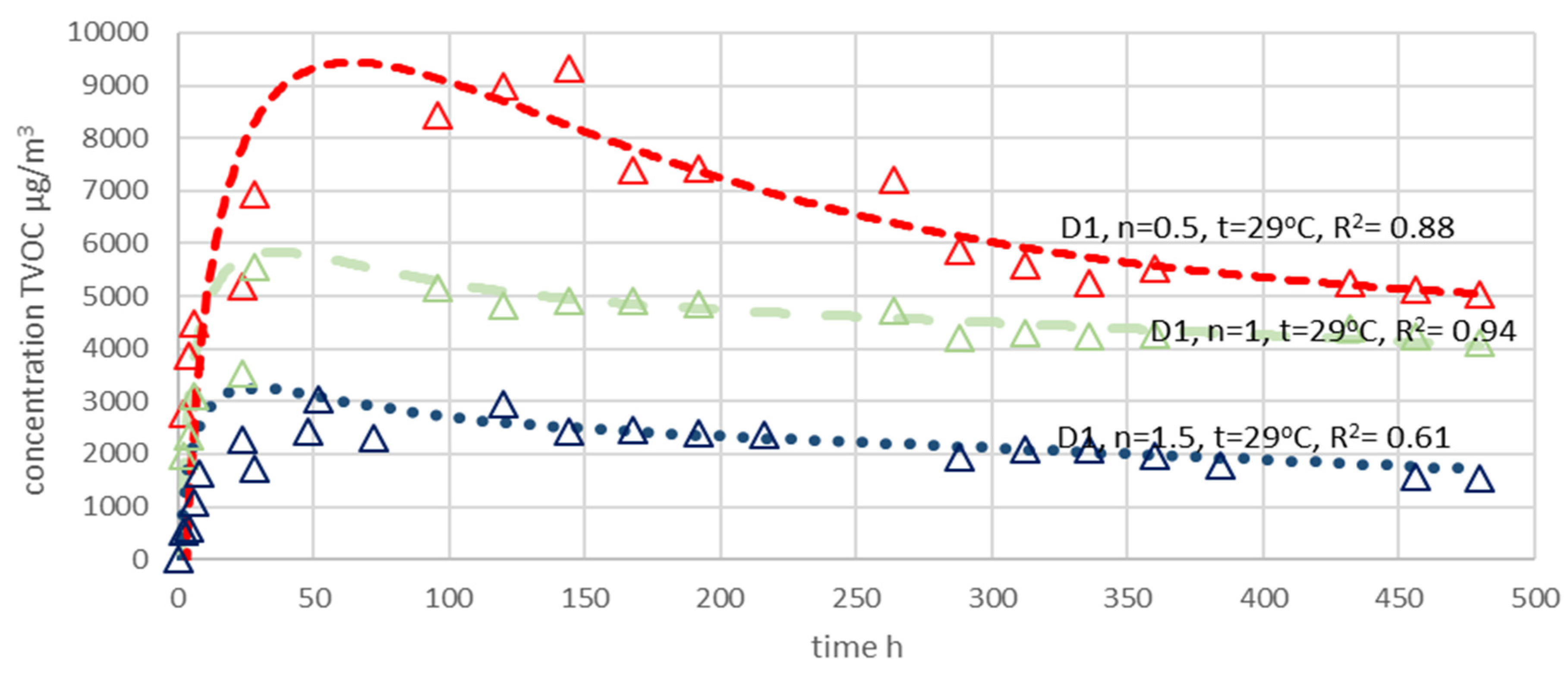
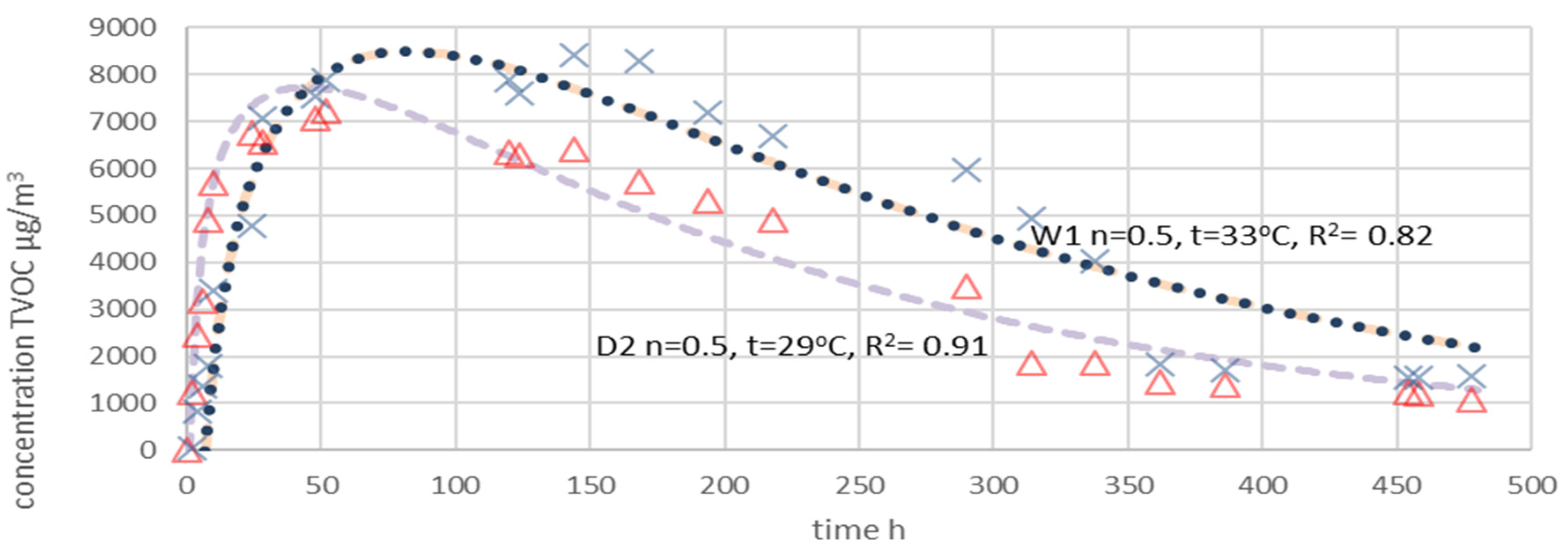
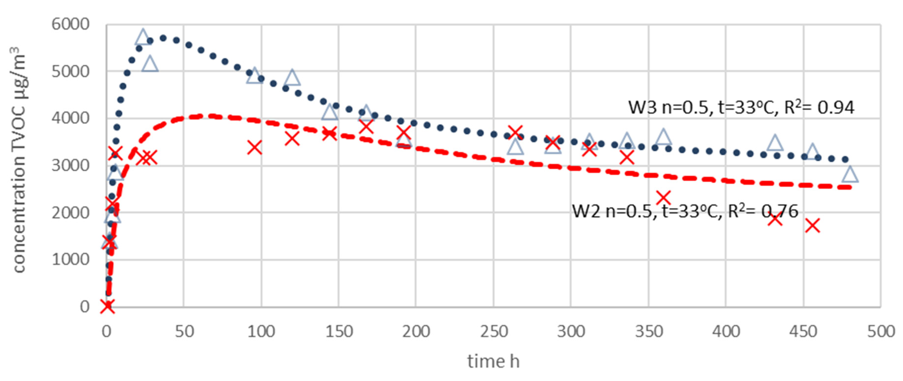
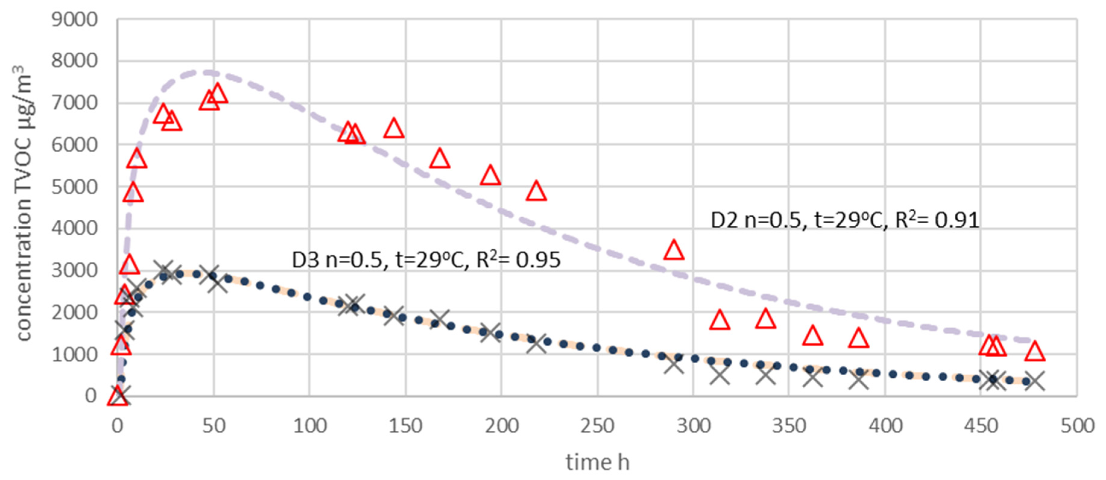
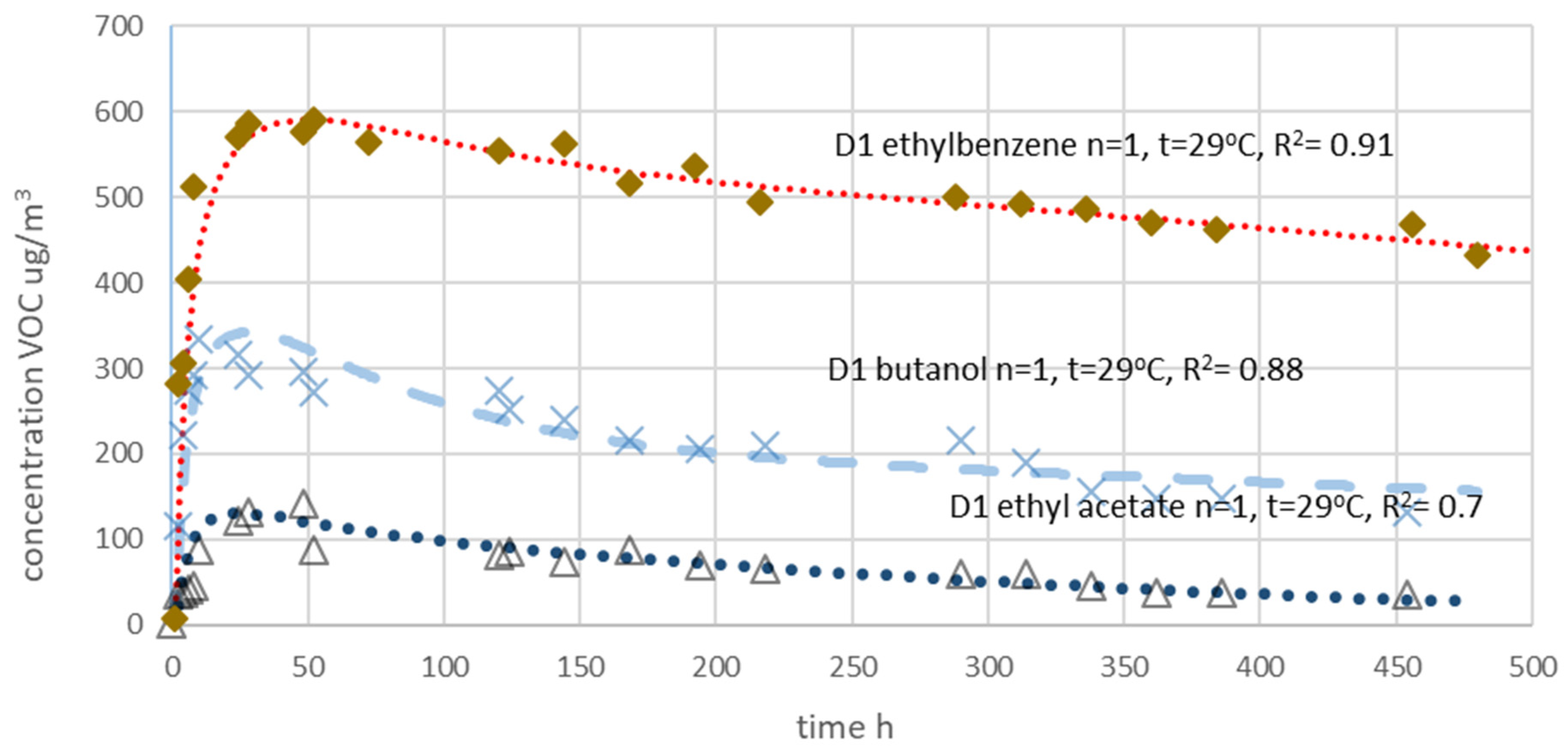
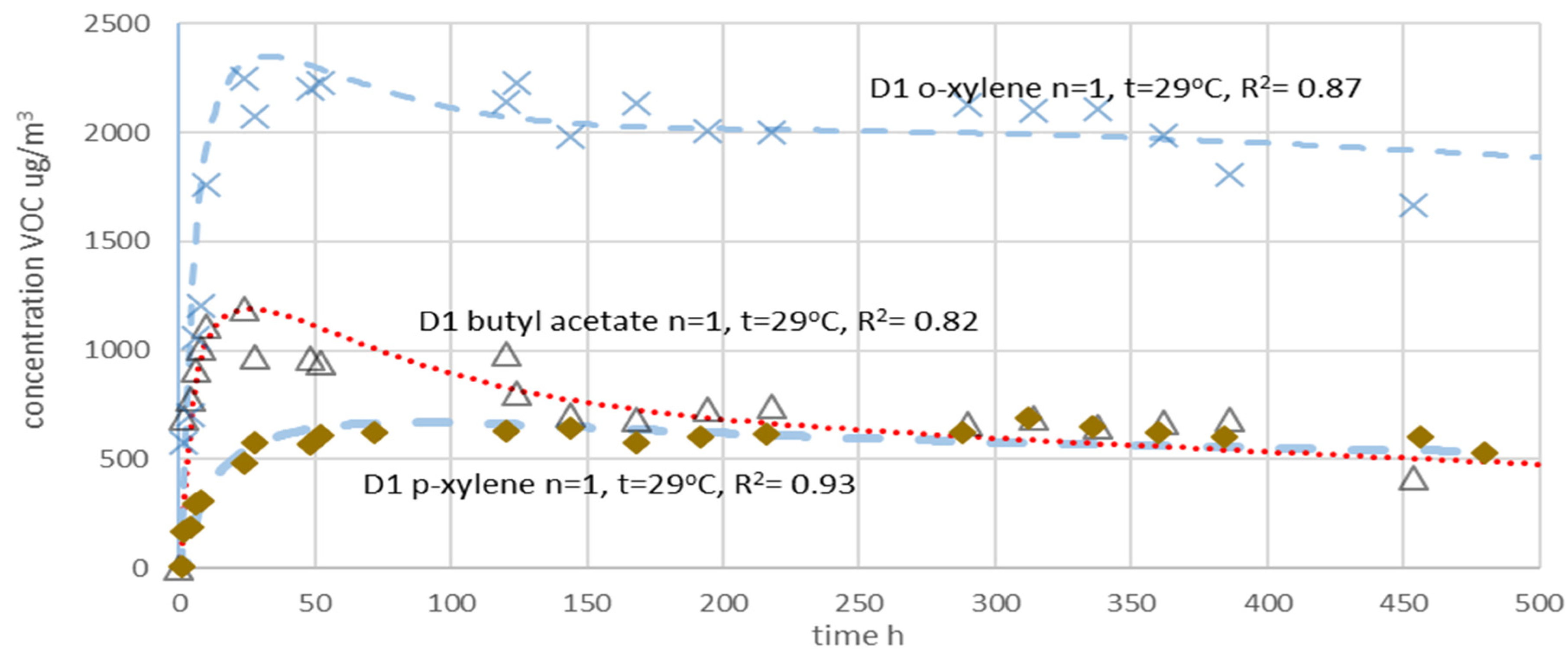
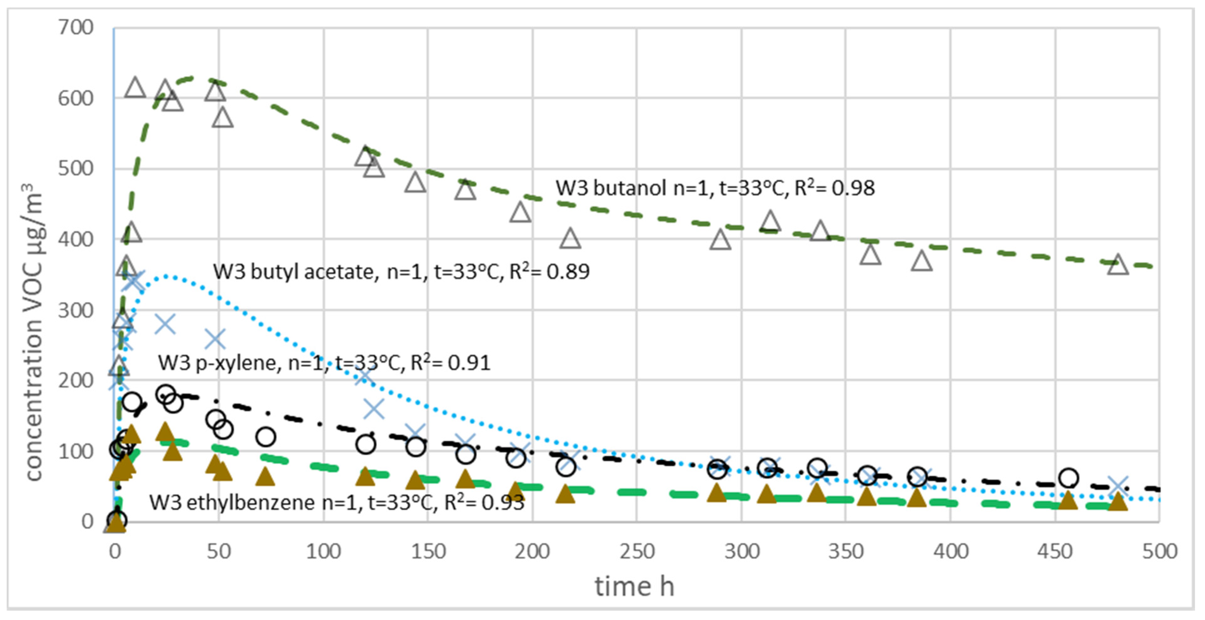
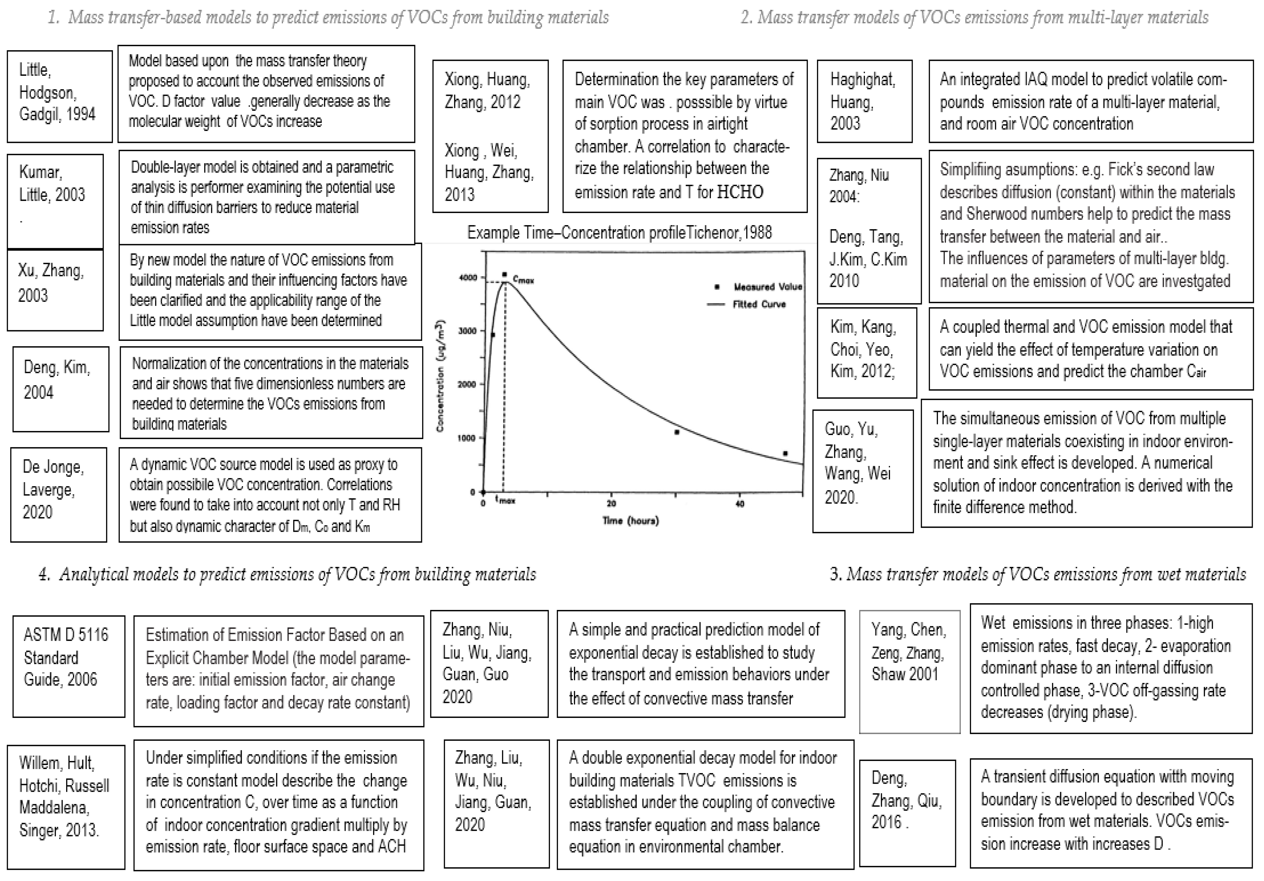
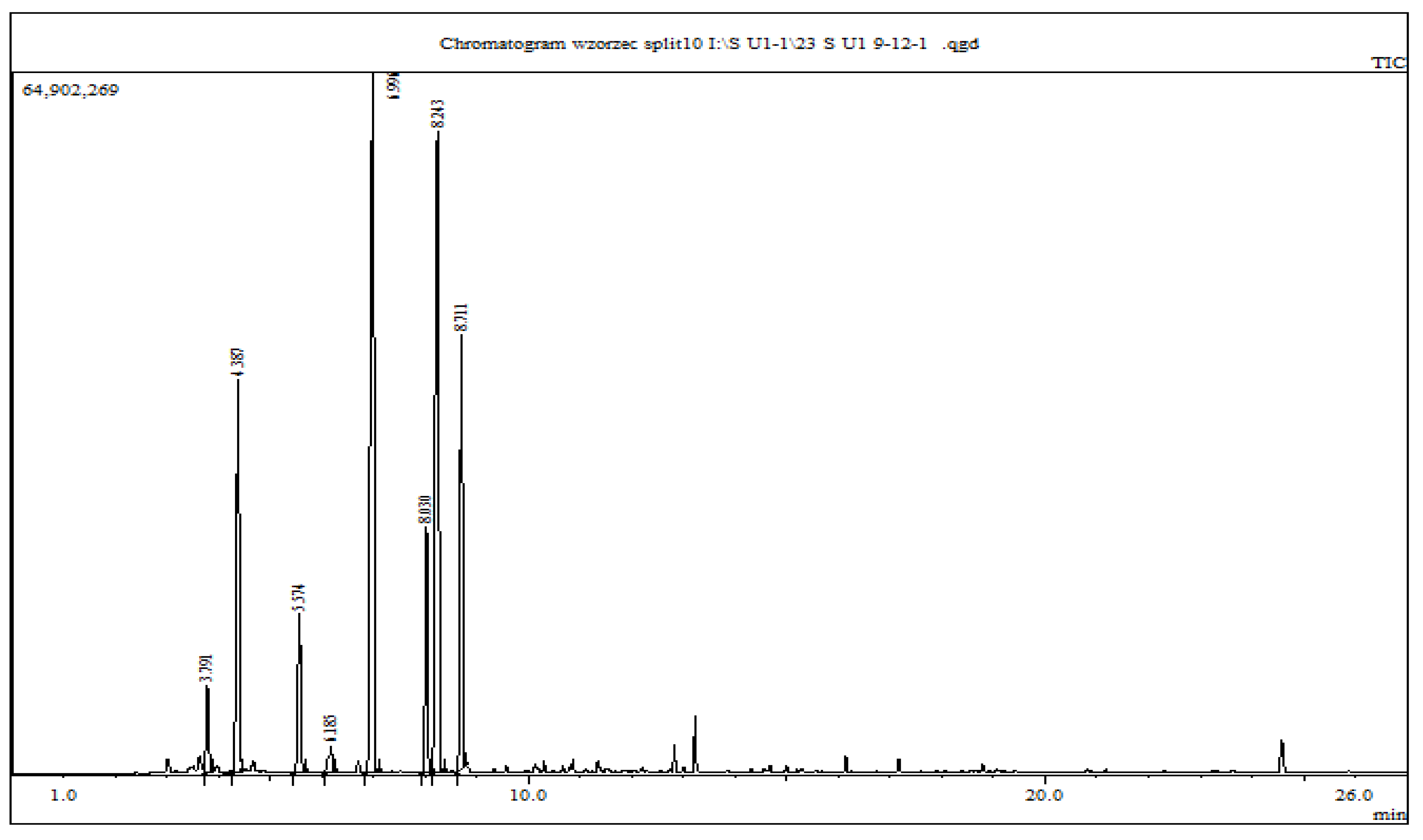
Table 1.
Main chemical composition of products located under the top of the heating floor.
| Type of Product | Main Chemical Compounds | No. of Components | Abbreviations |
|---|---|---|---|
| Primer | P | ||
| Polyurethane solvent primer | butanol, butyl acetate, ethylbenzene, xylene (isomers) | 1 | P-PS1 |
| Base on water dispersion primer | butanol, butyl acetate | 1 | P-D |
| Epoxy primer | ethyl acetate, toluene, 2-butanone, ethanol, benzyl alcohol | 2 | P-E |
| Waterproofing products | W | ||
| Dispersion waterproofing | butyl acetate, xylene (isomers), cyclohexanol, styrene | 1 | W-DM |
| Polymer–cement waterproofing | butanol, xylene isomers, ethylene glycol, benzyl alcohol | 2 | W-FCM-1 |
| Polymer–cement waterproofing | butanol, butyl acetate, butyl ether | 2 | W-FCM-2 |
| Wood floor adhesive | WFA | ||
| Polyurethane adhesive | 2-hexanone,ethyl acetate, butyl acetate, xylene (isomers) | 2 | WFA-P-2C |
| Polyurethane–epoxy adhesive | acetone, 2-butanone, 2-hexanone, methyl acetate, ethyl acetate, toluene ethylbenzene, xylene (isomers) | 2 | WFA-PE |
| Ceramic adhesives | CA | ||
| Polyurethane–epoxy adhesive | acetone, 2-butanone, 2-hexanone, methyl acetate, ethyl acetate, toluene ethylbenzene, xylene (isomers), limonene, ethanol | 2 | KP-PE |
| Epoxy adhesive | ethanol butanol ethyl acetate, butyl acetate, toluene | 2 | KC-E |
Table 2.
Sets of multilayer construction products—D type (top layer is wooden oak parquet).
| Product | D1 | D2 | D3 |
|---|---|---|---|
| Primer | Polyurethane solvent primer | Polyurethane solvent primer | Based on water dispersion primer |
| Wood floor adhesive | Polyurethane adhesive | Polyurethane–epoxy adhesive | Polyurethane–epoxy adhesive |
Table 3.
Sets of multilayer construction products—W type (top layer is a ceramic tile).
| Product | W1 | W2 | W3 |
|---|---|---|---|
| Primer | Polyurethane solvent primer | Epoxyprimer | Polyurethanesolventprimer |
| Waterproofing products | Dispersion waterproofing | Polymer–cement waterproofing (1) | Polymer–cement waterproofing (2) |
| Ceramic adhesive | Polyurethane–epoxyadhesive | Epoxy adhesive | Epoxy adhesive |
Table 4.
Test parameters fixed values and accuracy of measurement.
| Type | Chamber with Heating No.1 | Chamber without Heating No.2 | |||||
|---|---|---|---|---|---|---|---|
| Top Layer | Heater | Multilayer Coating | RH | T1/T2 | RH | Tchamber | |
| T1 (°C) | T3 (°C) | T2 (°C) | (%) | (°C) | (%) | (°C) | |
| D | 29±0.5 | 36 ± 0.5 | 31 ± 0.5 | 50 ± 2 | 23 ± 0.5 | 50 ± 2 | 23 ± 1 |
| W | 33 ± 0.5 | 38± 0.5 | 35 ± 0.5 | 80 ± 2 | 23 ± 0.5 | 80 ± 2 | 23 ± 1 |
Table 5.
Increase inTVOC concentration ΔCmax (µg m−3) caused by an increase or decrease of parameters T1 and n.
Table 5.
Increase inTVOC concentration ΔCmax (µg m−3) caused by an increase or decrease of parameters T1 and n.
| An Increase in the Maximum Chamber Concentration ΔCmax due to an Increase in the Emission Surface Temperature ΔT1 from 23 °C to 33 °C Air Changes n = 1.0 h−1 | An Increase in the Maximum Chamber Concentration ΔCmax due to a Decrease in Ventilation Efficiency at a Constant Temperature 23 °C, by Reducing the Number of Air Changes from 1.0 h−1 to 0.5 h−1 | An Increase in the Maximum Chamber Concentration ΔCmax due to a Decrease in Ventilation Efficiency at a Constant Temperature 33 °C, (or 29 °C) by Reducing the Number of Air Changes from 1.0 h−1 to 0.5 h−1 | |||||||
|---|---|---|---|---|---|---|---|---|---|
| W3 (RH 80%) | 23 °C | 33 °C | ΔT1 → ΔCmax | n = 1.0 h−1 → | 0.5 h−1 | ΔCmax | n = 1.0 h−1 → | 0.5 h−1 | ΔCmax |
| W3 → Cmax | 2550 | 5700 | 3150 | 1500 | 2500 | 1000 | 2500 | 5700 | 3200 |
| % ΔCmax = +124% | % ΔCmax = +67% | % ΔCmax = +128% | |||||||
| D1 (RH 50%) | 23 °C | 29 °C | ΔT1 → ΔCmax | n = 1.0 h−1 → | 0.5 h−1 | ΔCmax | n = 1.0 h−1 → | 0.5 h−1 | ΔCmax |
| D1 → Cmax | 3300 | 9350 | 6050 | 2600 | 3500 | 900 | 5900 | 9350 | 3100 |
| % ΔCmax = +183% | % ΔCmax = +35% | % ΔCmax = +53% | |||||||
Table 6.
Increase of TVOC concentration Cmax and C480 (µg m−3) caused by a change in the multilayer sample structure oftype D or W to the chemical composition of one layer: a primer (air exchange n = 0.5).
Table 6.
Increase of TVOC concentration Cmax and C480 (µg m−3) caused by a change in the multilayer sample structure oftype D or W to the chemical composition of one layer: a primer (air exchange n = 0.5).
| Sample | CmaxValues from the Emission Profiles | C480 hValues from the Emission Profiles | ||
|---|---|---|---|---|
| with G-PR1 | without G-PR1 | with G-PR1 | without G-PR1 | |
| W3 | ~5700 | ~3100 | ||
| W2 | ~4000 | ~2600 | ||
| D2 | ~7800 | ~1300 | ||
| D3 | ~2900 | ~40 | ||
Table 7.
Main VOC compounds with the highest concentration detected by GC-MS (D-type samples).
| D1 | D2 | D3 | |
|---|---|---|---|
| Ketones | acetone | acetone | |
| 2-butanon | 2-butanon | ||
| 2-hexanone | 2-hexanone | 2-hexanone | |
| Alcohols | butanol | Butanol | butanol |
| ethyl acetate | methyl acetate | methyl acetate | |
| Esters | ethyl acetate | ethyl acetate | |
| butyl acetate | butyl acetate | butyl acetate | |
| toluene | toluene | ||
| Hydrocarbons | ethylbenzene | ethylbenzene | ethylbenzene |
| aromatic | o-xylene | o-xylene | o-xylene |
| m-p-xylene | m-p-xylene | m-p-xylene |
Table 8.
Main VOC compounds with the highest concentration detected by GCMS (W1–W3).
| W1 | W2 | W3 | |
|---|---|---|---|
| Ketones | acetone | ||
| 2-butanone | |||
| 2-hexanone | |||
| Alcohols | ethanol | ethanol | |
| butanol | butanol | butanol | |
| methyl acetate | |||
| Esters | ethyl acetate | ||
| butyl acetate | butyl acetate | butyl acetate | |
| toluene | Toluene | Toluene | |
| Hydrocarbons aromatic | ethylbenzene | ethylbenzene | |
| xylene | o-xylene | ||
| xylene | m-p-xylene | ||
| Rest | limonene | limonene | |
| 2-butanol |
Table 9.
Comparing the Cmax (µg/m3) and C480 h observed from the emission profiles of the four selected VOCs emitted from samples D1 tested in t = 29 °C and samples W3 tested in t = 33 °C (ACH n = 1.0 h−1).
Table 9.
Comparing the Cmax (µg/m3) and C480 h observed from the emission profiles of the four selected VOCs emitted from samples D1 tested in t = 29 °C and samples W3 tested in t = 33 °C (ACH n = 1.0 h−1).
| Sample | 1-Butanol | Ethylbenzene | Butyl Acetate | m-p-Xylene |
|---|---|---|---|---|
| Cmax values from the emission profiles | ||||
| D1 | 340 | 600 | 1200 | 700 |
| W3 | 630 | 110 | 340 | 180 |
| C480 h values from the emission profiles | ||||
| D1 | 160 | 450 | 400 | 450 |
| W3 | 380 | 30 | 40 | 60 |
Table 10.
Illustrative values of the X coefficient of the C(t) model (17) as a function of time and the number of layers of the heated floor system.
Table 10.
Illustrative values of the X coefficient of the C(t) model (17) as a function of time and the number of layers of the heated floor system.
| a = 1 For | a = 0.7 For | a = 0.6 For | a = 0.5 For | |
|---|---|---|---|---|
| Time of Test t(h) | 1 Layer | 2 Layers | 3 Layers | 4 Layers |
| X = a·log(t) | ||||
| 1 | 0 | 0 | 0 | 0 |
| 2 | 0.3 | 0.21 | 0.18 | 0.15 |
| 3 | 0.47 | 0.33 | 0.29 | 0.24 |
| 4 | 0.6 | 0.42 | 0.36 | 0.3 |
| 5 | 0.69 | 0.49 | 0.42 | 0.35 |
| 6 | 0.77 | 0.54 | 0.47 | 0.39 |
| 7 | 0.84 | 0.59 | 0.51 | 0.42 |
| 8 | 0.89 | 0.63 | 0.54 | 0.45 |
| 9 | 0.94 | 0.67 | 0.57 | 0.48 |
| 10 | 1 | 0.7 | 0.6 | 0.5 |
| 16 | 0.84 | 0.72 | 0.6 | |
| 24 | 0.97 | 0.83 | 0.69 | |
| 32 | 1 | 0.9 | 0.75 | |
| 40 | 0.96 | 0.8 | ||
| 48 | 1 | 0.84 | ||
| 64 | 0.9 | |||
| 80 | 0.95 | |||
| 96 | 1 | |||
Table 11.
Determined coefficients k1 and k2 of the equation C(t) (17) (TVOC) for each tested dry floor system D1–D3 (29 °C, RH = 50%) and wet W1–W3 (33 °C and RH = 80%) in the range of ACH n = 0.5–1.5 h−1.
Table 11.
Determined coefficients k1 and k2 of the equation C(t) (17) (TVOC) for each tested dry floor system D1–D3 (29 °C, RH = 50%) and wet W1–W3 (33 °C and RH = 80%) in the range of ACH n = 0.5–1.5 h−1.
| Value of Parameter k1 | Value of Parameter k2 | |||
|---|---|---|---|---|
| Tested | ||||
| Sample | Min | Max | Min | Max |
| D1 | 0.007 | 0.02 | 0.001 | 0.002 |
| D2 | 0.007 | 0.01 | 0.002 | 0.003 |
| D3 | 0.006 | 0.02 | 0.001 | 0.002 |
| W1 | 0.004 | 0.01 | 0.0005 | 0.001 |
| W2 | 0.007 | 0.01 | 0.0005 | 0.001 |
| W3 | 0.01 | 0.02 | 0.001 | 0.002 |
Table 12.
Influence of changes in k1 and k2 parameters of model Equation (17) on the coefficient of fitting the model to experimental points.
Table 12.
Influence of changes in k1 and k2 parameters of model Equation (17) on the coefficient of fitting the model to experimental points.
| Analysed Parameter of C(t) | Changing a Parameter by a Value of | R2 Coefficient Change |
|---|---|---|
| k1 | ±5% | −0.2% |
| ±10% | −0.5% | |
| ±30% | −1.6% | |
| ±50% | −3.0% | |
| ±100% | −7.0% | |
| k2 | ±5% | −0.5% |
| ±10% | −0.9% | |
| ±30% | −3.0% | |
| ±50% | −6.0% | |
| ±100% | −14.0% |
Table 13.
Comparing the C480 h (µg/m3) observed from the emission profiles by the model (17) and experimental values of four selected VOCs emitted from samples D1 tested in t = 29 °C and samples W3 tested in t = 33 °C (ACH n = 1.0 h−1).
Table 13.
Comparing the C480 h (µg/m3) observed from the emission profiles by the model (17) and experimental values of four selected VOCs emitted from samples D1 tested in t = 29 °C and samples W3 tested in t = 33 °C (ACH n = 1.0 h−1).
| Sample | 1-Butanol | Ethylbenzene | Butyl Acetate | m-p-Xylene | ||||
|---|---|---|---|---|---|---|---|---|
| Model | Exp. | Model | Exp. | Model | Exp. | Model | Exp. | |
| D1 | 160 | 133 | 450 | 337 | 400 | 416 | 450 | 477 |
| W3 | 380 | 380 | 30 | 35 | 40 | 66 | 60 | 66 |
Publisher’s Note: MDPI stays neutral with regard to jurisdictional claims in published maps and institutional affiliations. |
© 2021 by the authors. Licensee MDPI, Basel, Switzerland. This article is an open access article distributed under the terms and conditions of the Creative Commons Attribution (CC BY) license (https://creativecommons.org/licenses/by/4.0/).
Share and Cite
MDPI and ACS Style
Piasecki, M.; Kostyrko, K.B.; Goljan, A. The Ability to Control VOC Emissions from Multilayer Building Materials. Appl. Sci. 2021, 11, 4806. https://0-doi-org.brum.beds.ac.uk/10.3390/app11114806
AMA Style
Piasecki M, Kostyrko KB, Goljan A. The Ability to Control VOC Emissions from Multilayer Building Materials. Applied Sciences. 2021; 11(11):4806. https://0-doi-org.brum.beds.ac.uk/10.3390/app11114806
Chicago/Turabian StylePiasecki, Michał, Krystyna Barbara Kostyrko, and Anna Goljan. 2021. "The Ability to Control VOC Emissions from Multilayer Building Materials" Applied Sciences 11, no. 11: 4806. https://0-doi-org.brum.beds.ac.uk/10.3390/app11114806
Note that from the first issue of 2016, this journal uses article numbers instead of page numbers. See further details here.