Thermal Inertia Characterization of Multilayer Lightweight Walls: Numerical Analysis and Experimental Validation

Abstract

The thermal inertia properties of construction elements have gained a great deal of importance in building design over the last few years. Many investigations have shown that this is the key factor to improve energy efficiency and obtain optimal comfort conditions in buildings. However, experimental tests are expensive and time consuming and the development of new products requires shorter analysis times. In this sense, the goal of this research is to analyze the thermal behavior of a wall made up of lightweight concrete blocks covered with layers of insulating materials in steady- and transient-state conditions. For this, numerical and experimental studies were done, taking outdoor temperature and relative humidity as a function of time into account. Furthermore, multi-criteria optimization based on the design of the experimental methodology is used to minimize errors in thermal material properties and to understand the main parameters that influence the numerical simulation of thermal inertia. Numerical Finite Element Models (FEM) will take conduction, convection and radiation phenomena in the recesses of lightweight concrete blocks into account, as well as the film conditions established in the UNE-EN ISO 6946 standard. Finally, the numerical ISO-13786 standard and the experimental results are compared in terms of wall thermal transmittance, thermal flux, and temperature evolution, as well as the dynamic thermal inertia parameters, showing a good agreement in some cases, allowing builders, architects, and engineers to develop new construction elements in a short time with the new proposed methodology.

1. Introduction

Thermal comfort is one of the most valued concepts in the habitability of both residential and office buildings. Energy consumption is needed to achieve adequate thermal comfort, and the large energy demands of buildings have significant environmental impacts. Therefore, buildings must be designed to minimize heat loss through their enclosures and to reduce energy demands [1].

Increasing the thermal resistance (R, m²K/W) of building enclosures is a well-known method to reduce heat loss. Thermal transmittance (U-value, W/m²K) is the inverse of the total resistance values of enclosure heat transfer (R_tot). The U-value is the rate of heat transfer (in watts) through 1 m² of a building element and is determined by the difference in temperature across the wall. Most building standards [2] evaluate the U-value of the materials that form the enclosure, characterizing their steady-state thermal physical properties. However, this method has the disadvantage of not accounting for the heat storage capacity of materials when environmental conditions change. In recent years, it has been concluded that it is not possible to design thermally efficient buildings based on U-value alone. The determination of the transient thermal behavior of different construction solutions is receiving a great deal of interest in order to advance the concept of the thermal inertia of construction elements [3].

Thermal inertia is the ability of a material to maintain the thermal energy it has been exposed to and to progressively release heat. Thermal inertia reduces the need to supply heated or cooled air, thus saving energy. Values of thermal inertia must be analyzed under real conditions of temperature and humidity, which vary over time. In addition, they must take the thermal storage capacity of each of the layers that constitute the constructive element to be analyzed into account. Using thermal inertia values, it will be possible to obtain more accurate values of thermal comfort than when using thermal transmittance alone. Previous studies on thermal inertia in Northern Italy showed that the difference in heating demands between low and high thermal inertia walls was about 10%. When considering cooling demands, the difference increased to 20% [4]. Kossecka and Kosny [5] stated that the difference in energy requirements between walls with different thermal efficiencies ranged between 2.3% and 11.3%, depending on the climate, with the difference being more pronounced in the case of an increased solar exposure and diurnal temperature differences. Asan and Sancaktar [6] studied the influence of time lag and decrement factor on materials’ thermophysical properties, accounting for material thickness and its position in the wall. In addition, Asan [7] also studied the effect of wall insulation thickness and position on the time lag and decrement factor, and determined the optimum insulation position to achieve the minimum decrement factor and maximum time lag. Ozel and Pithtili [8] also established the optimum insulation location and its distribution in walls to improve thermal inertia. In a study by Di Perna et al. [9], the influence of thermal mass placed on the inner side of a building envelope was assessed. Simultaneous monitoring was carried out on rooms with high internal heat loads (school classrooms), and the internal inertia of the envelope was varied using an insulating panel on the interior side. Ng et al. [10] studied the most influential parameters in thermal inertia on lightweight concrete wall panels, and found that thermal diffusivity had a positive relationship with the thermal inertia of wall panels. Based on a 1D numerical model, Jin et al. [11] studied the influence of heat flux on time lag and the decrement factor on the thermal properties and thickness of walls. They also reported the decrement factor for several building materials. Kontoleon et al. [12] analyzed the impact of heat flux, concrete density, and conductivity on the decrement factor and time lag, and obtained the optimal decrement factor and time lag values for concretes with 950 kg/m³ in wall assemblies with one layer of insulation. They also found that the placement of insulation into two layers improves the optimal decrement factor and time lag values using concretes with a density above 1200 kg/m³. The best results were obtained by placing the insulation on the external surface and the center of the enclosure.

With respect to the heat transfer numerical simulation of concrete walls with cavities, del Coz et al. [13,14] and Gencel et al. [15] focused on the evaluation of thermal transmittance properties and the optimization of construction elements under steady-state thermal conditions. These studies highlighted the importance of the size of holes and their distribution, and of radiation and convection phenomena in cavities. A study by Arendt et al. [16] complemented these studies by taking into account dynamic thermal parameters, such as the decrement factor, time lag, and thermal conductivity. They used numerical and analytical models to determine that the optimal percentage of cavities to achieve ideal comfort conditions was between 45% and 65% with respect to the material volume. In contrast, thermal conductivity decreases proportionally with increased cavity volume. Zhang et al. [17] concluded that the transient thermal performance of walls is optimal for thermal conductivity values lower than 1.0 W/mK. Their study was based on a reduction in material conductivity values using both block and hole filling, increasing the total thickness of the block and the number of cavities in parallel. Soret et al. [18] proposed a numerical method to obtain the thermal inertia of a building’s components using its thermal insulation parameters in order to predict fire reaction behavior.

It is critical that the following factors be identified to obtain the thermal inertia properties of construction elements: layer distribution; thermo-physical characteristics of the materials used; temperature evolution; and the difference between indoor and outdoor thermal conditions.

In general, according to the existing literature mentioned above, high time lags and low decrement factor values are preferred to obtain optimal comfort conditions inside buildings. It can be concluded that interior thermal comfort conditions could vary significantly for envelopes with the same thermal resistances but with different densities.

The objective of this study was to analyze the thermal behavior under steady- and transient-state conditions of a wall made up of lightweight concrete blocks covered with layers of insulating materials. 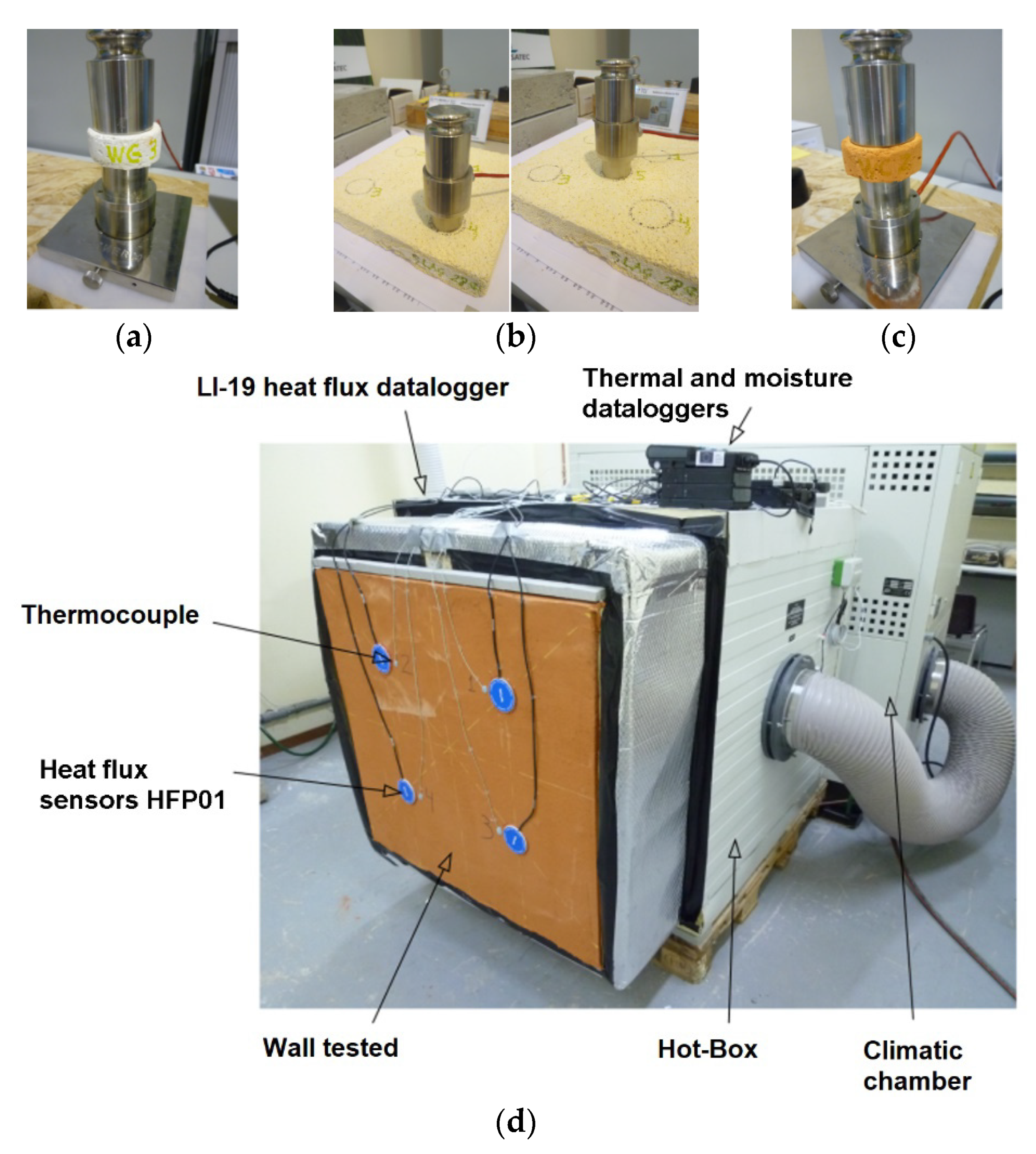The material used in the block manufacturing has been shown to possess thermal and structural advantages, including a longer product life cycle than other construction materials, low structural weight, excellent behavior at high temperatures, and good thermal insulation values due to its low thermal conductivity [19,20]. 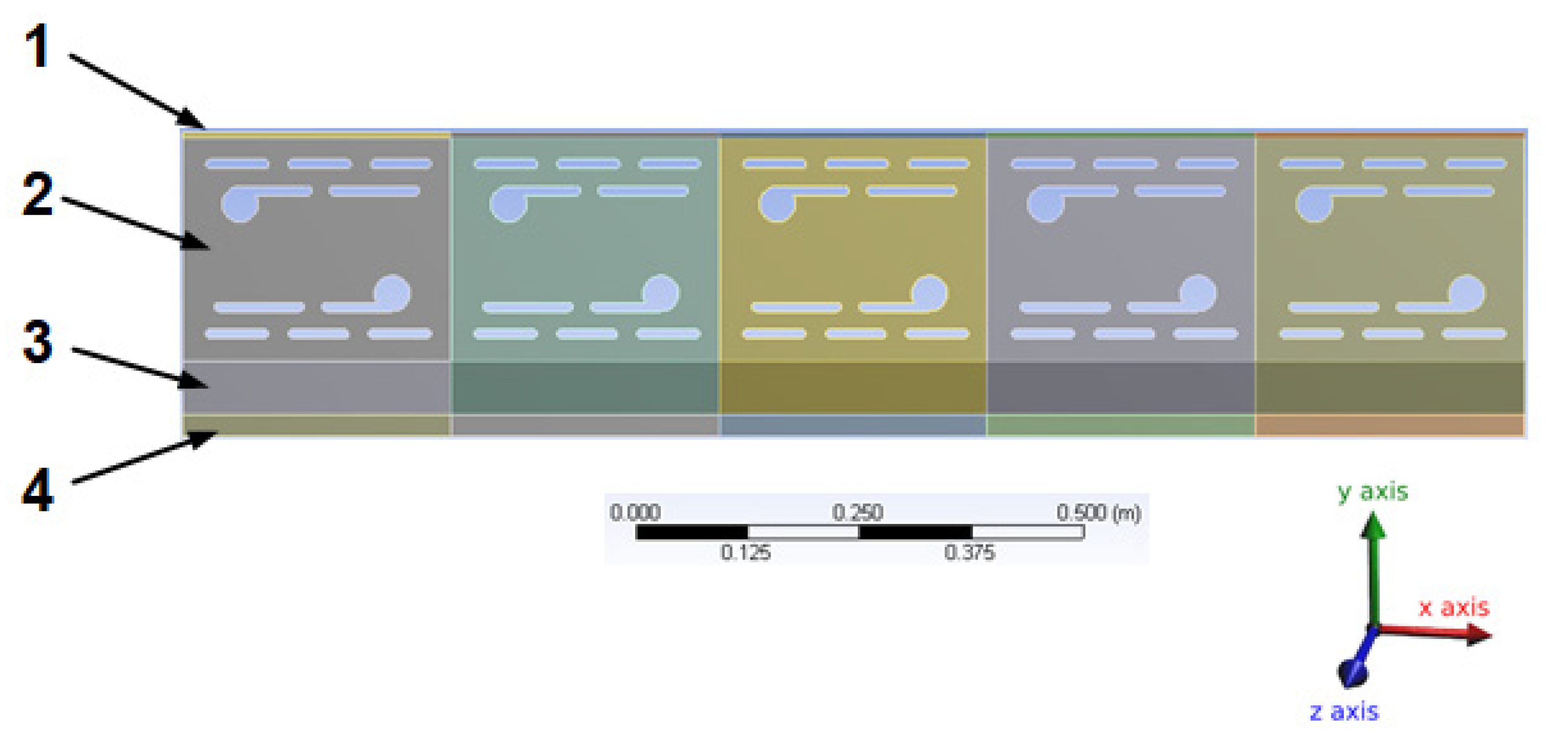In this study, experimental tests were performed in a 1 m² instrumented hot-box climatic chamber, and the material was subjected to variable temperature and humidity conditions to obtain thermal inertia values according to the ISO standard rule [3]. We then created a finite element numerical model of a bi-dimensional wall section with holes, which was subjected to the temperature conditions established in the experimental test, both under steady- and transient-state conditions. We then compared the numerical and experimental findings and related them to standard thermal inertia results.

2. Materials and Methods

2.1. Materials Used

Laboratory tests were carried out on different insulation mortar samples and a 1 m² wall with 0.34 m thickness made up of lightweight concrete blocks that were 0.30 m long, 0.25 m thick, and 0.15 m high. The block wall was coated with insulating mortar with a thickness of 0.015 m and 0.060 m. The wall layer composition is shown in

Table 1. Summary of wall materials’ thickness and position.

Material	Layer ID	Acronym	Thickness (m)	Wall Section
Gypsum-Weber grueso ®	1	GWG	0.015
Lightweight brick Airblock 25 ®	2	LWBA25	0.250
Lightweight mortar-Aislone ®	3	LWMA	0.060
Gypsum-Weber pral clima ®	4	GWP	0.015

.

2.2. Experimental Tests

TCI C-Therm equipment was used to assess the thermal properties of the materials used. This was based on the modified transient plane source (MTPS) technique following ASTM D7984-16 [21]. Thermal conductivity and thermal effusivity were measured using a one-sided heat reflectance sensor that applies a momentary constant heat source to the sample. Both thermal properties were measured directly in a short time (see Figure 1). Three samples of layer 1 (Figure 1a; GWG) and layer 4 (Figure 1; GWP) were tested, and we performed a round robin test for the material of layer 3 (Figure 1b; LWMA). We took five measurements for each sample.

Thermal tests were performed using a 1 m² wall that was built and placed in a climatic air-conditioned system that controlled relative humidity (RH) and temperature conditions. The air-conditioned system was joined to a climatic box (hot-box) with a 1 m³ inside volume, where the desired thermal conditions were provided. The wall tested was built and placed over a steel frame and joined to the hot-box, as shown in Figure 1d. The perimeter of the wall has been thermally insulated with low thermal conductivity foam in order to avoid lateral heat losses. Sensors at different locations were used to measure temperature, relative humidity, and thermal fluxes. Sixteen SHT75 capacitive sensors and one Sensirion EK-H3 datalogger were used to measure the temperature and relative humidity, while four Hukseflux HFP01 sensors and four LI-19 data-loggers were used to measure heat fluxes through the wall. The locations of the sensors are shown in Figure 2.

Steady-state thermal transmittance tests were carried out by maintaining a constant temperature (53 ± 0.5 °C) and varying the humidity conditions from 30% to 70% inside the hot-box. The constant laboratory conditions were a temperature of 23 ± 2.5 °C and a relative humidity of 70 ± 2.0%.

The transient thermal transmittance tests were carried out under constant outdoor conditions of relative humidity of 70% inside the hot-box and 70% outside as well as a variable temperature following a sinusoidal law between 10 and 37 °C with a cycle time of 24 h and a minimum number of 4 complete stabilized cycles. The laboratory indoor conditions were 25 °C ± 2.5 °C and 70% RH constant values. Two test directions were considered (see Figure 2). In Direction 1, as shown Figure 2a, Layer 1 was placed on the inside of the hot-box (outdoor conditions) and Layer 4 was in contact with the outside air of the laboratory (indoor conditions). In Direction 2, as shown Figure 2b, Layer 4 was placed on the inside of the hot-box (outdoor conditions) and Layer 1 was in contact with the outside air of the laboratory (indoor conditions).

2.3. Numerical Models

The thermal behavior of the wall was numerically studied using the finite element method (FEM) using ANSYS Workbench software 2020R1. Conduction, convection and radiation phenomena were taken into account in the numerical study. The material properties used in the numerical models were firstly, experimentally determined and, secondly, analyzed using a multi criteria optimization based on design of experiments methodology.

The FEM model has been used in previous works [22] following the calculation method to verify Annex D of the UNE-EN-1745 Standard Rule [23], with an error less than 2%. Furthermore, the thermal performance of different block walls was analyzed with the same finite elements and similar boundary conditions as in this case, showing differences with respect to the experimental results ranging from 0.3 to 1.7% [22].

Consequently, with respect to the complex heat transfer simulation the numerical model is able to simulate the real multilayer wall behavior as a digital twin. However, moisture transport was approximated by means of multi-criteria optimization based on the design of experiments methodology, as described in this manuscript.

Steady-state analysis was carried out using a constant thermal flux on the external face of the wall. Based on this thermal flux, it was possible to obtain the thermal transmittance of the wall. A transient thermal analysis was performed by including the boundary conditions taken from the experimental tests. This was applied to the external face of the wall to measure the temperature evolution inside the hot-box, and we used 4 stabilized cycles of a 24-h-period sine function. We determined the thermal inertia parameters of the wall using this numerical analysis.

2.3.1. Geometrical Model

The 2D geometrical model we developed is shown in Figure 3. It was composed of five blocks that were made up of four materials. The five blocks were used in order to minimize error caused by the asymmetry of the model and lateral thermal losses. Numerical results were taken from the central block of the wall.

2.3.2. Numerical Mesh

The mesh size used in the numerical models ranged from 2 to 5 mm. The mesh was made of tetrahedral finite elements with no mid-side nodes to couple finite elements of the numerical model.

Solid parts of the wall were modeled using PLANE55, which is a plane element with four nodes and temperature as a single degree of freedom. The temperature is measured at each node. This is a suitable element for 2D steady-state or transient thermal analysis [24,25,26,27,28].

Cavities were modeled using element SURF151, which has two nodes and an extra node used for convection and radiation effects. These nonlinear phenomena will be explained later in this paper.

2.3.3. Boundary Conditions

The following boundary conditions were included in the numerical model: first, convection in the internal face of the wall was modeled with a film coefficient obtained following the ISO 6946 standard, Annex A [2]. In the steady-state analysis, the film coefficient was 7.7 W/m²K for an ambient temperature of 23 °C, which was the temperature experimentally measured in the indoor face of the wall during the laboratory tests. Second, finite element SURF151 was used to apply a film coefficient, including convection and radiation. This coefficient was calculated using the ISO 6946 standard, Annex D [2].

For a horizontal heat flux through a cavity with a width less than 10 times its thickness, the film coefficient was determined as follows:

$$h=h_a+h_r$$

(1)

where $h_r$ is the film coefficient related to the radiation (W/m²K) and $h_a$ is the film coefficient related to the convection (W/m²K).

The radiation and convection coefficients were obtained as follows:

$$h_a=0.025/d$$

(2)

$$h_r=\frac{h_{r0}}{\frac{1}{{\epsilon }_1}+\frac{1}{{\epsilon }_2}-2+\frac{2}{\left(1+\sqrt{1+\frac{d^2}{b^2}}-\frac{d}{b}\right)}}$$

(3)

$${\epsilon }_1={\epsilon }_2=0.92$$

(4)

where $h_{r0}$ is the radiation coefficient for a black body; d and b are the thickness and length of the cavity in meters, respectively; and e is the emissivity of the surfaces (–). These values were specified in the standard for several temperatures. In this work, $h_{r0}$ was determined as a function of the average temperature, T_m (°C), using the following equation:

$$h_{r0}=0.055 \left(T_m+273\right)-10.405$$

(5)

Finally, with respect to the thermal flux boundary conditions, two different approaches were used. In steady-state thermal analysis, a constant heat flux of 17 W/m² was applied to the wall’s outdoor surface (Layer ID 4). In the transient thermal analysis, a sine-wave function was applied using 10 temperature cycles of 24 h. These cycles ranged between 10 and 37.5 °C and followed experimental hot-box tests. The total duration of the sine curve was 839,400 s, which was divided into 78 load steps.

2.4. Design of Experiments-Based Optimization

It is well-established that material properties are not constant. Parameters, such as the humidity content, manufacturing process, or position of a material, may cause variations in the thermal behavior of construction products. Small variations in the material properties may cause significant differences in the thermal response. To obtain a good agreement between numerical and experimental results, two different optimizations based on the design of experiments (DOE) methodology were performed [29,30].

In the first DOE-based optimization, the thermal properties of each wall layer were used as input parameters. A sensitivity analysis was performed to evaluate the influence of the thermal properties of each material on the wall’s thermal transmittance. In the second analysis, an enhanced central composite design (CCD) [29,30] was carried out. The parameters used for this were the thermal conductivity of the wall’s most influential materials and the ambient temperature. The objective function was established as a function of the difference between numerical and experimental results. A multi-criteria optimization using a screening method with more than 1000 points was used. Furthermore, the second order polynomial functions generated by the DOE surface response were taken into account.

3. Results

3.1. Experimental Results

The material properties of the different layers of the wall were obtained by the modified transient source plane method [21] and are shown in

Table 2. Material properties.

Material	Layer ID	Thickness (m)	Thermal Conductivity (W/mK)	Density (kg/m3)	Thermal Diffusivity (mm2/s)	Heat Capacity (J/kgK)
GWG	1	0.015	0.6781	1600	0.4106	1093.86
LWBA25 1	2	0.250	0.3350	1106
LWMA	3	0.060	0.0812	285	0.3178	983.42
GWP	4	0.015	0.7087	1500	0.4240	1261.08

¹ Thermal conductivity of LWBA25 material was given by the manufacturer.

.

The experimental results of the steady-state thermal tests for two relative humidity conditions (30% and 70% RH) inside the hot-box are shown in Figure 4.

The steady-state thermal properties of the wall, thermal transmittance, thermal resistance, and thermal conductivity were determined from the above experimental results using the following equations [2]:

$$U=\frac{\dot{q}}{\Delta T}$$

(6)

$$\frac{1}{U}=R_{tot}=R+R_{si}+R_{se}$$

(7)

$${\lambda }_{eq}=\frac{e}{R}$$

(8)

where $U$ is the thermal transmittance of the wall (W/m²K); $\dot{q}$ is the heat flux (W/m²); $\Delta T$ is the temperature increase (K); $R_{se}$ is the thermal resistance of the outdoor wall surface for a horizontal heat flux (0.04 m² K/W, according to [2]); $R_{si}$ is the thermal resistance of the indoor wall surface for a horizontal heat flux (0.13 m²K/W, according to [2]); $R=R_{GWP}+R_{LWGA}+R_{LWARB25}+R_{GWG}$ is the wall thermal resistance excluding the outdoor and indoor surface resistances (m²K/W); $R_{tot}$ is the total thermal resistance of the wall, including surface resistances (m²K/W); $e$ is the thickness of the wall (m); and is the equivalent thermal conductivity of the wall (W/mK).

The results from the steady-state thermal tests and the empirical thermal wall properties (U, R_tot and λ_eq) according to Equations (6)–(8) are shown in

Table 3. Steady-state thermal results. The thermal properties from Table 2 have been applied here.

Case	$\mathbf{\Delta }\mathit{T}\left(\mathbf{K}\right)$	$\dot{\mathit{q}}$ (W/m2)	$\mathit{U}$ (W/m2K)	${\mathit{R}}_{\mathit{t}\mathit{o}\mathit{t}}({\mathbf{m}}^2\mathbf{K}/\mathbf{W})$	${\mathit{\lambda }}_{\mathit{e}\mathit{q}}(\mathbf{W}/\mathbf{mK})$
RH 30%	24.510	15.20	0.620	1.613	0.241
RH 70%	27.940	19.28	0.690	1.449	0.256
Empirical [2]			0.589	1.875	0.203

(in which material thermal properties were taken from Table 2).

Experimental results show that increasing the relative humidity causes the thermal transmittance value to increase. When the relative humidity of the air inside the hot-box was 30%, the overall thermal transmittance measured was higher than those calculated from the individual components (0.620 vs. 0.589 W/m²K). This may have been due to the non-uniform moisture content in the wall or the laboratory ambient conditions (60–70% RH). Therefore, the effective insulation of the lightweight mortar (LWMA) in the interior wall decreased more than expected.

To study the transitory effect of temperature in the construction element, two fundamental parameters were used: The decrement factor (f) and time lag (Φ). The decrement factor, which is expressed by Equation (9), is defined as the decrease in the amplitude of the temperature in the passage from the outside environment to the inside. The time lag, which is expressed by Equation (10), is the propagation time (in h) of the thermal flux from the outside to the inside of the wall [31,32].

$$f=\frac{T_{i,max}-T_{i,ave}}{T_{e,max}-T_{e,ave}}$$

(9)

$$\mathsf{\Phi }=t_{Ti,max}-t_{Te,max}$$

(10)

Here, T_i,max is the maximum (peak) indoor surface temperature (°C); T_i,ave is the average indoor surface temperature (°C); T_e,max is the peak outdoor surface temperature (°C); T_e,min is the average exterior outdoor temperature (°C); t_Ti,max are the peak indoor temperature time points (h); and t_Te,max are the peak outdoor temperature time points (h).

Experimental results from the transient-state thermal inertia test in thermal flux Direction 1 and 2 are shown in Figure 5 and Figure 6, respectively. For these tests, relative humidity was 70%, both inside and outside the hot-box. Equations (9) and (10) were used to calculate the decrement factor and time lag.

Table 4. Transient-state thermal results.

Case	Φ (h)	$\mathit{f}$ (-)
Direction 1	13.58	0.0313
Direction 2	14.83	0.0241
Empirical (s/ISO 13786)	10.86	0.1249

shows the transient-state results obtained both in the laboratory and following the empirical methodology according to the ISO 13786 standard [3]. These values may be useful for the practical application of this enclosure as an element of construction.

Depending on the direction of thermal flux, the experimental time lag values ranged from 13.58 to 14.83 h. Following the empirical methodology of the ISO 13786 standard [3], a time lag of 10.86 h and a decrement factor of 0.1249 was reached. The empirically calculated time lag and decrement factors were more restrictive than those obtained experimentally. Thermal inertia tests in Direction 1 and 2 showed significant differences in terms of time lag (1.25 h difference) and decrement factor (23% difference), as shown in Table 4.

Figure 7 shows the temperature and heat flux experimental results for Direction 2. The indoor temperature exhibited small variations in the range between 23 and 25 °C, while the outdoor (hot-box) temperature followed 24 h cycles and the heat flux ranged from −1.3 to 4.3 W/m².

High time lag and low decrement factor values provide the optimal comfort conditions inside buildings. Therefore, the optimal wall configuration we found was Direction 2, in which the lightweight mortar layer insulation LWMA was exposed to the outdoor conditions (those of the hot-box). This was the configuration that we used in the subsequent numerical analysis.

Due to the hygroscopic properties of insulating materials, they can be affected by minor variation in the moisture or ambient temperature of a laboratory. As experimental tests are expensive and time consuming, it was necessary to build the 1 m² wall, place it in the hot-box and wait for at least two weeks for materials to stabilize before testing, so as not to bias results.

3.2. Numerical Results

3.2.1. Design of Experiment Analyses (DOE)

In order to understand the thermal problem and obtain the best possible fit between numerical and experimental results, two different optimizations were carried out that were based on the DOE methodology.

First, the thermal properties of different layers were analyzed by applying the DOE methodology over a steady-state numerical wall FEM model. The input parameters used were the thermal conductivity and emissivity of the cavities in the block. The output parameter was the wall thermal transmittance. The sensitivity analysis and response surface results are presented in Figure 8.

The sensitivity analysis shows that the two most influential materials were Layer 3 (LWMA) and Layer 2 (LWBA25), while the least influential were Layer 1 (GWG) and Layer 4 (GWP). Furthermore, the emissivity of the cavities in the block was the third most influential factor. The response surfaces in Figure 8 show that the highest material thermal conductivity also had the highest wall thermal transmittance, and this variation was more important for Layer 3 (LWMA) and Layer 2 (LWBA25).

We found that the wall thermal transmittance was affected by the hygroscopic properties of the materials used. Small changes in the laboratory tests provide significant variation in the thermal transmittance of the wall. This fact was important for the materials in Layer 3 (LWMA) and Layer 2 (LWBA25). Accurate thermal conductivity values must be obtained, and the influence of the laboratory temperature and moisture conditions must be taken into account. In order to achieve this, a second optimization based on the DOE methodology was carried out to obtain a good agreement with real test conditions.

We also built a new DOE analysis over a thermal transient wall FEM model. In this case, the thermal conductivities of Layer 3 (LWMA) and Layer 2 (LWAR25), and the ambient laboratory temperature were used as input parameters. Initial values of these input parameters are shown in Table 2 and they varied by ±20%. The maximum and minimum values, amplitude, and phase of the thermal flux were considered the output parameters for comparison with the experimental results. From this DOE analysis, the numerical transient thermal wall response was optimized using the following objective function (W/m²):

$$\mathsf{\Psi }=\sqrt{{\left(A^{exp}-A^{num}\right)}^2+{\left({\zeta }^{exp}-{\zeta }^{num}\right)}^2} ~0$$

(11)

where $A^{exp}=\frac{{\dot{q}}_{exp}^{max}-{\dot{q}}_{exp}^{min}}{2}$ is the experimental thermal flux amplitude (W/m²); $A^{num}=\frac{{\dot{q}}_{num}^{max}-{\dot{q}}_{num}^{min}}{2}$ is the numerical thermal flux amplitude (W/m²); ${\zeta }^{exp}={\dot{q}}_{exp}^{max}-A^{exp}$ is the experimental thermal flux phase (W/m²); ${\zeta }^{num}={\dot{q}}_{num}^{max}-A^{num}$, is the numerical thermal flux phase (W/m²); ${\dot{q}}_{exp}^{max}$ is the maximum experimental thermal flux value (see Figure 7, W/m²); ${\dot{q}}_{exp}^{min}$ is the minimum experimental thermal flux value (see Figure 7, W/m²); ${\dot{q}}_{num}^{max}$ is the maximum numerical thermal flux value (W/m²); and ${\dot{q}}_{num}^{min}$ is the minimum numerical thermal flux value (W/m²).

The most relevant results from the multi-criteria optimization based on DOE are shown in Figure 9. This graph shows the input and output parameters, their range of variation, and the four candidate points, which meet the requirements of the objective function.

Candidate point 4 was selected for the subsequent numerical simulations. It had a value of 0.54 W/m² for the objective function according to Equation (11). The difference between the numerical and experimental results at this candidate point was approximately 12%.

From this optimization, the thermal conductivity of LWMA and LWR25 (see

Table 5. DOE optimized thermal conductivity results.

Material	Initial Value	Optimized Value
Layer 3—LWMA	0.0812	0.1265
Layer 2—LWBA25	0.335	0.380

) was used in the FEM numerical models of transient- and steady-state conditions. The thermal conductivity of LWMA and lightweight block material variations may have been due to the high hygroscopicity of both the components and the conditions of their implementation. A constant ambient temperature of 23 °C was adopted, corresponding to the average temperature of the laboratory during the test.

3.2.2. Steady-State Thermal Analysis

The optimized values of the thermal conductivity for Layer 2 (LWBA25) and Layer 3 (LWMA) are shown in Table 5. Table 2 shows the values of the heat capacity and the thermal conductivity used for Layer 1 (GWG) and Layer 4 (GWP).

Figure 10 shows the thermal heat flux and temperature distribution on the indoor and outdoor surfaces of the center of the wall. On the inner face of the wall, the average temperature was 18.531 °C and the average heat flux was 17.052 W/m². On the outdoor face of the wall, the average temperature was 41.223 °C. According to Equation (6), the numerical wall thermal transmittance was 0.751 W/m²K.

3.2.3. Transient Thermal Analysis

For transient thermal analysis we assumed that the same material properties as in the steady-state thermal analysis were, and we applied thermal flux Direction 2. A total time of 839,400 s divided into 74 load steps was used, with a time step of 1000 s. Finally, as convergence control, the heat tolerance was set from 0.001 to 0.00001 W.

For this FEM analysis, an Intel Xeon Gold 6230 CPU with 256 GB RAM memory with 80 cores was used. The total CPU time was about 740 s.

Figure 11 shows the temperature evolution in the central part of the wall for the indoor and outdoor surfaces, as well as the calculated decrement factor and time lag values following the ISO 13786 standard [3].

4. Experimental, Numerical and Empirical Comparison

Here, we compare the numerical and experimental results, including the modified thermal conductivity values of Layer 3 (LWMA) and Layer 2 (LWBA25) obtained by numerical optimization tools.

4.1. Steady-State Numerical and Experimental Comparison

Table 6. Steady-state thermal results.

Case	U (W/m2K)	Rtot (m2K/W)	leq (W/mK)
Hot-box test	0.690	1.449	0.256
Numerical FEM	0.751	1.331	0.301
Empirical [2]	0.743	1.345	0.289

shows the steady-state thermal results for the numerical and experimental methods. In addition, the empirical results calculated using Equations (6)–(8) are shown.

The thermal transmittance under steady-state conditions shows good agreement between the results obtained using the numerical and empirical methods. With respect to the experimental hot-box results with a 70% of relative humidity, a 6% difference was found between the methods.

4.2. Transient-State Numerical and Experimental Comparison

Figure 12 shows the numerical and experimental thermal flux results. The numerical FEM model had an amplitude of 5.025 W/m² while the experimental hot-box result had an amplitude of 6.225 W/m². The difference between the numerical and experimental thermal flux phases was 0.67 W/m². According to the objective function indicated in Equation (11), a difference of 0.54 W/m² was reached, representing an 8% difference with respect to the experimental thermal flux amplitude.

Figure 13 shows the wall temperature on the indoor face (laboratory room). The average temperature obtained numerically was 23.02 °C and the experimental temperature was 25.1 °C. The temperature amplitudes of the numerical and experimental analyses were 0.201 °C and 0.753 °C, respectively. The difference between numerical and experimental temperatures was about 8%.

Table 7. Dynamic thermal inertia parameters.

Case	Φ (h)	f (-)
Hot-box test	14.83	0.0241
Numerical FEM	13.28	0.0072
Empirical [3]	11.86	0.1605

compares the dynamic thermal inertia parameters (time lag and decrement factor) obtained both experimentally and numerically. Empirical parameters were calculated following the ISO 13786 standard [3].

Table 7 shows that the numerical FEM decrement factor was lower than that obtained experimentally or empirically. Numerical and experimental time lags were in good agreement, with a difference of less than 10%. However, the empirical result was lower than the results obtained using the numerical FEM and hot-box tests.

5. Conclusions

In this study, we presented experimental results and numerical simulations of a lightweight concrete wall with different insulation layers under transient- and steady-state temperature conditions. The purpose of this study was to compare thermal inertia behaviour of actual and numerical models of lightweight building walls. The numerical models were validated with experimental tests and numerical multicriteria optimizations using DOE.

The following conclusions can be drawn from the results of this study:

(1)

Experimental results

-

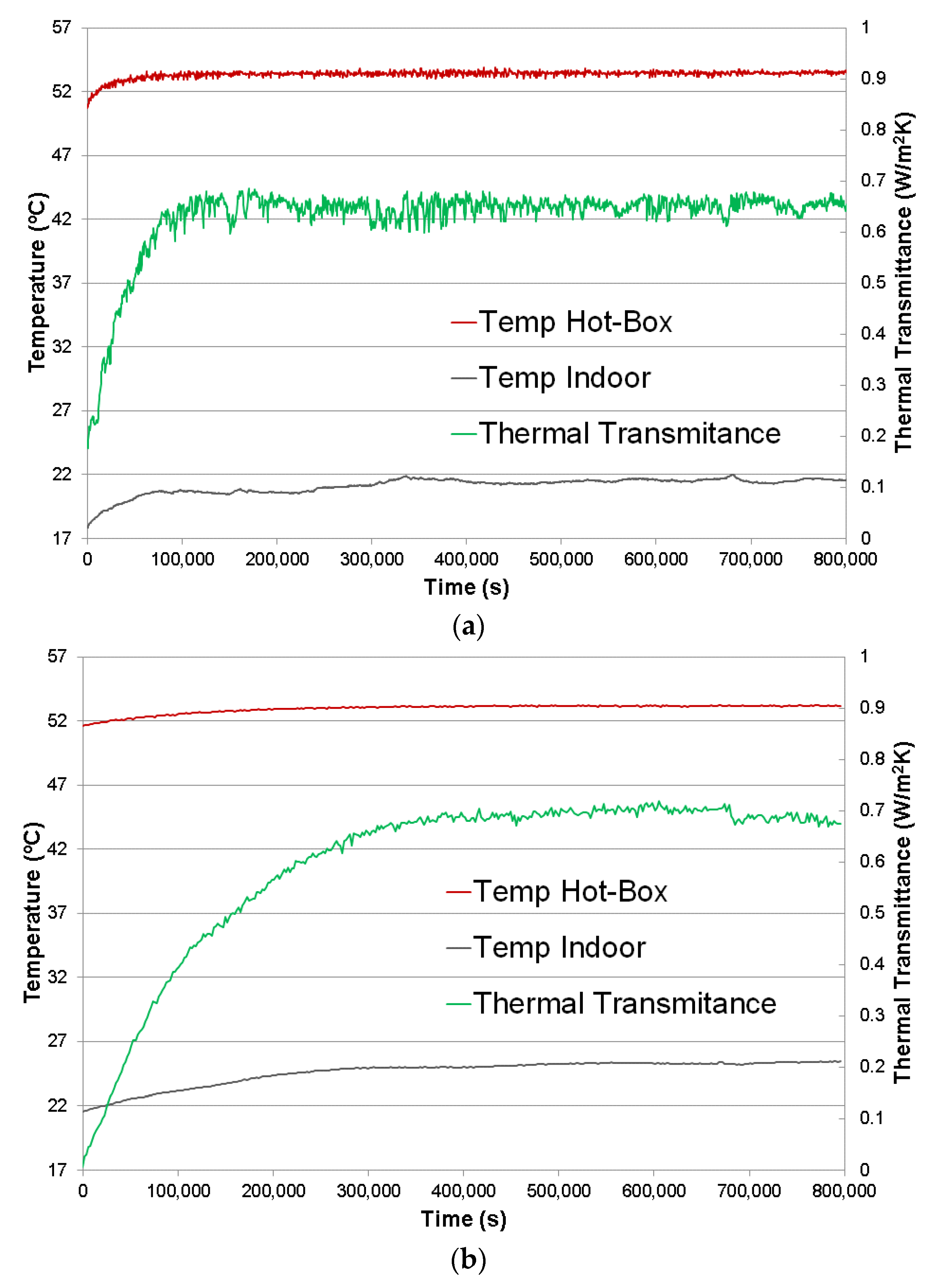
When the hot-box relative humidity is 70%, the measured thermal transmittance is 12% higher than at relative humidity of 30%. This demonstrates the importance of the moisture content in porous materials due to their hygroscopicity. In this sense, it is necessary to obtain the material thermal properties at specific humidity contents and account for the moisture transport inside multilayer walls. Moreover, the laboratory ambient conditions and the wall construction process can produce a non-uniform moisture content inside blocks and layers, affecting the thermal results.

-

Thermal transmittance in steady-state tests was higher than the empirical value calculated following the ISO 6946 standard [2], with differences ranging from 5 to 15%. Consequently, moisture content must be taken into account to obtain the thermal conductivity values of each layer of porous materials, in this case, Layer 3 (LWMA) and Layer 2 (LWBA25).

-

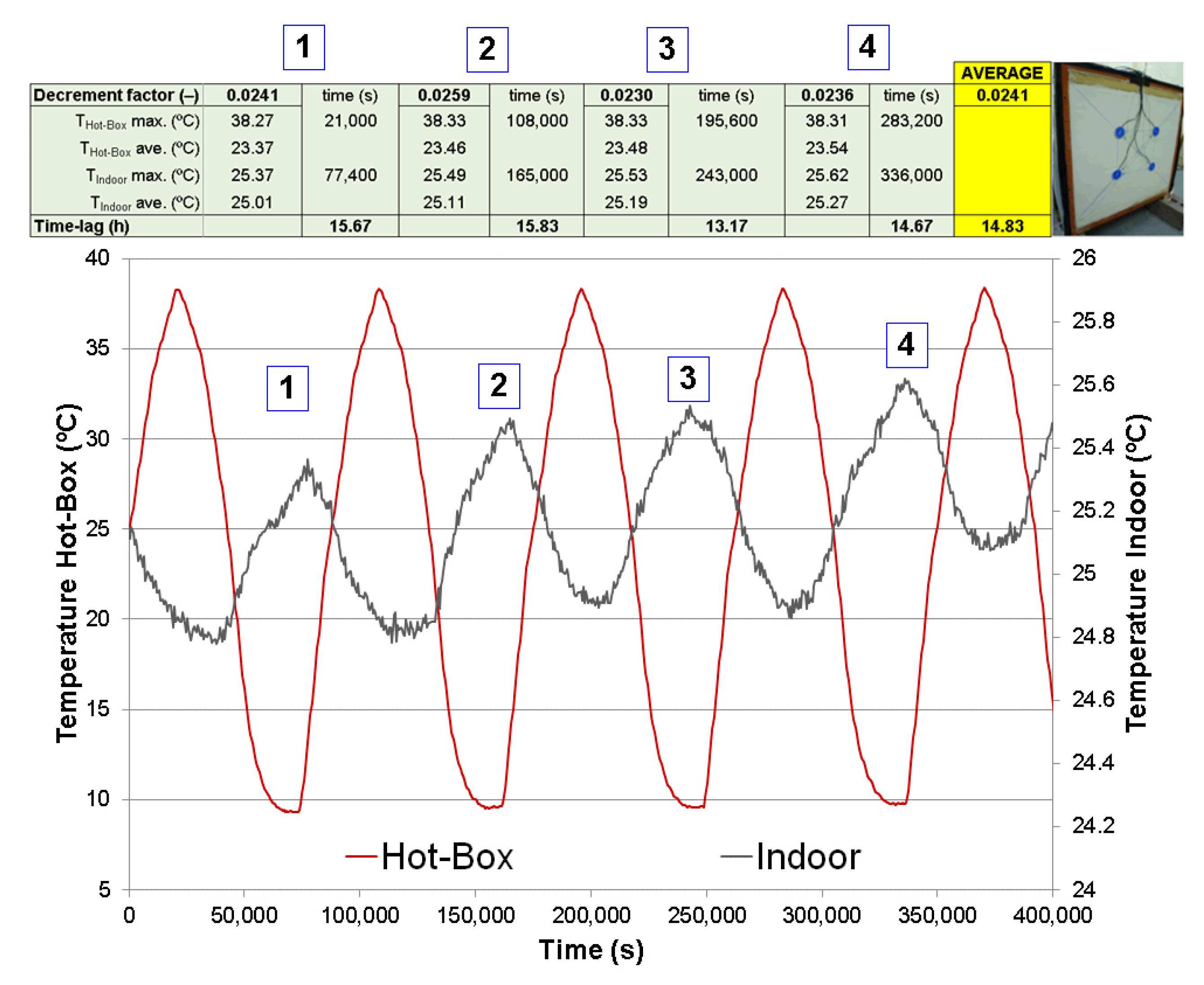
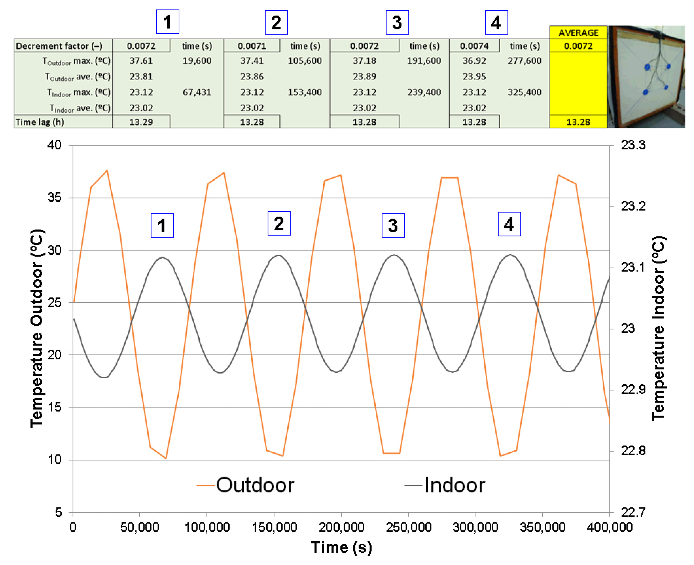
Transient thermal tests in different thermal flux directions showed significant differences in terms of time lag (1.25 h difference) and decrement factor (23% difference). Thermal inertia values were, therefore, strongly affected by the multilayer wall composition.

-

According to the thermal inertia tests, Layer 3 (LWMA) was appropriate to be exposed to the outdoor conditions. This material had the lowest density, thermal conductivity, thermal diffusivity and heat capacity in the multi-layer wall. With this configuration, a high time lag and low decrement factor were obtained, so the optimal indoor conditions were reached. Thus, materials with lower values in terms of density and thermal properties are recommended to be used at outdoor conditions.

-

Empirical dynamic thermal inertia parameters exhibited lower time lag and higher decrement factor values than the experimental results. In the empirical formulation, the decrement factor is given by the periodic thermal transmittance divided by the static thermal transmittance of layers with homogeneous materials. In this work, lightweight concrete blocks with cavities were not homogeneous. Their dynamic thermal behavior was not calculated accurately by the empirical formulation. Consequently, the ISO-13786 standard [3] provides more restrictive designs than the experimental ones, and further research is required in this field.

(2)

Numerical simulation

-

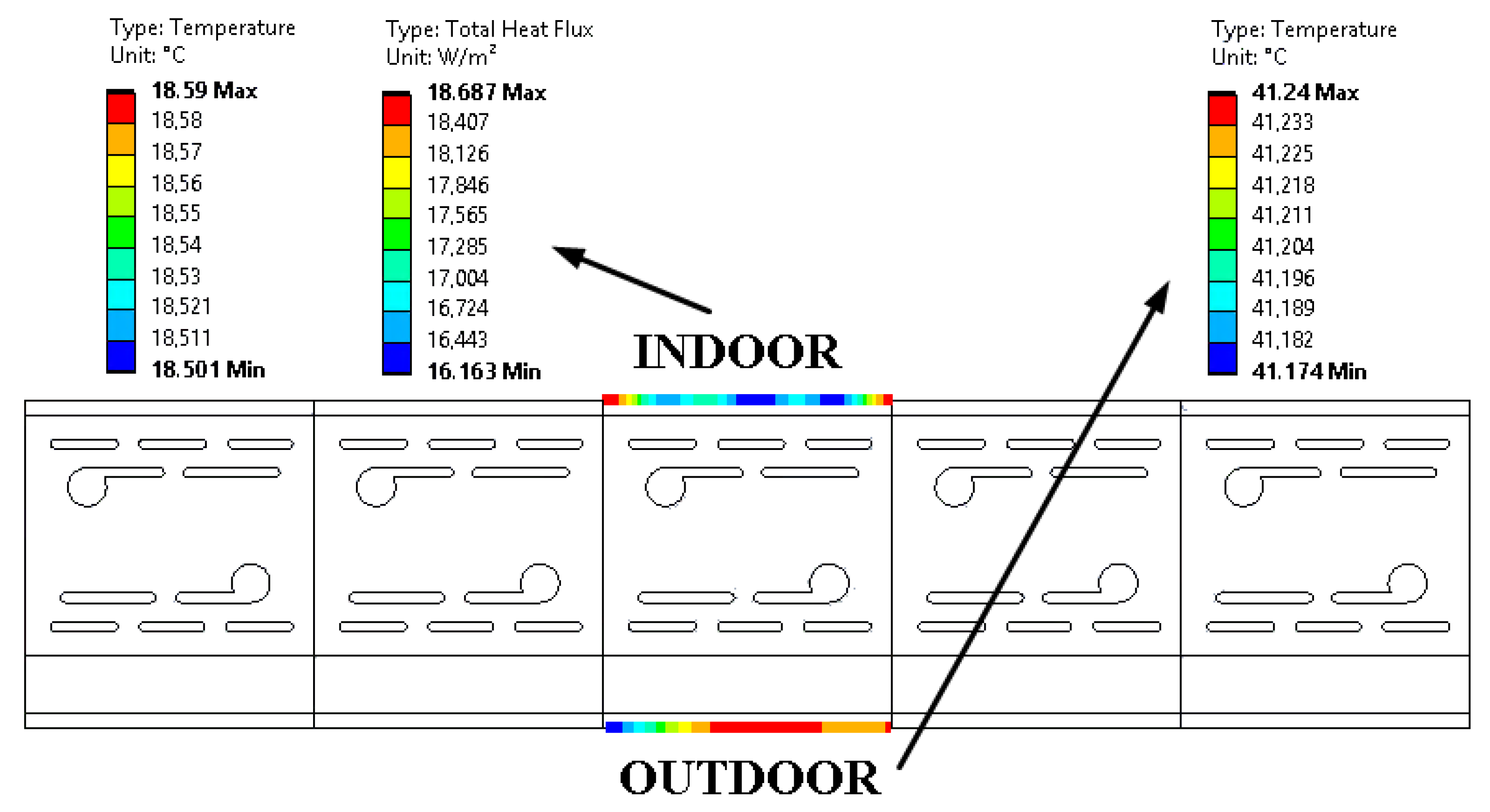
A bidimensional FEM model, including conduction, convection and radiation, was used to simulate both steady- and transient-state thermal conditions in a multi-layer wall. The average temperature and heat flux of the block in the middle of the wall was used to obtain numerical results for the thermal transmittance, time lag, and decrement factor.

-

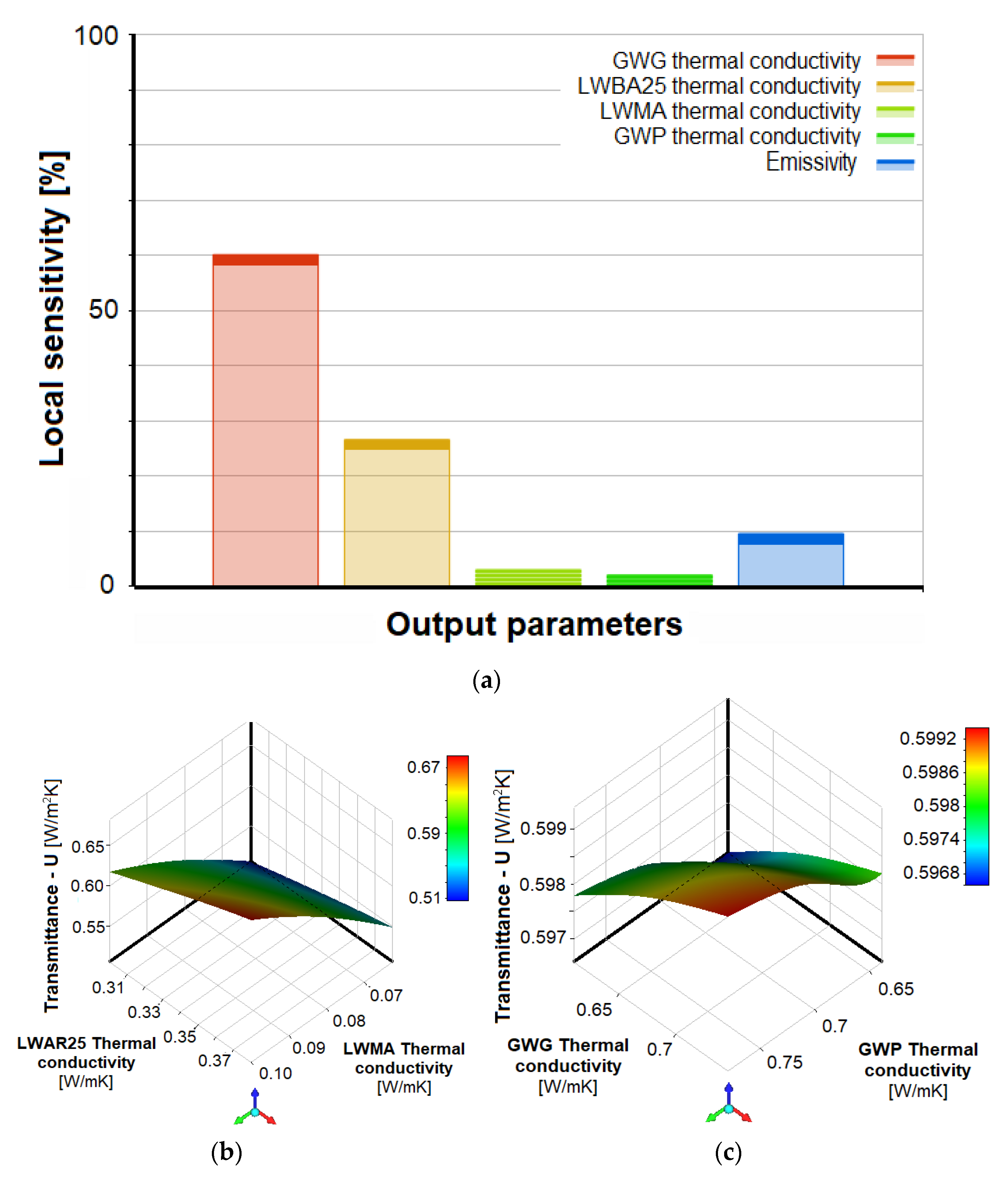
Two DOE analyses were performed to determine the most influential parameters and obtain accurate material thermal properties similar to the experimental behavior.

-

Sensitivity analysis obtained from the first DOE under steady-state conditions showed that the three most important input parameters were the thermal conductivity of Layer 3 (LWMA), the thermal conductivity of Layer 2 (LWBA25), and the emissivity of the cavities in the block.

-

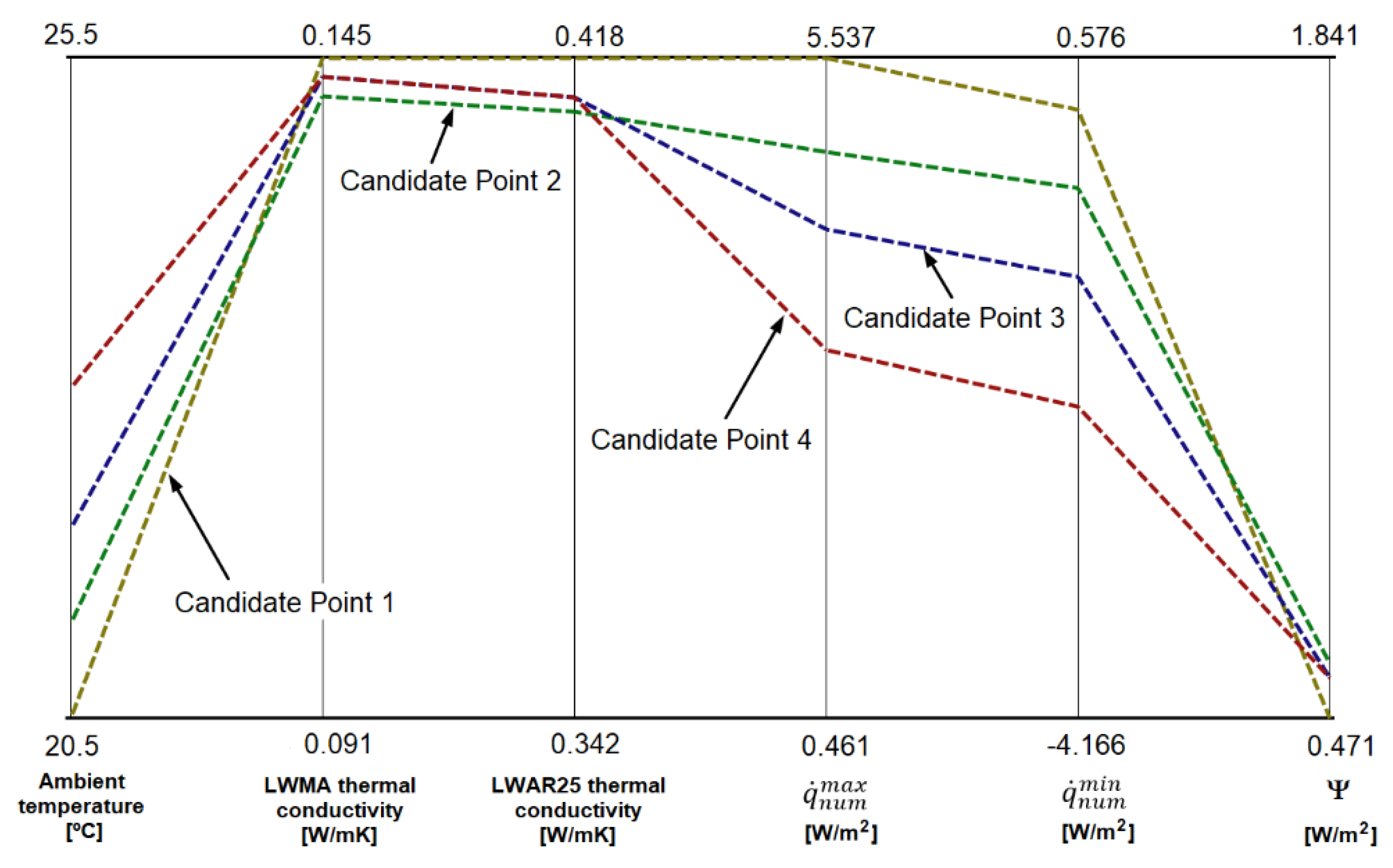
A multicriteria optimization based on second DOE analysis under transient thermal conditions was used to fit the experimental and numerical results. Thermal flux amplitude and phase Equation were used as an objective function according to Equation (11). From this optimization, the thermal conductivity of Layer 3 (LWMA) and Layer 2 (LWBA25) was obtained and used in FEM numerical models for transient- and steady-state analyses.

(3)

Numerical, empirical and experimental comparison

-

Numerical and empirical thermal transmittance results of steady-state analyses were in good agreement, showing differences of less than 6%.

-

In the transient-state numerical analysis, the temperature amplitude on the indoor face of the wall was lower than the experimental amplitude. Thus, the numerical decrement factor was lower than the value obtained experimentally or empirically. More research is necessary to better understand this effect in the transient state. In this sense, numerical FEM models could be solved with a different time discretization (smaller time steps and lower heat tolerance). In addition, dynamic heat transfer phenomena inside cavities, specifically convection and radiation, must be deeply studied.

-

Numerical and experimental time lags showed good agreement, with a difference of less than 3% between values. However, results of empirical calculations presented lower values.

This study presents a new hybrid numerical and experimental methodology based on a double DOE analyses including a multicriteria optimization over a FEM two-dimensional multi-layer wall. With the help of experimental tests, it is possible to build an accurate numerical model able to predict the steady-state and dynamic performance of walls made of porous materials, including air cavities.

Furthermore, as shown in previous works [19,20,33,34], the moisture content in porous materials has a great influence on the thermal performance of this type of lightweight concrete wall. The thermal conductivity is related to the characteristics of the pore structure and internal moisture distribution. Future studies should focus on the development of coupled numerical models, taking into account hygrothermal transport [19] and dynamic heat transfer within cavities. They could also analyze other wall compositions in order to validate the empirical formulation indicated in the Standard [3].

Finally, the numerical model developed in this work is an original contribution and a useful tool to simulate the steady-state and dynamic response of multi-layer building walls under different environmental conditions.

References

1. Li, W.; Yang, L.; Ji, Y.; Xu, P. Estimating demand response potential under coupled thermal inertia of building and air-conditioning system. Energy Build. 2019, 182, 19–29. [Google Scholar] [CrossRef]
2. ISO 6946:2017. Building Components and Building Elements—Thermal Resistance and Thermal Transmittance—Calculation Methods; ISO: Geneva, Switzerland, 2017. [Google Scholar]
3. ISO 13786:2017. Thermal Performance of Building Components—Dynamic Thermal Characteristics—Calculation Methods; ISO: Geneva, Switzerland, 2017. [Google Scholar]
4. Aste, N.; Angelotti, A.; Buzzetti, M. The influence of the external walls thermal inertia on the energy performance of well insulated buildings. Energy Build. 2009, 41, 1181–1187. [Google Scholar] [CrossRef]
5. Kossecka, E.; Kosny, J. Influence of insulation configuration on heating and cooling loads in a continuously used building. Energy Build. 2002, 34, 321–331. [Google Scholar] [CrossRef]
6. Asan, H.; Sancaktar, Y. Effects of Wall’s thermophysical properties on time lag and decrement factor. Energy Build. 1998, 28, 159–166. [Google Scholar] [CrossRef]
7. Asan, H. Effects of wall’s insulation thickness and position on time lag and decrement factor. Energy Build. 1998, 28, 299–305. [Google Scholar] [CrossRef]
8. Ozel, M.; Pihtili, K. Optimum location and distribution of insulation layers on building walls with various orientations. Build. Environ. 2007, 42, 3051–3059. [Google Scholar] [CrossRef]
9. Di Perna, C.; Stazi, F.; Casalena, A.U.; D’Orazio, M. Influence of the internal inertia of the building envelope on summertime comfort in buildings with high internal heat loads. Energy Build. 2011, 43, 200–206. [Google Scholar] [CrossRef]
10. Ng, S.-C.; Low, K.-S.; Tioh, N.-H. Thermal inertia of newspaper sandwiched aerated lightweight concrete wall panels: Experimental study. Energy Build. 2011, 43, 2956–2960. [Google Scholar] [CrossRef]
11. Jin, X.; Zhang, X.; Cao, Y.; Wang, G. Thermal performance evaluation of the wall using heat flux time lag and decrement factor. Energy Build. 2012, 47, 369–374. [Google Scholar] [CrossRef]
12. Kontoleon, K.; Theodosiou, T.; Tsikaloudaki, K. The influence of concrete density and conductivity on walls’ thermal inertia parameters under a variety of masonry and insulation placements. Appl. Energy 2013, 112, 325–337. [Google Scholar] [CrossRef]
13. Del Coz Díaz, J.; Nieto, P.G.; Biempica, C.B.; Gero, M.P. Analysis and optimization of the heat-insulating light concrete hollow brick walls design by the finite element method. Appl. Therm. Eng. 2007, 27, 1445–1456. [Google Scholar] [CrossRef]
14. Del Coz Díaz, J.; Nieto, P.G.; Rabanal, F.A.; Hernández, J.D. Non-linear thermal analysis of the efficiency of light concrete multi-holed bricks with large recesses by FEM. Appl. Math. Comput. 2012, 218, 10040–10049. [Google Scholar] [CrossRef]
15. Gencel, O.; del Coz Díaz, J.J.; Sutcu, M.; Kocyigit, F.; Rabanal, F.P.Á.; Alonso-Martínez, M.; Barrera, G.M. Thermal Performance Optimization of Lightweight Concrete/EPS Layered Composite Building Blocks. Int. J. Thermophys. 2021, 42, 1–14. [Google Scholar] [CrossRef]
16. Arendt, K.; Krzaczek, M.; Florczuk, J. Numerical analysis by FEM and analytical study of the dynamic thermal behavior of hollow bricks with different cavity concentration. Int. J. Therm. Sci. 2011, 50, 1543–1553. [Google Scholar] [CrossRef]
17. Zhang, Y.; Du, K.; He, J.; Yang, L.; Li, Y.; Li, S. Impact factors analysis on the thermal performance of hollow block wall. Energy Build. 2014, 75, 330–341. [Google Scholar] [CrossRef]
18. Soret, G.; Vacca, P.; Tignard, J.; Hidalgo, J.; Maluk, C.; Aitchison, M.; Torero, J. Thermal inertia as an integrative parameter for building performance. J. Build. Eng. 2021, 33, 101623. [Google Scholar] [CrossRef]
19. Del Coz Díaz, J.; Álvarez-Rabanal, F.; Gencel, O.; Nieto, P.G.; Alonso-Martínez, M.; Navarro-Manso, A.; Prendes-Gero, B. Hygrothermal study of lightweight concrete hollow bricks: A new proposed experimental–numerical method. Energy Build. 2014, 70, 194–206. [Google Scholar] [CrossRef]
20. Del Coz Díaz, J.J.; Rabanal, F.P.Á.; Nieto, P.J.G.; Hernández, J.D.; Soria, B.R.; Pérez-Bella, J.M. Hygrothermal properties of lightweight concrete: Experiments and numerical fitting study. Constr. Build. Mater. 2013, 40, 543–555. [Google Scholar] [CrossRef]
21. ASTM D7984—16. Standard Test Method for Measurement of Thermal Effusivity of Fabrics Using a Modified Transient Plane Source (MTPS) Instrument; ASTM: West Conshohocken, PA, USA, 2016. [Google Scholar]
22. Bull, J.W. (Ed.) Computer Analysis and Design of Masonry Structures; Saxe-Coburg Publications: Kippen, Scotland, 2016. [Google Scholar]
23. UNE-EN 1745:2020. Masonry and Masonry Products—Methods for Determining Thermal Properties; AENOR: Madrid, Spain, 2020. [Google Scholar]
24. Moaveni, S. Finite Element Analysis, Theory and Application with ANSYS; Prentice Hall: Hoboken, NJ, USA, 1999. [Google Scholar]
25. ANSYS Mechanical APDL Theory Reference. 2013. Available online: https://0-doi-org.brum.beds.ac.uk/www.ansys.com (accessed on 1 January 2020).
26. Ansys® Academic Research Mechanical, Release 19.2, Mechanical User’s Guide; ANSYS, Inc.: Canonsburg, PA, USA, 2019.
27. Madenci, E.; Guven, I. The Finite Element Method and Applications in Engineering Using Ansys®; Springer: Berlin, Germany, 2006. [Google Scholar] [CrossRef]
28. Thompson, M.; Thompson, J. ANSYS Mechanical APDL for Finite Element Analysis; Butterworth-Heinemann: New York, NY, USA, 2017. [Google Scholar]
29. Antony, J. Design of Experiments for Engineers and Scientist; Butterworth-Heinemann: New York, NY, USA, 2003. [Google Scholar]
30. Preece, D.A.; Montgomery, D.C. Design and Analysis of Experiments; John Wiley & Sons: Hoboken, NJ, USA, 1978. [Google Scholar]
31. Williams, F.A. Simplified Theory for Ignition Times of Hypergolic Gelled Propellants. J. Propuls. Power 2009, 25, 1354–1357. [Google Scholar] [CrossRef]
32. Ulgen, K. Experimental and theoretical investigation of effects of wall’s thermophysical properties on time lag and decrement factor. Energy Build. 2002, 34, 273–278. [Google Scholar] [CrossRef]
33. Ökten, K.; Özdemir, M. Experimental Investigation of the Performance of Porous Insulation Materials Under Temporary Humidity. J. Thermophys. Heat Transf. 2021, 35, 179–186. [Google Scholar] [CrossRef]
34. Wang, Y.; Zhao, Z.; Liu, Y.; Wang, D.; Ma, C.; Liu, J. Comprehensive correction of thermal conductivity of moist porous building materials with static moisture distribution and moisture transfer. Energy 2019, 176, 103–118. [Google Scholar] [CrossRef]
Figure 1. Thermal conductivity tests: (a) GWG; (b) LWMA; (c) GWP; and (d) experimental set-up.
Applsci 11 05008 g001
Figure 2. Transient thermal inertia set-up: (a) Direction 1 and (b) Direction 2.
Applsci 11 05008 g002
Figure 3. Geometrical model and material layer identification: (1) GWG, (2) LWBA25, (3) LWMA and (4) GWP.
Applsci 11 05008 g003
Figure 4. Steady-state test results at (a) 30% and (b) 70% relative humidity.
Applsci 11 05008 g004
Figure 5. Transient-state test results showing the decrement factor and time lag in thermal flux Direction 1.
Applsci 11 05008 g005
Figure 6. Transient-state test results showing the decrement factor and time lag in thermal flux Direction 2.
Applsci 11 05008 g006
Figure 7. Transient experimental results showing temperature and heat fluxes in thermal flux Direction 2.
Applsci 11 05008 g007
Figure 8. DOE results: (a) Sensitivity analysis of parameters and response surfaces of (b) LWAR25 and LWMA thermal conductivities vs. thermal transmittance and (c) GWG and GWP thermal conductivities vs. thermal transmittance.
Applsci 11 05008 g008
Figure 9. Candidate point results from the optimization based on DOE.
Applsci 11 05008 g009
Figure 10. Indoor and outdoor heat flux and temperature distribution at the center of the wall.
Applsci 11 05008 g010
Figure 11. Numerical analysis in thermal flux Direction 2, showing the transient results of the decrement factor and time lag at the central location of the wall.
Applsci 11 05008 g011
Figure 12. Comparison of thermal flux results obtained using experimental and numerical methods.
Applsci 11 05008 g012
Figure 13. Comparison of indoor wall face temperature experimental and numerical results.
Applsci 11 05008 g013