3D In Situ Stress Estimation by Inverse Analysis of Tectonic Strains

Abstract

The determination of a 3D engineering-scale in situ stress field is essential in underground rock mechanics and engineering. The inverse analysis method is a useful technique to determine the in situ stress around the zone of interest. This paper presents a new approach with tectonic strains based on traditional stress-based or displacement-based inverse analysis. In this approach, there are only six tectonic strain variables at the boundary to be optimized, which does not need to select the stress or displacement boundary conditions as the traditional inverse analysis. Therefore, the proposed approach has a better clarity. The proposed approach is applied to the determination of the engineering-scale in situ stress of the underground powerhouses of the Three Gorges Project, and the results are compared with those obtained by traditional approaches. The comparison further shows that the proposed method has better accuracy than traditional methods.

1. Introduction

The magnitude, orientation and distribution of in situ stress are of fundamental importance for not only design and stability assessment in underground rock engineering [1,2] but also the assessment of the excavation-induced rock behaviors, such as the deformation, disturbed zone, damage, permeability variation, etc. [3,4,5]. Field measurement to obtain in situ stress directly is costly and time-consuming. In engineering practice, only a limited number of points in a region are chosen to perform in situ stress measurement [6,7]. Theoretically, the in situ stress determined at the limited number of points only reflects local stress states near the testing points, and practically, the in situ stress in the region that includes the testing points are estimated by forward geomechanical modeling and inverse analysis [8,9,10,11,12].

The traditional stress-based and displacement-based approaches are always used in simulating an in situ stress field, however, the selection of the boundary mode is still the key problem for both approaches. In the stress- or displacement-based approach, there are about 14 variables for only the linear boundary mode, and there will be more variables in quadric or other complicated boundary conditions. Nevertheless, the resulting high dimensionality of the optimization process will make it extremely difficult to solve the problem in an efficient way. Furthermore, more complicated expression for stress or displacement boundary mode does not necessarily lead to a better assessment for in situ stress field and it is not taken into account for the connection between the normal and shear stress or displacement on boundaries.

To date, there are at least two challenges in determining in situ stress by forward modeling and inverse analysis. The first challenge is the ambiguity and uncertainty of assumptions in the distribution of either tectonic stress or tectonic displacement at the boundary in forward modeling [13,14,15,16]. In forward modeling, either a stress or displacement boundary condition needs to be assumed to obtain the in situ stress. However, for either of the boundary conditions, an assumption of linear distribution or quadratic distribution leads to the different final results of the engineering-scale in situ stress estimation. It is unclear which assumption leads to a more accurate estimation of the engineering-scale in situ stress.

The second challenge is the high dimensionality of input and output variables involved in the inverse analysis [17]. Here, inverse analysis is mainly an optimization process with computational efforts growing exponentially with dimensions [18]. In the aforementioned stress- or displacement-based approach, there are about 10 variables for only linear boundary mode, and there will be more variables in quadric or other complicated boundary conditions, whereas there are usually multiple local in situ stress states as multi-objectives, and the resulting high dimensionality of the optimization process will make it extremely difficult to solve the problem in an efficient and accurate way.

It is well known that, from a geological point of view, the in situ stress field should be an unsteady stress field and changes with time, however, from the point view of engineering construction, the in situ stress field can be considered as a relatively steady stress field. A large number of practical projects indicate that the region of interest in the project is mostly controlled by a big tectonic stress field caused by modern crustal movement and all kinds of tectonic activities [19,20], and except for the individual place largely influenced by local stress, the directions of principal stresses in most regions are roughly consistent. Therefore, it can be considered that tectonic movement is relatively uniform on the boundaries of the region of interest and the tectonic stress field can be simulated by optimizing the regional tectonic strain of the boundary.

To address these challenges, this paper presents a new approach considering the regional tectonic strain as an optimized variable in order to effectively reduce the high dimensionality of the problem. According to geological conditions of the Three Gorges Project, the main faults and joints were taken into account and the 3-D finite element model was established. Compared with the traditional inverse analysis method, the boundary conditions containing tectonic strain are applied in the 3-D calculating model during back analysis, and only six strain variables need to be optimized in the proposed method. The computing results demonstrate that this approach is of efficiency in simulating the in situ stress of the Three Gorges Project.

2. Inverse Analysis for In Situ Stress Determination

Boundary conditions are crucial for a definite solution of the governing equation. For any problem, boundary conditions are required. The processing of boundary conditions directly affects the accuracy of calculation results.

Stress or displacement boundary conditions around the region of interest can determine the engineering-scale in situ stress field. For traditional inverse analysis about an in situ stress field, the purpose is to find the best-fit boundary stress or displacement distribution of the zone of interest. Optimization algorithms are usually used to determine the best-fit boundary conditions. With respect to the objective function for an optimization algorithm, it can be established by the errors between the field test values and the calculated values in the limited testing points of the zone of interest. The calculated values can be obtained by given boundary conditions during the optimizing process. Therefore, the in situ stress field can be inversely analyzed by optimizing engineering-scale boundary conditions and determined through best-fit boundary conditions. In this section, two traditional inverse analysis approaches are introduced [11,16,21], and furthermore, in order to overcome the drawbacks of traditional approaches, a new approach is proposed and explained.

2.1. Tectonic Stress-Based Approach

The in situ stress field has been considered as the superposition of gravity and tectonic stress field. Therefore, it can be expressed as Equation (1):

$$\sigma ={\sigma }^0+{\sigma }^t$$

(1)

where $\sigma$ is the in situ stress at any point, ${\sigma }^0$ is the gravity stress, which can be easily calculated by numerical analysis, and it can be recognized as a known quantity, and ${\sigma }^t$ is the tectonic stress.

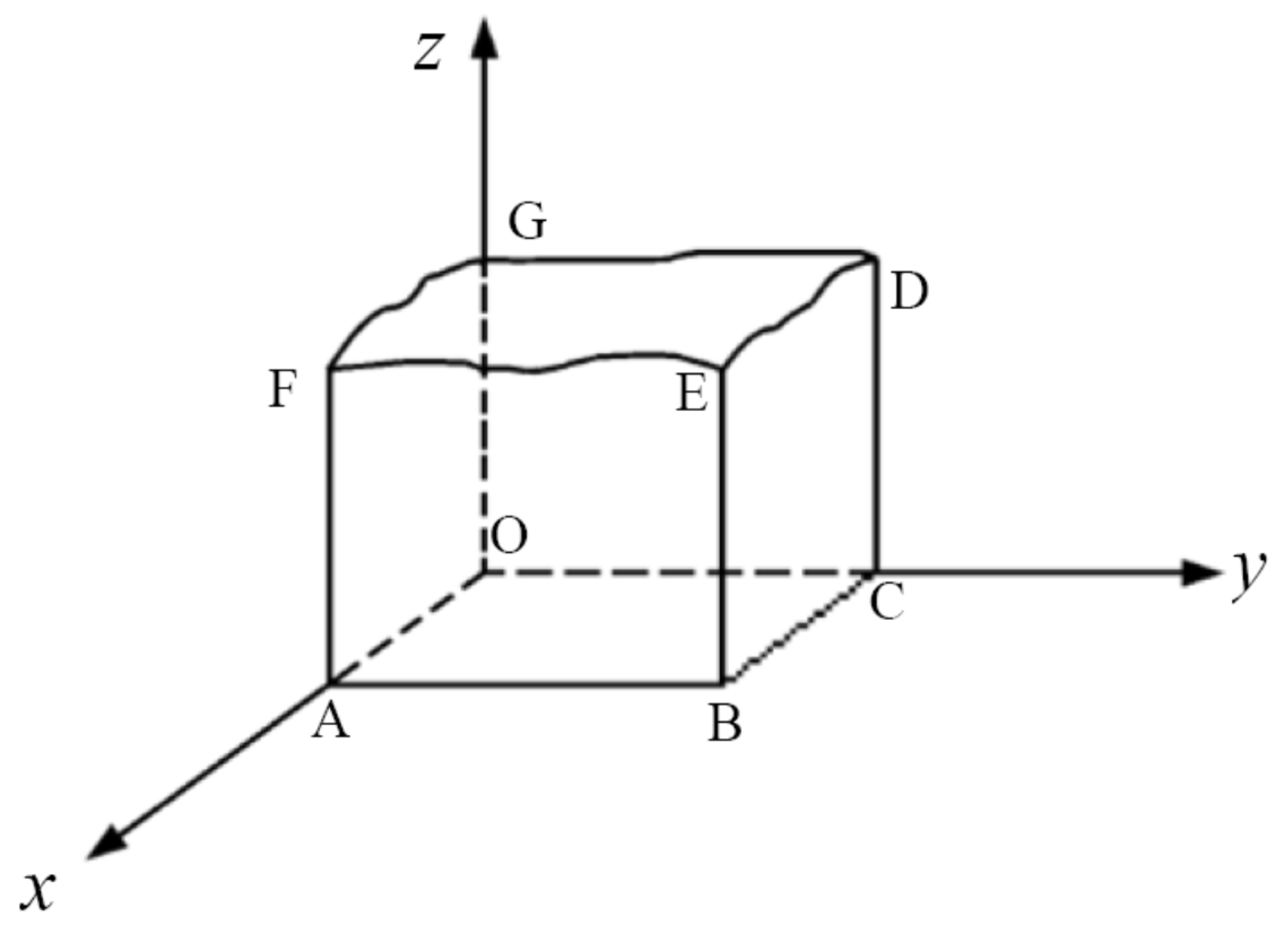
Figure 1 demonstrates a simple calculating model, where the bottom is fixed and all lateral boundary conditions are normally restrained, and only the gravity load is applied. With this model, the gravity stress field can be calculated based on the theory of elasticity.

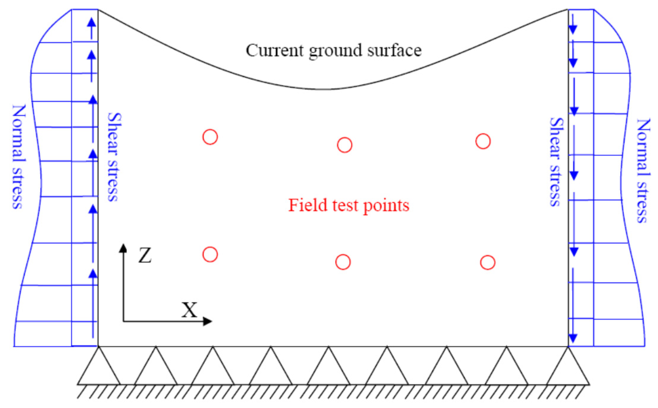
Figure 2 shows a 2-D calculating model to calculate normal tectonic stress ${\sigma }^t$, where in X–Z section, the normal tectonic stress on the boundary can be considered as a linear expression (Equation (2)), or quadratic expression (Equation (3)) of the coordinates on the boundaries. As the coordinate X is the constant, the coordinate Z changes with the location on the boundaries. Therefore, the normal tectonic stress can be expressed as the function of the coordinate Z (Equation (4)):

$${\sigma }_{\mathit{n}}={\mathit{a}}_0+{\mathit{a}}_1\times \mathit{z}$$

(2)

$${\sigma }_{\mathit{n}}={\mathit{a}}_0+{\mathit{a}}_1\times \mathit{z}+{\mathit{a}}_2\times {\mathit{z}}^2$$

(3)

$${\sigma }_{\mathit{n}}=\mathit{f}({\mathit{a}}_0,{\mathit{a}}_1,{\mathit{a}}_2)$$

(4)

where ${\mathit{a}}_0,{\mathit{a}}_1,{\mathit{a}}_2$ are just unknown coefficients which need to be solved by inverse analysis and have no physical meaning. Similarly, for the shear stress on boundaries (Figure 2), Equation (5) is the quadratic expression, in which the coordinate X is constant and the coordinate Z can be obtained on the basis of the location on the boundaries. Additionally, the shear stress should be zero at the intersection point between the ground surface and the boundary because of the equivalent theorem of shearing stress. For the direction of the shear stress on both sides in Figure 2, it needs to be clarified that it is just one possibility of tectonic stress in practical engineering, which is possible since they have the same direction on both sides of the model and the direction of the shear stress can be determined by optimizing the stress-based boundary conditions. During the optimization process, the direction of the shear stress is considered by the positive or negative value of the shear stress. Therefore, the shear stress can still be considered as the function of the coordinate Z (Equation (6)):

$${\sigma }_{\tau }={\mathit{b}}_1\times \mathit{z}+{\mathit{b}}_2\times {\mathit{z}}^2$$

(5)

$${\sigma }_{\tau }=\mathit{f}({\mathit{b}}_1,{\mathit{b}}_2)$$

(6)

Here, just like in Equation (4), ${\mathit{b}}_1$ and ${\mathit{b}}_2$ are also just coefficients and need to be solved by inverse analysis.

Therefore, combining the normal and shear stress boundary conditions, the boundary mode for this method can be summarized as Equation (7):

$$\mathit{f}=\mathit{f}({\mathit{a}}_0,{\mathit{a}}_1,{\mathit{a}}_2,{\mathit{b}}_1,{\mathit{b}}_2)$$

(7)

For the 2-D calculating model, it can be seen that there are three variables in linear boundary mode and five variables in quadratic boundary mode. However, there will be more variables in the 3-D calculating model.

For the 3-D calculating model in Figure 1, on the boundary ABEF or OCDG, the normal stress can be linearly expressed as Equation (8). Nevertheless, the shear stress on boundary ABEF or OCDG, can be divided into two types, one direction is along axis Y, and the other is along axis Z. The shear stress along axes Yand Z can be, respectively, considered as Equations (9) and (10):

$${\sigma }_{\mathit{n}}={\mathit{a}}_0+{\mathit{a}}_1\times \mathit{y}+{\mathit{a}}_2\times \mathit{z}$$

(8)

$${\sigma }_{\tau \mathrm{y}}={\mathit{b}}_1\times \mathit{y}+{\mathit{b}}_2\times \mathit{z}$$

(9)

$${\sigma }_{\tau \mathrm{z}}={\mathit{c}}_1\times \mathit{y}+{\mathit{c}}_2\times \mathit{z}$$

(10)

Similarly, for boundary BCDE or AOGF, the normal stress can still be expressed as Equation (8) with different coefficients ${\mathit{d}}_0,{\mathit{d}}_1,{\mathit{d}}_2$, and the shear stress along axis X and axis Z can also be considered as Equations (9) and (10) with different coefficients ${\mathit{e}}_1,{\mathit{e}}_2,{\mathit{e}}_3,{\mathit{e}}_4.$ Therefore, the boundary mode for the 3-D calculating model can be summarized as Equation (11):

$$\mathit{f}=\mathit{f}({\mathit{a}}_0,{\mathit{a}}_1,{\mathit{a}}_2,{\mathit{b}}_1,{\mathit{b}}_2,{\mathit{c}}_1,{\mathit{c}}_2,{\mathit{d}}_0,{\mathit{d}}_1,{\mathit{d}}_2,{\mathit{e}}_1,{\mathit{e}}_2,{\mathit{e}}_3,{\mathit{e}}_4)$$

(11)

where, just like the coefficients ${\mathit{a}}_0$, ${\mathit{a}}_1$, ${\mathit{a}}_2$ in Equation (4) and the coefficients ${\mathit{b}}_1$, ${\mathit{b}}_2$ in Equation (6), ${\mathit{c}}_1$, ${\mathit{c}}_2$, ${\mathit{d}}_0$, ${\mathit{d}}_1$, ${\mathit{e}}_1$, ${\mathit{e}}_2$, ${\mathit{e}}_3$ and ${\mathit{e}}_4$ are also unknown coefficients and need to be solved by inverse analysis using optimization algorithm.

Based on the above analysis, for the strictly linear expression of stress boundary condition in the 3-D calculating model in Figure 1, there are seven variables on each boundary, and apart from the bottom boundary, there are about 28 variables for linear stress expression on the boundaries BCDE, ABEF, AOGF and OCDG. In order to strictly meet the force equilibrium applied on boundaries for whole model, in inverse analysis, the stress boundary is usually simply dealt with as the follows: the normal and shear stress conditions are applied to the boundaries BCDE and ABEF, the boundaries AOGF and OCDG are normally constrained, and the bottom ones are fixed. Mostly, multiple regression approach is utilized to solve the best-fit boundary, especially the linear regression approach [17].

It can be seen that for linear expressions of stress boundary mode in 3-D calculating model, there are seven variables on each boundary BCDE and ABEF, and in total, 14 variables need to be solved by linear regression approach, however, more variables will appear in complex expressions for stress boundary mode.

In order to obtain a reasonable in situ stress field, the best-fit stress boundary condition must be determined by using the optimization algorithm, such as the simplex method, neural network, genetic algorithm [22], and surrogate model accelerated random search [17]. Generally, the objective function needs to be established based on the measured values and calculated values, as Equation (12). For the optimization algorithm, if the variables are less than 10, the simplex algorithm can be available to obtain the rational results, or else the global optimization algorithm should be more effective than the simplex algorithm:

$$F=\min {\displaystyle \sum _{j=1}^m{\displaystyle \sum _{k=1}^6}{\Vert {\sigma }_{jk}-{\hat{\sigma }}_{jk}\Vert }_2}$$

(12)

where m is the number of measured points in the field test, for Figure 2, m = 6. ${\Vert \Vert }_2$ is the 2-norm of stress tensor, ${\hat{\sigma }}_{j\mathrm{k}}$ stands for the k component of the measured stress tensor at point j, and ${\sigma }_{jk}$ is the corresponding calculated value at point j.

For a stress-based approach, the key problem is to select the stress boundary mode, and different boundary modes determine different in situ stress fields. It needs to be noted that a more complicated expression of stress boundary mode does not necessarily lead to a better estimation of an in situ stress field. However, in an optimization algorithm, more variables require exponentially increased computational effort.

2.2. Tectonic Displacement-Based Approach

Similarly to the concept that the in situ stress field is composed of the gravity and tectonic stress field, the displacement field on the boundary of a region can also be assumed as the combination of the displacements induced by both gravity and tectonic stress fields. The displacement $\left(u,v,w\right)$ on the boundary of 3-D calculating model can be expressed as Equation (13):

$$\left(\begin{array}{c}u\\ v\\ w\end{array}\right)=\left(\begin{array}{c}{u}^0\\ v^0\\ w^0\end{array}\right)+\left(\begin{array}{c}{u}^t\\ v^t\\ w^t\end{array}\right)$$

(13)

where $\left(u^0,v^0,w^0\right)$ is the displacement of corresponding X, Y and Z axes at any point on the lateral boundary induced by the gravity stress field in the 3-D calculating model and $\left(u^t, v^t,w^t\right)$ is the displacement induced by tectonic stress field.

For the displacement $\left(u^0, v^0,w^0\right)$ at boundary, it is easy to obtain the gravity stress field based on the theory of elasticity.

For the tectonic displacement $\left(u^t, v^t,w^t\right)$ at the boundary, it can be explained by a 3-D calculating model (Figure 3). For boundaries ABEF and OCDG, the normal displacement $u_n$ can be assumed to be Equation (14). For the shear displacement, there are also two types of displacement $u_{\tau y}$ and $u_{\tau z}$ in red color, and they can be expressed as Equations (15) and (16):

$${\mathit{u}}_{\mathit{n}x}={\mathit{a}}_0+{\mathit{a}}_1\times \mathit{y}+{\mathit{a}}_2\times \mathit{z}$$

(14)

$${\mathit{u}}_{\tau \mathit{y}}={\mathit{b}}_1\times \mathit{y}+{\mathit{b}}_2\times \mathit{z}$$

(15)

$${\mathit{u}}_{\tau \mathit{z}}={\mathit{c}}_1\times \mathit{y}+{\mathit{c}}_2\times \mathit{z}$$

(16)

For boundaries BCDE and AOGF, similarly to Equations (14)–(16), Equation (17) can account for the normal displacement $u_{ny}$, and the Equations (18) and (19) are for shear displacements $u_{\tau \mathrm{x}}$ and $u_{\tau \mathrm{z}}$, as shown in Figure 3:

$${\mathit{u}}_{\mathit{n}x}={\mathit{d}}_0+{\mathit{d}}_1\times \mathit{y}+{\mathit{d}}_2\times \mathit{z}$$

(17)

$${\mathit{u}}_{\tau \mathit{y}}={\mathit{e}}_1\times \mathit{y}+{\mathit{e}}_2\times \mathit{z}$$

(18)

$${\mathit{u}}_{\tau \mathit{z}}={\mathit{e}}_3\times \mathit{y}+{\mathit{e}}_4\times \mathit{z}$$

(19)

Once the displacement boundary conditions are set, the rest of the forward modeling process is the same as the stress boundary-based approach. It should be noted that this approach is still more extensively applied than stress-based approach, because the stress is not usually consistent on the boundary when there is different rock mass or fault on the boundary.

2.3. Proposed Tectonic-Strain-Based Approach

Based on the knowledge of practical engineering, a new approach is proposed in this paper for the inverse analysis of the in situ stress field, and only the tectonic strain on boundaries can be assumed to be uniform. Then, the tectonic displacement on the boundary can be expressed in the form of engineering-scale tectonic strain as in Equation (20):

$$\left(\begin{array}{c}{u}^t\\ v^t\\ w^t\end{array}\right)=\left[\begin{array}{ccc}{\epsilon }_x^t& {\epsilon }_{xy}^t& {\epsilon }_{xz}^t\\ {\epsilon }_{yx}^t& {\epsilon }_y^t& {\epsilon }_{yz}^t\\ {\epsilon }_{zx}^t& {\epsilon }_{zy}& {\epsilon }_z^t\end{array}\right]\left(\begin{array}{c}x\\ y\\ z\end{array}\right)$$

(20)

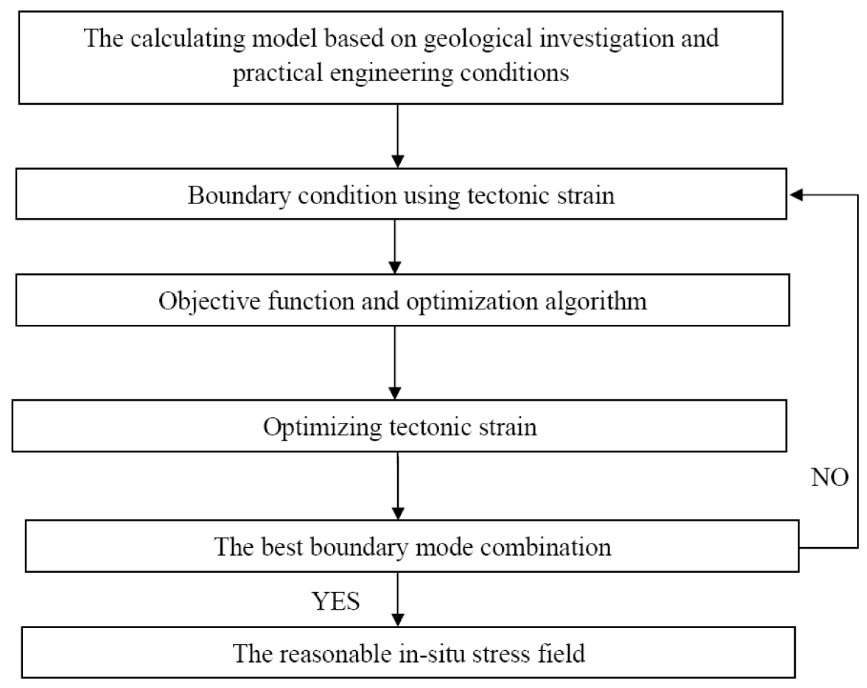
where $\left[\begin{array}{ccc}{\epsilon }_x^t& {\epsilon }_{xy}^t& {\epsilon }_{xz}^t\\ {\epsilon }_{yx}^t& {\epsilon }_y^t& {\epsilon }_{yz}^t\\ {\epsilon }_{zx}^t& {\epsilon }_{zy}& {\epsilon }_z^t\end{array}\right]$ is the regional tectonic strain tensor. As it cannot be directly applied on boundaries for strain condition, it has to be transformed to other conditions, such as stress boundary condition and displacement boundary condition. Due to the easiness of applying displacement boundary, here the engineering-scale tectonic strain can be transformed into displacement condition. Then, if the engineering-scale strain on the boundary is known, the total displacement on boundaries can be determined in Equation (21). Therefore, the calculating process of this approach can be demonstrated as in Figure 4:

$$\left(\begin{array}{c}\mathit{u}\\ \mathit{v}\\ \mathit{w}\end{array}\right)=\left(\begin{array}{c}{\mathit{u}}^0\\ {\mathit{v}}^0\\ {\mathit{w}}^0\end{array}\right)+\left(\begin{array}{c}{\mathit{u}}^{\mathit{t}}\\ {\mathit{v}}^{\mathit{t}}\\ {\mathit{w}}^{\mathit{t}}\end{array}\right)=\left(\begin{array}{c}{\mathit{u}}^0\\ {\mathit{v}}^0\\ {\mathit{w}}^0\end{array}\right)+\left[\begin{array}{ccc}{\mathit{\epsilon }}_{\mathit{x}}^{\mathit{t}}& {\mathit{\epsilon }}_{\mathit{x}\mathit{y}}^{\mathit{t}}& {\mathit{\epsilon }}_{\mathit{x}\mathit{z}}^{\mathit{t}}\\ {\mathit{\epsilon }}_{\mathit{y}\mathit{x}}^{\mathit{t}}& {\mathit{\epsilon }}_{\mathit{y}}^{\mathit{t}}& {\mathit{\epsilon }}_{\mathit{y}\mathit{z}}^{\mathit{t}}\\ {\mathit{\epsilon }}_{\mathit{z}\mathit{x}}^{\mathit{t}}& {\mathit{\epsilon }}_{\mathit{z}\mathit{y}}& {\mathit{\epsilon }}_{\mathit{z}}^{\mathit{t}}\end{array}\right]\left(\begin{array}{c}\mathit{x}\\ \mathit{y}\\ \mathit{z}\end{array}\right)$$

(21)

where $\left(u^0,v^0,w^0\right)$ and $\left(u^t,v^t,w^t\right)$ are defined in Equation (20), $\left(u^0,v^0,w^0\right)$ is the displacement at any point on the lateral boundary induced by gravity stress field in the 3-D calculating model, and $\left(u^t,v^t,w^t\right)$ is the displacement induced by the tectonic stress field. Taking the 3-D model in Figure 3 as an example, on the lateral boundaries, the tectonic displacements along the axis X, Y and Z, were, respectively, applied as the Equations (22)–(24) based on the proposed approach:

$${\mathit{u}}^{\mathit{t}}={\mathit{\epsilon }}_{\mathit{x}}^{\mathit{t}}\mathit{x}+{\mathit{\epsilon }}_{\mathit{x}\mathit{y}}^{\mathit{t}}\mathit{y}+{\mathit{\epsilon }}_{\mathit{x}\mathit{z}}^{\mathit{t}}\mathit{z}$$

(22)

$${\mathit{v}}^{\mathit{t}}={\mathit{\epsilon }}_{\mathit{y}\mathit{x}}^{\mathit{t}}\mathit{x}+{\mathit{\epsilon }}_{\mathit{y}}^{\mathit{t}}\mathit{y}+{\mathit{\epsilon }}_{\mathit{y}\mathit{z}}^{\mathit{t}}\mathit{z}$$

(23)

$${\mathit{w}}^{\mathit{t}}={\mathit{\epsilon }}_{\mathit{z}\mathit{x}}^{\mathit{t}}\mathit{x}+{\mathit{\epsilon }}_{\mathit{z}\mathit{y}}^{\mathit{t}}\mathit{y}+{\mathit{\epsilon }}_{\mathit{z}}^{\mathit{t}}\mathit{z}$$

(24)

From Equations (21)–(24), it was demonstrated that the coordinates X, Y, and Z are known based on the location of the boundaries and only the tectonic strain tensor was unknown in Equations (21)–(24), and based on the symmetry characteristic of the tectonic strain tensor, the strain ${\mathit{\epsilon }}_{\mathit{z}\mathit{x}}^{\mathit{t}}$ = ${\mathit{\epsilon }}_{\mathit{x}\mathit{z}}^{\mathit{t}}$, ${\mathit{\epsilon }}_{\mathit{z}\mathit{y}}^{\mathit{t}}$ = ${\mathit{\epsilon }}_{\mathit{y}\mathit{z}}^{\mathit{t}}$ and ${\mathit{\epsilon }}_{\mathit{y}\mathit{x}}^{\mathit{t}}$ = ${\mathit{\epsilon }}_{\mathit{x}\mathit{y}}^{\mathit{t}}$, therefore, there are only six unknown variables in Equations (21)–(24), and they need to be solved by inverse analysis.

Based on aforementioned analysis, the tectonic strain tensor containing six unknown variables can be expressed as Equation (25). Therefore, for the proposed approach, the displacement boundary conditions can be applied on each lateral boundary as Equations (26)–(28), Equation (26) is for the displacement along the axis X, Equation (27) is along the axis Y, and the Equation (28) is along the axis Z on each lateral boundary ABEF, BCDE, CODG and AOGF in Figure 3. Therefore, in this approach the displacement boundary mode for the 3-D calculating model can be summarized as Equation (29):

$$\left[\begin{array}{ccc}{\mathit{\epsilon }}_{\mathit{x}}^{\mathit{t}}& {\mathit{\epsilon }}_{\mathit{x}\mathit{y}}^{\mathit{t}}& {\mathit{\epsilon }}_{\mathit{x}\mathit{z}}^{\mathit{t}}\\ {\mathit{\epsilon }}_{\mathit{y}\mathit{x}}^{\mathit{t}}& {\mathit{\epsilon }}_{\mathit{y}}^{\mathit{t}}& {\mathit{\epsilon }}_{\mathit{y}\mathit{z}}^{\mathit{t}}\\ {\mathit{\epsilon }}_{\mathit{z}\mathit{x}}^{\mathit{t}}& {\mathit{\epsilon }}_{\mathit{z}\mathit{y}}& {\mathit{\epsilon }}_{\mathit{z}}^{\mathit{t}}\end{array}\right]=\left[\begin{array}{ccc}{\mathit{a}}_0& {\mathit{a}}_1& {\mathit{a}}_2\\ {\mathit{a}}_1& {\mathit{b}}_0& {\mathit{b}}_1\\ {\mathit{a}}_2& {\mathit{b}}_1& {\mathit{c}}_0\end{array}\right]$$

(25)

$$\mathit{u}={\mathit{u}}_0+{\mathit{a}}_{0}x+{\mathit{a}}_1\mathit{y}+{\mathit{a}}_2\mathit{z}$$

(26)

$$\mathit{v}={\mathit{v}}_0+{\mathit{a}}_{1}x+{\mathit{b}}_0\mathit{y}+{\mathit{b}}_1\mathit{z}$$

(27)

$$\mathit{w}={\mathit{w}}_0+{\mathit{a}}_{2}x+{\mathit{b}}_1\mathit{y}+{\mathit{c}}_0\mathit{z}$$

(28)

$$\mathit{f}=\mathit{f}({\mathit{a}}_0,{\mathit{a}}_1,{\mathit{a}}_2,{\mathit{b}}_0,{\mathit{b}}_1,{\mathit{c}}_0)$$

(29)

where ${\mathit{a}}_0$, ${\mathit{a}}_1$, ${\mathit{a}}_2$, ${\mathit{b}}_0$, ${\mathit{b}}_1$, ${\mathit{c}}_0$ are just unknown coefficients, i.e., tectonic strains, and need to be solved by inverse analysis using the optimization algorithm.

In this approach, the engineering-scale strain on lateral boundaries is assumed as the variables, and Equations (26)–(28) are considered as the displacement boundary conditions applied in the 3-D simulating model. In order to find the reasonable tectonic strain on boundaries, the objective function needs to be established. In practical engineering, the objective function is generally based on the measured values at limited test points and calculated values at the corresponding points, and the minimum of the 2-norm of a stress tensor composed of the difference values between the measured values and calculated values can be made the objective function. Additionally, using the optimization algorithm, the tectonic strain would be automatically optimized until the objective function is converged as the best-fit function. For the optimization algorithm, the mathematic software MATLAB has a global optimization toolbox including a simplex algorithm, global search algorithm, pattern search method, genetic algorithm and simulated annealing method. Due to the detailed explanation in the global optimization toolbox of the MATLAB software, here, these optimization algorithms would not be introduced. Additionally, it is convenient to use these optimization algorithms to find the best-fit tectonic strain.

Compared with traditional approaches in simulating a in situ stress field, there are many advantages for this approach: (1) In this approach, it does not need to select a boundary mode, which can overcome the key drawback of the traditional approach. Additionally, the proposed approach directly connects the normal and shear boundary conditions, and demonstrates the internal connection between both boundary conditions, which make sense in mechanics. (2) There are only six variables that need to be optimized, which overcome the drawbacks of time-consuming and global convergence using the optimization algorithm. Whatever the optimization algorithm is, it is very easy to quickly obtain the in situ stress field through optimizing six variables; (3) In traditional inverse analysis, the variables are only coefficients (Equations (14)–(19)), which does not make sense in mechanics. However, the six variables in the proposed approach stand for tectonic strain (Equation (21)), which has physical meaning.

3. Application in the In Situ Stress Determination of Three Gorges Dam

3.1. Forward Numerical Model

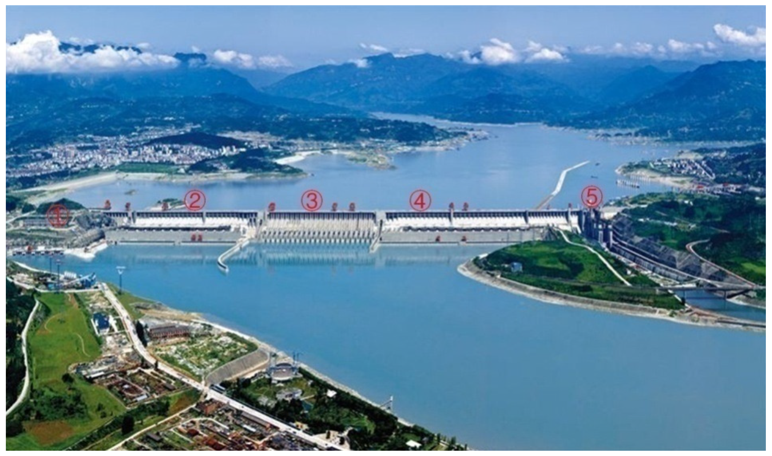
The Three Gorges Dam cross the Yangtze River in China’s Hubei Province is the largest hydroelectric project ever constructed, starting in 1994 and completed in 2009. Figure 5 shows the main component of the project, and from ① to ⑤, there are the corresponding underground powerhouse, right dam, flood discharge dam, left dam and ship lift. In this project, the underground powerhouse of this project located at the right bank of the project is inside a small mountain, named Baiyanjian, which is indicated by ① in Figure 5.

The results of the field tests for the in situ stress field demonstrated that the tectonic stress should be paid more attention than gravity stress in the underground powerhouse of the project. Before the construction of the underground powerhouse, the in situ stress field was simulated based on the measured values [10,23]. In order to verify the reasonability of the proposed approach, it is used to inversely analyze the in situ stress field; moreover, the result of the proposed approach is compared with the results of traditional approaches.

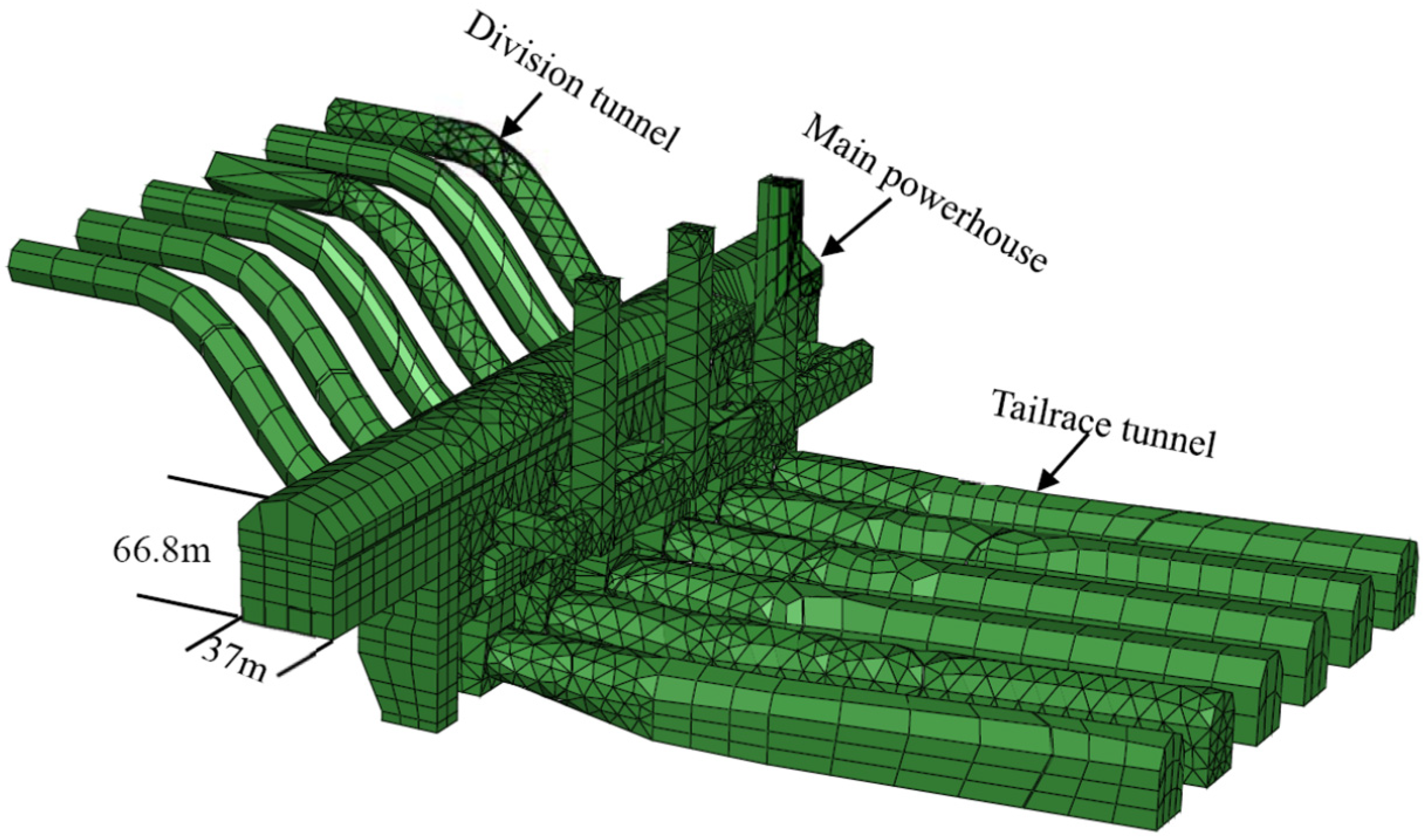
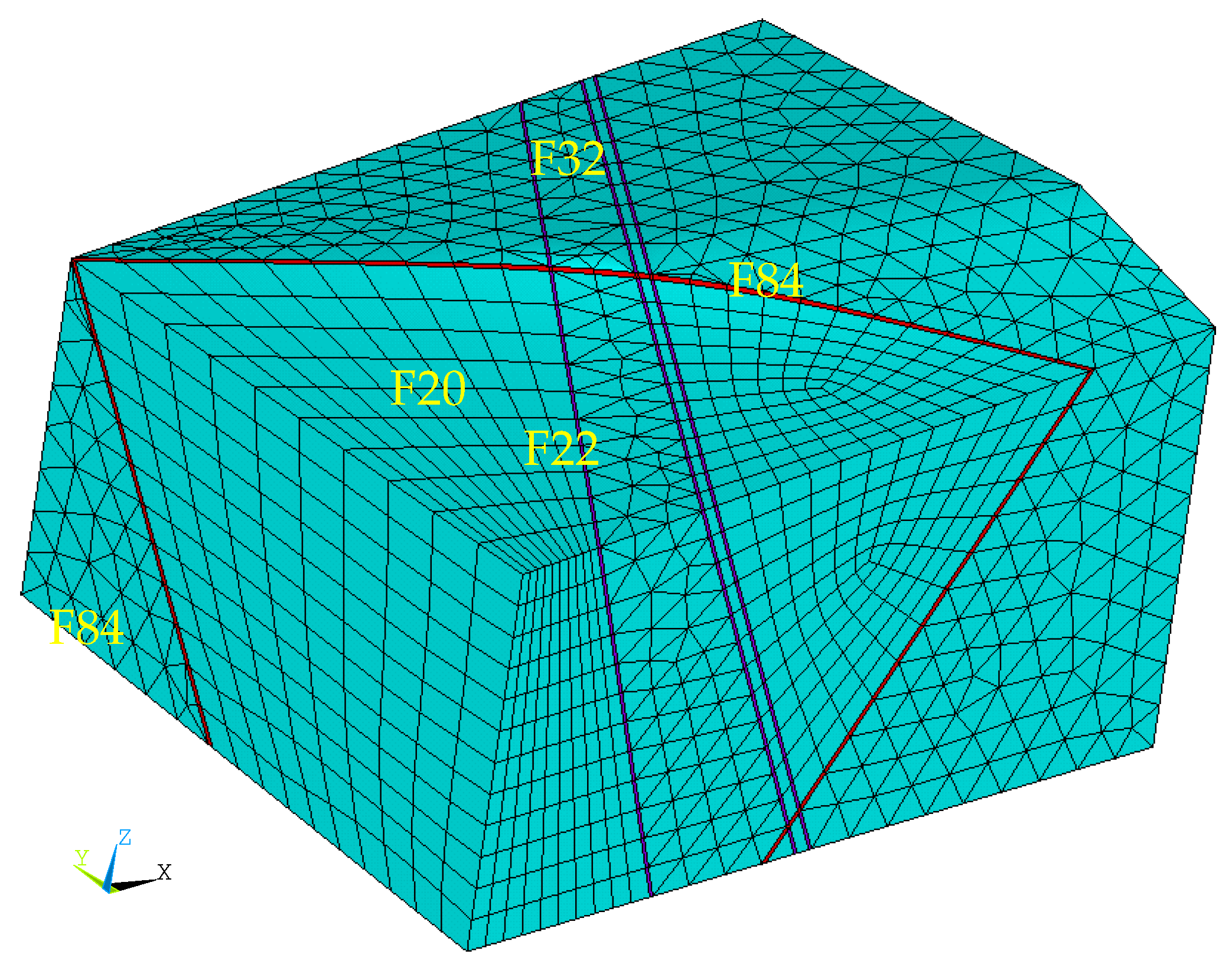
The underground powerhouse is inside a small mountain named Baiyanjian, and the top elevation of the mountain is 243 m. The underground powerhouse is 240 m long, 37 m wide, and 66.8 m high (Figure 6). The powerhouse is mainly composed of the main powerhouse, diversion tunnel, tailrace tunnel and busbar tunnel. The rock masses around the area of the underground powerhouse are mainly granite and diorite, and in this area four main faults are distributed (Figure 7); they are, respectively, named F20, F22, F32 and F84. Faults F20, F22 and F32 are filled with cataclastic rock masses, which are well cemented, and the structural planes are rough and dry. For the spatial distribution of F20, F22 and F32 with yellow color in Figure 8, the strike angle is about N240°~250° W, the dip angle is approximately 65°~70°, the extension length is greater than 300 m, and the general width is 2~5 m. For F84 (Figure 7), the fault appears as a breccia-brittle fracture zone controlled by two cross-sections, and it is sometimes wide and sometimes narrow. The fracture zone is composed of calcite caves, clusters and gaps with poor cementation and intensified weathering, and there is dripping water or flowing water along many areas of the fault. With respect to spatial distribution, the strike angle is approximately N340°~10° W, the dip angle is approximately 60°~80°, and the general width is 0.5~4 m.

According to the topography data and geologic materials of the powerhouse, the computing coordinate system and 3-D calculating model was established as in the following. The X axis is along the central line of generating units from the first to the sixth generating unit, and the Y axis is perpendicular to the axis of the powerhouse, horizontally pointing downstream. The Z axis coincides with the vertical coordinate. The origin of the coordinate system is at the intersection point between the axis of the powerhouse and the sidewall near the 1# generating unit. The scope of the coordinate system is corresponding to the following: it is [−247 573] for the X axis, [−300 400] for the Y axis, and [−250 mountaintop] for the Z axis. In this calculating model, there are 7033 nodes and 19,497 elements. Additionally, the main structural planes were considered, such as F20, F22, F32, F84. The properties of rock and main structure planes in the calculating model are shown in

Table 1. Parameters of rock mass.

Rock Mass	Weight (104 N/m3)	Young Modulus (GPa)	Poisson’s Ratio	Cohesion (MPa)	Friction Angle (°)
Slightly weathered rock mass	2.68	30	0.22	2.0	59
F20, F22, F32	2.6	15	0.25	0.20	35
F84	2.6	5	0.30	0.10	28

. These parameters were from standard tests and field tests [24].

3.2. Inverse Analysis

In order to obtain a reasonable engineering-scale in situ stress field, the stress-based approach and the proposed approach were used to simulate the engineering-scale in situ stress field. The bottom of the calculating model was fixed, and the lateral boundary conditions differed with a different approach. For the stress-based approach, the linear distribution of stress at the boundary was selected and applied on lateral boundaries during FEM calculation. For the proposed approach, the displacement boundary conditions were applied (Equations (26)–(28)) during FEM calculation. For the purpose of this study, predicting the deformation induced by excavation is not a focus, therefore, the elastic model was used during FEM computing in this paper.

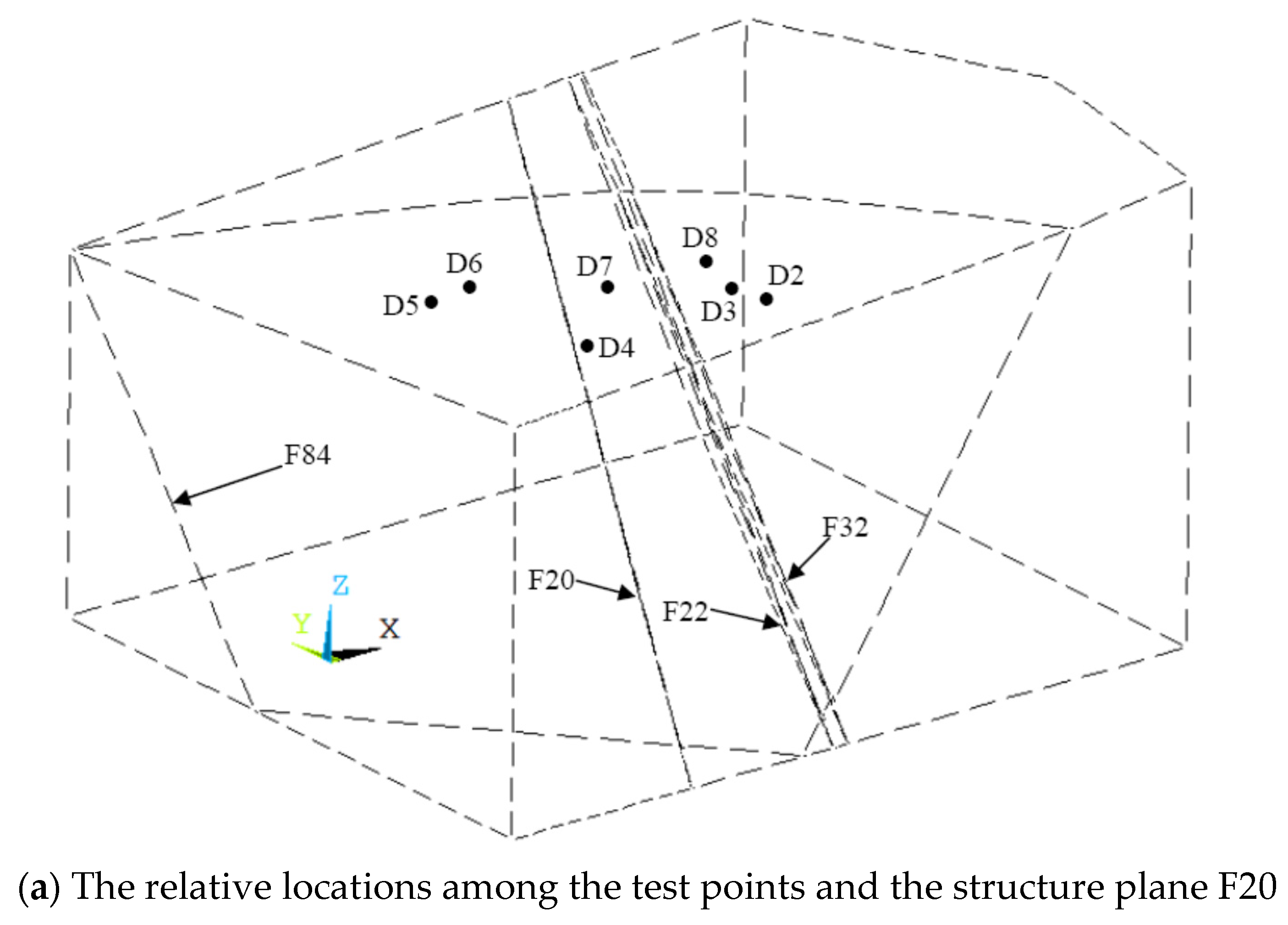
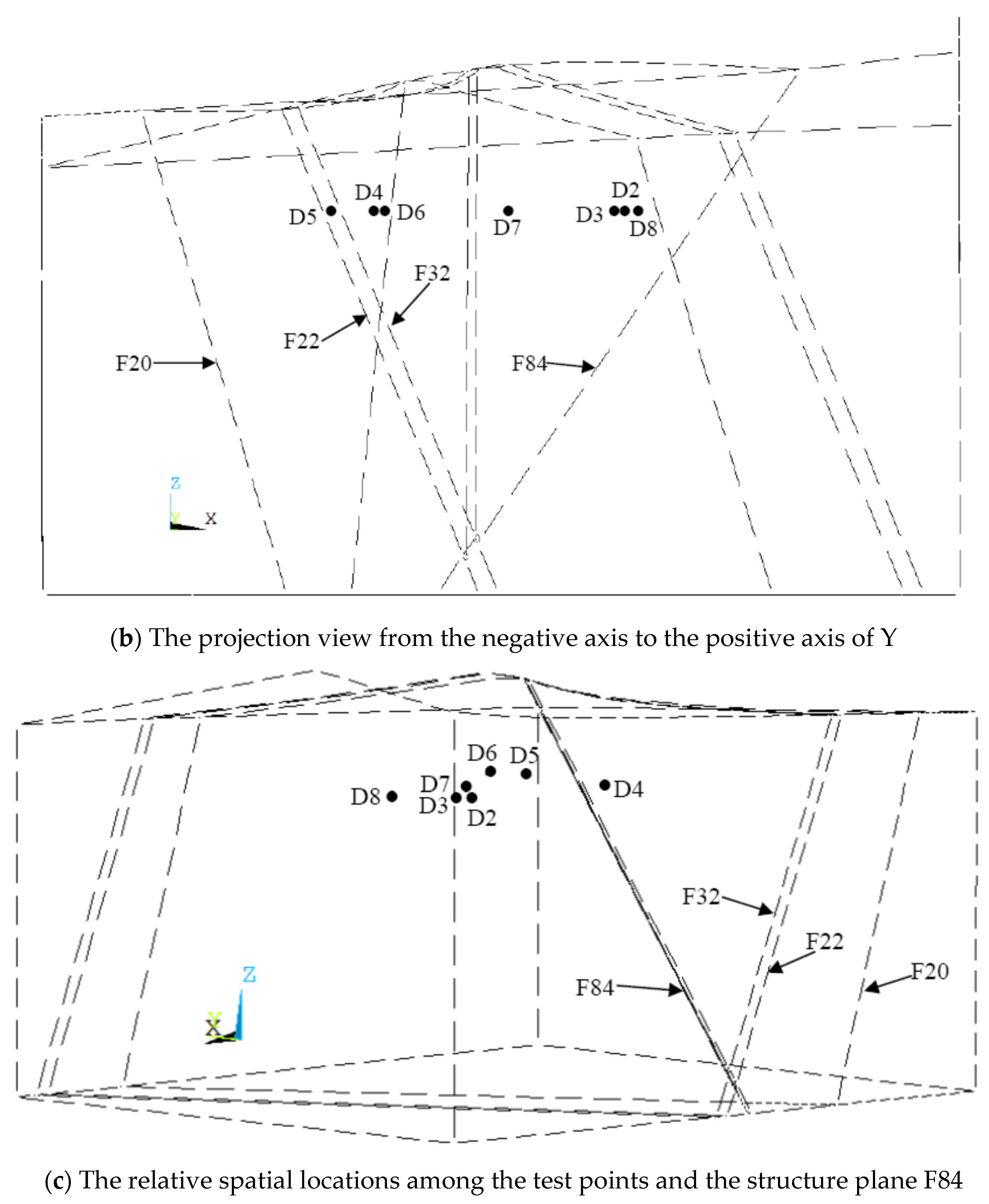
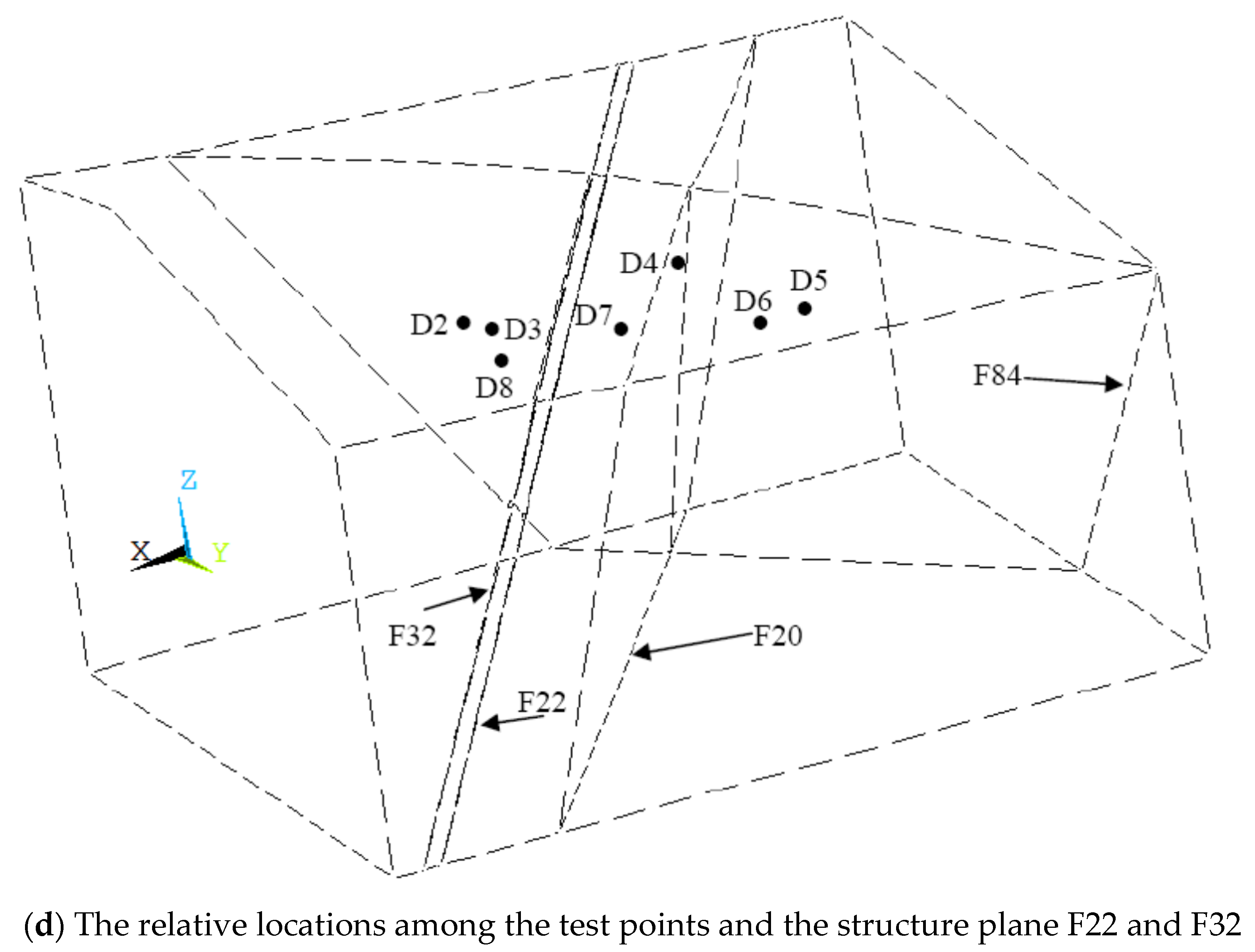
For the objective function in this project, it was established based on the measured values and corresponding calculated values (Equation (12)). The stress relief method through overcoring and hydraulic fracturing was used to test the in situ stress field (Changjiang River Scientific Research Institute, 1996). Here, the results of seven representative test points are selected as the measured values in this inverse analysis of an engineering-scale in situ stress field, which are shown in Figure 8 and

Table 2. Contrast data of stress component under calculating coordinate system.

Test Points		${\mathit{\sigma }}_{\mathit{x}}$ (MPa)	${\mathit{\sigma }}_{\mathit{y}}$ (MPa)	${\mathit{\sigma }}_{\mathit{z}}$ (MPa)	${\mathit{\sigma }}_{\mathit{x}\mathit{y}}$ (MPa)	${\mathit{\sigma }}_{\mathit{y}\mathit{z}}$ (MPa)	${\mathit{\sigma }}_{\mathit{x}\mathit{z}}$ (MPa)
D2	Measurement	−4.73	−9.06	−3.95	1.93	0.09	−0.05
	Stress based	−4.44	−9.28	−1.99	0.17	0.407	−0.058
	Strain based	−4.55	−8.98	−3.79	1.19	0.30	−0.65
D3	Measurement	−4.27	−9.47	−3.86	1.28	0.38	−0.16
	Stress based	−4.92	−8.95	−1.92	0.28	1.18	−0.165
	Strain based	−4.88	−9.52	−3.67	1.35	0.29	−0.34
D4	Measurement	−4.17	−9.13	−4.10	1.00	−0.00	−0.13
	Stress based	−4.87	−8.86	−1.83	0.24	1.11	−0.185
	Strain based	−4.59	−7.82	−2.69	1.12	0.24	−0.12
D5	Measurement	−5.46	−9.38	−5.36	1.48	0.14	−0.59
	Stress based	−4.75	−8.03	−2.23	0.27	0.65	−0.043
	Strain based	−4.86	−8.92	−3.14	1.24	−0.21	0.46
D6	Measurement	−5.52	−10.24	−5.44	1.73	−0.08	−0.31
	Stress based	−4.43	−8.54	−3.07	0.39	0.58	0.39
	Strain based	−4.71	−9.24	−2.52	1.46	−0.62	−0.10
D7	Measurement	−4.73	−8.13	−4.64	−0.23	0.01	−0.50
	Stress based	−4.44	−8.63	−3.07	0.33	0.45	0.30
	Strain based	−4.63	−8.26	−3.40	1.29	−0.20	−0.14
D8	Measurement	−4.10	−7.08	−4.42	0.53	0.20	−0.51
	Stress based	−4.33	−8.47	−2.97	0.042	1.09	0.036
	Strain based	−4.81	−9.51	−4.34	0.94	0.45	−0.55

Note: In this table, the positive sign means compression, the negative sign means tension. Stress based stands for the stress-based approach. Displacement based is on behalf of the displacement based method. Strain based means the proposed approach.

. From Figure 8, it can be seen that seven test points are sorted in order from D2 to D8, located at the same altitude, and the Z axis coordinate is 95 m (Figure 8b). The test points D4 and D7 are located between the structure planes F20 and F22 (Figure 8a), moreover, D6, D5 and D4 gradually become closer to the structure plane F84 (Figure 8c), and thus, D7, D3 and D8 are becoming gradually closely located to the structure plane F32 (Figure 8a,d), and D6, D7 and D4 are gradually close to the structure plane F20 (Figure 8a). In the proposed approach, only six strain variables need to be optimized, and therefore, the simplex optimization algorithm was adopted in this paper. This simplex optimization algorithm in the MATLAB software can be used and the optimizing process was implemented using the MATLAB code combining the simplex optimization algorithm and the in situ stress calculation with FEM.

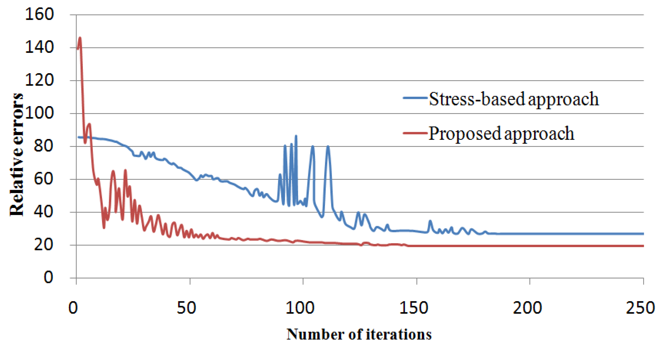
The optimization processes with both approaches are shown in Figure 9. It can be seen that the proposed approach has faster convergence and a better convergence process than the stress-based approach. It also shows that the simplex optimization algorithm is sufficient.

3.3. Results of Engineering-Scale In Situ Stress

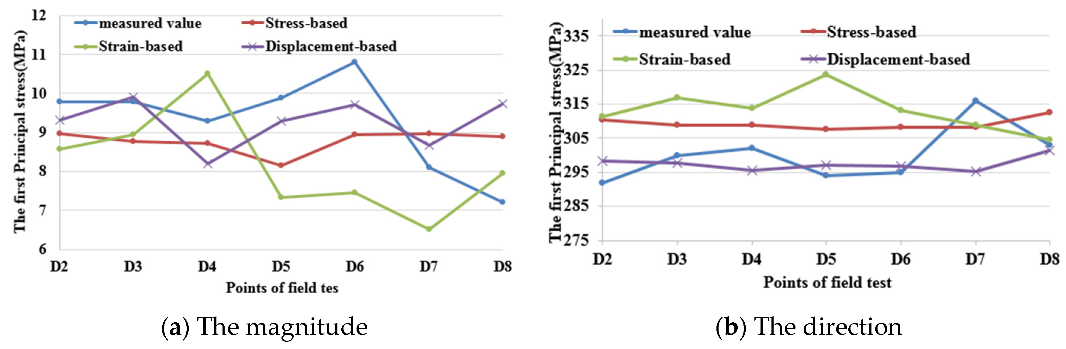
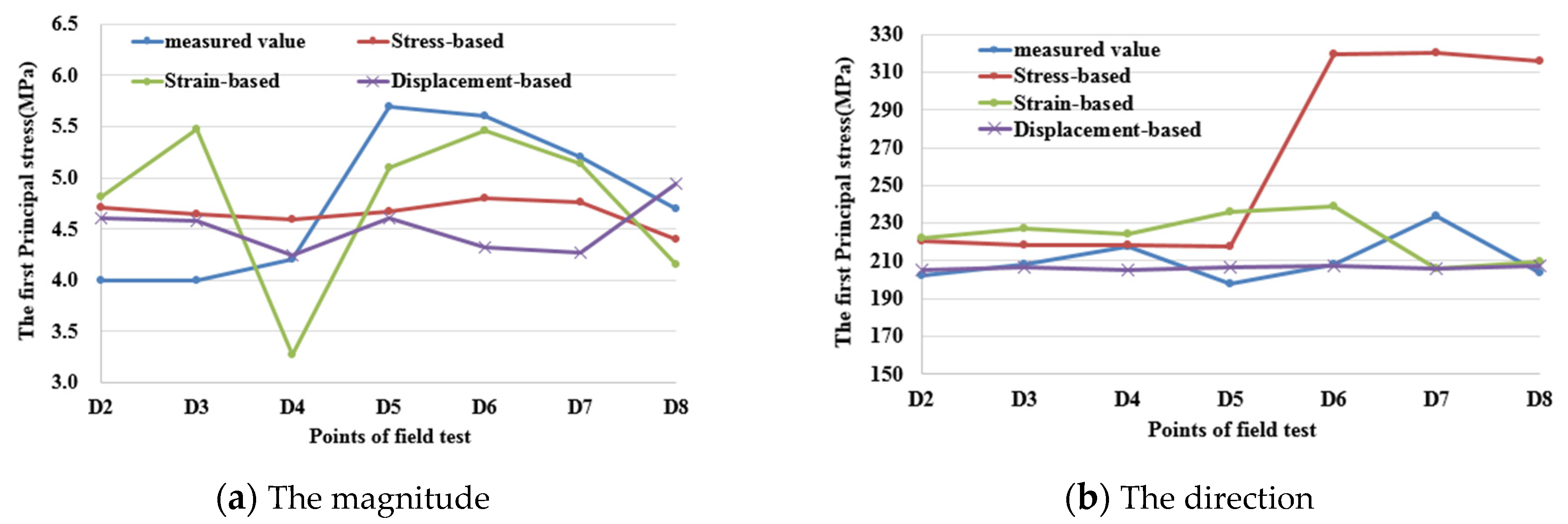
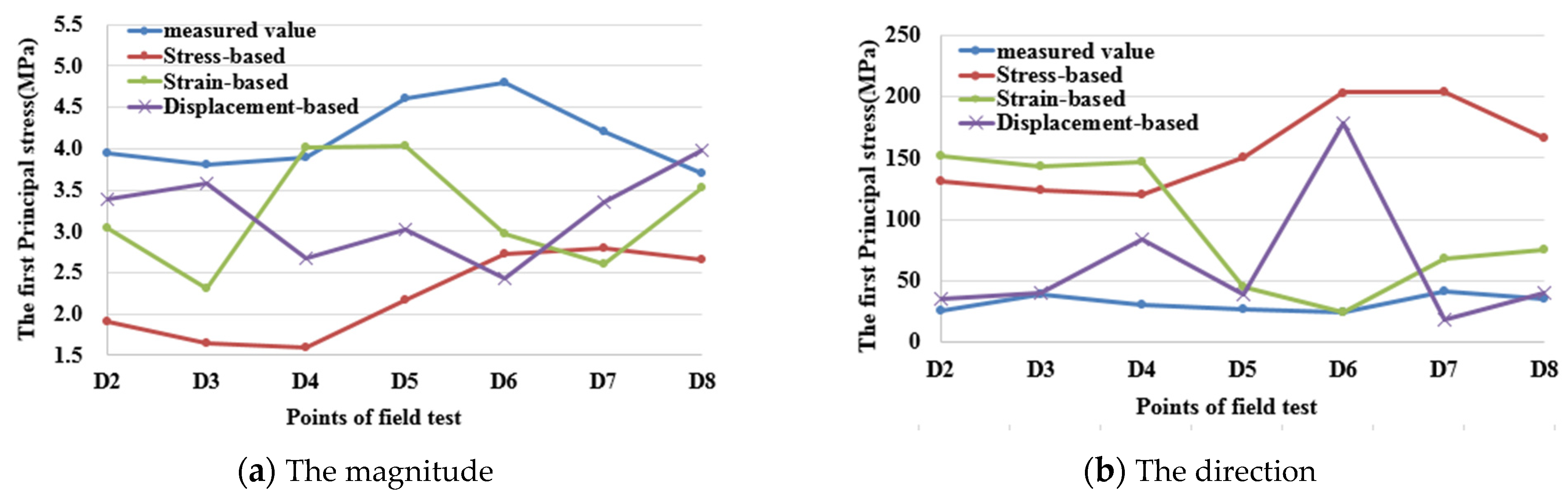
Figure 10, Figure 11 and Figure 12 show the comparison between the measured and calculated values of in situ stress at test points, where the red curve refers to the measured value, the blue curve stands for the calculated value with the stress-based approach, the green curve is for the calculated value using the proposed method, and the gray color means the results with the displacement-based approach. The calculating results using the displacement-based approach were from the previous work [10], and the displacement mode was assumed as the linear displacement when the in situ stress in the region of interest was inversely analyzed. Figure 10 shows the comparison by different approaches for the magnitude and direction of the first principal stress. Similarly, Figure 11 is for the second principal stress, and Figure 12 is for the least principal stress.

From the comparison, it can be seen that for the magnitude of principal stress, the calculated values with the proposed approach have better agreement with the measured values than those by the stress-based approach and displacement-based approach. For the stress-based approach, the magnitudes of principal stress differ significantly with the measured values in some test points, especially with respect to the least principal stress. For the displacement-based approach, there are obvious differences among the calculated values at points D4, D6, D7 and the corresponding measured values, which may be caused by the spatial locations of these points close to the faults (Figure 8). For the proposed approach, in the first principal stress, there are significant differences for the comparison between the calculated and the measured value at points D4 and D7. However, in the second principal stress, the obvious difference of the comparison appears at points D6 and D7, and for the least principal stress, the calculated values are obviously inconsistent with the measured values at points D4 and D6. Therefore, some conclusion can be drawn that the main fault has important influence on the inverse calculating results of the in situ stress. For the underground powerhouse of the Three Gorges project, because points D4, D6, and D7 are close to faults F84, F20 and F22, and the calculated results by any approach are significantly different than the measured value at these points. For these approaches, the stress-based approach is worse than others. Though the displacement-based approach is popular, the relative error using this method cannot be ignored. For the proposed method, better estimation for in situ stress can be obtained through comparisons with other approaches.

Table 2 and

Table 3. Contrast data of principal stress under geodetic coordinate system.

Test Points		${\mathit{\sigma }}_{\mathbf{1}}$ (MPa)	Azimuth (°)	Inclination (°)	${\mathit{\sigma }}_{\mathbf{2}}$ (MPa)	Azimuth (°)	Inclination (°)	${\mathit{\sigma }}_{\mathbf{3}}$ (MPa)	Azimuth (°)	Inclination (°)
D2	Measurement	9.80	292.00	1.00	4.00	202.00	15.00	3.94	26.00	75.00
	Stress based	8.98	310.44	3.72	4.71	220.5	0.062	1.91	131.4	86.2
	Displacement based	8.58	311.36	12.77	4.82	222.40	4.69	3.04	152.20	76.35
	Stain based	9.32	298.33	4.73	4.60	205.29	32.69	3.39	35.62	56.88
D3	Measurement	9.80	300.00	4.00	4.00	208.00	23.00	3.80	39.00	67.00
	Stress based	8.78	308.7	11.02	4.65	218.5	0.81	1.64	124.3	78.9
	Displacement based	8.95	316.89	9.89	5.48	227.06	0.977	2.31	142.65	80.06
	Stain based	9.91	297.73	3.36	4.58	206.82	15.24	3.58	39.85	74.38
D4	Measurement	9.30	302.00	4.00	4.20	218.00	60.00	3.90	30.00	30.00
	Stress based	8.72	308.7	10.5	4.59	218.5	1.52	1.59	120.4	79.3
	Displacement based	10.50	313.75	6.35	3.27	223.91	1.49	4.02	147.13	83.48
	Stain based	8.19	295.62	2.79	4.24	205.53	1.72	2.68	83.90	86.72
D5	Measurement	9.90	294.00	4.00	5.70	198.00	55.00	4.60	27.00	35.00
	Stress based	8.16	307.6	6.68	4.67	217.9	2.81	2.17	150.6	82.7
	Displacement based	7.32	323.60	4.42	5.10	235.90	27.62	4.04	45.26	61.90
	Stain based	9.28	297.09	3.07	4.61	206.30	14.34	3.02	38.89	75.32
D6	Measurement	10.80	295.00	2.00	5.60	208.00	64.00	4.80	24.00	26.00
	Stress based	8.95	308.2	5.26	4.80	319.5	18.5	2.72	203.2	70.7
	Displacement based	7.46	313.13	18.12	5.46	239.13	40.09	2.97	24.40	44.30
	Stain based	9.71	296.87	4.53	4.32	207.54	8.39	2.43	178.81	80.45
D7	Measurement	8.10	316.00	6.00	5.20	234.00	43.00	4.20	41.00	45.00
	Stress based	8.97	308.3	4.13	4.76	320.5	15.8	2.79	204.06	73.65
	Displacement based	6.51	308.80	21.20	5.14	205.80	30.00	2.61	68.50	51.80
	Stain based	8.68	295.35	1.60	4.27	205.70	12.61	3.35	18.24	77.29
D8	Measurement	7.20	303.00	7.00	4.70	204.00	56.00	3.70	35.00	34.00
	Stress based	8.89	312.5	10.82	4.40	316.13	7.17	2.65	166.7	76.97
	Displacement based	7.95	304.5	16.19	4.15	209.30	17.19	3.52	75.30	66.01
	Stain based	9.75	301.56	5.85	4.94	207.55	34.27	3.98	40.00	55.09

also showed the comparison among different approaches. In both tables, the positive sign means compression, and the negative sign means tension. Additionally, in

Table 4. The statistical relative errors between inversion results and measurement values.

Method	${\mathit{\sigma }}_{\mathbf{1}}$ (%)	Azimuth (%)	Inclination (%)	${\mathit{\sigma }}_{\mathbf{2}}$ (%)	Azimuth (%)	Inclination (%)	${\mathit{\sigma }}_{\mathbf{3}}$ (%)	Azimuth (%)	Inclination (%)
Stress based	3.64	3.03	123.34	0.56	24.29	87.14	46.53	414.84	99.33
Displacement based	10.6	4.37	369.16	1.35	6.66	64.10	21.71	199.01	65.15
Strain based	1.50	0.86	48.61	3.47	1.58	40.46	21.06	123.81	90.62

, the calculating results are also shown using the stress-based approach. In both tables, stress-based stands for the stress-based approach, displacement-based represents the displacement-based approach, strain-based is on behalf of the proposed approach, and the measurement means the measured value in field tests. From the comparison of data in both tables, for the principal stresses, the same conclusion can be obtained as those from the above Figure 10, Figure 11 and Figure 12.

Table 4 reveals the corresponding statistical relative errors between the calculating principal stresses by the stress-based approach, displacement-based approach, the proposed approach and the measurement values. Here, for each measurement point, the relative error is the percentage between the absolute error and the measurement value (Equation (30)). In Table 4, the relative error is the mean of the relative errors of all measurement points [25]. Therefore, it can be concluded that the proposed approach in this paper is more effective than the traditional approach in determining the engineering-scale in situ stress field:

$${\mathit{E}}_{\mathit{r}}=\frac{{\mathit{E}}_{\mathit{a}}}{\mathit{T}}=\frac{\Vert X-\mathit{T}\Vert }{\mathit{T}}$$

(30)

where E_r is the relative error, E_a is the absolute error, X is the inversion value by different approach, T is the measurement value at each point.

4. Conclusions

(1) Based on engineering-scale tectonic strain, a new inverse analysis approach is proposed for the engineering-scale in situ stress field. In contrast to traditional stress-based and displacement-based approaches, this approach overcomes the drawbacks of boundary mode selection in traditional methods. This therefore avoids the ambiguity of inconsistent in situ stresses resulting from the different boundary modes that are chosen.

(2) In the proposed approach, there are only six variables that need to be optimized, which overcomes the challenge of high dimensionality optimization in traditional approach. Furthermore, the six variables in the proposed approach stand for tectonic strain on boundary, which have physical meaning.

(3) The proposed approach is applied in the determination of the engineering-scale in situ stress of underground powerhouse of the Three Gorges Project. The results by the proposed approach are compared with the measured values in field tests and the results by stress-based and displacement-based approaches. The comparison demonstrates that the calculated values with the proposed approach have better agreement with the measured values than those by stress-based approach and displacement-based approach.

References

- Konietzky, H.; Te Kamp, L.; Hammer, H.; Niedermeyer, S. Numerical modeling of in situ stress conditions as an aid in route selection for railtunnels in complex geological formations in South Germany. Comput. Geotech. 2001, 28, 495–516. [Google Scholar] [CrossRef]
- McKinnon, S.D. Analysis of stress measurements using an umerical model methodology. Int. J. Rock Mech. Min. Sci. 2001, 38, 699–709. [Google Scholar] [CrossRef]
- Deng, J.H.; Lee, C.F. Displacement back analysis for a steep slope at the Three Gorges Project site. Int. J. Rock Mech. Min. Sci. 2001, 38, 259–268. [Google Scholar] [CrossRef]
- Chen, Y.F.; Zheng, H.K.; Wang, M.; Hong, J.M.; Zhou, C.B. Excavation-induced relaxation effects and hydraulic conductivity variations in the surrounding rocks of a large-scale underground powerhouse cavern system. Tunn. Undergr. Space Technol. 2015, 49, 253–267. [Google Scholar] [CrossRef]
- Hong, J.M.; Chen, Y.F.; Liu, M.M.; Zhou, C.B. Inverse modelling of groundwater flow around a large-scale underground cavern system considering the excavation-induced hydraulic conductivityvariation. Comput. Geotech. 2017, 81, 346–359. [Google Scholar] [CrossRef]
- Ito, T.; Igarashi, A.; Kato, H.; Ito, H.; Sano, O. Crucial effect of system compliance on the maximum stress estimation in the hydrofracturing method: Theoretical considerations and field-test verification. Earth Planets Space 2006, 58, 963–971. [Google Scholar] [CrossRef] [Green Version]
- Liu, Y.; Li, H.; Luo, C.; Wang, X. In situ stress measurements by hydraulic fracturing in the western route of south to north water transfer project in China. Eng. Geol. 2014, 168, 114–119. [Google Scholar] [CrossRef]
- Xu, R. The GA-ANN method for determiningcalculation parameters for deep excavation. J. Zhejiang Univ. Sci. 2000, 1, 408–413. [Google Scholar]
- Zhang, L.Q.; Yue, Z.Q.; Yang, Z.F.; Qi, J.X.; Liu, F.C. A displacementbasedback-analysis method for rock mass modulus andhorizontal in situ stress in tunneling–illustrated with acase study. Tunn. Undergr. Space Technol. 2006, 21, 636–649. [Google Scholar] [CrossRef]
- Guo, M.W.; Li, C.G.; Wang, S.L.; Luan, G.B. Study oninverse analysis of 3-D initial geostress field withoptimized displacement boundaries. Rock Soil Mech. 2008, 29, 1269–1274. (In Chinese) [Google Scholar]
- Li, Y.; Yin, J.; Chen, J.; Xu, J. Analysis of 3D in-situstress field and query system’s development basedon visual BP neural network. Procedia Earth Planet. Sci. 2012, 5, 64–69. [Google Scholar]
- Zhang, S.; Yin, S. Determination of in situ stresses and elastic parameters from hydraulic fracturing tests by geomechanics modeling and soft computing. J. Pet. Sci. Eng. 2014, 124, 484–492. [Google Scholar] [CrossRef]
- Singh, U.K.; Sahoo, B.C. Computing the 3D in-situ stress field from shut-in pressure data using statistical regression. Geotech. Geol. Eng. 2000, 18, 119–137. [Google Scholar] [CrossRef]
- Yu, J.H.; Jin, W.L.; Zou, D.Q. Displacementfunction method for analyzing initial earth stress. Rockand Soil Mech. 2003, 24, 417–419. (In Chinese) [Google Scholar]
- Yue, X.; Li, Y.; Wang, H. Inversion of initial in-situ stress fieldby the method of multivariate analysis and engineering application. Appl. Mech. Mater. 2011, 44–47, 1203–1206. [Google Scholar]
- Zhang, S.R.; Hu, A.K.; Wang, C. Three-dimensional inversion analysis of an in situ stress field based on a two-stage optimization algorithm. J. Zhejiang Univ. Sci. A 2016, 17, 782–802. [Google Scholar] [CrossRef] [Green Version]
- Li, F.; Wang, J.A.; Brigham, J.C. Inverse calculation of in-situ stressin rock mass using the Surrogate-Model Accelerated RandomSearch algorithm. Comput. Geotech. 2014, 61, 24–32. [Google Scholar] [CrossRef]
- Koch, P.N.; Simpson, T.W.; Allen, J.K.; Mistree, F. Statistical approximations for multidisciplinary design optimization: The problem of size. J. Aircr. 1999, 36, 275–286. [Google Scholar] [CrossRef]
- Li, B.; Li, Y.; Zhu, W.; Li, C.; Dong, Z. Impact of in-situ stress distribution characteristics on jointed surrounding rock mass stability of an underground cavern near a hillslope surface. Shock Vib. 2017, 2017, 2490431. [Google Scholar] [CrossRef]
- Zhu, W.; Li, Y.; Li, S.; Wang, S.; Zhang, Q. Quasi-three-dimensional physical model tests on a cavern complex under high in-situ stresses. Int. J. Rock Mech. Min. Sci. 2011, 48, 199–209. [Google Scholar]
- Li, F. Numerical simulation of 3D in-situ stress in Hailaer oil field. Procedia Environ. Sci. 2011, 12, 273–279. [Google Scholar] [CrossRef] [Green Version]
- Fu, C.; Wang, W.; Chen, S. Back analysis study on initial geostress field of dam site for Xiluodu hydropower project. Chin. J. Rock Mech. Eng. 2006, 11, 2305–2312. (In Chinese) [Google Scholar]
- Zhong, Z.; Gong, B.; Lv, G. Measurement and research of in-situ stress field in the zone of underground powerhouse of the Three Gorges Project. J. Yangtze River Sci. Res. Inst. 1996, 13, 17–19. [Google Scholar]
- Changjiang River Scientific Research Institute. Report of In-Situ Stress Measurement for the Underground Powerhouse of the Three Gorges Project; Changjiang River Scientific Research Institute: Wuhan, China, 1996. [Google Scholar]
- Cuomo, S.; Moscariello, M.; Manzanal, D.; Pastor, M.; Foresta, V. Modelling the mechanical behaviour of a natural unsaturated pyroclastic soil within generalized plasticity framework. Comput. Geotech. 2018, 99, 191–202. [Google Scholar] [CrossRef]
Figure 1.
Sketch of 3-D calculating model.
Figure 2.
Sketch of normal and shear stress boundary.
Figure 3.
Sketch of displacements on boundaries ABEF and BCDE.
Figure 4.
Calculating process of the proposed method.
Figure 5.
Overall view of the Three Gorges Project.
Figure 6.
Main caverns of underground powerhouse.
Figure 7.
3D FEM calculating model.
Figure 8.
The spatial distribution of seven test points in 3D calculating model.
Figure 9.
Optimization processes using the stress-based and proposed approaches.
Figure 10.
Comparison with measured values of the first principal stress.
Figure 11.
Comparison with measured values of the second principal stress.
Figure 12.
Comparison with measured values of the least principal stress.