Mean Dynamic Topography Modeling Based on Optimal Interpolation from Satellite Gravimetry and Altimetry Data

Abstract

Mean dynamic topography (MDT) is crucial for research in oceanography and climatology. The optimal interpolation method (OIM) is applied to MDT modeling, where the error variance–covariance information of the observations is established. The global geopotential model (GGM) derived from GOCE (Gravity Field and Steady-State Ocean Circulation Explorer) gravity data and the mean sea surface model derived from satellite altimetry data are combined to construct MDT. Numerical experiments in the Kuroshio over Japan show that the use of recently released GOCE-derived GGM derives a better MDT compared to the previous models. The MDT solution computed based on the sixth-generation model illustrates a lower level of root mean square error (77.0 mm) compared with the ocean reanalysis data, which is 2.4 mm (5.4 mm) smaller than that derived from the fifth-generation (fourth-generation) model. This illustrates that the accumulation of GOCE data and updated data preprocessing methods can be beneficial for MDT recovery. Moreover, the results show that the OIM outperforms the Gaussian filtering approach, where the geostrophic velocity derived from the OIM method has a smaller misfit against the buoy data, by a magnitude of 10 mm/s (17 mm/s) when the zonal (meridional) component is validated. This is mainly due to the error information of input data being used in the optimal interpolation method, which may obtain more reasonable weights of observations than the Gaussian filtering method.

1. Introduction

Mean dynamic topography (MDT) is the deviation between the mean sea surface (MSS) and the geoid, which plays an important role in disciplines like oceanography and climatology. In the field of geodesy, an accurate MDT is necessary for the unification of the land–sea vertical datum and research on the Earth’s rotation [1,2]. In addition, in the field of oceanography, the parameters of MDT are of great importance in the study of ocean circulation, sea-level change, and energy transport mechanisms in the ocean. The ocean circulation derived from the MDT can be applied to monitor the movement of pollutants, which is of great significance for marine environmental monitoring [3]. Moreover, the ocean current system promotes the energy exchange between the high and low latitudes of the earth, which in turn affects global climate change. The stability and variability of ocean circulation and its related transfer of extreme heat and freshwater can have a significant impact on local and even global climate change. For example, the Kuroshio warm current and the Oyashio cold current have important impacts on the weather and climate of China and Japan; the Gulf Stream has an important impact on the climate of North America and Europe; and the changes in ocean currents in the equatorial Pacific and El Niño and La Niña are also closely related to the global climate characteristics.

Based on the geodetic approach, the MSS and the geoid can be obtained by satellite altimetry technology and the gravity geopotential model (GGM), respectively [4], while the difference between them is the MDT. However, limited by the observation technique, the GGM would contribute to a higher level of errors than the MSS in solving the MDT [5]. In recent years, with the development of gravity satellites, especially the successive launch of the Gravity Recovery and Climate Experiment mission (GRACE), the Gravity Field and Steady-State Ocean Circulation Explorer mission (GOCE), and the GRACE Follow-On mission, the accuracy and resolution of GGM have been significantly improved [6,7,8]. These dedicated satellite missions facilitate many applications in earth science, including understanding ocean circulations in oceanography and studying tectonic–geodynamic activities [9]. Currently, the highest degree and order (d/o) of the satellite-only GGM can be up to 300 d/o, corresponding to a spatial resolution of about 66 km [10].

However, the spatial resolution of MSS can currently reach 1′ (~10 km), which is much higher than that of the GGM [11]. As a result, because of the spectral inconsistency, it will cause problems such as spectral aliasing and spectral leakage when removing the geoid signal directly from the MSS [5]. Accordingly, a filtering procedure is mandatory to unify the spectrum between the MSS and the geoid. Researchers now have investigated different filtering methods for reasonable MDT solutions, such as Gaussian filtering and wavelet filtering [12,13,14]. The weighting scheme of Gaussian filtering is usually only related to distance, which may not be the best method. In addition, Vianna et al. [15] developed an adaptive filtering method based on singular spectrum analysis to solve high-resolution MDT. This method is adequate for the finite domain MDT processing since it minimizes smoothing and does not lose boundary points. The signal and noise can effectively separate by this method. But these filtering methods still lead to signal leakage and distortion problems, and it is difficult to give the error distribution of the MDT model. Compared with the previous studies, Rio et al. [5,16] introduced an optimal interpolation method (OIM) in a combination of the MSS and GGM, which considered the covariance between observations. The estimated MDT can be smoothed while preserving more detailed signals, which mitigates the problems of signal leakage or distortion, and error information of the MDT is estimated. The key point of the OIM focuses on the construction of the covariance function, involving the estimation of the parameters like the variance of the MDT and the correlation radius.

The accurate information of the MSS and especially the GGM has a direct influence on the MDT reconstruction. In fact, the GOCE mission now can detect more accurate gravity signals thanks to the equipment of the gradient gravimeter in the GOCE gravity satellite. Specifically, the European Space Agency (ESA) has released six generations of GGM based on GOCE gravity data and direct approach; the fourth-generation model (GO_CONS_GCF_2_DIR_R4, DIRR4) assimilated data from 2009 to 2012, and the fifth-generation model (GO_CONS_GCF_2_DIR_R5, DIRR5) and the sixth-generation model (GO_CONS_GCF_2_DIR_R6, DIRR6) used all the data from 2009 to 2013. In addition, the DIRR6 recalibrated the satellite’s orbits compared to the DIRR5 [17]. The influence of these differences between GGMs on the constructed MDTs can be further investigated. In addition, the recently released DTU18 MSS incorporates the latest satellite altimetry data, especially Jason, CyroSat-2, and SARAL/Altika, which is expected to further improve the accuracy of the MSS.

The aim of this study includes three aspects. First, we quantify the effects on MDT recovery based on the recently released GOCE-derived GGMs, which are expected to further improve the MDT modeling in terms of spatial resolution and accuracy. In addition, the choice of MSS is studied, in which the recently published MSS models are compared to see if the choice of MSS has nonignorable effects on MDT modeling. Then, we compare the performances of the traditionally used Gaussian filtering method with the optimal interpolation approach, providing an insight with respect to the choice of approach in MDT recovery.

The structure of this study is as follows: In Section 2, the main principle of the OIM in MDT modeling is briefly introduced. Then, the estimation of the key parameters in the OIM is introduced. Numerical experiments are shown in Section 3, in which the Kuroshio is selected as the research area, and the oceanographic and geodetic MDTs and the buoy-measured ocean geostrophic current-velocity profiles are used for comparison and validation. The summary of this study and a brief conclusion are given in Section 4.

2. Data and Methods

2.1. Study Area and Data

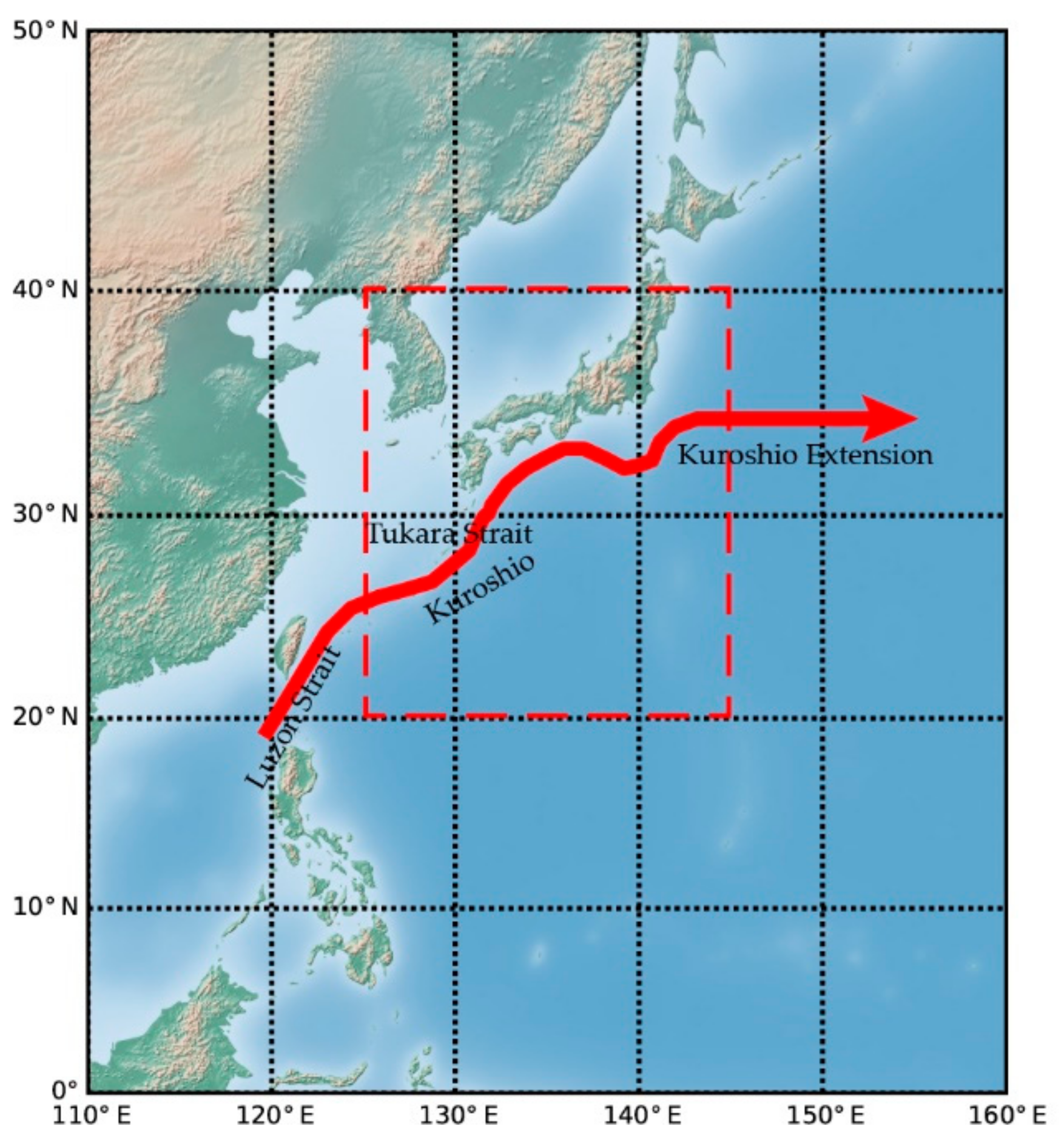
The study area was located in a part of the Kuroshio current (20–40° N, 125–145° E), which is shown in Figure 1 (image adapted from Shaded Relief, http://www.shadedrelief.com/ (accessed on 15 March 2021)). The Kuroshio current is the western boundary in the wind-driven, subtropical, and subarctic circulations of the North Pacific Ocean. The Kuroshio brings the high temperature and high salinity seawater of the equatorial Pacific Ocean to the vast offshore sea areas, which has a huge impact on the ocean, meteorology, and hydrology of these areas. Moreover, the Kuroshio also transports a large amount of heat from the low latitudes of the North Pacific to the middle and high latitudes, so its seasonal and interannual changes have an important impact on the climate and environment of neighboring countries and even the world [5,18]. There is important scientific significance in studying the MDT and geostrophic current in this area.

2.1.1. Mean Sea-Surface Model

The mean sea-surface model is a key element for modeling MDT. DTU15 MSS and DTU18 MSS, published by the Danish Technical University (DTU), were chosen to construct MDT in the paper. DTU15 MSS uses the last 4 years of Cryosat-2 data to improve the accuracy of the MSS model. The resolution of DTU15 MSS is 1′ × 1′. DTU18 MSS is based on the previous generation model DTU15 MSS, incorporating 3 years of Sentinel-3A and 7 years of Cryosat-2 altimetry data from two satellites that provide data in SAR mode, and using the new tide model FES2014, which allows for a more accurate MSS [11]. DTU18 MSS has a spatial resolution of 1′ × 1′ and a reference time of 1993–2012.

2.1.2. Global Geopotential Models

In order to facilitate the estimation of errors of the geoid, this study introduces multigeneration, GOCE-derived GGMs solved by the direct and time-wise approaches: the GO_CONS_GCF_2_DIR_R4 (DIRR4), GO_CONS_GCF_2_DIR_R5 (DIRR5), and GO_CONS_GCF_2_DIR_R6 (DIRR6); and the GO_CONS_GCF_2_TIM_R4 (TIMR4), GO_CONS_GCF_2_TIM_R5 (TIMR5), and GO_CONS_GCF_2_TIM_R6 (TIMR6) [9,19].

Table 1. Summary of the multigeneration GOCE-derived GGMs.

Geoid Model	Maximum d/o	Assimilated GOCE Data
DIRR4	260	Nov. 2009–Aug. 2012
DIRR5	300	Nov. 2009–Oct. 2013
DIRR6	300	Oct. 2009–Oct. 2013
TIMR4	250	Nov. 2009–Jun. 2012
TIMR5	280	Nov. 2009–Oct. 2013
TIMR6	300	Oct. 2009–Oct. 2013

summarizes detailed information about these GOCE-derived GGMs. Figure 2 shows the error-degree variance in geoid height calculated by different GOCE-derived GGMs. It shows that the period of the assimilated data was extended with the development of the generation, and the supplement of data improved the modeling accuracy. The accuracy of the direct solution model was higher than that of the time domain solution model. With the update of the GOCE gravity data and the update of the solution method, the error of the time domain solution model showed a significant downward trend, while in the direct solution model, the accuracy of DIRR5 was higher than that of DIRR4, but the accuracy of DIRR6 was higher than DIRR5 before order 170, and lower than DIRR5 when the order was greater than 170. This may be due to the parameters set in the solution of these two models. While different from the data used, this result did not mean that the accuracy of DIRR6 was lower than DIRR5. Regarding the error of the GOCE satellite gravity field model, ESA has issued a related report that used externally measured GPS/leveling data to evaluate the accuracy of the multigeneration gravity field model. The results showed that the accuracy of the DIRR6 was better than that of the DIRR5 [20].

2.1.3. Ocean Numerical Models and Reference MDT

In order to make the comparison between the MDT solutions and the empirical MDTs, several ocean numerical models; i.e., Simple Ocean Data Assimilation 3 (SODA3), Ocean and Sea-Ice Reanalysis System (ORAS5), Copernicus, and geodetic model CNES-CLS13MDT were used in this study. The spatial resolutions of the SODA3, ORAS5, and Copernicus ocean models were all 1/4°, but the reference time of these MDTs was different; detailed information is listed in

Table 2. Details of the ocean numerical models.

Ocean Numerical Model	Spatial Resolution	Time Scale	References
SODA3	1/4°	1980–2017	Carton et al. [22]
ORAS5	1/4°	1979–2018	Zuo et al. [23]
Copernicus	1/4°	1993–2019	Product User Guide [24]
CNES-CLS13MDT	1/4°	1993–2012	Rio et al. [25]

. Based on Sea Level Anomalies (SLA) data provided by Aviso (ftp://ftp-access.aviso.altimetry.fr/climatology (accessed on 19 May 2020)), the reference time of these MDTs was unified to the same time period [21].

2.1.4. Drifting-Buoy Data

In situ ocean buoy data can be used to compare and verify MDT, because the geostrophic ocean current velocities can be extracted from buoy data and derived from MDT. The buoy data were obtained from the Global Drifter Program (GDP) provided by the U.S. National Oceanic and Atmospheric Administration (NOAA) and the Atlantic Ocean and Meteorological Laboratory (AOML), and they have been quality-controlled and kriged in order to provide 6-hour velocity measurements. The GDP uses satellite-tracked drifting buoys on the ocean surface to obtain current velocity, temperature, and salinity data. This study used buoy data from 1993–2016, and the buoys’ observed current parameters included geostrophic, tidal, Ekman, inertial, and high-frequency nongeostrophic currents. Since only the geostrophic ocean current could be deduced by the MDT, the buoy observations needed to be processed to remove the nongeostrophic component. The Ekman component can be modeled based on the data of the wind speed and wind stress. Thus, the Ekman current model developed by Rio [16] was used to remove the Ekman current from the buoy data, and a 3-day low-pass filter was applied to the residual buoy current to remove tidal, inertial, and high-frequency nongeostrophic components [26,27]. The mean zonal and meridional geostrophic velocities were finally averaged into 1/4° grids. Moreover, to evaluate the accuracy of the geostrophic velocities, the errors of this data set was estimated, which can be given as the standard deviation of the observations divided by the square root of the number of observations [5]. The statistics of the errors are shown in

Table 3. Statistics of the errors of the drifter geostrophic velocity (units: mm/s).

Geostrophic Velocity	Max	Mean	RMS
Zonal component	823	4.2	14.3
Meridional component	445.8	6.9	11.9

. It shows that the RMS (root mean square) of the errors of the zonal (meridional) drifter geostrophic velocity were 14.3 mm/s (11.9 mm/s), respectively.

2.2. Optimal Interpolation Method

The MDT is expressed by the difference between the MSS and geoid, which is given by:

$$\mathrm{h}=\overline{\mathsf{\eta }} - \mathrm{N}$$

(1)

with the MDT $\mathrm{h}$, the MSS $\overline{\mathsf{\eta }}$, and the geoid $\mathrm{N}$, which should be combined under the same coordinate system and tide system. Considering the GOCE-derived GGM and the MSS models used in this study, the models were transformed to the GRS80 and zero-tide system.

In order to mitigate the signal distortion and leakage problems induced by the traditional filtering methods, this study adopted the OIM (also known as multivariate objective analysis) for the MDT modeling, which was first applied to oceanographic parameter estimation by Bretherton [28]. The basic principle of this method can be understood as a linear weighted average method for the observations, thus it is essential for the determination of the variance/covariance information. Compared to the traditional Gaussian filtering method, the OIM retains more detailed signals in the combination and helps derive a more reasonable MDT solution. Supposing there are $\mathrm{N}$ points used for MDT modeling, the weights for each point are expressed as the following:

$${\mathsf{\eta }}_{\mathrm{i}}={{\displaystyle \sum }}_{\mathrm{j}=1}^{\mathrm{N}}{\mathrm{A}}_{\mathrm{ij}}^{-1}{\mathsf{\phi }}_{\mathrm{j}}$$

(2)

where ${\mathrm{A}}_{\mathrm{ij}}$ denotes the covariance between point i and j. For each estimated point r and the observation point i, the estimated MDT value $\langle \mathrm{h}\rangle \left(\mathrm{r}\right)$ could be expressed as:

$$\langle \mathrm{h}\rangle \left(\mathrm{r}\right)={{\displaystyle \sum }}_{\mathrm{i}=1}^{\mathrm{N}}{\mathrm{C}}_{\mathrm{ri}}{\mathsf{\eta }}_{\mathrm{i}}$$

(3)

where ${\mathrm{C}}_{\mathrm{ri}}$ denotes the covariance between r and i.

Considering a linear weighted estimator, the estimated MDT $\langle \mathrm{h}\rangle \left(\mathrm{r}\right)$ could be rewritten as:

$$\langle \mathrm{h}\rangle \left(\mathrm{r}\right)={\displaystyle \sum }_{\mathrm{j}=1}^{\mathrm{N}}{\mathsf{\alpha }}_{\mathrm{rj}}{\mathsf{\phi }}_{\mathrm{j}}$$

(4)

where ${\mathsf{\alpha }}_{\mathrm{rj}}$ denotes the weighting factors. Considering the difference between the estimated MDT $\langle \mathrm{h}\rangle \left(\mathrm{r}\right)$ and the true MDT $\mathrm{h}\left(\mathrm{r}\right)$, the error variance between them is expressed as follows:

$$\begin{array}{ll}\overline{{(\mathrm{h}\left(\mathrm{r}\right)-\langle \mathrm{h}\rangle \left(\mathrm{r}\right))}^2}& =\overline{{(\mathrm{h}\left(\mathrm{r}\right)-{\displaystyle {\displaystyle \sum }_{\mathrm{j}=1}^{\mathrm{N}}}{\mathsf{\alpha }}_{\mathrm{rj}}{\mathsf{\phi }}_{\mathrm{j}})}^2}\\ & =C_{\mathrm{rr}}-2{\displaystyle {\displaystyle \sum }_{\mathrm{j}=1}^{\mathrm{N}}}{\mathsf{\alpha }}_{\mathrm{rj}}{C}_{\mathrm{rj}}\\ & +{\displaystyle {\displaystyle \sum }_{\mathrm{i}=1}^{\mathrm{N}}}{\displaystyle {\displaystyle \sum }_{\mathrm{j}=1}^{\mathrm{N}}}{\mathsf{\alpha }}_{\mathrm{ri}}{\mathsf{\alpha }}_{\mathrm{rj}}{A}_{\mathrm{ij}}\\ & ={\displaystyle {\displaystyle \sum }_{\mathrm{i}=1}^{\mathrm{N}}}{\displaystyle {\displaystyle \sum }_{\mathrm{j}=1}^{\mathrm{N}}}({\mathsf{\alpha }}_{\mathrm{ri}}-{\displaystyle {\displaystyle \sum }_{\mathrm{i}\prime =1}^{\mathrm{N}}}{C}_{\mathrm{ri}\prime }{A}_{\mathrm{i}\prime \mathrm{i}}^{-1})({\mathsf{\alpha }}_{\mathrm{rj}}-{\displaystyle {\displaystyle \sum }_{\mathrm{j}\prime =1}^{\mathrm{N}}}{C}_{\mathrm{rj}\prime }{A}_{\mathrm{j}\prime \mathrm{j}}^{-1})A_{\mathrm{ij}}+C_{\mathrm{rr}}\\ & -{\displaystyle {\displaystyle \sum }_{\mathrm{i}=1}^{\mathrm{N}}}{\displaystyle {\displaystyle \sum }_{\mathrm{j}=1}^{\mathrm{N}}}{C}_{\mathrm{ri}}{C}_{\mathrm{rj}}{A}_{\mathrm{ij}}^{-1}\end{array}$$

(5)

To minimize the error variance in Equation (5), let ${\mathsf{\alpha }}_{\mathrm{ri}}={{\displaystyle \sum }}_{\mathrm{i}=1}^{\mathrm{n}}{C}_{\mathrm{ri}\prime }{A}_{\mathrm{i}\prime \mathrm{i}}^{-1}$, and then Equation (4) can be rewritten as:

$$\langle \mathrm{h}\rangle \left(\mathrm{r}\right)={\displaystyle \sum }_{\mathrm{i}=1}^{\mathrm{N}}{\mathsf{\alpha }}_{\mathrm{i}}\mathrm{O}\left({\mathrm{r}}_{\mathrm{i}}\right),{\mathsf{\alpha }}_{\mathrm{i}}={\displaystyle \sum }_{\mathrm{j}=1}^{\mathrm{N}}{A}_{\mathrm{i},\mathrm{j}}^{-1}{C}_{\mathrm{r},\mathrm{j}}$$

(6)

with the estimated MDT value $\langle \mathrm{h}\rangle \left(\mathrm{r}\right)$ at point r; raw observation $\mathrm{O}\left({\mathrm{r}}_{\mathrm{i}}\right)$, which is the difference between MSS and geoid; the covariance matrix of the observation $A$; and covariance vector $C$ between the observed and estimated MDT. Assuming that the observations are isotropic and homogeneous, then the covariance of the observations at points i and j would only depend on the distance ${\mathrm{d}}_{\mathrm{ij}}$ between the two points:

$$A={(\langle {\mathsf{\sigma }}^2\rangle \mathrm{C}\left({\mathrm{d}}_{\mathrm{ij}}\right)+\langle {\mathsf{\epsilon }}_{\mathrm{i}}{\mathsf{\epsilon }}_{\mathrm{j}}\rangle )}_{\mathrm{i},\mathrm{j}=1,\mathrm{N}},C_{\mathrm{r}}={(\langle {\mathsf{\sigma }}^2\rangle \mathrm{C}\left({\mathrm{d}}_{\mathrm{rj}}\right))}_{\mathrm{j}=1,\mathrm{N}}$$

(7)

where ${\mathsf{\sigma }}^2$ represents the a priori MDT variance, and ${\mathsf{\epsilon }}_{\mathrm{i}}$ denotes the error on the observation located at i. This study assumed that the errors at different locations were uncorrelated with each other, and that the errors of the observations were uncorrelated with the observations. $\mathrm{C}\left(\mathrm{r}\right)$ denotes the a priori covariance function of MDT, which was suggested by Arhan and Colin de Verdiere [29]:

$$\mathrm{C}\left(\mathrm{r}\right)=\left(1+\mathrm{r}+\frac{1}{6}{\mathrm{r}}^2-\frac{1}{6}{\mathrm{r}}^3\right){\mathrm{e}}^{-\mathrm{r}}$$

(8)

where $\mathrm{r}=\sqrt{{(\frac{\mathrm{x}}{{\mathrm{x}}_0})}^2+{(\frac{\mathrm{y}}{{\mathrm{y}}_0})}^2}$, and ${\mathrm{x}}_0$ and ${\mathrm{y}}_0$ denote the zonal and meridional correlation radii of the MDT, respectively. Consequently, the errors of the estimated MDT could be expressed as:

$$\mathsf{\epsilon }\left(\mathrm{r}\right)={\mathsf{\sigma }}^2-{\displaystyle \sum }_{\mathrm{i}=1}^{\mathrm{N}}{\displaystyle \sum }_{\mathrm{j}=1}^{\mathrm{N}}{A}_{\mathrm{i},\mathrm{j}}^{-1}{C}_{\mathrm{r},\mathrm{i}}{C}_{\mathrm{r},\mathrm{j}}$$

(9)

Theoretically, the mean of the values to be estimated should be zero when applying the OIM, but it is difficult to satisfy this condition in practice. Therefore, in this study, a large-scale prior MDT was removed from the observation, which could be obtained by applying a Gaussian filter on the raw MDT; that is, the difference between the selected MSS and GGM, so that the mean of the remaining residuals was close to zero, and the residuals were then treated as the observations in MDT modeling. The large-scale prior MDT depends on the filtering radius of Gaussian filtering. The appropriate filtering radius can be estimated by the trial and error method. In this study, the filtering radius was set to 400 km.

The MDT value of each grid point was estimated based on the procedure of its surrounding points using the OIM for each grid point, where the key parameters are the error of the observations, the a priori variance of the observations, and the covariance between the observations. There are two estimation methods for the error of the observations, one of which can estimate the error of the MDT by using the error information of the MSS and GGM according to the error propagation theory [30]. However, the calculations of this method will increase as the maximum d/o of the GGM increases. In this study, an informal error was introduced for the replacement of the error of the GGM, where several higher-order GGMs like GECO, EGM2008, SGG-UGM-1, and XME2019e_2159 [31,32,33,34] were used to calculate the geoid of the study area. Then, the mean of these geoids was calculated and the difference between the geoid calculated by the GGM used in this study and the mean value was taken as the error of the GGM [35]. Notably, this informal error did not consider factors such as the omission error of GGM, which may lead to a smaller result than the true values. Second, in order to derive an accurate estimation of the observation error, an a priori MDT (e.g., DTU13MDT) was used to compare with the raw MDT, and the RMS differences between the two models could be computed in a 1° grid as the error of the observation. However, this error information can be overestimated due to the variability of the mean circulation by the a priori MDT. Therefore, in this study, the two methods were combined, and for each grid point, the observation error was set to the larger one in the two methods.

The a priori variance and correlation function of the MDT can be calculated by using the a priori MDT (e.g., CNES-CLS18 MDT). Since the large-scale signal of the MDT was removed in this experiment, only the covariance of the residual part of the MDT needed to be estimated. First, the a priori MDT was Gaussian filtered to obtain the large-scale signals, with the same filter radius as the large-scale MDT. Then, this large-scale MDT was removed from the a priori MDT, and only the variance of the residual part of the MDT signal was calculated and used as the variance of the a priori MDT. In addition, the correlation radius parameter in the covariance function of Equation (8) was the key parameter in the OIM, which refers to the corresponding $x_0$ and $y_0$ when the result of the covariance function is zero value and is generally related to the latitude and the ocean basin [5]. Similarly, the residual part of the MDT could be used for the calculation of the correlation radius in the correlation function: the study area was divided into several subregions, in which the corresponding correlation radius was calculated. It was found that a better MDT solution could be modeled when the subregion was divided into $8°\times 8°$ subregions. In each subregion, the corresponding empirical covariance was calculated based on the distance between the residual MDT grids:

$$\mathrm{C}\left(\mathsf{\psi }\right)=\frac{\sum {\mathrm{A}}_{\mathrm{j}}{\mathrm{A}}_{\mathrm{k}}{\mathrm{f}}_{\mathrm{i}}{\mathrm{f}}_{\mathrm{k}}}{\sum {\mathrm{A}}_{\mathrm{j}}{\mathrm{A}}_{\mathrm{k}}}$$

(10)

where $\mathsf{\psi }$ is the spherical distance between grids, $\mathrm{f}$ is the MDT value of the grid on the spherical surface, and $\mathrm{A}$ is the corresponding area. If the subregions are divided by equal areas, this can be simplified to:

$$\mathrm{C}\left(\mathsf{\psi }\right)=\frac{\sum {\mathrm{f}}_{\mathrm{i}}{\mathrm{f}}_{\mathrm{k}}}{\mathrm{n}}$$

(11)

where n is the number of the groups of the grids with a spherical distance of $\mathsf{\psi }$, which could be split by Equation (12):

$$\mathsf{\psi }-\frac{\mathsf{\Delta }\mathsf{\psi }}{2}<{\mathsf{\psi }}_{\mathrm{PQ}}<\mathsf{\psi }+\frac{\mathsf{\Delta }\mathsf{\psi }}{2}$$

(12)

and fit $\mathrm{C} \left(\mathsf{\psi }\right)$ as an empirical covariance to a known covariance function (Equation (8)) to determine the correlation radii in zonal and meridional in each region, the results of which are shown in Figure 3. The sensitivity of the inputs in modeling should be considered [36]. The sensitivity tests to the covariance of the observations have been analyzed by Rio [37], and indicated that the correlation scales obtained with different numerical models showed similar patterns. The recently released CNES-CLS18 MDT was used to estimate the variance and correlation function of the MDT in this paper.

In order to evaluate the performance of the detailed signal recovery of the OIM for the MDT, the geostrophic ocean current velocity could be deduced from the MDT [38]:

$$\left\{\begin{array}{c}{\mathrm{u}}_{\mathrm{g}}=-\frac{\mathsf{\gamma }}{\mathrm{fR}}\frac{\partial \mathrm{h}}{\partial \mathsf{\varphi }}\\ { \mathrm{v}}_{\mathrm{g}}=\frac{\mathsf{\gamma }}{\mathrm{fR}\cos \mathsf{\varphi }}\frac{\partial \mathrm{h}}{\partial \mathsf{\lambda }}\end{array}\right.$$

(13)

where ${\mathrm{u}}_{\mathrm{g}}$ and ${\mathrm{v}}_{\mathrm{g}}$ represent the geostrophic ocean current velocity in the zonal and meridional direction, respectively; $\mathsf{\varphi }$ and $\mathsf{\lambda }$ represent the latitude and longitude of the point, respectively; $\mathsf{\gamma }$ represents the normal gravity, $\mathrm{f}=2\mathsf{\omega }\cdot \sin \mathsf{\varphi }$ is the Coriolis force, $\mathsf{\omega }$ is the Earth’s rotation rate, and $\mathrm{h}$ is the MDT.

3. Results and Discussion

3.1. MDT Solutions from Different GOCE-Derived GGM

In order to evaluate the performance of the MDT solution derived from different GOCE-derived GGM, the MDT with a spatial resolution of 10′ and a reference time of 1993–2012 was solved, which combined the DTU18 MSS with the GOCE-derived GGMs, including the DIRR4, DIRR5, DIRR6, TIMR4, TIMR5, and TIMR6. The method for constructing MDT was the optimal interpolation method, which is described in detail above. The large-scale MDT was estimated by using the Gaussian filtering method with a 400 km filtering radius. The CNES-CLS18 MDT was used for estimating the variance and covariance of the MDT.

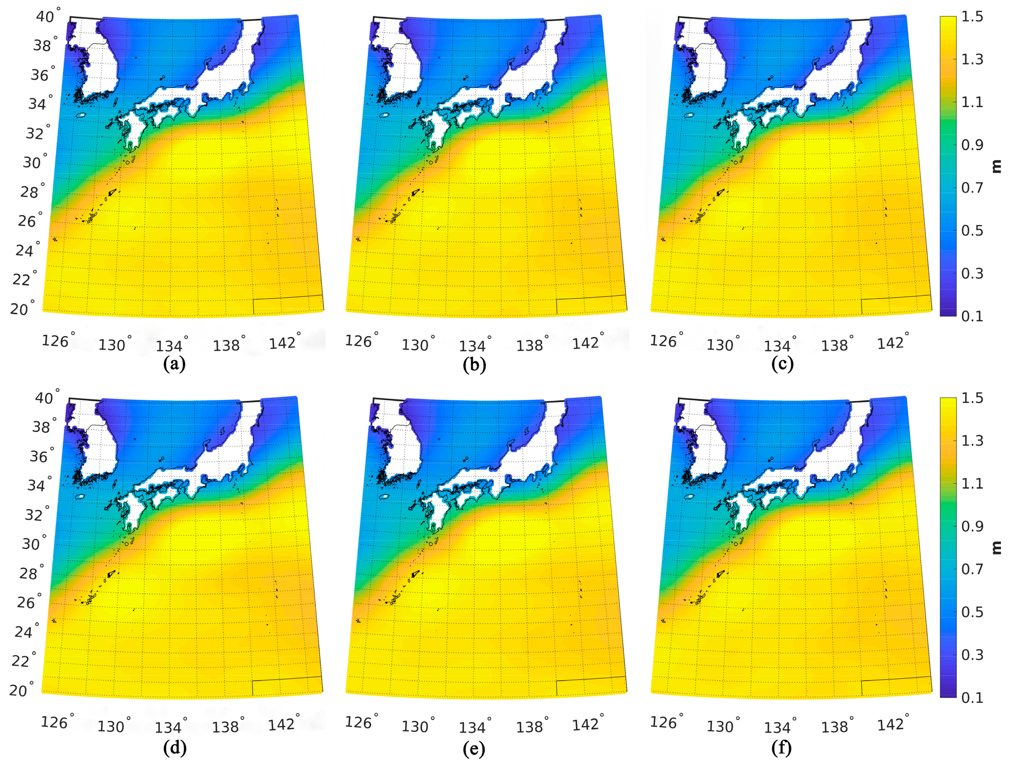
The MDTs solved by the OIM through the combination of the DTU18 MSS and GOCE-derived GGMs by means of the direct approach are shown in Figure 4, where Figure 4a–c are the MDTs based on the DIRR4, DIRR5, and DIRR6, denoted as DTU18DIRR4-MDT, DTU18DIRR5-MDT, and DTU18DIRR6-MDT, respectively; while Figure 4d–f are the time-wise solutions, which are denoted as DTU18TIMR4-MDT, DTU18TIMR5-MDT, and DTU18TIMR6-MDT, respectively. In order to verify the reliability of the MDT solutions, the reference MDT derived based on the average of the oceanographic and geodetic MDTs models; i.e., SODA, ORAS5, CNES-CLS13MDT, and Copernicus, were used for comparison. However, the evaluations of the error levels of the four MDTs, in addition to the reference MDT, were needed. Thus, these models were first referenced to 1993–2016; that is, the same as the buoy data, and the corresponding geostrophic ocean current was deduced and then compared with the in situ data, as shown in

Table 4. Statistics of the differences in the geostrophic velocities between the buoy data and the MDT models (units: mm/s).

MDT	COMPONENTS	MIN	MAX	RMS
SODA3	u	−758.2	497.0	113.0
	v	−619.8	541.7	94.5
ORAS5	u	−766.1	784.9	132.6
	v	−652.4	419.7	97.3
CNES-CLS13MDT	u	−724.2	539.8	113.4
	v	−647.6	478.0	93.4
Copernicus	u	−728.1	548.3	115.6
	v	−619.3	523.4	93.2
Reference MDT	u	−707.8	530.6	112.3
	v	−625.0	459.8	90.7

Note: the mean values of the misfit of the geostrophic velocity between the buoy data and the ocean models are removed.

. The results showed that the RMS of the difference between geostrophic current velocity derived from reference MDT and the buoy data was relatively smaller in comparison: 112 mm/s (91 mm/s) in the zonal (meridional) directions, respectively, which may be due to the smoothness of the noise. As a result, the reference MDT could be used for the comparative analysis in this study.

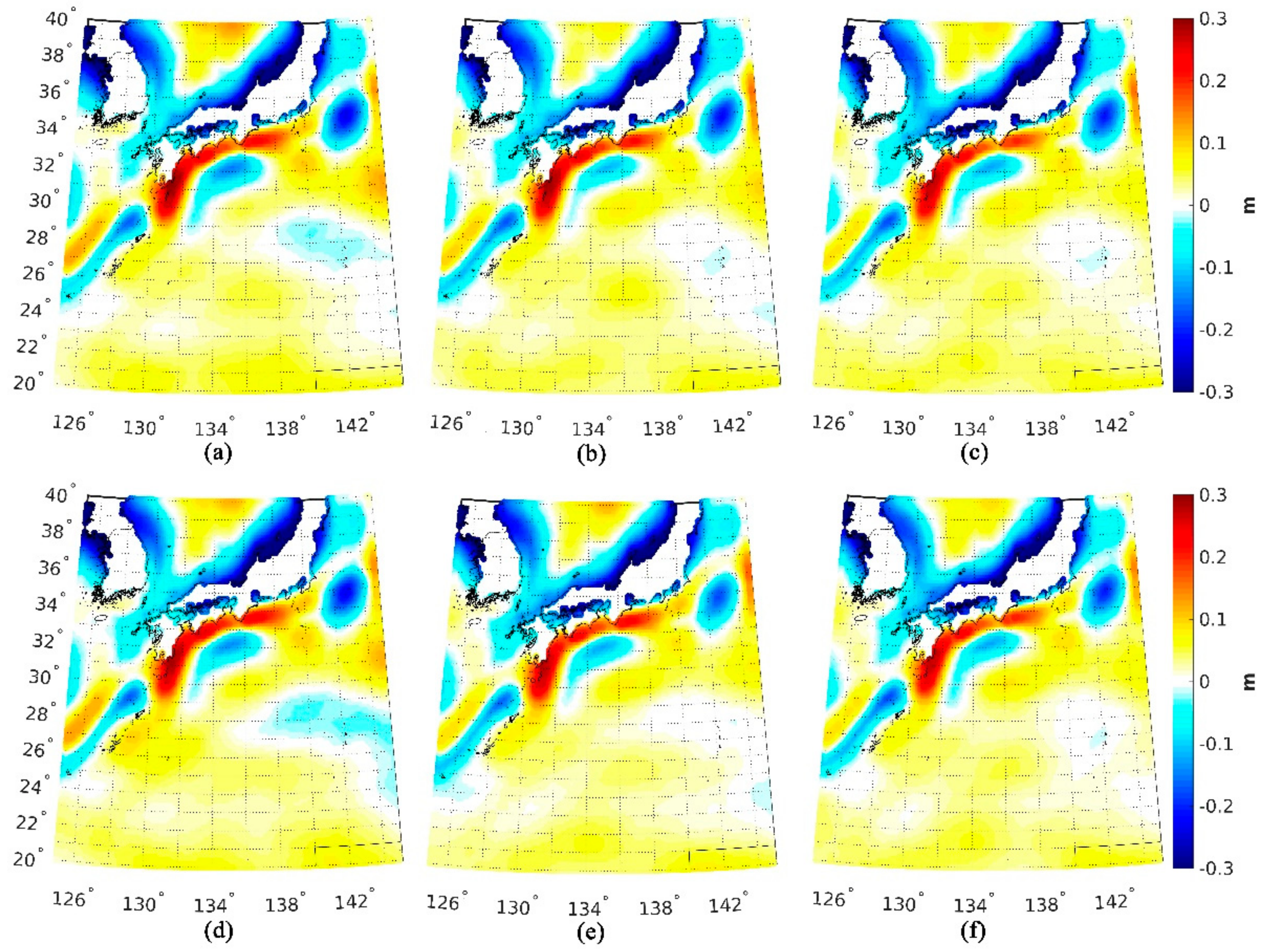
The differences between the reference MDT and the estimated MDTs are shown in Figure 5. It can be seen that the differences between the MDT solutions by OIM and the reference MDT were mainly concentrated in the current region in Figure 1, while there were fewer differences between the filtered MDT and reference MDT in most regions. This may be because the MDT models also were calculated through the filtering procedure, which screened out some of the detailed signals and is therefore not evident in Figure 5.

Table 5. Statistics of the differences between the reference MDTs and the estimated MDT (units: mm).

MDT Solutions	Min	Max	RMS
DTU18DIRR4-MDT	−434.6	292.6	82.4
DTU18DIRR5-MDT	−389.1	284.8	79.4
DTU18DIRR6-MDT	−383.3	270.2	77.0
DTU18TIMR4-MDT	−446.6	281.1	83.2
DTU18TIMR5-MDT	−402.5	272.7	78.0
DTU18TIMR6-MDT	−376.6	269.2	77.5

Note: the mean values of the misfit between the estimated MDTs and the reference MDT model are removed.

shows the statistical results of these comparisons (the mean differences are removed). The RMS of the difference between the DTU18DIRR6-MDT solution and reference MDT was 77.0 mm, which was 2.4 mm lower than that of the DTU18DIRR5-MDT solution and 5.4 mm lower than that of the DTU18DIRR4-MDT solution. In addition, the RMS of the difference between the DTU18TIMR6-MDT and reference MDT was 0.5 mm (5.7 mm) lower than that of DTU18TIMR5-MDT (DTU18TIMR4-MDT), suggesting that the development of the GGM could contribute to the MDT modeling. The recently satellite-only GGM was derived from all of the available GOCE gravity gradiometry data and recalibrated satellite orbit data. This illustrated that the accumulation of GOCE data and updated data preprocessing methods can be beneficial for MDT recovery.

3.2. MDT Solutions from Different DTU-Based MSS

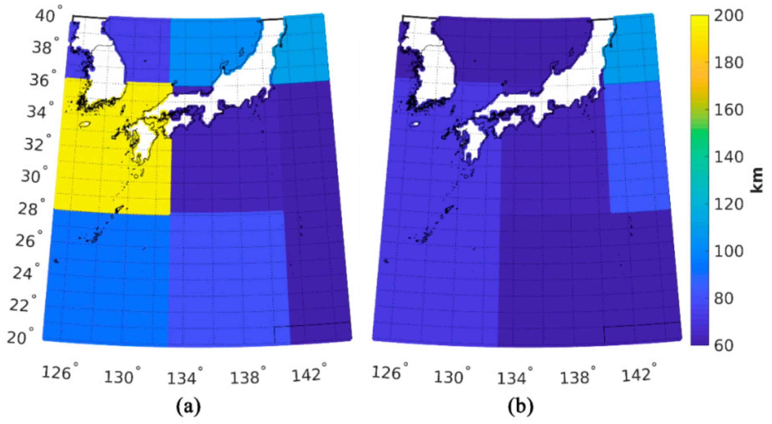
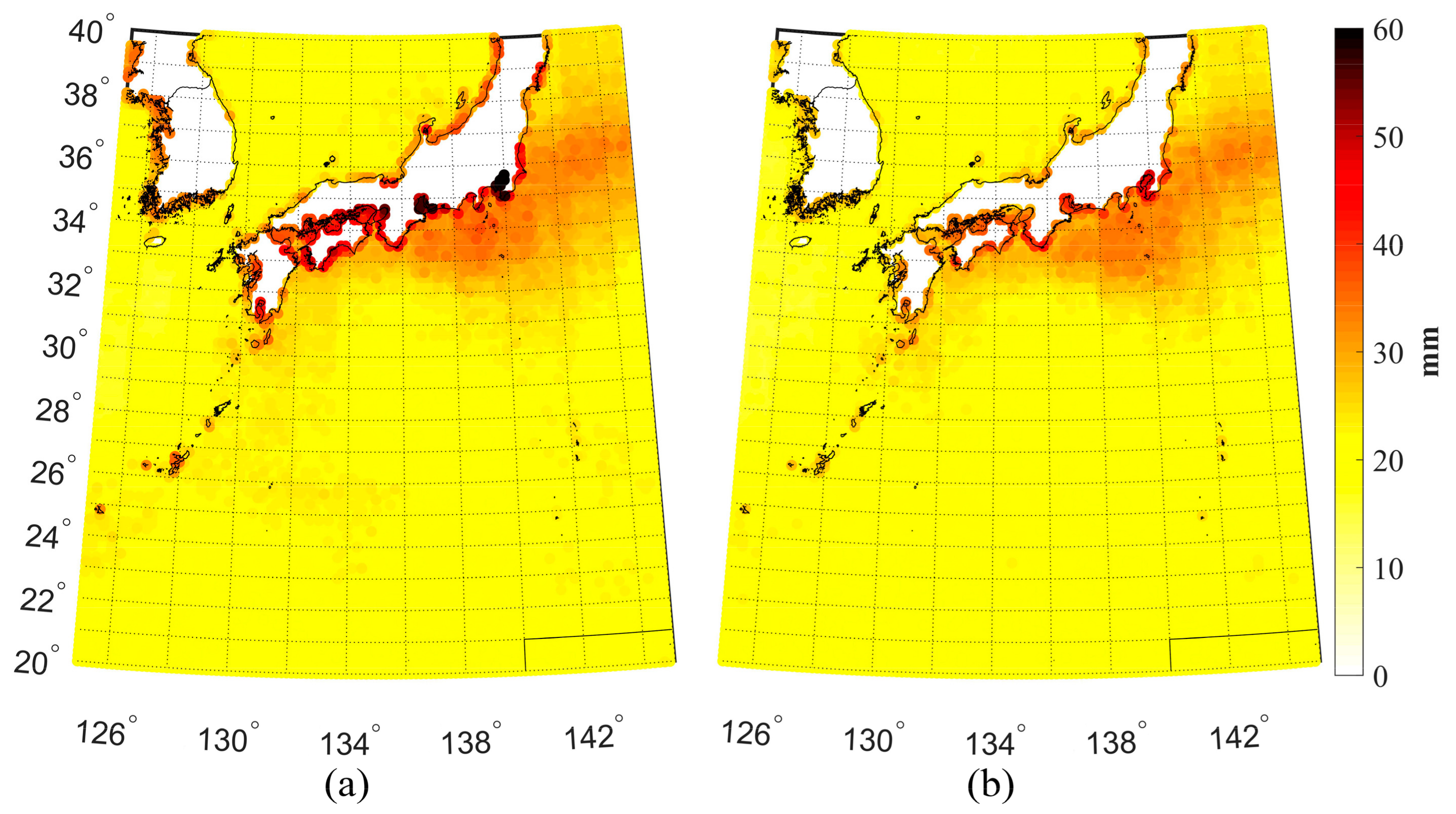
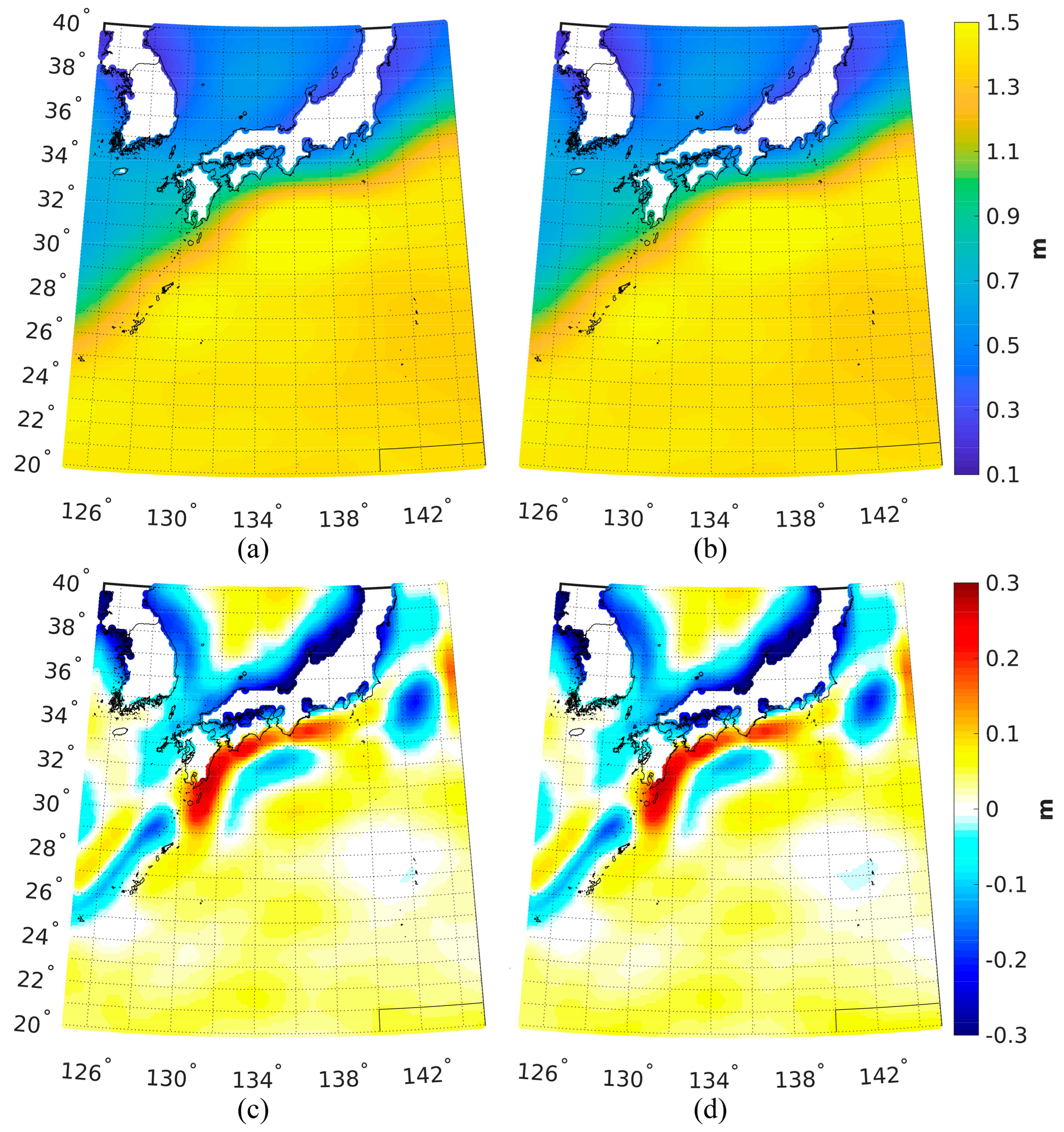
The selection of the MSS is of great importance to MDT modeling. In this case, the difference of the inputs of the OIM was the selection of MSS; therefore, the parameters such as the filtering radius of calculating the large-scale MDT and the prior MDT to estimate the variance and correlation function of the MDT were not considered. Although the accuracy of MSS in the open sea can reach the centimeter level [6], the accuracy of the MSS reduces rapidly near the coastal zone due to the defects of satellite altimetry. In this study, the DTU15 MSS and DTU18 MSS were used for MDT modeling, and the error distribution of the two MSSs is shown in Figure 6a,b, in which it can be seen that the error of DTU18 MSS was significantly smaller than that of DTU15 MSS, especially in the region around the coast.

Table 6. Statistics of the errors of the MSS models (units: mm).

MSS Models	Min	Max	Mean	RMS
DTU15 MSS	14.7	61.0	21.9	22.2
DTU18 MSS	13.5	48.0	20.7	21.1

gives the statistical information of the error of the MSS in the study area, and the accuracy of the DTU18 MSS improved by about 1 mm relative to the DTU15 MSS. The MDT solutions derived from the combination of the DIRR6 GGM and the DTU15 MSS, DTU18 MSS are shown in Figure 7a,b, and are denoted as DTU15DIRR6-MDT and DTU18DIRR6-MDT, respectively. It is shown that the two MDTs were similar to each other; thus, the reference MDT was used to perform the comparison, and the differences between the MDTs and the reference MDT are shown in Figure 7c,d. The statistical results of the differences are shown in

Table 7. Statistics of the differences between the estimated MDTs and the reference MDT (Units: mm).

MDT Solutions	Min	Max	RMS
DTU15DIRR6-MDT	−381.5	276.2	77.7
DTU18DIRR6-MDT	−383.3	270.2	77.0

Note: the mean values of the misfit between the estimated MDTs and the reference MDT model are removed.

(with the mean differences removed), from which we can see that the RMS of the difference between DTU18DIRR6-MDT and reference MDT was 0.7 mm smaller than that of DTU15DIRR6-MDT, which indicated that the improvement of MSS could not significantly improve the quality of the final MDT. The reason is that the improvement of the DTU18 MSS focused on the coastal area with respect to DTU15 MSS, but the improvement was limited in the other area.

3.3. Validation

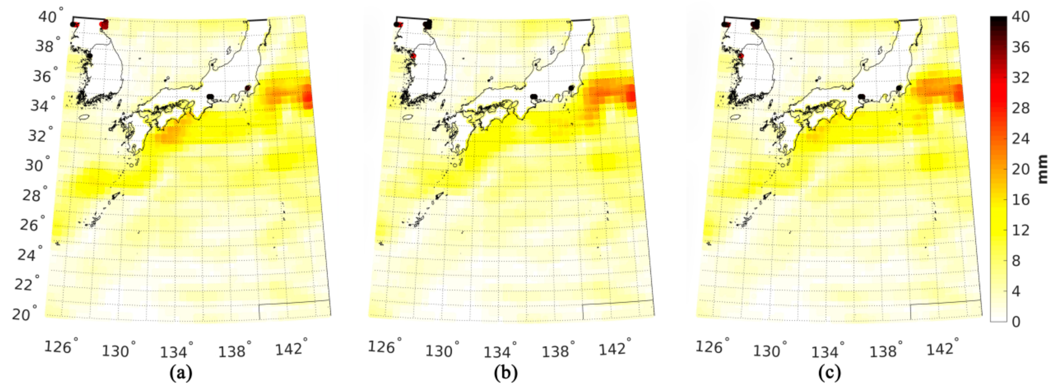
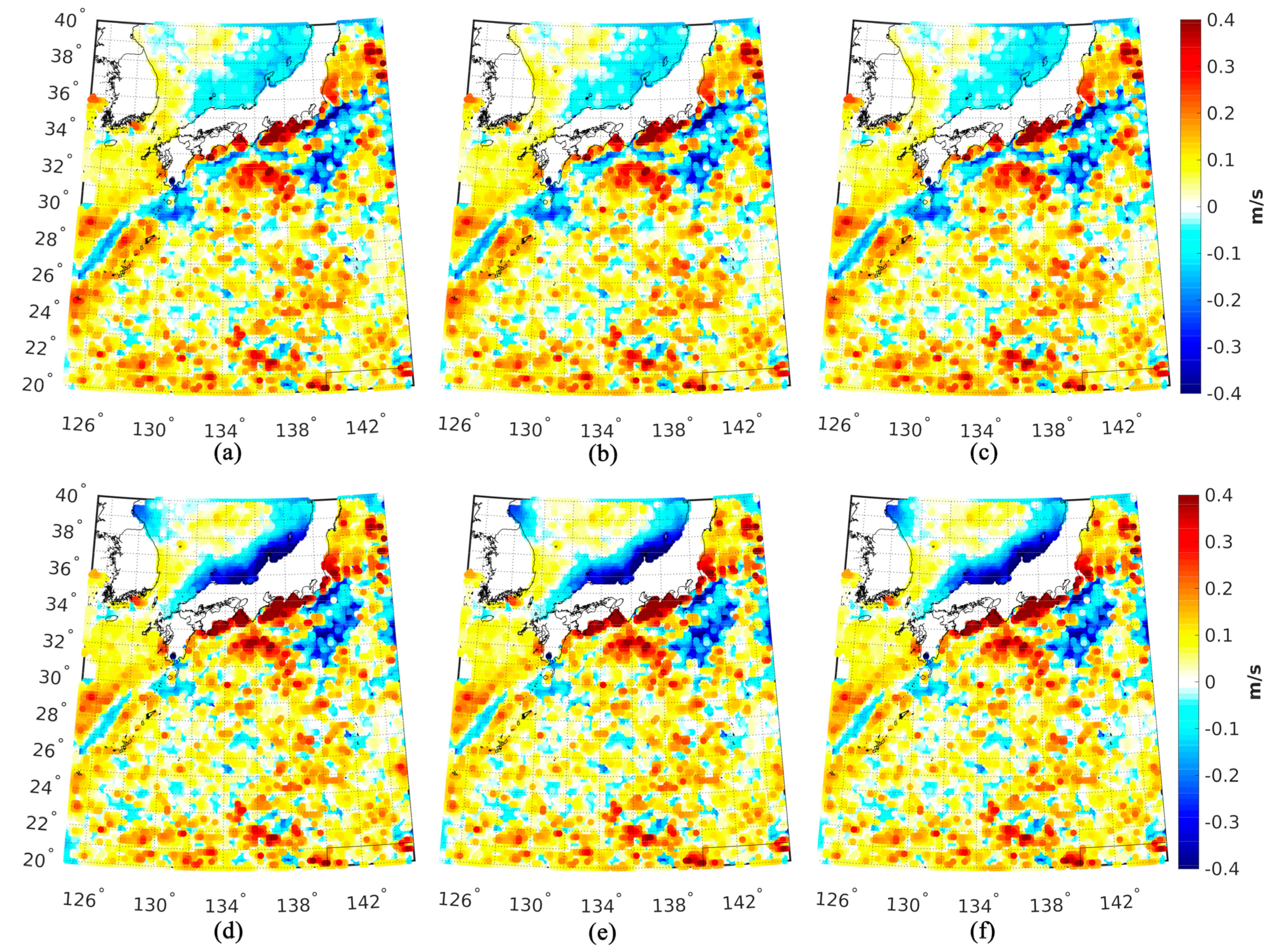
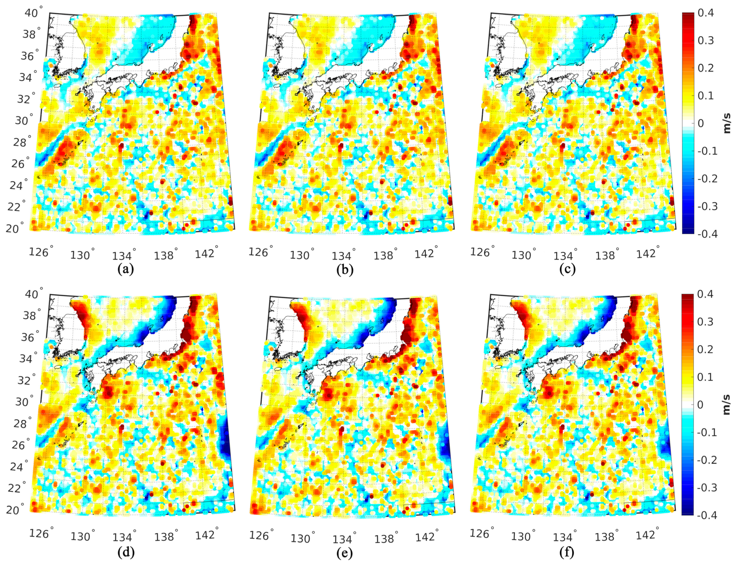
Compared to the Gaussian filtering method, one of the advantages is that the OIM can give the error distribution of the MDT based on the observations. Figure 8 shows the estimated error of the MDT calculated by the OIM, and the error was larger near the Kuroshio current. The RMS of the errors of DTU18DIRR4-MDT, DTU18DIRR5-MDT, and DTU18DIRR6-MDT was 6.1 mm, 6.0 mm, and 5.8 mm, respectively, which reflects the contribution of the improved GGM. Furthermore, in order to compare the OIM and Gaussian filter method, the MDTs based on DTU18 MSS and GOCE-derived GGMs were derived using a Gaussian filter method with a filter radius of 70 km [39], and the results were denoted as GF-R4-MDT, GF-R5-MDT, and GF-R6-MDT, respectively. The in situ geostrophic ocean current velocity profiles were used for validation, in which the reference time of the MDT solution; i.e., the DTU18DIRR4-MDT, DTU18DIRR5-MDT, DTU18DIRR6-MDT, GF-R4-MDT, GF-R5-MDT, and GF-R6-MDT, was unified to the same time period with the buoy data (1993–2016) using SLA provided by Aviso. Then, the associated geostrophic ocean current velocity was calculated using Equation (13). It was notable that the exportation of the geostrophic ocean current velocity from the MDT led to an error amplification [38], so a spatial filter was used to reduce the noise; the filter radius was selected as 60 km through experiments. In addition, the geostrophic ocean current velocity exported from the MDT was interpolated to the point of the buoy data, and the differences between them are shown in Figure 9 and Figure 10, where the differences in the zonal and meridional directions are shown, respectively. The geostrophic velocities derived from the OIM method had smaller misfits against the buoy data than those of the Gaussian filter method, especially in coastal areas. The statistical results of the difference are shown in

Table 8. Statistics of the differences in the geostrophic velocities between the buoy data and the information deduced from the MDT solutions (units: mm/s).

MDT Solutions	Geostrophic Velocity	Min	Max	RMS
DTU18DIRR4-MDT	u	−692.3	654.7	124.8
	v	−629.7	511.7	97.2
DTU18DIRR5-MDT	u	−698.5	646.8	123.8
	v	−629.3	510.4	95.5
DTU18DIRR6-MDT	u	−695.6	648.3	122.6
	v	−620.6	510.9	93.7
GF-R4-MDT	u	−707.7	766.6	133.4
	v	−675.9	651.6	119.3
GF-R5-MDT	u	−727.4	765.0	133.0
	v	−608.8	641.3	113.7
GF-R6-MDT	u	−722.6	763.9	132.9
	v	−622.9	637.2	110.8

Note: the mean values of the misfit of the geostrophic velocity between the buoy data and the MDT models are removed.

, in which it can be seen that the RMS of the differences between the DTU18DIRR6-MDT-derived zonal (meridional) components and the in situ data were 122.6 mm/s (93.7 mm/s), which were 1.2 mm/s (1.8 mm/s) lower than that of the DTU18DIRR5-MDT, and 2.2 mm/s (3.5 mm/s) lower than that of the DTU18DIRR4-MDT. In addition, when making the comparison between the OIM solution and the Gaussian filtered solution, the RMS of the difference between the zonal (meridional) geostrophic ocean current velocity derived from the Gaussian filtered solution against the in situ data were about 10 mm/s (17 mm/s) larger than those of the OIM solution, which indicated that the OIM was better than the Gaussian filtering method. The comparison between Table 8 and Table 4 shows that the RMS of the difference between the geostrophic ocean current velocity of the MDT models and the in situ data was about 10 mm/s lower than that of the estimated MDT, which indicated that the accuracy of the MDT models was similar to the estimated MDT.

4. Conclusions

We studied the optimal interpolation method for regional MDT recovery based on GOCE-derived GGMs and mean sea surface. In particular, the performances of different GGMs in MDT recovery were studied, and the contributions introduced from the recently released GOCE-derived GGMs were quantified and assessed. Moreover, the choice of MSS model was investigated, and the effects on MDT modeling introduced from different MSS models were quantified. In addition, we compared the traditionally used Gaussian filtering method with the optimal interpolation method in regional MDT modeling. The numerical results over the Kuroshio showed that:

(1)

The use of the recently released GOCE-derived GGM improved the accuracy of the computed MDT. The RMS of the difference between the MDT derived from sixth-generation GOCE-derived GGM modeled by the direct approach and independent ocean data was reduced by a magnitude of 5.4 mm (2.4 mm), compared to the result derived from the fourth-generation (fifth-generation) model.

(2)

The choice of recently published MSS models may have had limited effects on MDT recovery. The RMS of the difference between the MDT modeled from DTU18MSS and ocean data was only 0.7 mm lower than that computed from DTU15MSS.

(3)

For further comparison, the buoy data was introduced, and the geostrophic velocities derived from DTU18MSS and different GOCE-derived GGMs were compared with the buoy data. The results revealed that the RMS of the differences between the zonal (meridional) velocities derived from the sixth-generation GGM and buoy data were 1.2 mm/s (1.8 mm/s) less than that derived from the fifth-generation model, and 2.2 mm/s (3.5 mm/s) less than the fourth-generation GGM, respectively. This also suggested that the improvements in the GGM could contribute to the accuracy improvement of the MDT modeling.

(4)

Moreover, the numerical experiments showed that the optimal interpolation method outperformed the Gaussian filtering approach, in which the geostrophic velocity derived from the optimal interpolation method had a smaller misfit against the buoy data by a magnitude of 10 mm/s (17 mm/s) when the zonal (meridian) component was validated. This was mainly due to the optimal interpolation method using the error information of the input data, which may have obtained more reasonable weights of observations than the Gaussian filtering method.

References

- Wu, Y.; Abulaitijiang, A.; Featherstone, W.E.; McCubbine, J.C.; Andersen, O.B. Coastal gravity field refinement by combining airborne and ground-based data. J. Geod. 2019, 93, 2569–2584. [Google Scholar] [CrossRef]
- Hwang, C.; Hsu, H.J.; Featherstone, W.E.; Cheng, C.C.; Yang, M.; Huang, W.; Wang, C.Y.; Huang, J.F.; Chen, K.H.; Huang, C.H.; et al. New gravimetric-only and hybrid geoid models of Taiwan for height modernisation, cross-island datum connection and airborne LiDAR mapping. J. Geod. 2020, 94, 1–22. [Google Scholar] [CrossRef]
- He, Y.C.; Gao, Y.Q.; Wang, H.J.; Ola, J.M.; Yu, L. Transport of nuclear leakage from Fukushima nuclear power plant in the north pacific. Acta Oceanol. Sin. 2012, 34, 12–20. [Google Scholar] [CrossRef]
- Wu, Y.; Luo, Z. The approach of regional geoid refinement based on combining multi-satellite altimetry observations and heterogeneous gravity data sets. Chin. J. Geophys. 2016, 59, 1596–1607. [Google Scholar] [CrossRef]
- Rio, M.H.; Hernandez, F. A mean dynamic topography computed over the world ocean from altimetry, in situ measurements, and a geoid model. J. Geophys. Res. Oceans 2004, 109. [Google Scholar] [CrossRef] [Green Version]
- Chambers, D.P. Evaluation of new GRACE time-variable gravity data over the ocean. Geophys. Res. Lett. 2006, 33. [Google Scholar] [CrossRef]
- Wu, Y.; Zhou, H.; Zhong, B.; Luo, Z. Regional gravity field recovery using the GOCE gravity gradient tensor and heterogeneous gravimetry and altimetry data. J. Geophys. Res. Solid Earth 2017, 122, 6928–6952. [Google Scholar] [CrossRef]
- Kornfeld, R.P.; Arnold, B.W.; Gross, M.A.; Dahya, N.T.; Klipstein, W.M.; Gath, P.F.; Bettadpur, S. GRACE-FO: The gravity recovery and climate experiment follow-on mission. J. Spacecr Rockets 2019, 56, 931–951. [Google Scholar] [CrossRef]
- Eppelbaum, L.; Katz, Y.; Klokochnik, J.; Kosteletsky, J.; Zheludev, V.; Ben-Avraham, Z. Tectonic Insights into the Arabian-African Region inferred from a Comprehensive Examination of Satellite Gravity Big Data. Glob. Planet. Chang. 2018, 171, 65–87. [Google Scholar] [CrossRef]
- Bruinsma, S.L.; Förste, C.; Abrikosov, O.; Lemoine, J.M.; Marty, J.C.; Mulet, S.; Rio, M.H.; Bonvalot, S. ESA’s satellite-only gravity field model via the direct approach based on all GOCE data. Geophys Res. Lett. 2014, 41, 7508–7514. [Google Scholar] [CrossRef] [Green Version]
- Andersen, O.; Knudsen, P.; Stenseng, L. A New DTU18 MSS Mean Sea Surface—Improvement from SAR Altimetry. In Proceedings of the 25 Years of Progress in Radar Altimetry Symposium, Ponta Delgada, Azores, Portugal, 24–29 September 2018. [Google Scholar]
- Knudsen, P.; Bingham, R.; Andersen, O.; Rio, M.H. A global mean dynamic topography and ocean circulation estimation using a preliminary GOCE gravity model. J. Geod. 2011, 85, 861–879. [Google Scholar] [CrossRef]
- Wang, W.; Wen, H.; Liu, H.; Chen, B.; Jia, X. A method for determining high-precision geostrophic currents in the eastern seas of China. Sci. Surv. Mapp. 2019, 44, 37–43. [Google Scholar] [CrossRef]
- Zhang, Z.; Lu, Y.; Hsu, H. Detecting surface geostrophic currents using wavelet filter from satellite geodesy. Sci. China Ser. D Earth Sci. 2007, 50, 918–926. [Google Scholar] [CrossRef]
- Vianna, M.L.; Menezes, V.V.; Chambers, D.P. A high resolution satellite-only GRACE-based mean dynamic topography of the South Atlantic Ocean. Geophys. Res. Lett. 2007, 34, L24604. [Google Scholar] [CrossRef] [Green Version]
- Rio, M.H.; Guinehut, S.; Larnicol, G. New CNES-CLS09 global mean dynamic topography computed from the combination of GRACE data, altimetry, and in situ measurements. J. Geophys. Res. Oceans 2011, 116. [Google Scholar] [CrossRef]
- Förste, C.; Abrykosov, O.; Bruinsma, S.; Dahle, C.; König, R.; Lemoine, J.M. ESA’s Release 6 GOCE Gravity Field Model by Means of the Direct Approach Based on Improved Filtering of the Reprocessed Gradients of the Entire Mission (GO_CONS_GCF_2_DIR_R6); Data Publication; GFZ Data Services: Potsdam, Germany, 2019. [Google Scholar] [CrossRef]
- Joh, Y.; Di Lorenzo, E. Interactions between Kuroshio Extension and Central Tropical Pacific lead to preferred decadal-timescale oscillations in Pacific climate. Sci. Rep. 2019, 9, 13558. [Google Scholar] [CrossRef] [Green Version]
- Brockmann, J.M.; Schubert, T.; Schuh, W.D. An Improved Model of the Earth’s Static Gravity Field Solely Derived from Reprocessed GOCE Data. Surv. Geophys. 2021, 42, 277–316. [Google Scholar] [CrossRef]
- Gruber, T. GOCE Release 6 Products and Performance. In Proceedings of the 27th IUGG General Assembly, Presentation, Montreal, QC, Canada, 8–18 July 2019. [Google Scholar]
- Bingham, R.J.; Haines, K. Mean dynamic topography: Intercomparisons and errors. Philos. Trans. R. Soc. A 2006, 364, 903–916. [Google Scholar] [CrossRef]
- Carton, J.A.; Chepurin, G.A.; Chen, L. SODA3: A new ocean climate reanalysis. J. Clim. 2018, 31, 6967–6983. [Google Scholar] [CrossRef]
- Zuo, H.; Balmaseda, M.A.; Tietsche, S.; Mogensen, K.; Mayer, M. The ECMWF operational ensemble reanalysis–analysis system for ocean and sea ice: A description of the system and assessment. Ocean. Sci. 2019, 15. [Google Scholar] [CrossRef] [Green Version]
- The Climate Data Store. Available online: https://cds.climate.copernicus.eu/cdsapp#!/dataset/satellite-sea-level-global?tab=doc (accessed on 20 May 2020).
- Rio, M.H.; Mulet, S.; Picot, N. Beyond GOCE for the ocean circulation estimate: Synergetic use of altimetry, gravimetry, and in situ data provides new insight into geostrophic and Ekman currents. Geophys. Res. Lett. 2014, 41, 8918–8925. [Google Scholar] [CrossRef]
- Lumpkin, R.; Johnson, G.C. Global ocean surface velocities from drifters: Mean, variance, El Niño–Southern Oscillation response, and seasonal cycle. J. Geophys. Res. Oceans 2013, 118, 2992–3006. [Google Scholar] [CrossRef]
- Laurindo, L.C.; Mariano, A.J.; Lumpkin, R. An improved near-surface velocity climatology for the global ocean from drifter observations. Deep Sea Res. 1 Oceanogr. Res. Pap. 2017, 124, 73–92. [Google Scholar] [CrossRef]
- Bretherton, F.P.; Davis, R.E.; Fandry, C.B. A technique for objective analysis and design of oceanographic experiments applied to MODE-73. Deep Sea Res. Oceanogr. Abstr. 1976, 23, 559–582. [Google Scholar] [CrossRef]
- Arhan, M.; De Verdiére, A.C. Dynamics of eddy motions in the eastern North Atlantic. J. Phys. Oceanogr. 1985, 15, 153–170. [Google Scholar] [CrossRef] [Green Version]
- Balmino, G. Efficient propagation of error covariance matrices of gravitational models: Application to GRACE and GOCE. J. Geod. 2009, 83, 989–995. [Google Scholar] [CrossRef]
- Gilardoni, M.; Reguzzoni, M.; Sampietro, D. GECO: A global gravity model by locally combining GOCE data and EGM2008. Stud. Geophys. Geodaet. 2016, 60, 228–247. [Google Scholar] [CrossRef]
- Pavlis, N.K. An Earth Gravitational model to degree 2160: EGM08. In Proceedings of the 2008 General Assembly of the European Geosciences Union, Vienna, Austria, 13–18 April 2008. [Google Scholar]
- Liang, W.; Xu, X.; Li, J.; Zhu, G. The determination of an ultra high gravity field model SGG-UGM-1 by combining EGM2008 gravity anomaly and GOCE observation data. Acta Geodaet. Cartogr. Sin. 2018, 47, 425–434. [Google Scholar] [CrossRef]
- Pail, R.; Fecher, T.; Barnes, D.; Factor, J.F.; Holmes, S.A.; Gruber, T.; Zingerle, P. Short note: The experimental geopotential model XGM2016. J. Geod. 2018, 92, 443–451. [Google Scholar] [CrossRef]
- Bingham, R.J.; Haines, K.; Lea, D.J. How well can we measure the ocean’s mean dynamic topography from space? J. Geophys. Res. Oceans 2014, 119, 3336–3356. [Google Scholar] [CrossRef] [Green Version]
- Asheghi, R.; Hosseini, S.A.; Saneie, M.; Shahri, A.A. Updating the neural network sediment load models using different sensitivity analysis methods: A regional application. J. Hydroinform. 2020, 22, 562–577. [Google Scholar] [CrossRef] [Green Version]
- Rio, M.H.; Pascual, A.; Poulain, P.M.; Menna, M.; Barceló, B.; Tintoré, J. Computation of a new mean dynamic topography for the Mediterranean Sea from model outputs, altimeter measurements and oceanographic in situ data. Ocean. Sci. 2014, 10, 731–744. [Google Scholar] [CrossRef] [Green Version]
- Bai, X.; Yan, H.; Zhu, Y. GOCE steady-state sea surface dynamic terrain and geostrophic circulation based on regional filtering. Chin. J. Geophys. 2015, 58, 1535–1546. [Google Scholar] [CrossRef]
- Andersen, O.; Knudsen, P.; Stenseng, L. The DTU13 MSS (mean sea surface) and MDT (mean dynamic topography) from 20 years of satellite altimetry. In IGFS2014; Springer: Cham, Switzerland, 2015; pp. 111–121. [Google Scholar] [CrossRef]
Figure 1.
The study area is identified by a red dotted rectangle, and the solid red line represents the Kuroshio current. The Kuroshio passes through the Luzon Strait, and the majority flows northward along the east coast of Taiwan into the East China Sea. Then it flows out of the East China Sea from the Tukara Strait, and finally flows eastward offshore near 35° N, becoming the Kuroshio extension.
Figure 2.
The error degree variance in geoid height calculated with different GOCE-derived GGMs.
Figure 3.
The correlation radii in (a) zonal and (b) meridional of the study area.
Figure 4.
The estimated MDT based on (a) DIRR4, (b) DIRR5, (c) DIRR6, (d) TIMR4, (e) TIMR5, and (f) TIMR6.
Figure 5.
The differences between (a) DTU18DIRR4-MDT, (b) DTU18DIRR5-MDT, (c) DTU18DIRR6-MDT, (d) DTU18TIMR4-MDT, (e) DTU18 TIMR5MDT, (f) DTU18TIM R6-MDT and the reference MDT.
Figure 6.
The error distribution of (a) DTU15 MSS; (b) DTU18 MSS.
Figure 7.
The MDTs of the (a) DTU15DIRR6-MDT and (b) DTU18DIRR6-MDT, and the corresponding differences between them and the reference MDT (c,d).
Figure 8.
The estimated errors the MDT solutions (a) DTU18DIRR4-MDT; (b) DTU18DIRR5-MDT; (c) DTU18DIRR6-MDT.
Figure 9.
The differences in zonal geostrophic velocities between buoy data and information deduced from the MDT solutions: (a) DTU18DIRR4-MDT; (b) DTU18DIRR5-MDT; (c) DTU18DIRR6-MDT; (d) GF-R4-MDT; (e) GF-R5-MDT; (f) GF-R6-MDT.
Figure 10.
The differences in meridional geostrophic velocities between buoy data and information deduced from the MDT solutions: (a) DTU18DIRR4-MDT; (b) DTU18DIRR5-MDT; (c) DTU18DIRR6-MDT; (d) GF-R4-MDT; (e) GF-R5-MDT; (f) GF-R6-MDT.