
Fractional Order Processing of Satellite Images


1
IDMEC, Instituto Superior Técnico, Universidade de Lisboa, Av. Rovisco Pais, 1049-001 Lisboa, Portugal
2
ICT, Escola de Ciências e Tecnologia, Universidade de Évora, Rua Romão Ramalho 59, 7000-671 Évora, Portugal
*
Author to whom correspondence should be addressed.
†
These authors contributed equally to this work.
Appl. Sci. 2021, 11(11), 5288; https://0-doi-org.brum.beds.ac.uk/10.3390/app11115288
Submission received: 11 May 2021
/
Revised: 31 May 2021
/
Accepted: 1 June 2021
/
Published: 7 June 2021
(This article belongs to the Special Issue Novel Advances of Image and Signal Processing)
Abstract
:Nowadays, satellite images are used in many applications, and their automatic processing is vital. Conventional integer grey-scale edge detection algorithms are often used for this. This study shows that the use of color-based, fractional order edge detection may enhance the results obtained using conventional techniques in satellite images. It also shows that it is possible to find a fixed set of parameters, allowing automatic detection while maintaining high performance.
Keywords:
satellite images; fractional derivative; automatic detection; color-based detection; grey-scale detection; fractional processing; aerospace; very-high-resolution satelliteMSC:
26A33; 68U10; 94A081. Introduction
1.1. Objective and Contribution
Image processing has always been an essential tool in remote sensing. Processed images taken by satellites allow extracting relevant information in fields like land monitoring, routine mapping and surveillance [1].
Edge detection represents an important role in remote sensing. The conventional edge detectors are based on integer derivatives. With the introduction of fractional calculus, some new non-integer edge detectors were created and the existent integer ones adapted [2].
The aforementioned detectors were developed for grey-scale images. Since colored images are often available, a simple solution is to convert them to grey-scale, but this may compromise the performance of edge detection and discards potentially relevant information. Thus, color-based edge detection detectors were created [3,4].
Algorithms for edge detection methods often involve first or second order derivatives, which can be generalised using a fractional order derivative instead [5]. The goal of this paper is to apply fractional edge detection to satellite images, verifying how appropriate these algorithms are for the job. To assess this, results obtained with fractional order algorithms applied to color images are compared with those of conventional integer order algorithms, for both color and grey-scale images. Another important point to assess performance is whether or not it is possible to use fixed parameters to treat all the images. Experiences with medical images, for which optimal parameters have very disparate values, and are hardly predictable in advance, suggest that this may be an issue [6]. So the contribution of this paper is to show that fractional derivatives achieve good results in image treatment of satellite images with parameters automatically set.
1.2. Previous Work on Fractional Image Processing
Fractional derivatives, defined below in Section 2.2, are studied in depth in [7,8,9]. Their application to image processing began in 2002 with the CRONE method [10]. Since then, a few already extant image treatment methods have been adapted to include fractional derivatives (instead of usual, integer order derivatives), such as the fractional Roberts operator [11], the fractional Sobel method [12,13], the fractional Canny method [6], or the fractional Laplacian of Gaussian method [14]. These methods will be addressed below in Section 2 and details can be found in [5].
1.3. Satellite Image Data
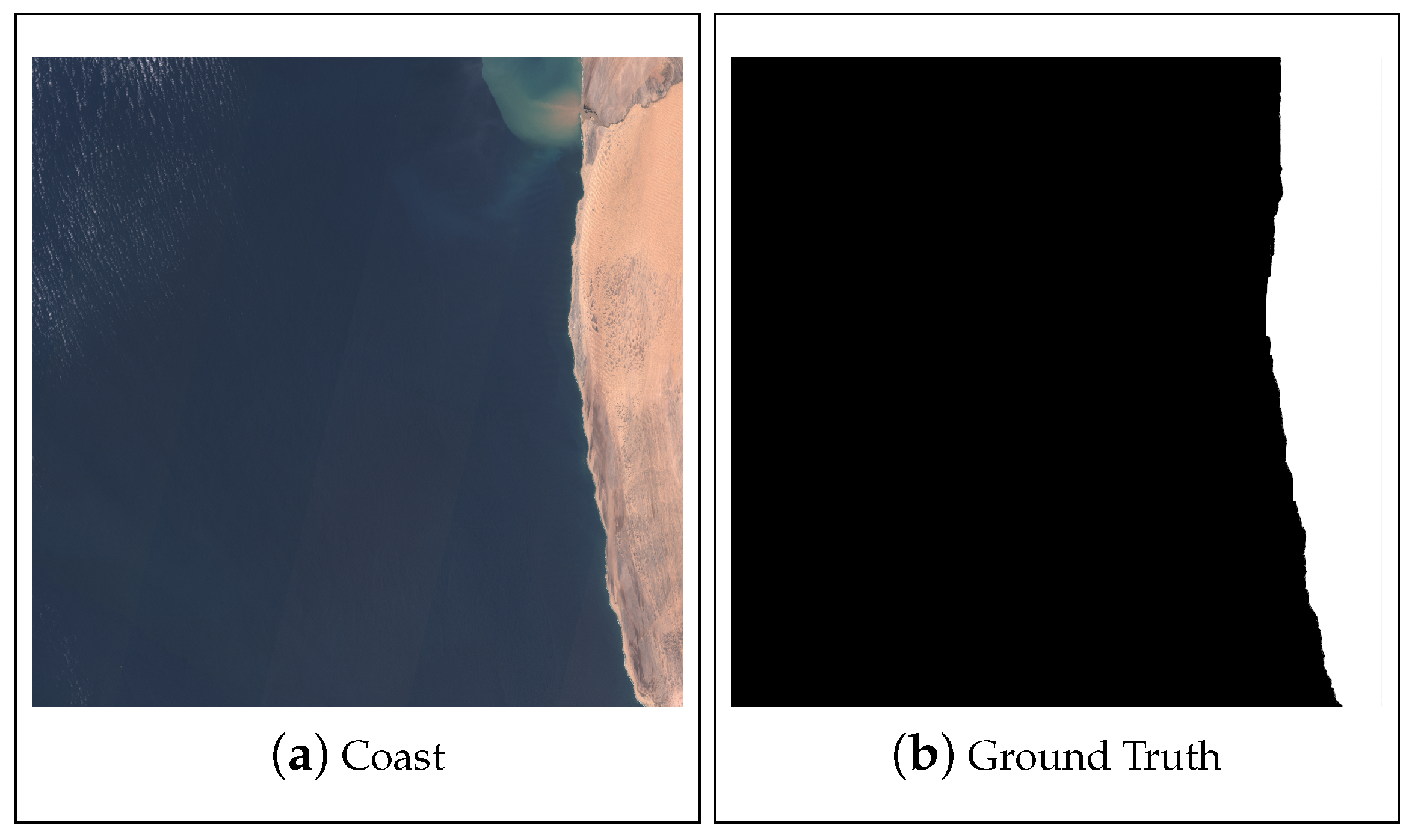
In this paper, forty-three random images with low nebulosity from ESA’s Sentinel-2 satellite [19] were used. The images retrieved from the website were analysed and a ground truth was manually taken using GIMP. The satellite images database, as well as the detailed extended results of this study, are available in an online repository [20].
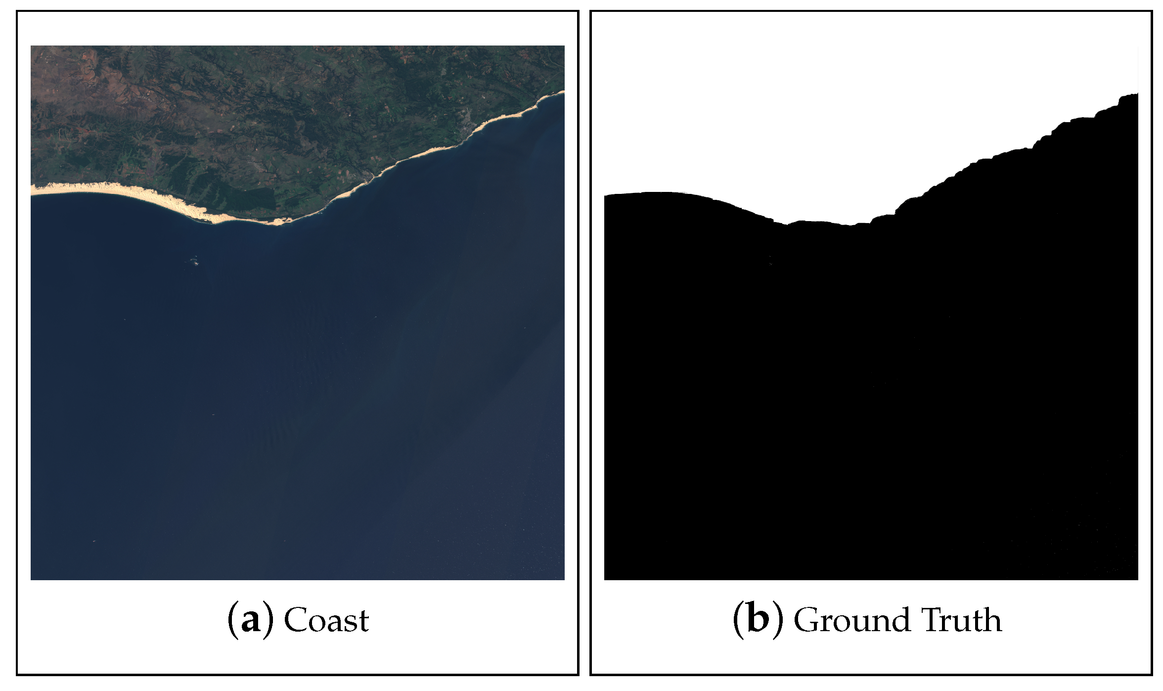
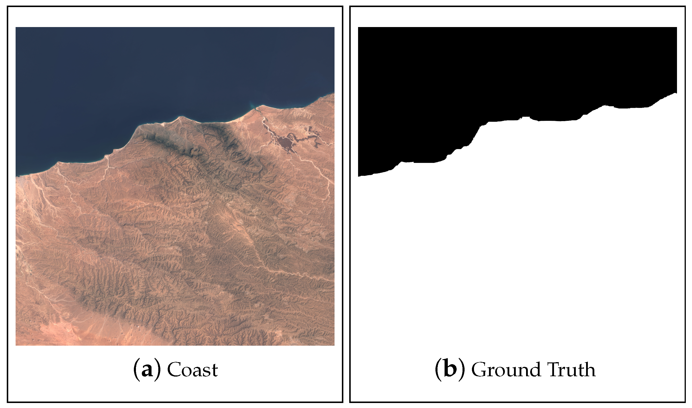
Due to space reasons, from the forty three figures, four were chosen to illustrate performance in this paper. The selected images are numbers 12, 18, 27 and 38. These pictures were selected since they present different levels of global performance due to their heterogeneity and are shown in Figure 1, Figure 2, Figure 3 and Figure 4 together with their corresponding ground truth.
1.4. Paper Organisation
2. Definitions and Formulations
This section presents and compares the image treatment algorithms.
2.1. Main Algorithm Description
A main script was developed where the different edge detectors were introduced:
- The image to be processed is read.
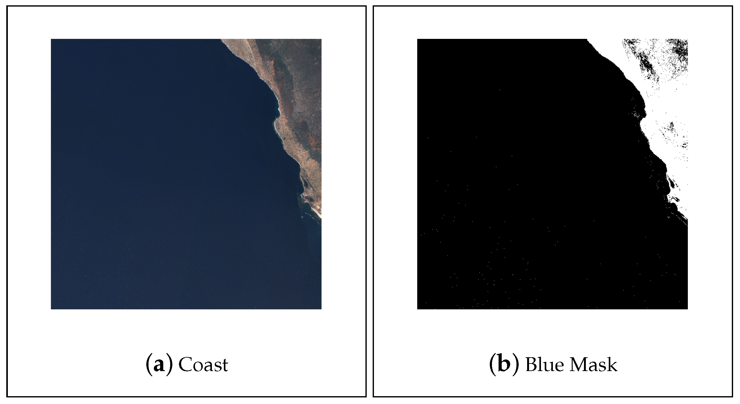
- A pre-processing step is performed where the figure is scanned for blue color pixels. A mask is formed attributing value zero to all blue pixels found. This mask is later used in post-processing (Figure 5), both for the case of grey-scale detection operators, and the case of color detection operators.
- One of the edge detection operators described in the next subsection is applied to the image. If the operator is to be applied to a grey-scale image, it must be converted first; Figure 6 shows the case when the image is converted to grey-scale for comparison purposes.
- After contour detection it is necessary to close the contours, so that in the end segmentation of land and water is evident. For that, several closing morphological operations are performed.
- Firstly, using lines in , , and directions a closing operation is carried out in order to close pixel gaps between nearby edges that the detector did not encounter.
- Next, in order to fill the parts of land that were not yet detected by the operator and the closing operations, a MATLAB built-in function is used (imfill).
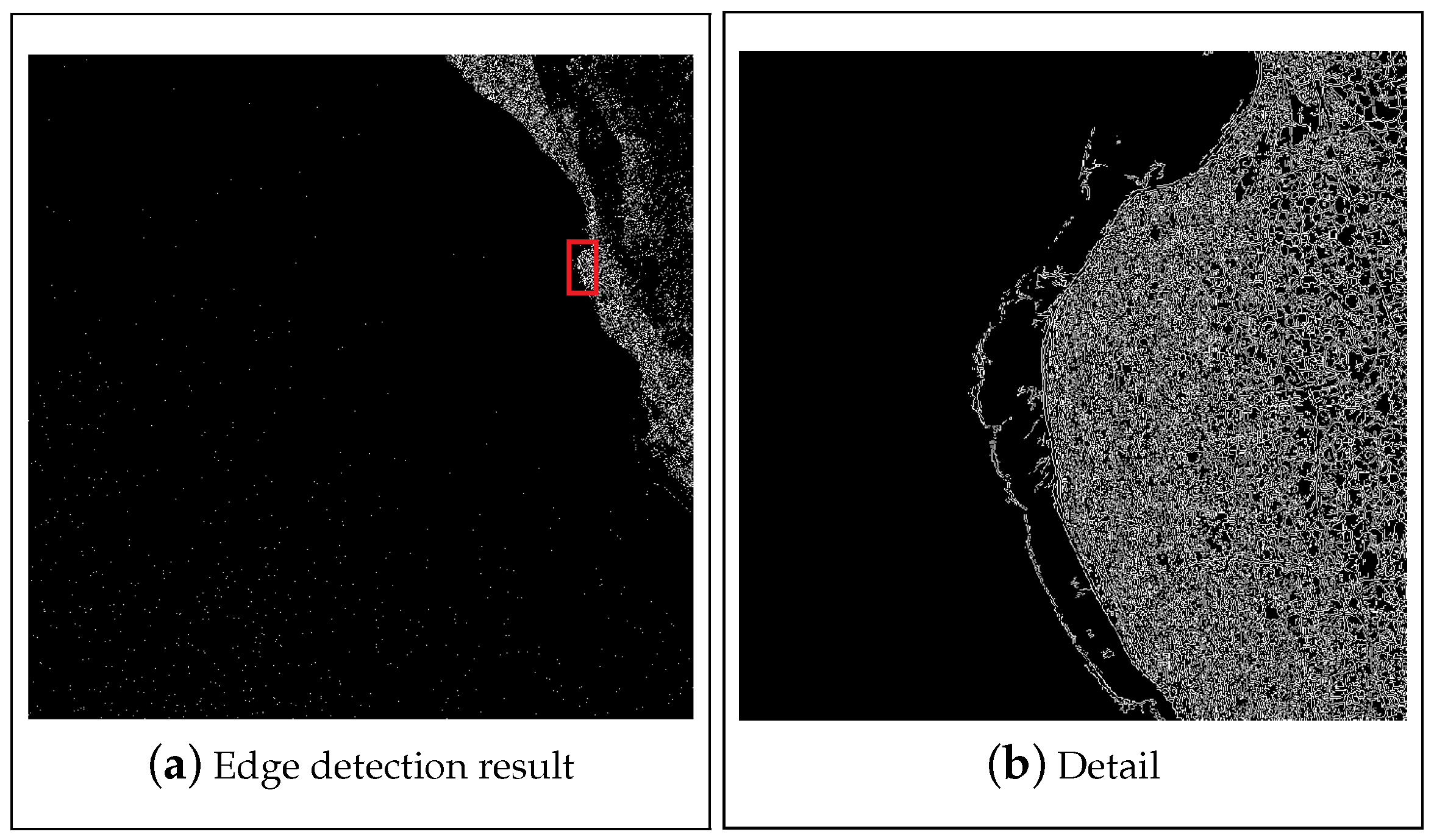
- The blue mask obtained in the pre-processing is then applied to the result of the previous operations. As one can see in Figure 6, after the edge detection there is still a lot of noise in the water. The blue mask serves as a filter that eliminates this noise and guarantees better performance in segmentation.
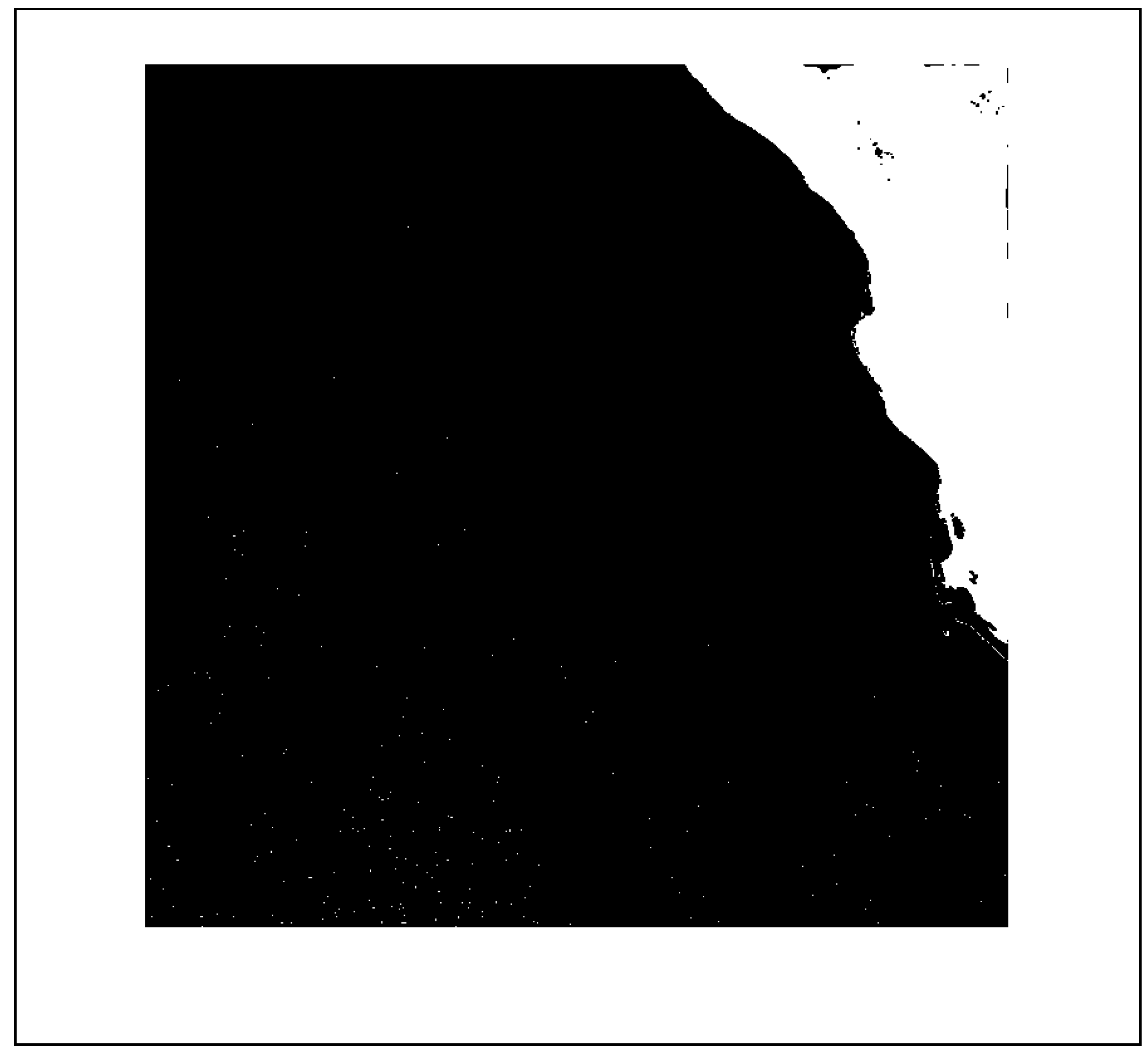
- One last closing operation is performed. This is due to the fact that sometimes the color filter identifies small areas of land as blue. Using this closing operation, these small areas are set to white and are correctly identified. This step finalizes the processing part of the algorithm. An example of a processed image is shown in Figure 7.
- After post-processing, performance analysis is done. For this, the ground truth jpg image is read and converted to a logical array. Then, by comparison between the resultant processed image and the ground truth, four metrics of performance are computed. The results of this analysis are stored in an array and are ready for analysis.
2.2. Edge Detection Operators
All the edge detection operators used in the algorithm above make use of the Grünwald-Letnikoff definition of fractional derivative:
where combinations of a things, b at a time, are given by [21]
The operators employed were the following. They are further detailed in [5].
- Canny Edge Detector. In this popular edge detection algorithm [22], the image is first convolved with a Gaussian Filter, and then a derivative operator is applied to the smoothed image to compute gradients. This is done determining the first partial derivatives of the smoothed image in both the x and y directions for each color channel, defining the following Jacobian [3]:The direction in the image along which the largest variation in the chromatic image function occurs is represented by the eigenvector of corresponding to the largest eigenvalue.
- Sobel Edge Detector. The integer Sobel operator performs a derivative operation on an image and so it highlights regions where there are sudden increases of pixel intensity which correspond to edges, and consists of the two masks [23]The fractional Sobel operator given in [13] has the maskA novel color-based fractional Sobel was implemented by applying the same algorithm of the Canny deterctor, with the mask in (7).
- The fractional Roberts detector presented in [11] and based on the truncated coefficients of the GL definition applies derivatives of arbitrary order :This mask is applied after the convolution of an image with the conventional integer Sobel. A color-based version of this detector was developed using the same approach as the Sobel algorithm. Since the fractional operator requires two convolutions, the color-based computations were applied only to the first one with the integer mask. After this, the result is convolved with (9).
- Laplacian of Gaussian (LoG) Detector. Three possible Laplacian operators areTo tackle the sensitivity of second order derivatives to noise, in the LoG the image is Gaussian smoothed before applying the Laplacian filter reducing high frequency noise. The smoothing filter can also be convolved first with the Laplacian kernel and only then is the result convolved with the input image. In the fractional case [14],For color images [25], a pixel is considered as part of an edge if zero-crossings are found in any of the color channels. Using this definition, an algorithm that detects edges in color images was developed. The algorithm convolves each channel of the input color image with the LoG mask in (11). Then, a search for zero-crossings in the results for each channel is performed. If any zero-crossings are found, the corresponding pixels are flagged as part of an edge.
- In order to detect edges on images, the formulated detector can be used in two dimensions with maskand its transpose. Color is handled as for the Canny operator.
- Fractional Derivative Operator. Fractional mask (9) from the Roberts operator was used in this paper by itself as a fractional edge detector. For color images, the Jacobian is reduced to a vectorand the magnitude of the gradients is given by
3. Results
In this section, the overall relevant results of the iterations with different parameters will be presented, and illustrated with the four images shown in Section 1.3. Again, the results for all the forty-three images in the database are available in repository [20].
3.1. Performance Assessment
In order to check performance, quantification has to be made. For that, the ground truth is compared to the output of the algorithm by scanning all pixels within the image. Four instances may occur: True Positives, False Positives, True Negatives and False Negatives (Table 1).
Using the number of occurrences of each instance the following metrics were computed:
During the study it was concluded that the Jaccard coefficient (J) is a good overall performance metric since the results with the highest J corresponded to the ones with maximum mean performance regarding the four metrics. Thus, the Jaccard coefficient is used as overall performance indicator.
3.2. Performance Analysis of Fractional vs. Integer Edge Detection
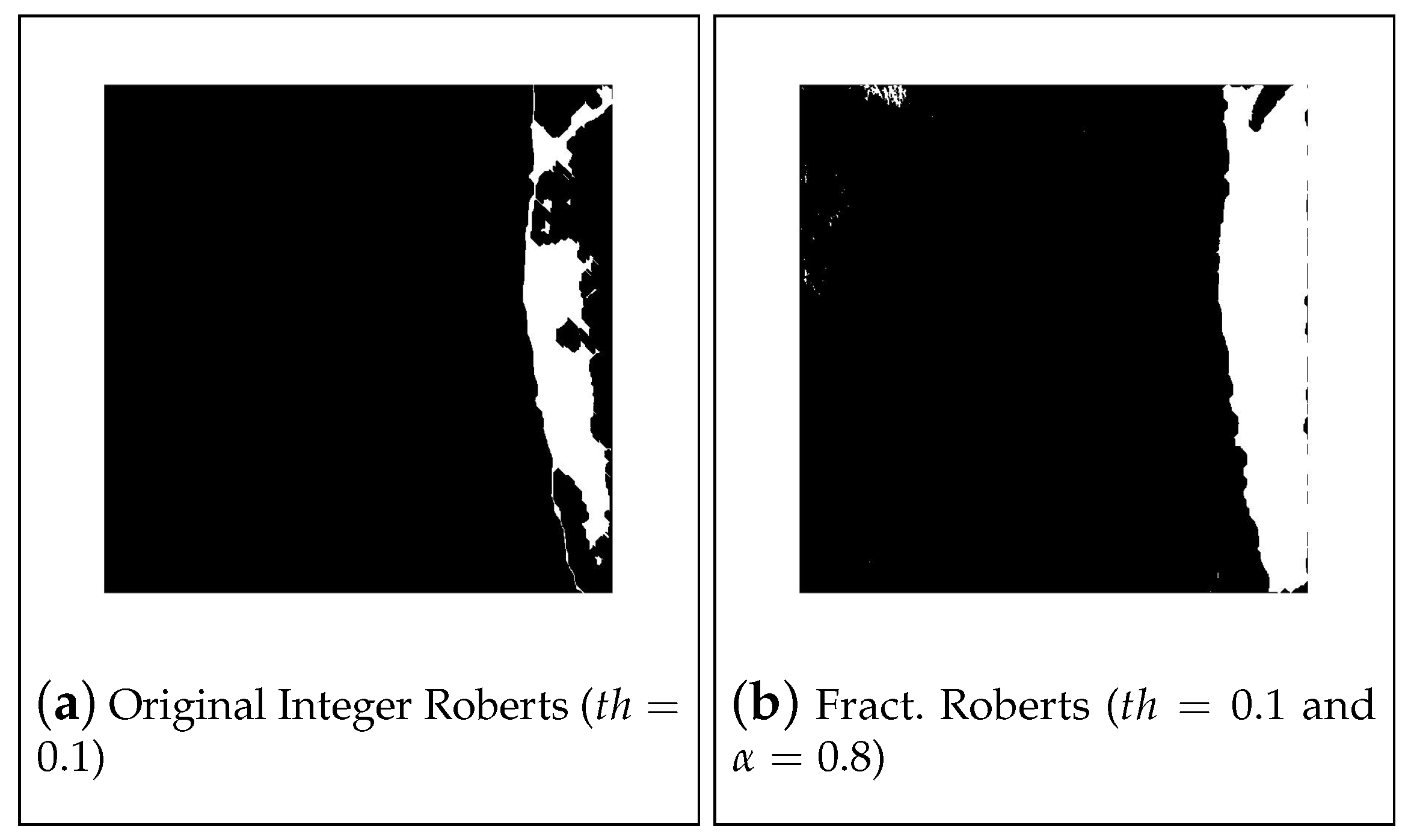
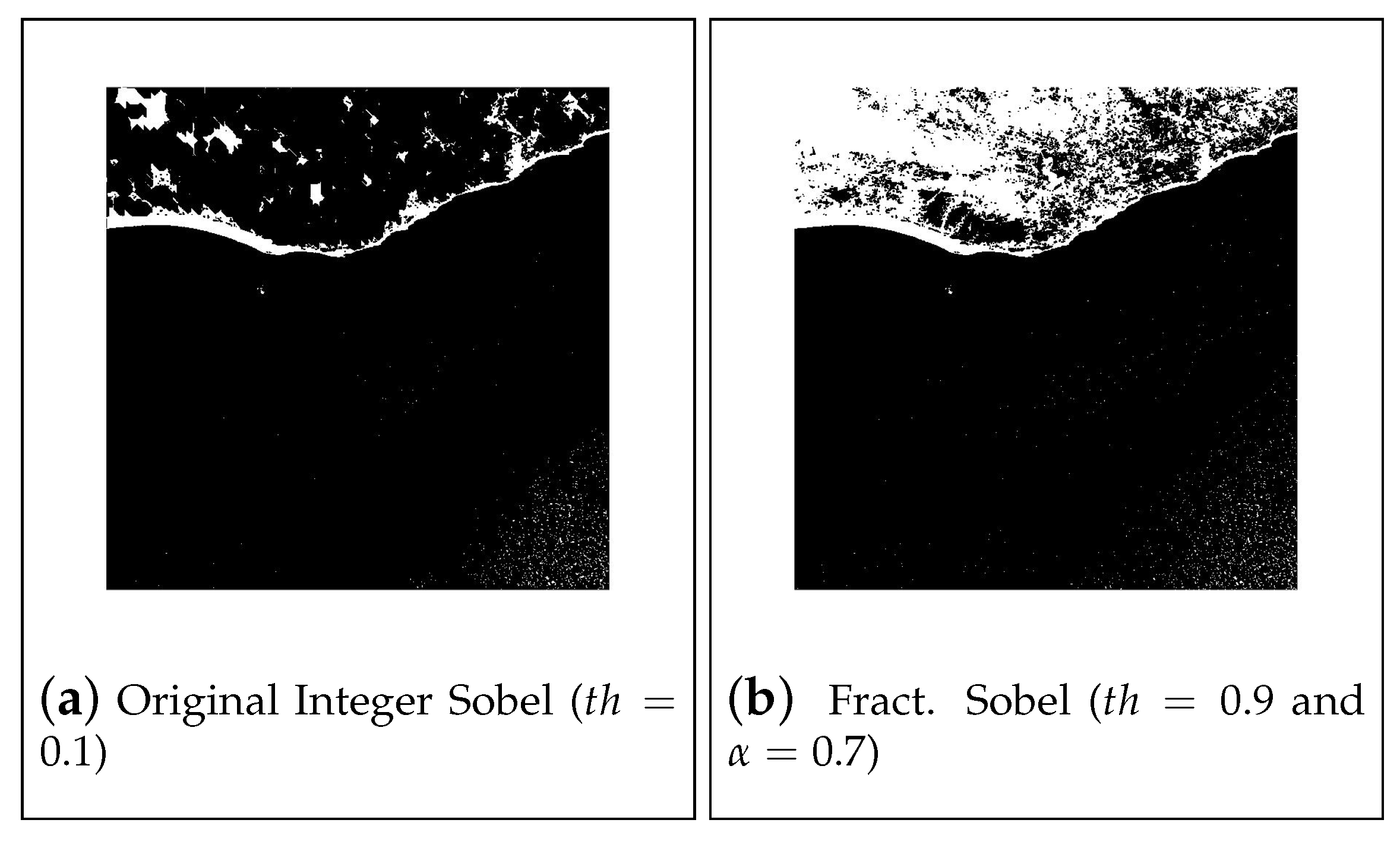
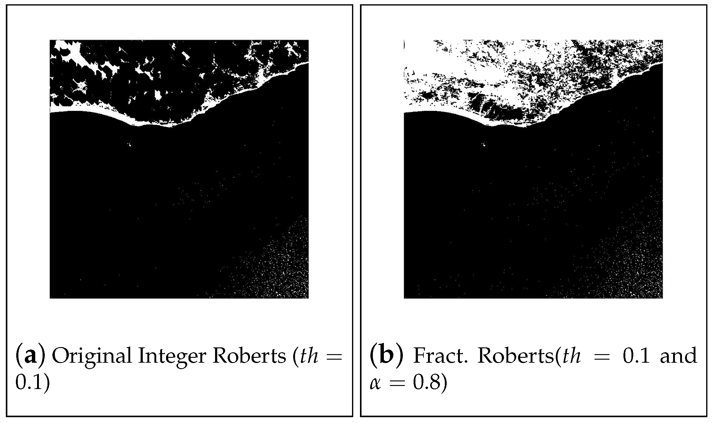
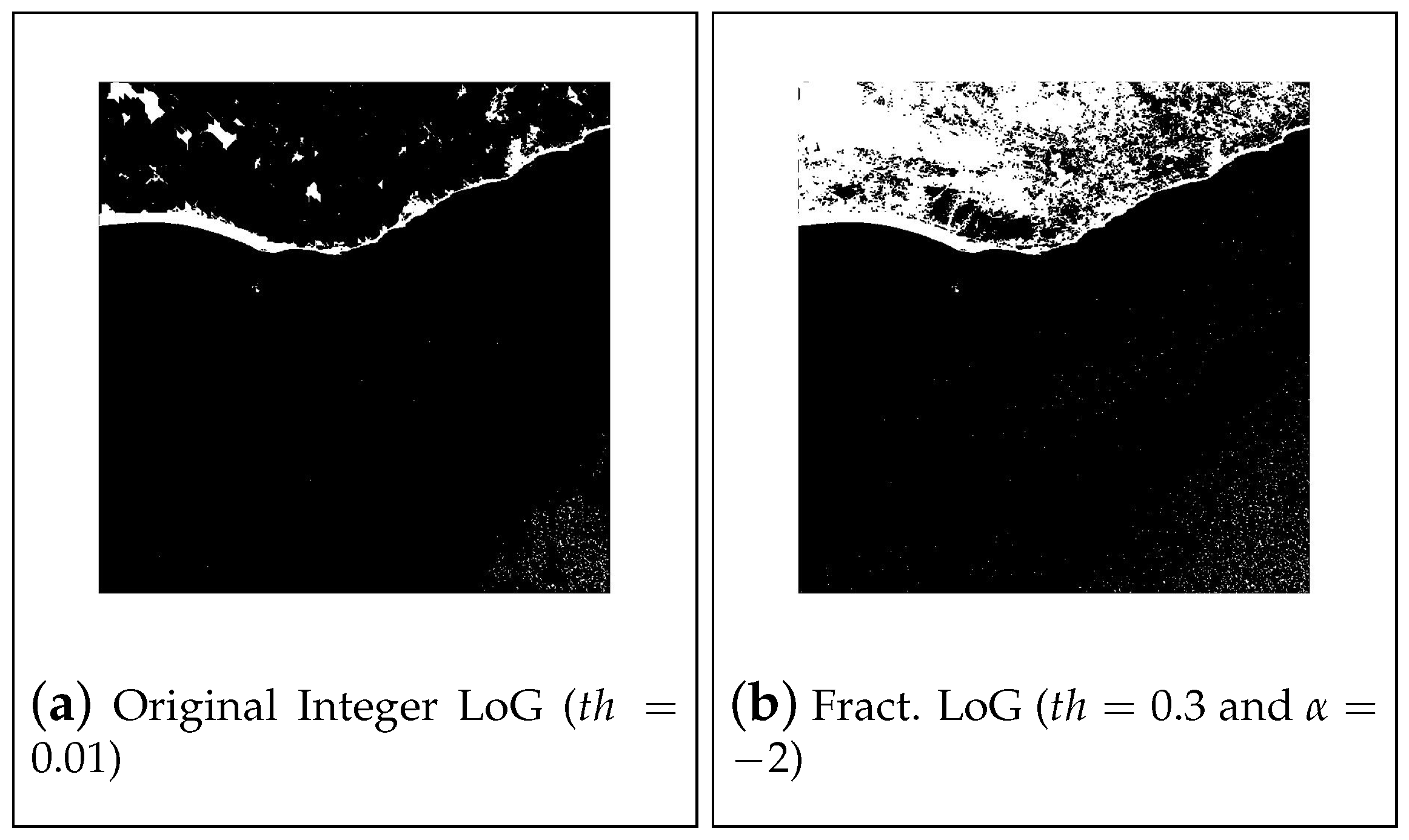
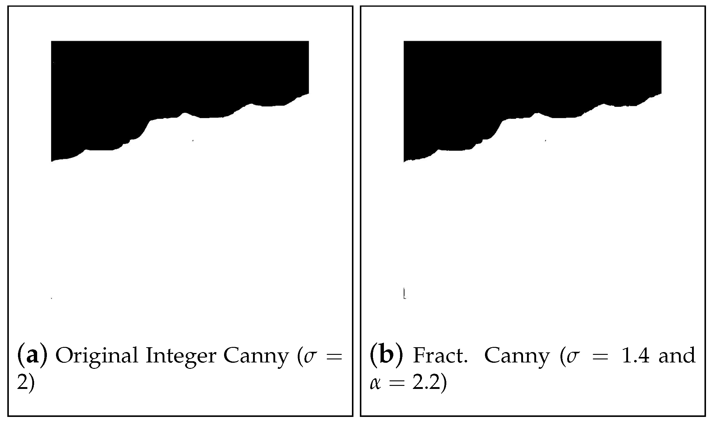
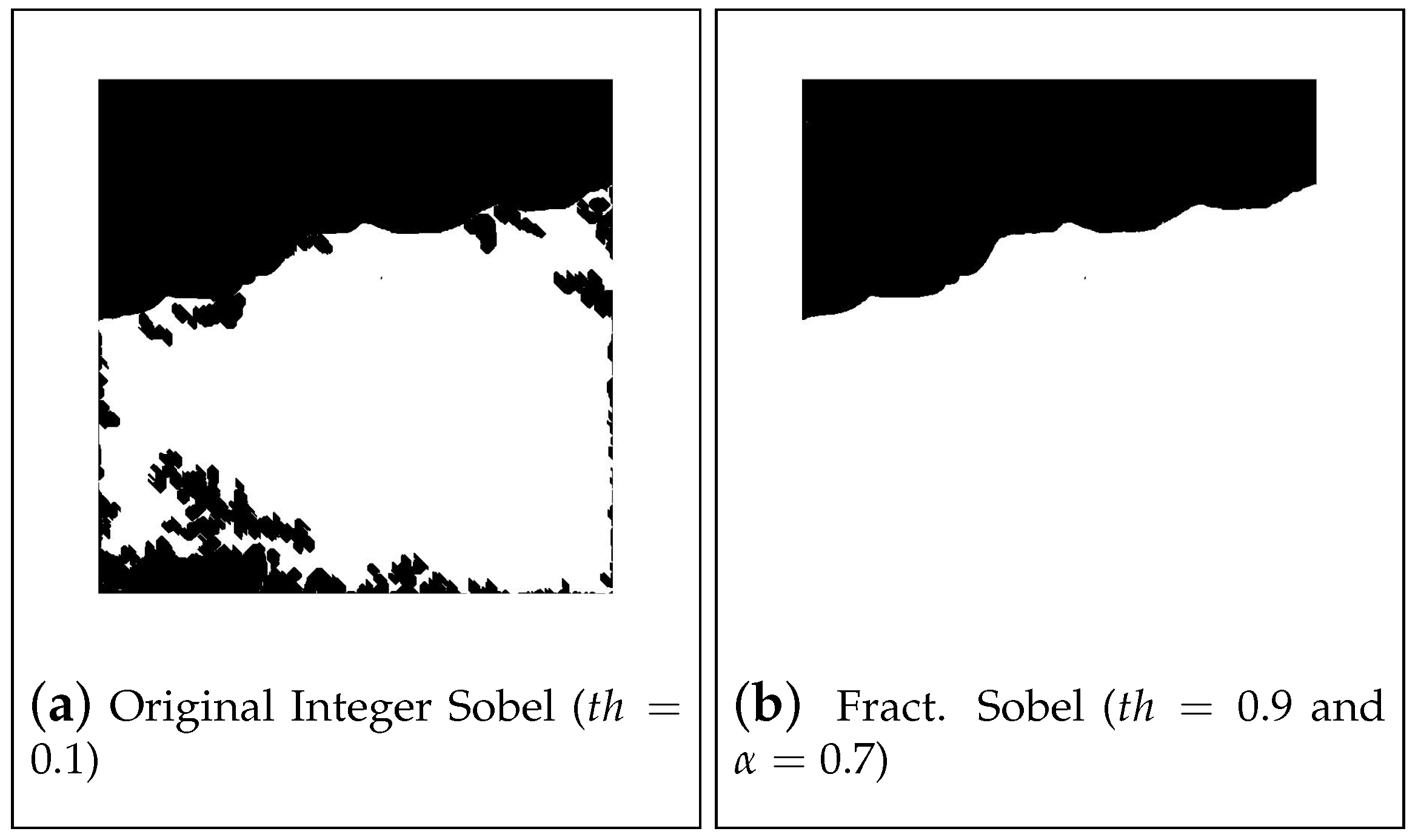
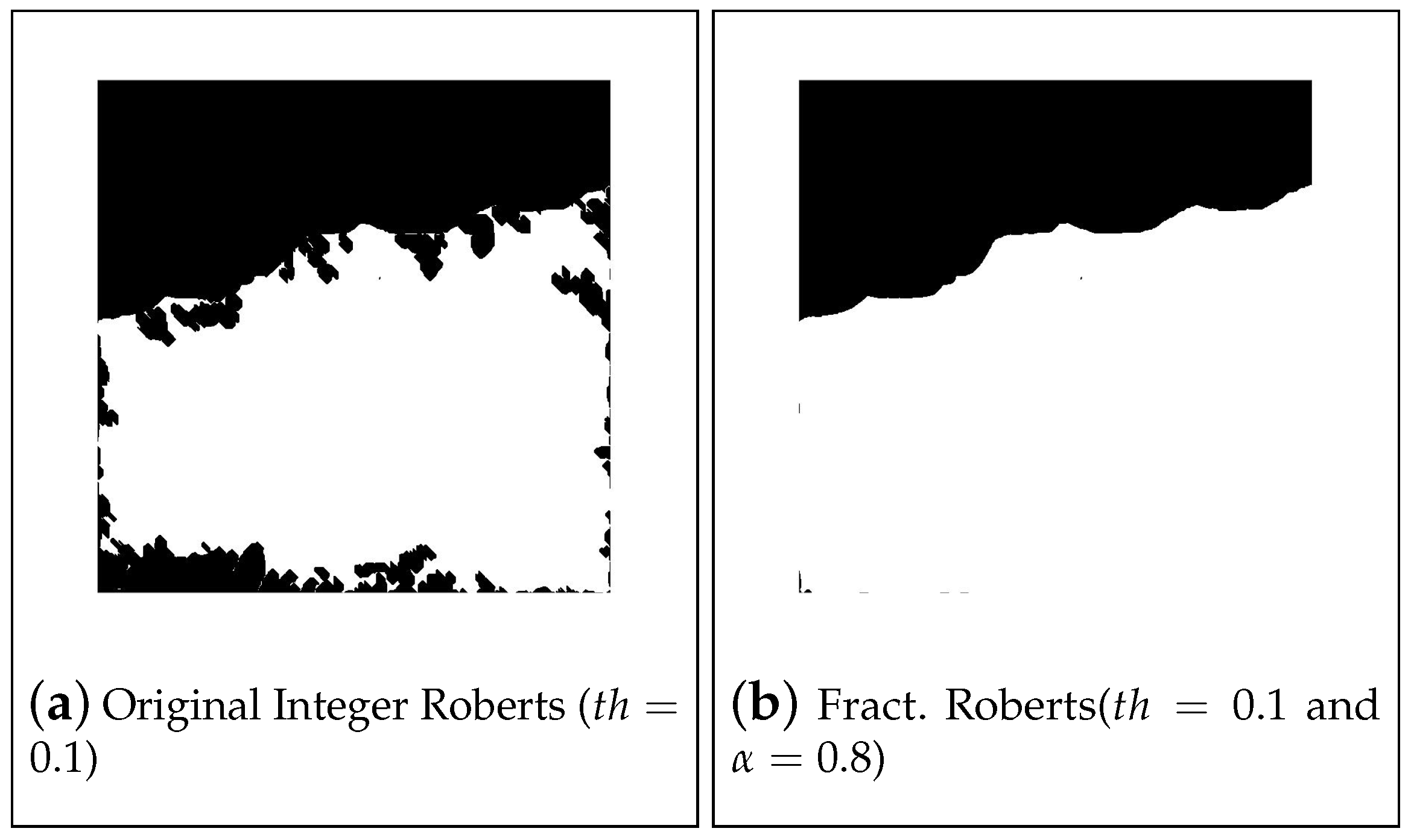
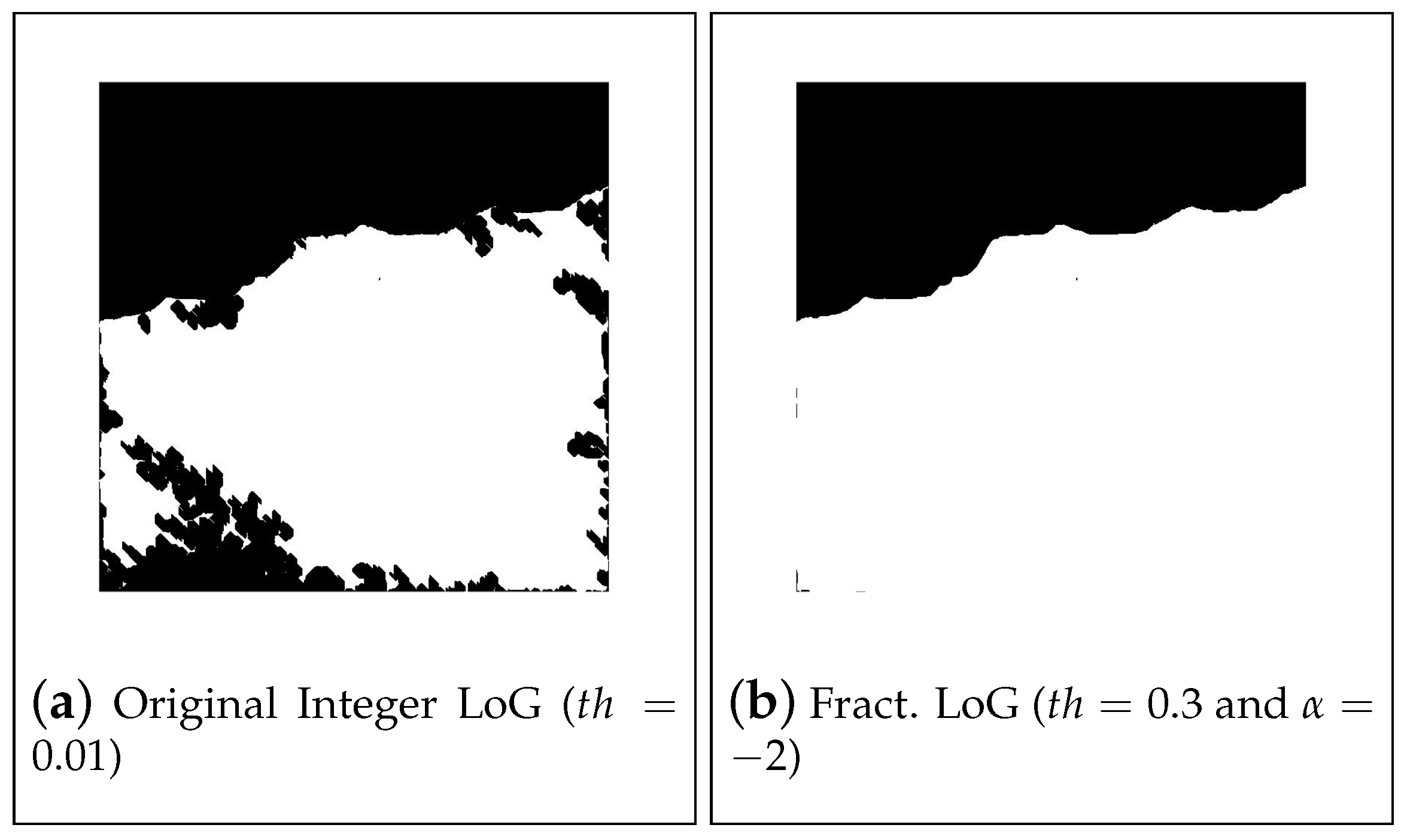
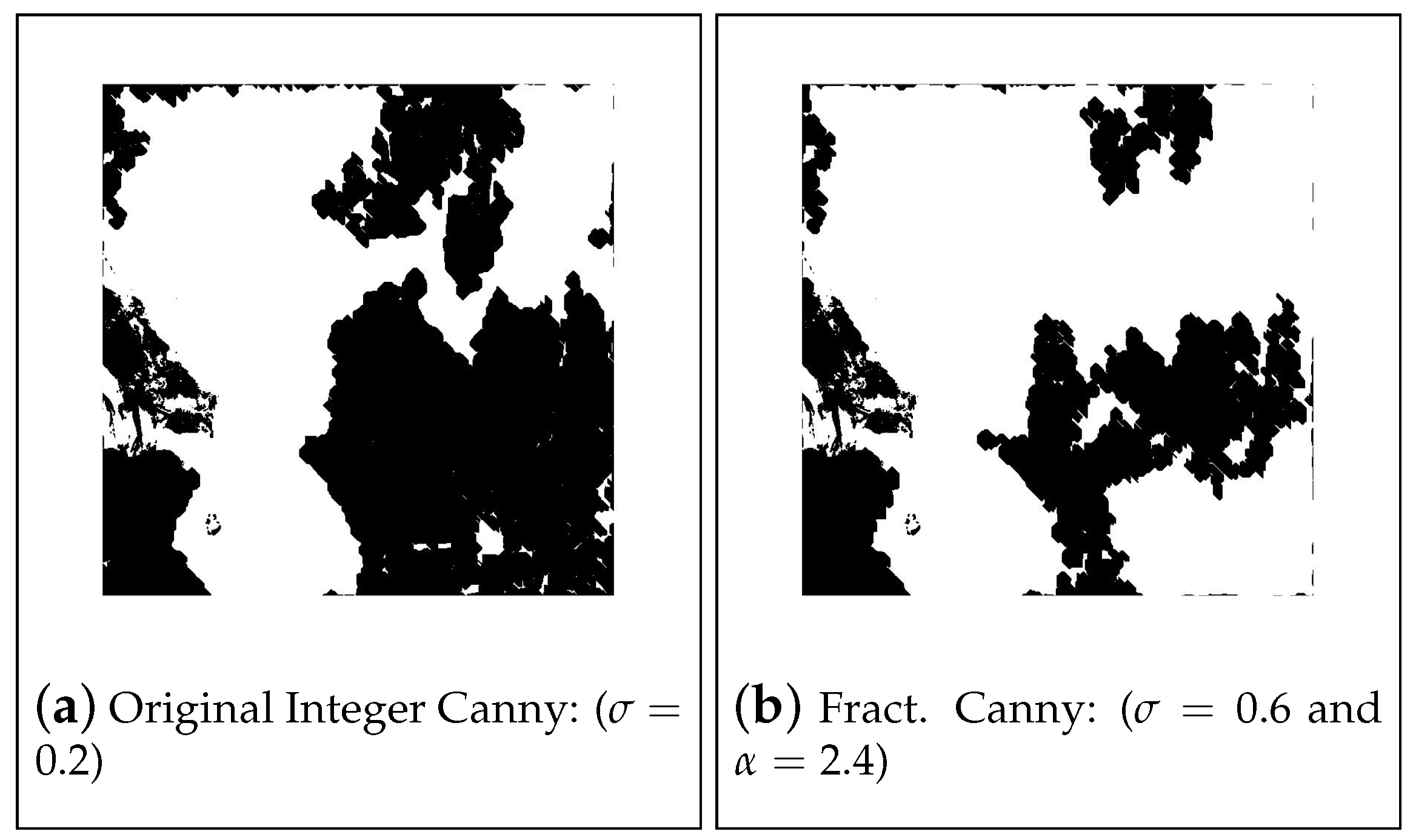
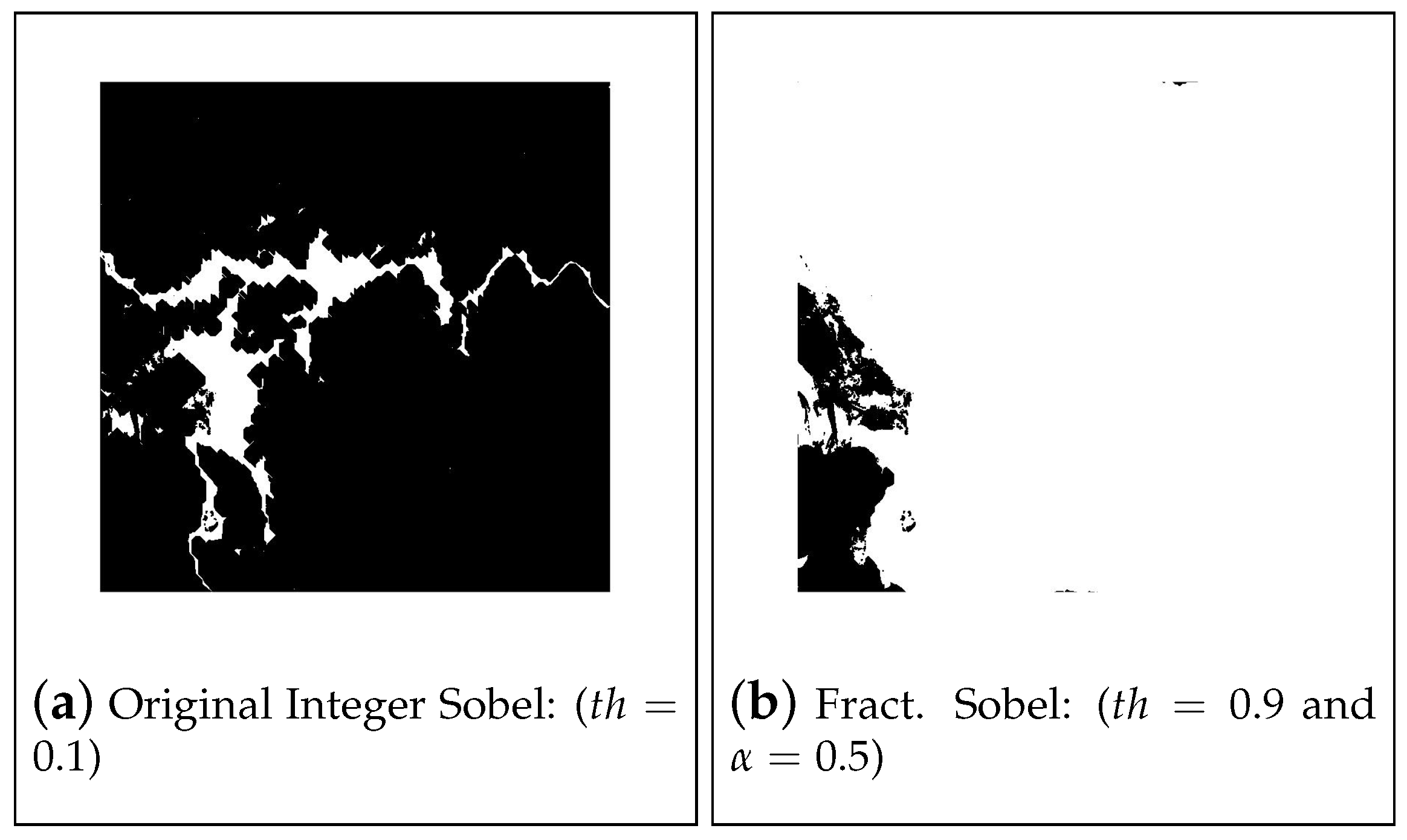
The first step of performance analysis is to understand, in each edge detection algorithm, if its fractional order based adaptation outperforms the conventional integer version. Therefore, all the algorithms formulated in Section 2 were tested. The performance was evaluated for all 43 images in the database, converted for simplicity purposes to grey-scale, and using the metrics introduced in Section 3.1. The best performances of the different detectors for the selected images are presented in Figure 8, Figure 9, Figure 10, Figure 11, Figure 12, Figure 13, Figure 14, Figure 15, Figure 16, Figure 17, Figure 18, Figure 19, Figure 20, Figure 21, Figure 22 and Figure 23 and Table 2, Table 3, Table 4 and Table 5.
3.3. Grey-Scale Edge Detectors vs. Color Based Edge Detectors
As explained before, color edge detection algorithms were implemented and tested with the whole data set due to their good results in other applications. All the six methods were adapted and applied in the main algorithm in order to perform color-based edge detection. The best results of the performance assessment for these versions of the algorithms are presented above and are compared with the corresponding best grey-scale result, using index :
The results of this comparison are presented under the form of histograms (in semilogarithmic plots) for each detector in Figure 24.
3.4. Overall Performance with Varying Parameters
3.5. Overall Performance with Fixed Parameters
One crucial objective of this work is to assess if it is possible to find and easily tune parameters, in an automatic way, without loosing performance. A search for optimal fixed parameters was conducted sorting performance results using fixed parameters for all the images in the data set. Table 7 and Figure 26 present the best fixed parameters results for each detector; they are discussed in the next section.
4. Discussion and Conclusions
In this paper, an automatic coasts edge detection tool using five state-of-the-art edge detection versions and seven novel detector versions was presented. The conventional integer versions of the algorithms were also tested and compared to fractional solutions.
Forty-three high definition (10,980p × 10,980p) satellite images were tested using the different versions of the operators in a wide range of parameters.
The grey-scale Fractional Derivatives operator was the detector that provided the best average scores regarding all figures, with varying parameters. The mean Jaccard coefficient for this operator was 0.9623, i.e. the algorithm identified correctly in average 96.23% of the pixels in the input images.
In remote sensing, it is important not only that the algorithm can reach high efficiency but also that the parameters required are possible to implement for an automatic solution. Despite the exceptional performance achieved with varying parameters, this Jaccard coefficient is only possible using a great spread of parameters impossible to reach in automatic solutions. Thus, the search for a solution with fixed parameters was conducted. In this case, the color-based Fractional Derivatives operator was the method that provided the best average scores regarding all figures in the data set, with a Jaccard metric of 0.9436. The result obtained sets a fixed-parameter solution that allows automatic detection of coasts with a decrease in performance compared to the aforementioned varying-parameters of less than 2%.
Further analyzing overall performance Table 6 and Table 7, as well as the performance data in [20], one may draw a few more conclusions. The usage of fractional derivatives in edge detection for this application matched or improved, in most cases, the performance of the conventional integer methods, which is not surprising since more information is available to be used. The color based algorithms allowed to equal or improve the performance of grey-scale methods in most cases. However, often the increase in performance is low in percentage. Nevertheless, and since we are dealing with images that are composed of more than 120 million pixels, a percentage of 1% increase corresponds to more than 1 million pixels correctly identified.
To summarize, in this study a successful automatic tool was developed that identifies and segments coasts in satellite images using both grey-scale and novel color-based fractional edge detectors. Subsequent parameters that allow the automation of this tool were also found.
Author Contributions
M.H.: methodology, software, investigation, data curation, writing – original draft preparation, visualization; D.V.: conceptualization, methodology, validation, investigation, writing – review and editing, supervision; R.M.: conceptualization, methodology, validation, investigation, data curation, writing – review and editing, supervision. All authors have read and agreed to the published version of the manuscript.
Funding
This research received no external funding.
Institutional Review Board Statement
Not applicable.
Informed Consent Statement
Not applicable.
Data Availability Statement
See [20].
Acknowledgments
This work was supported by FCT, through IDMEC, under LAETA, project UIDB/50022/2020; and by FCT under the ICT (Institute of Earth Sciences) project UIDB/04683/2020. The authors would like to acknowledge ESA, Copernicus for kindly providing access to the database for this research.
Conflicts of Interest
The authors declare no conflict of interest.
References
- ESA. Sentinel-2. 2020. Available online: https://sentinel.esa.int/web/sentinel/missions/sentinel-2/mission-objectives (accessed on 12 June 2020).
- Yang, Q.; Chen, D.; Zhao, T.; Chen, Y. Fractional calculus in image processing: A review. Fract. Calc. Appl. Anal. 2016, 19, 1222–1249. [Google Scholar] [CrossRef] [Green Version]
- Kanade, T.; Shafer, S. Image Understanding Research at Carnegie Mellon. In Proceedings of the Workshop on Image Understanding Workshop, December 1989; Morgan Kaufmann Publishers Inc.: San Francisco, CA, USA, 1989; pp. 32–48. [Google Scholar]
- Cumani, A. Edge detection in multispectral images. CVGIP Graph. Model. Image Process. 1991, 53, 40–51. [Google Scholar] [CrossRef]
- Henriques, M.; Valério, D.; Gordo, P.; Melicio, R. Fractional Order Colour Image Processing. Mathematics 2021, 9, 457. [Google Scholar] [CrossRef]
- Bento, T.; Valério, D.; Teodoro, P.; Martins, J. Fractional order image processing of medical images. J. Appl. Nonlinear Dyn. 2017, 6, 181–191. [Google Scholar] [CrossRef]
- Valério, D.; Sá da Costa, J. An Introduction to Fractional Control; IET: Stevenage, UK, 2013; ISBN 978-1-84919-545-4. [Google Scholar]
- Samko, S.G.; Kilbas, A.A.; Marichev, O.I. Fractional Integrals and Derivatives; Gordon and Breach: Yverdon, Switzerland, 1993. [Google Scholar]
- Ortigueira, M.D.; Valério, D. Fractional Signals and Systems; De Gruyter: Berlin, Germany, 2020. [Google Scholar]
- Mathieu, B.; Melchior, P.; Oustaloup, A.; Ceyral, C. Fractional differentiation for edge detection. Signal Process. 2003, 83, 2421–2432. [Google Scholar] [CrossRef]
- Chen, X.; Fei, X. Improving Edge-Detection Algorithm Based on Fractional Differential Approach; IPCSIT: Singapore, 2012; Volume 50, Available online: http://www.ipcsit.com/vol50/048-ICIVC2012-S0064.pdf (accessed on 4 June 2021).
- Tian, D.; Wu, J.; Yang, Y. A fractional-order edge detection operator for medical image structure feature extraction. In Proceedings of the 26th Chinese Control and Decision Conference, CCDC, Changsha, China, 31 May–2 June 2014. [Google Scholar] [CrossRef]
- Yaacoub, C.; Zeid Daou, R.A. Fractional Order Sobel Edge Detector. In Proceedings of the 2019 Ninth International Conference on Image Processing Theory, Tools and Applications (IPTA), Istanbul, Turkey, 6–9 November 2019; pp. 1–5. [Google Scholar] [CrossRef]
- Tian, D.; Wu, J.; Yang, Y. A Fractional-Order Laplacian Operator for Image Edge Detection. Appl. Mech. Mater. 2014, 536–537, 55–58. [Google Scholar] [CrossRef]
- Sohail, A.; Bég, O.A.; Li, Z.; Celik, S. Physics of fractional imaging in biomedicine. Prog. Biophys. Mol. Biol. 2018, 140, 13–20. [Google Scholar] [CrossRef] [PubMed]
- Yu, Q.; Vegh, V.; Liu, F.; Turner, I. A Variable Order Fractional Differential-Based Texture Enhancement Algorithm with Application in Medical Imaging. PLoS ONE 2015, 10, e0132952. [Google Scholar] [CrossRef] [PubMed] [Green Version]
- Babbar, J.; Rathee, N. Satellite Image Analysis: A Review. In Proceedings of the IEEE International Conference on Electronics, Communication and Computing Technologies (ICECCT), Coimbatore, India, 20–22 February 2019. [Google Scholar] [CrossRef]
- Dshmukh, K.; Badole, M. A Review Article of Satellite Image Different Type Approach. Int. J. Sci. Res. 2017, 6, 941–944. [Google Scholar]
- ESA. Copernicus Open Access Hub. 2020. Available online: https://scihub.copernicus.eu/ (accessed on 31 March 2020).
- Henriques, M. Results Repository. 2020. Available online: https://drive.google.com/drive/folders/1GMeKvc3oqNWfzd4h-GyRwHT9yFJ_UDLP?usp=sharing (accessed on 4 June 2021).
- Valério, D.; da Costa, J.S. Introduction to single-input, single-output fractional control. IET Control Theory Appl. 2011, 5, 1033–1057. [Google Scholar] [CrossRef]
- Canny, J. A computational approach to edge detection. IEEE Trans. Pattern Anal. Mach. Intell. 1986, 679–698. [Google Scholar] [CrossRef]
- Fisher, R.; Perkins, S.; Walker, A.; Wolfart, E. Image Processing Learning Resources. 2004. Available online: http://homepages.inf.ed.ac.uk/rbf/HIPR2/hipr_top.htm (accessed on 30 July 2020).
- Roberts, L. Machine Perception of 3-D Solids. Ph.D. Thesis, Massachusetts Institute of Technology, Cambridge, MA, USA, 1963. [Google Scholar]
- Zhu, S.Y.; Plataniotis, K.N.; Venetsanopoulos, A.N. Comprehensive analysis of edge detection in color image processing. Opt. Eng. 1999, 38, 612–625. [Google Scholar] [CrossRef]
Figure 1.
Image number 12 to be evaluated with corresponding ground truth.

Figure 2.
Image number 18 to be evaluated with corresponding ground truth.

Figure 3.
Image number 27 to be evaluated with corresponding ground truth.

Figure 4.
Image number 38 to be evaluated with corresponding ground truth.

Figure 5.
Original image and Blue Mask of Coast_D(23).jpg.

Figure 6.
Output of an edge detection operation.

Figure 7.
Totally Processed Image.

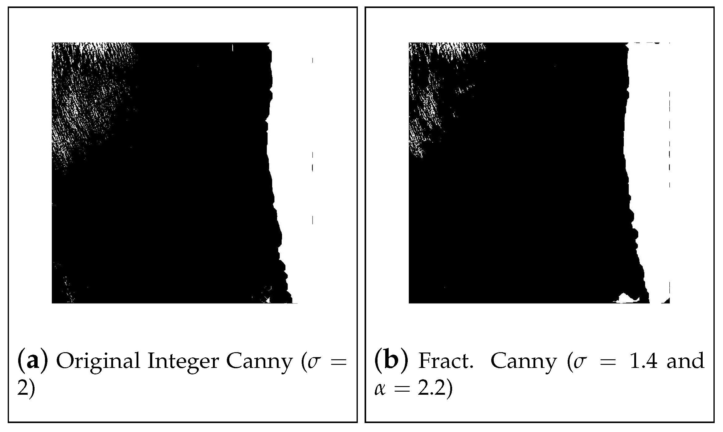
Figure 8.
Best results for image 12 processed using Canny algorithms.

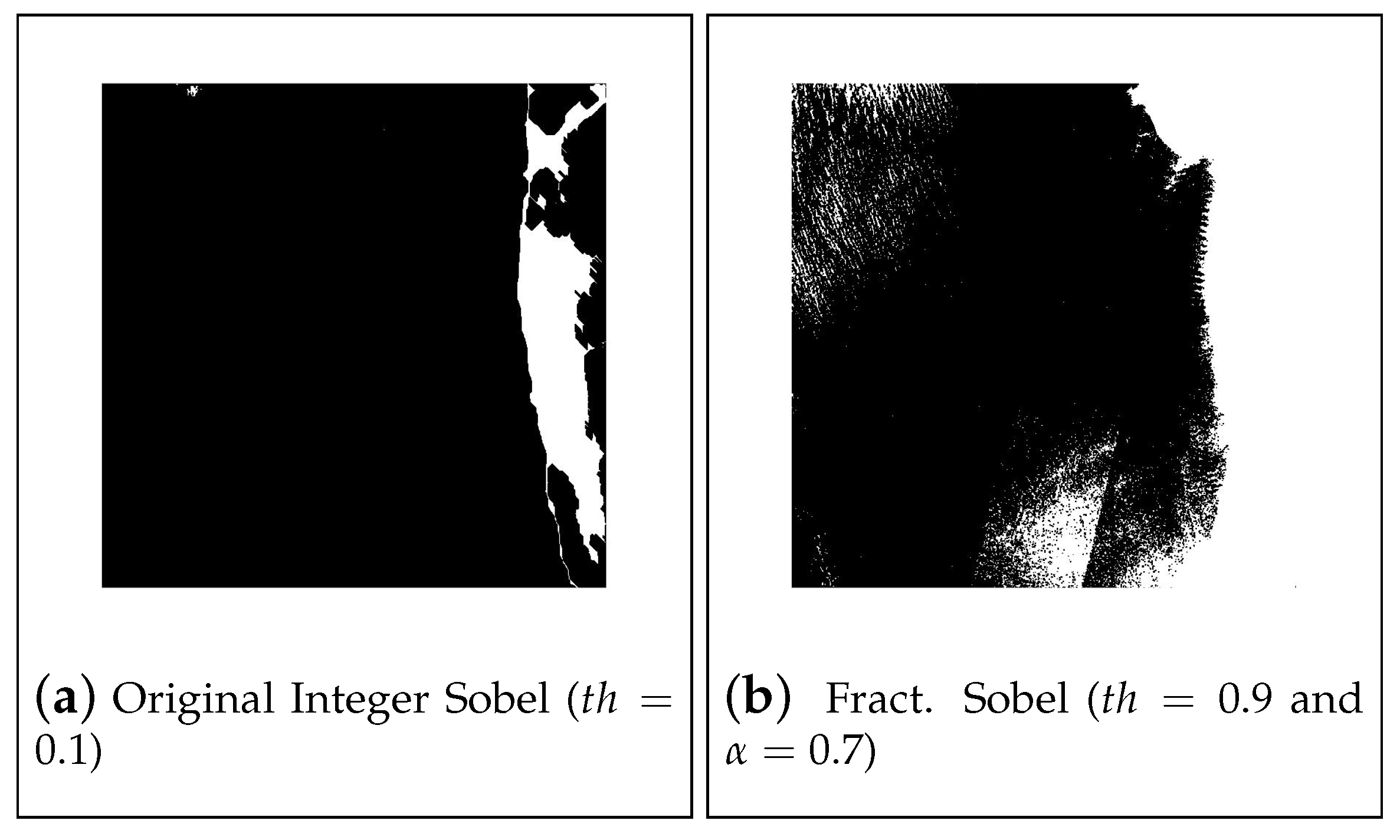
Figure 9.
Best results for image 12 processed using Sobel algorithms.

Figure 10.
Best results for image 12 processed using Roberts algorithms.

Figure 11.
Best results for image 12 processed using LoG algorithms.

Figure 12.
Best results for image 18 processed using Canny algorithms.

Figure 13.
Best results for image 18 processed using Sobel algorithms.

Figure 14.
Best results for image 18 processed using Roberts algorithms.

Figure 15.
Best results for image 18 processed using LoG algorithms.

Figure 16.
Best results for image 27 processed using Canny algorithms.

Figure 17.
Best results for image 27 processed using Sobel algorithms.

Figure 18.
Best results for image 27 processed using Roberts algorithms.

Figure 19.
Best results for image 27 processed using LoG algorithms.

Figure 20.
Best results for image 38 processed using Canny algorithms.

Figure 21.
Best results for image 38 processed using Sobel algorithms.

Figure 22.
Best results for image 38 processed using Roberts algorithms.

Figure 23.
Best results for image 38 processed using LoG algorithms.

Figure 24.
Analysis of performance comparison between grey-scale and color based detectors.

Figure 25.
Bar chart with best results average for all images (Varying parameters).

Figure 26.
Bar chart with best results average for all images (Fixed parameters).


Table 1.
Performance Instances.
| Processed Image | ||||
|---|---|---|---|---|
| 0 | 1 | |||
| Ground Truth | 0 | TN | FP | |
| 1 | FN | TP | ||
Table 2.
Best performance results using Grey-Scale detectors on image 12.
| Método | Threshold | J | D | Sensitivity | Specificity | ||
|---|---|---|---|---|---|---|---|
| Integer Canny | 2.0 | - | - | 0.8685 | 0.9296 | 0.9960 | 0.9758 |
| Fractional Canny | 1.4 | - | 2.2 | 0.8885 | 0.9410 | 0.9945 | 0.9804 |
| Integer Sobel | - | 0.1 | - | 0.5043 | 0.6705 | 0.5104 | 0.9758 |
| Fractional Sobel | - | 0.9 | 0.7 | 0.5620 | 0.7196 | 0.9999 | 0.8717 |
| Integer Roberts | - | 0.1 | - | 0.4440 | 0.6149 | 0.4486 | 0.9983 |
| Fractional Roberts | - | 0.1 | 0.8 | 0.9245 | 0.9608 | 0.9595 | 0.9938 |
| Integer LoG | - | 0.01 | - | 0.5737 | 0.7291 | 0.5820 | 0.9976 |
| Fractional LoG | - | 0.3 | 0.9480 | 0.9733 | 0.9718 | 0.9959 |
Table 3.
Best performance results using Grey-Scale detectors on image 18.
| Método | Threshold | J | D | Sensitivity | Specificity | ||
|---|---|---|---|---|---|---|---|
| Integer Canny | 1.6 | - | - | 0.6598 | 0.7950 | 0.6767 | 0.9914 |
| Fractional Canny | 1.8 | - | 0.6600 | 0.7952 | 0.6741 | 0.9928 | |
| Integer Sobel | - | 0.1 | - | 0.1419 | 0.2486 | 0.1445 | 0.9940 |
| Fractional Sobel | - | 0.9 | 0.6 | 0.6600 | 0.7952 | 0.6741 | 0.9928 |
| Integer Roberts | - | 0.1 | - | 0.1589 | 0.2742 | 0.1619 | 0.9934 |
| Fractional Roberts | - | 0.1 | 0.6588 | 0.7943 | 0.6771 | 0.9907 | |
| Integer LoG | - | 0.01 | - | 0.1051 | 0.1902 | 0.1065 | 0.9957 |
| Fractional LoG | - | 0.3 | 3.0 | 0.6594 | 0.7948 | 0.6771 | 0.9910 |
Table 4.
Best performance results using Grey-Scale detectors on image 27.
| Método | Threshold | J | D | Sensitivity | Specificity | ||
|---|---|---|---|---|---|---|---|
| Integer Canny | 0.8 | - | - | 0.9952 | 0.9976 | 0.9986 | 0.9932 |
| Fractional Canny | 0.6 | - | 2.6 | 0.9956 | 0.9978 | 0.9984 | 0.9943 |
| Integer Sobel | - | 0.8 | - | 0.9952 | 0.9976 | 0.9986 | 0.9932 |
| Fractional Sobel | - | 0.9 | 1.4 | 0.9948 | 0.9974 | 0.9987 | 0.9919 |
| Integer Roberts | - | 0.1 | - | 0.8614 | 0.9255 | 0.8618 | 0.9990 |
| Fractional Roberts | - | 0.1 | 2.4 | 0.9952 | 0.9976 | 0.9981 | 0.9940 |
| Integer LoG | - | 0.01 | - | 0.8321 | 0.9084 | 0.8326 | 0.9988 |
| Fractional LoG | - | 0.1 | 0.9957 | 0.9978 | 0.9982 | 0.9950 |
Table 5.
Best performance results using Grey-Scale detectors on image 38.
| Method | k | Threshold | J | D | Sensitivity | Specificity | ||
|---|---|---|---|---|---|---|---|---|
| Integer Canny | - | 0.2 | - | - | 0.5180 | 0.6825 | 0.5365 | 0.7167 |
| Fractional Canny | - | 0.6 | - | 2.4 | 0.7356 | 0.8477 | 0.7600 | 0.7359 |
| Integer Sobel | - | - | 0.1 | - | 0.0768 | 0.1427 | 0.0775 | 0.9271 |
| Fractional Sobel | - | - | 0.9 | 0.5 | 0.9600 | 0.9796 | 0.9997 | 0.6710 |
| Integer Roberts | - | - | 0.1 | - | 0.0618 | 0.1163 | 0.0622 | 0.9451 |
| Fractional Roberts | - | - | 0.1 | 0.9613 | 0.9803 | 0.9990 | 0.6877 | |
| Integer LoG | - | - | 0.01 | - | 0.0887 | 0.1630 | 0.0898 | 0.9076 |
| Fractional LoG | - | - | 0.1 | 1.8 | 0.9637 | 0.9815 | 0.9994 | 0.7046 |
| CRONE | 2 | - | - | 3 | 0.9612 | 0.9802 | 0.9995 | 0.6818 |
| Fract. Deriv. Mask | - | - | 0.9 | 2.3 | 0.9625 | 0.9809 | 0.9995 | 0.6936 |
Table 6.
Ranking of the best results average for all images.
| Detector | |
|---|---|
| Fractional Derivative Op. | 0.9623 |
| Color Fractional Derivative Op. | 0.9596 |
| Color Laplacian of Gaussian | 0.9554 |
| Color Roberts | 0.9537 |
| Laplacian of Gaussian | 0.9531 |
| Color Sobel | 0.9478 |
| Roberts | 0.9474 |
| Color CRONE | 0.9461 |
| Color Canny | 0.9448 |
| CRONE | 0.9447 |
| Canny | 0.9342 |
| Sobel | 0.9282 |
Table 7.
Full volume analysis of best results with fixed parameters for all detectors.
| Detector | k | ||||
|---|---|---|---|---|---|
| Color Fractional Derivative Op. | 0.9 | - | - | 0.8 | 0.9436 |
| Fractional Derivative Op. | 0.7 | - | - | 0.8 | 0.9428 |
| Color CRONE | - | 5 | - | 0.9 | 0.9328 |
| CRONE | - | 5 | - | 1.1 | 0.9261 |
| Color Canny | - | - | 0.7 | 1.7 | 0.9193 |
| Color Roberts | 0.1 | - | - | 1.4 | 0.9174 |
| Color Sobel | 0.3 | - | - | −0.2 | 0.9153 |
| Sobel | 0.9 | - | - | 0.2 | 0.9111 |
| Color Laplacian of Gaussian | 0.1 | - | - | −0.9 | 0.9108 |
| Roberts | 0.1 | - | - | −1.3 | 0.9076 |
| Laplacian of Gaussian | 0.1 | - | - | −1.4 | 0.9028 |
| Canny | - | - | 0.6 | 0 | 0.9011 |
Publisher’s Note: MDPI stays neutral with regard to jurisdictional claims in published maps and institutional affiliations. |
© 2021 by the authors. Licensee MDPI, Basel, Switzerland. This article is an open access article distributed under the terms and conditions of the Creative Commons Attribution (CC BY) license (https://creativecommons.org/licenses/by/4.0/).
Share and Cite
MDPI and ACS Style
Henriques, M.; Valério, D.; Melicio, R. Fractional Order Processing of Satellite Images. Appl. Sci. 2021, 11, 5288. https://0-doi-org.brum.beds.ac.uk/10.3390/app11115288
AMA Style
Henriques M, Valério D, Melicio R. Fractional Order Processing of Satellite Images. Applied Sciences. 2021; 11(11):5288. https://0-doi-org.brum.beds.ac.uk/10.3390/app11115288
Chicago/Turabian StyleHenriques, Manuel, Duarte Valério, and Rui Melicio. 2021. "Fractional Order Processing of Satellite Images" Applied Sciences 11, no. 11: 5288. https://0-doi-org.brum.beds.ac.uk/10.3390/app11115288
Note that from the first issue of 2016, this journal uses article numbers instead of page numbers. See further details here.