Variable Neighborhood Strategy Adaptive Search to Solve Parallel-Machine Scheduling to Minimize Energy Consumption While Considering Job Priority and Control Makespan

Abstract

Environmental concerns and rising energy prices put great pressure on the manufacturing industry to reduce pollution and save energy. Electricity is one of the main machinery energy sources in a plant; thus, reducing energy consumption both saves energy costs and protects our planet. This paper proposes the novel method called variable neighborhood strategy adaptive search (VaNSAS) in order to minimize energy consumption while also considering job priority and makespan control for parallel-machine scheduling problems. The newly presented neighborhood strategies of (1) solution destroy and repair (SDR), (2) track-transition method (TTM), and (3) multiplier factor (MF) were proposed and tested against the original differential evaluation (DE), current practice procedure (CU), SDR, TTM, and MF for three groups of test instances, namely small, medium, and large. Experimental results revealed that VaNSAS outperformed DE, CU, SDR, TTM, and MF, as it could find the optimal solution and the mathematical model in the small test instance, while the DE could only find 25%, and the others could not. In the remaining test instances, VaNSAS performed 16.35–19.55% better than the best solution obtained from Lingo, followed by DE, CU, SDR, TTM, and MF, which performed 7.89–14.59% better. Unfortunately, the CU failed to improve the solution and had worse performance than that of Lingo, including all proposed methods.

1. Introduction

The manufacturing industry is facing a great deal of pressure with regard to saving energy and reducing emissions, since it is an energy-intensive industry. In 2020, its energy consumption reached 1443.1 trillion British thermal units (Btu), of which electricity consumption was 200.7 trillion Btu [1]. In the same year, energy-related carbon dioxide emissions by the manufacturing industry reached 1057 million metric tons [2]. Studying energy-efficiency scheduling under electricity cost is of great significance for manufacturing firms to improve their energy efficiency. In a factory, machinery is the main energy-consuming unit [3,4,5,6]. Reducing machine energy consumption economically and environmentally improves sustainable manufacturing. There are many potential energy-reduction approaches in a manufacturing plant, such as developing more energy-efficient machines and processes. In the production line, production planning and scheduling generally impact energy efficiency. Energy efficiency can also be increased by the suitable utilization of machines in the shop floor [6,7,8,9,10,11,12]. In the production process, the electricity consumption of each job is sometimes different, indicating that an operation with high electricity consumption is arranged for low processing time jobs, and an operation with low electricity consumption is arranged for high processing time jobs, so that the electricity cost can be decreased [5,6,13]. Paying too much attention to energy cost as an outstanding optimization objective may cause a long makespan and imbalanced workload on machines, as well as lead to bottlenecks, late deliveries, and even untimely machine failure [14,15,16,17].

Production scheduling is explicitly important in a modern manufactory, consisting of planning and sequencing jobs into machines, since mass production heavily relies on a large number of machines working in parallel. Parallel machines can process several jobs simultaneously without affecting each other. Parallel machine scheduling is defined as sequencing and assigning jobs into machines when similar types of machines are available and jobs can be scheduled in these machines. A variety of sequencing and/or processing restrictions often exist when decision makers try to minimize some related objective functions [14,15,16,17,18,19,20,21,22,23,24]; however, most enterprises still use advanced machines running alongside outdated ones. In contrast to the old ones, modern machines are usually adjusted to work at a high speed and save energy. Speeding up old machines to operate as fast as modern ones results in them consuming more electric power and releasing more pollutants [25]. Sequencing and assigning jobs to a particular machine that can process different jobs at different production rates is considered to be the parallel-machine-scheduling problem. Solutions or algorithms constructed to schedule parallel machines are important because, when implemented in all sorts of parallel-machine problems, they can obtain good solutions for the overall production-planning process in a factory [18,19].

Although most scheduling problems consider production efficiency, cost, and quality as optimization problems, considering the costs of energy and gas emissions—known as the green scheduling problem—has attracted the attention of researchers [9,10,11,14,25]. In addition, various constraints have been addressed in parallel-machine-scheduling problems, such as setup time, machine-available time, ready time, release date, due date, and delivery time [14,26]. In this study, the due-date constraint was considered with makespan control, since late-delivery cost and production-overhead cost per working hour may be a thorny issue for entrepreneurs. Therefore, job priority and makespan control should be seriously considered for production planning as well. On the basis of the above discussion, many scholars and manufacturing firms should be aware of the importance of energy-efficiency and job-priority concerns, on top of minimizing the makespan. There are a few studies on the parallel-machine-scheduling problem with a concept of energy consumption that consider job priority and makespan control. Therefore, this addressed scheduling is both an objective optimization problem and an NP-hard problem. The differential evolutionary (DE) algorithm is suitable to solve this kind of problem because it can obtain non-dominated solutions in a single run and has been successfully applied to optimization problems [17,20,24,27,28,29]. In addition, metaheuristics based on local search methods, such as the variable neighborhood strategies adaptive search (VaNSAS), have been successfully applied to solve many combinatorial optimizations problems [30,31,32,33,34,35,36,37,38,39,40], which inspired us to develop a parallel-machine-scheduling model, and to propose VaNSAS and new neighborhood strategies: (1) solution destroy and repair (SDR); (2) track-transition method (TTM); and (3) multiplier factor (MF).

Nowadays, the cost of energy consumption is key in terms of production efficiency and environmental sustainability for industrial firms. A significant amount of research has been done on parallel-machine-scheduling problems that are strongly NP-hard. We refer to Chen [41], Pinedo [42] and Behera [43] for the discussion on the complexity of parallel-machine scheduling. Therefore, this study investigates the parallel-machine-scheduling problem for minimizing energy consumption while considering job priority and makespan control. In order to obtain the near Pareto front, we developed VaNSAS: (1) solution destroy and repair (SDR); (2) the track-transition method (TTM); and (3) multiplier factor (MF). On the basis of the problem characteristic and evolutionary algorithm, the proposed VaNSAS uses a new encode scheme that can convert discrete optimization problems into continuous optimization problems, and applies VaNSAS with three different techniques to further improve quality.

The remainder of the study is organized as follows: Section 2 reviews the literature related to parallel scheduling, considering energy consumption, job priority, and makespan control, including DE and VaNSAS applications; Section 3 describes a formal definition of the addressed problem and a mathematical model for the proposed problem; Section 4 describes the proposed VaNSAS, SDR, TTM, and MF with multiple operators in order to handle the scheduling problem; Section 5 presents and analyzes the experiment results of our proposed VaNSAS, SDR, TTM, and MF; Section 6 provides the conclusion and suggestions for future studies.

2. Literature Review

Environmental and sustainable energy is a critical topic. CO₂ emissions into the atmosphere are strongly related to energy consumption in human activities; they are generated by traditional fuels from natural resources which are becoming depleted [44]. Liu [39] studied scheduling problems that were related to an environment where the objective of minimizing CO₂ emissions was investigated with total weighted tardiness (TWT). The non-dominated sorting-based genetic algorithm II (NSGA-II) and the ε-archived genetic algorithm (ε-AGA) were presented to solve two batch-scheduling problems. In their subsequent article, Liu and Huang [10] demonstrated both the effectiveness of an adaptive multi-objective genetic algorithm (AMGA) in finding the Pareto optimal set, and the efficiency of NSGA-II in bicriterion scheduling on a batch-processing machine with dynamic job arrivals. Regarding low carbon emissions in the parallel-machine-scheduling problem, Pan et al. [40] introduced the advantages of a novel imperialist competitive algorithm (ICA) to minimize total tardiness, total energy consumption, and CO₂ emissions.

Various energy concerns (e.g., energy consumption, energy efficiency, carbon footprint, and energy cost) are investigated in production-scheduling problems. There are also several studies on energy-efficient production systems. For example, Mouzon et al. [45] improved product operation methods, such as several dispatching rules and mathematical programming, in order to minimize the total completion time and energy consumption of manufacturing equipment in production-scheduling problems. Angel et al. [46] introduced a randomized approximation algorithm for the problem of energy-consumption scheduling for unrelated parallel machines with the average weighted completion time. Sobottka et al. [47] demonstrated the development and evaluation of a digital method for multi-objective optimization problems considering traditional business aims and energy efficiency in a metal-casting manufactory. The improved method, including hybrid simulation-based multi-criterion optimization as a multi-stage hybrid heuristic and metaheuristic method, was employed in a heat-treatment process, which requires order batching and sequencing on parallel machines under complex restrictions.

In the context of energy cost, a number of works attempted to reduce it during production when energy and electricity prices vary with time of use. For example, Fang et al. [7] proposed a mixed integer programming model for optimizing the operating schedule of a flow shop considering both productivity- and energy-related criteria. Zeng [23] studied the uniform parallel-machine-scheduling problem with electricity cost and time-dependent or time-of-use electricity tariffs, where electricity price changes by the working hour within a day. Firstly, a bi-objective mixed-integer linear-programming model was constructed for this problem. Then, the proposed method (an insertion algorithm) was applied to minimize total electricity cost and the number of operated machines. Zhou et al. [19] presented a multi-objective differential evolution algorithm to solve the parallel-batch-processing machine-scheduling problem (BPM) in the presence of dynamic job arrivals and a time-of-use pricing scheme. The objective was to simultaneously minimize makespan and minimize total electricity cost (TEC). Recently, Nanthapodej et al. [48] introduced the hybrid differential devolution algorithm and adaptive large neighborhood search, and demonstrated a superior performance in finding high quality solutions within a short computation time of the proposed algorithm for solving the parallel-machine-scheduling problem, with minimizing total energy cost (TEC) as key for environmental sustainability, and controlling machine load balance as an indicator of production efficiency.

Although more attention is now paid to energy cost in parallel-machine-scheduling problems, some constraints for job priority and makespan control are also important, such as starting time, completion time, due date, and delivery time, since late-delivery cost and production-overhead cost per working hour impact manufacturers. Some studies attempted to avoid late- or express-delivery charges, such as lateness and tardiness issues. For instance, Chaudhry et al. [49] considered the minimization of total tardiness in identical parallel-machine-scheduling problems by using a genetic algorithm (GA), and compared it with branch-and-bound and particle-swarm-optimization methods. Then, Pei et al. [50] demonstrated minimizing maximal earliness and number of tardy jobs in parallel-machine-scheduling problems. That article proposed the hybrid variable neighborhood search (VNS)–gravitational search algorithm (GSA), which is a combination of VNS and GSA to find a solution. Solution-search efficiency is also an attractive goal for many studies. Maecker and Shen [51] also applied the VNS algorithm with the fast evaluation technique (FET) to improve the computational efficiency of solution finding in the identical parallel-machine problem with machine-dependent delivery times in order to minimize total weighted tardiness.

In a continuous search space for function optimization, differential evolution (DE) is a type of evolutionary algorithm that is widely implemented [27]. The DE algorithm has gained much attention from scholars since it was first presented by Storn and Price [28]. There are a variety of DE algorithms in industrial applications studied for optimization problems. For instance, the DE algorithm was implemented for solving production-scheduling problems. Wang et al. [29] demonstrated hybrid differential evolution (HDE) in scheduling problems with splitting jobs. The study proposed a global search method with block mutation and block crossover. Experiment results revealed that the proposed HDE performed better than the traditional DE did. Zhou et al. [52] showed the performance of the hybrid DE algorithm for the uniform parallel-machine-scheduling problem with arbitrary job sizes, non-identical capacities, and different speeds. The objective was to minimize makespan. The HDE algorithm was proposed for solving large-scale problems. In this algorithm, individuals were represented as a discrete job sequence. The proposed algorithm and novel mutation were designed on the basis of this representative. Wu and Che [53] proposed a memetic differential evolution algorithm for an energy-efficient bi-objective-unrelated parallel-machine-scheduling problem in order to minimize makespan and total energy consumption. Efficient speed adjusting and job machine swap heuristic were introduced and integrated into the algorithm as a local search method with an adaptive meta-Lamarckian learning strategy. Zhou et al. [19] presented a multi-objective DE algorithm for effectively solving the parallel-batch-processing machine-scheduling problem while considering energy cost on a large scale. In this algorithm, individuals were encoded into job permutations and discrete mutations; crossover operators were designed on the basis of the encoding structure, and a Pareto selection operator was proposed to select what the individuals for the next population are. Defining job permutation, a heuristic was employed to group jobs into batches and schedule them on BPMs.

In addition, a procedure to minimize the total energy cost of a schedule without compromising the makespan was proposed by Li et al. [54]. They investigated the parallel-machine-scheduling problem with different-colored families, sequence-dependent setup times, and machine-eligibility restriction of the dyeing process in textile manufacturing. Generally, the dyeing optimization problem is NP-hard, and the HDE algorithm was proposed to solve real-world data problems. The proposed HDE algorithm, a special encoding and decoding scheme, was constructed to deal with the machine-eligibility constraint, and chaos theory was applied to determine the parameter settings of the DE algorithm. Kusoncum et al. [17] presented the traditional DE with embedded heuristics to obtain near-optimal solutions in realistically sized machine scheduling, including capacitated machine restrictions and sequencing-independent setup-time considerations. Results revealed that the proposed method’s performance tended to find a new optimal solution during the simulation, while the local-search-based heuristics were trapped at some local optima, and the DE was insufficient for search intensification.

Variable neighborhood strategies adaptive search (VaNSAS) is a new type of metaheuristics that was first introduced by Theeraviriya et al. [36], with the concept of solving combinatorial optimization problems. The primary idea of the VaNSAS is to allow for algorithms to search in many different areas to obtain the best possible solution by using several searching methods. VaNSAS is very flexible to use in many optimization problems, such as the location and routing problem (LRP). Theeraviriya et al. [36] studied the LRP in the Thai rubber industry, and proposed VaNSAS to solve the problem with the objective function of fuel-cost minimization, including a realistic constraint that allowed for a vehicle to collect products by visiting rubber farms more than once in cases where they had more rubber than vehicle capacity. Computation results showed that VaNSAS could find solutions for all problem sizes in much less processing time than that needed by the exact method. After that, Pitakaso et al. [37] presented VaNSAS with another LRP, the green 2-echelon location-routing problem (G2ELRP), which is a variant of the capacitated location-routing problem (CLRP) and the 2-echelon location routing problem (2ELRP). The G2ELRP aims to reduce overall fuel consumption on the basis of distance and road conditions in both echelons. A new constraint considered in the G2ELRP is that a customer can be served more than once. The finding demonstrated that VaNSAS could solve this case and be applied to other industries.

Kusoncum et al. [17] introduced another application of VaNSAS in a sugar mill as a computational tool for scheduling sugarcane-vehicle-unloading systems. The objective was to minimize the makespan of parallel-machine-capacity scheduling with a cyclic sequence, and machine restriction included sequencing-independent setup time. Numerical results showed that, during the simulation, VaNSAS could find optimal solutions. In a manufacturing case study regarding the garment industry, the VaNSAS proposed by Jirasirilerd et al. [22] presented a better solution and less computation time in order to minimize cycle time for a simple assembly line, balancing the Type 2 problem while considering the number and types of machines operated in each workstation. Recently, Pitakaso et al. [38] applied VaNSAS to minimize the cycle time while considering the limited number of machine types in a particular workstation for the special case of the simple assembly line balancing Type 2 problems, where multi-skilled workers have a set of competencies that allow them to work on more than one machine in a workstation. Results showed that VaNSAS was able to reduce the cycle time and increase assembly line effectiveness.

The studies discussed above show that global search metaheuristics (e.g., VNS, GA, DE and VaNSAS) are effective in solving optimization problems such as parallel-machine scheduling. Due to the importance of the environmental and economic impact, studies on energy-cost concerns, job priority, and makespan control are obviously attractive and important in terms of theoretical and application value; however, no previous articles had investigated this kind of problem and employed the VaNSAS algorithm to find the solution. As a result, this paper’s objective is to minimize total energy consumption while considering job priority and makespan control for the parallel-machine-scheduling problem. In order to solve this problem, we developed a mathematical model, and introduced VaNSAS, SDR, TTM, and MF algorithms to further improve solution-search efficiency.

3. Mathematical-Model Formulation

3.1. Problem Description

This paper considers the problem of energy consumption concerning scheduling, while considering job priority and makespan control for parallel machines, to improve energy consumption and production efficiency for environmental sustainability [9]. Production costs such as overhead and late delivery are also significant and should be mentioned. Therefore, the objective of this study is to minimize total energy cost, including considering due-date and lateness constraints. In this context, a set of I different jobs {j₁, j₂, ..., j_I} were scheduled on M parallel machines {m₁, m₂, ..., m_M}. We assumed that each job j had deterministic processing time p_jm on each machine. The jobs could be assigned to any machine. Due to the job characteristics, each machine required different levels of energy consumption e_jm to process each job. All jobs were available at time zero. The completion time of job j is denoted by C_jm, which is the time when the processing of the job was completed on machine m. Only after the machine starting the process could no idle time be inserted into the schedule with no preemption. Additionally, in each time period, only one job could be processed on machine m.

On the basis of these assumptions and the following notations, a mathematical model is proposed to formulate this problem in order to minimize energy consumption while considering job priority and makespan control. This is defined as the minimization of energy-consumption, late-delivery, and production-overhead costs.

3.2. Mathematical Formulation

On the basis of the characteristics of minimizing energy consumption with job priority and makespan control for a parallel-machine-scheduling problem, the mathematical model is formulated. The details of index, parameters, decision variables, objective function, and constraints are as follows:

Index
i, j	Job indices; j, i = 1, 2,…, I when i or j = 0, 0 represents the dummy node, which is always produced first in each machine
m, n	Machine indices; m, n = 1, 2,…, M
Parameters
I	Total number of jobs
M	Total number of machines
Pjm	Processing time of job j on machine m
Ejm	Energy consumption for producing job j on machine m
Dj	Due date of job j
aj	Penalty cost of job j (priority of job)
B	Cost per time units of processing with all machines.
Ajm	Job-machine restriction; Ajm = 1 when job j can produce on machine m.
LMAX	Maximal lateness that is allowed
TMAX	Maximal number of tardy jobs that are allowed
KKK	Cost conversion for used energy
Decision Variable
Xijm	$\left\{\begin{array}{cc}1\hfill & when job i immediately produces before job j in machine m\hfill \\ 0\hfill & Otherwise \hfill \end{array}\right.$
Yjm	$\left\{\begin{array}{cc}1\hfill & when job j is assigned to machine m\hfill \\ 0\hfill & Otherwise \hfill \end{array}\right.$
Sjm	Start time of job j on machine m
Cjm	Completion time of job j on machine m
Li	Lateness of job i
Ti	$\left\{\begin{array}{cc}1\hfill & when job i delivers late \hfill \\ 0& otherwise \end{array}\right.$

Objective function

$$min Z={\displaystyle \sum }_{m=1}^M{\displaystyle \sum }_{j=1}^I{E}_{jm}{Y}_{jm}+{\displaystyle \sum }_{j=1}^I{a}_j{T}_j+{\displaystyle \sum }_{m=1}^{M}B\times Ma{x}_{j=1}^I{C}_{jm}$$

(1)

Subject to

$${{\displaystyle \sum }}_{\mathrm{j}=1}^{\mathrm{I}}{\mathrm{X}}_{0\mathrm{jm}}\le 1 \forall m$$

(2)

$${{\displaystyle \sum }}_{m=1}^M{{\displaystyle \sum }}_{i=1, i\ne j}^I{X}_{ijm}=1 \forall j$$

(3)

$${{\displaystyle \sum }}_{j=1,i\ne j}^I{X}_{ijm}\le Y_{im} \forall i, m$$

(4)

$${{\displaystyle \sum }}_{i=1,i\ne j}^I{X}_{ijm}=Y_{jm} \forall j, m$$

(5)

$${{\displaystyle \sum }}_{m=1}^M{Y}_{im}=1 \forall i$$

(6)

$$S_{jm}={{\displaystyle \sum }}_{i=1,i\ne j}^I{C}_{im}{X}_{ijm} \forall j, m$$

(7)

$$C_{jm}\ge S_{jm}+P_{jm} \forall j, m$$

(8)

$$S_{0m}=0 \forall m$$

(9)

$$C_{0m}=0 \forall m$$

(10)

$$L_i= \left\{\begin{array}{c}Ma{x}_{m=1}^M{C}_{im}-D_i if Ma{x}_{m=1}^M{C}_{im}\ge D_i\\ 0 otherwise \end{array}\right. \forall i$$

(11)

$$L_i\le L^{MAX} \forall i$$

(12)

$$T_i= \left\{\begin{array}{c}1 if L_{i }>0\\ 0 otherwise\end{array} \right. \forall i, j; i \ne j$$

(13)

$${{\displaystyle \sum }}_{i=1}^I{T}_i\le T^{MAX} \forall j, m$$

(14)

The objective function in Equation (1) attempts to minimize energy used to produce all jobs, the priority cost for jobs that deliver late, and the production-overhead cost per working hour. Equations (2) and (3) show that all jobs must be assigned to at most one machine, and the start of all assigned jobs must be Job 0 (dummy job). Equation (4) is the relationship constraint of X_ijm and Y_im. Equation (5) confirms that job i is processed before job j in machine m only when job j is assigned to machine m. Equation (6) ensures that a job can be assigned to at most one machine. Equation (7) calculates the starting time of job j in machine m, and Equation (8) is the calculation of the completion time of job j. Equations (9) and (10) define the starting and completion time of the dummy job. Equation (11) calculates the lateness of job i, while Equation (12) is used to ensure that the lateness of job i does not exceed the predefined value (L^MAX). Equation (13) decides whether job i is late, and Equation (14) ensures that the number of tardy jobs does not exceed the predefined number (T^MAX).

The mathematical model was formulated and tested on Lingo software. The optimal solution was obtained for a small problem, albeit with intolerable computation time. Solving medium or large problems desired more computation time, even for an incomplete solution. Therefore, in this study, we developed metaheuristics to solve a medium or large problem as a realistically sized problem.

4. Proposed Method

When a problem becomes larger and more complicated, solving it may not be possible by mathematical methods. Therefore, we introduced a variable neighborhood strategy adaptive search (VaNSAS), a new type of metaheuristics, which successfully improved solution-search efficiency in previous studies by adapting some VaNSAS mechanisms. This study aims to solve the parallel-machine-scheduling problem in order to minimize energy consumption with job priority and makespan control, and proposes VaNSAS for improving solution-search efficiency. The goal of VaNSAS is to allow algorithms to search for the best possible solution in different areas by using several searching methods. The solution-searching steps are to find more diversification and intensification at all times, depending on the black-box methods that were designed. The search method in VaNSAS can be a basic local search, well-known heuristics, modified metaheuristics, and a newly designed local search; therefore, VaNSAS is very flexible for applying new ideas to the algorithm and can be implemented to many optimization problems.

VaNSAS is composed of two main steps: (1) generating the initial solution (the set of tracks); and (2) performing the track-touring process. The track-touring process of VaNSAS comprises four steps: (1) the track selects the neighborhood strategy (NS); (2) the track performs the selected NS; (3) heuristic information is updated; and (4) Steps 1 to 3 are repeated until the algorithm reaches the termination condition. The overall VaNSAS processes are presented in Algorithm 1.

Algorithm 1. Variable neighborhood strategy adaptive search (VaNSAS).

Input: number of jobs, number of machines, production time, energy consumption   Output: consumed energy   Begin   Randomly generate predefined number of tracks (NT) $Z_{ijt}$   While t is less than the predefined number of iterations,   Perform track-touring process   1. Each track individually selects a black box   2. Each track performs a black-box searching process 2.1 Solution decompose and repair method (SDR) (optional) 2.2 Track-transition method (TTM) (optional) 2.3 Multiplier factor (MF) (optional)   3. t = t + 1;   End

4.1. Generating an Initial Solution

Indirect encoding was used to solve the proposed problem while we randomly generated the set of tracks.

Table 1. Example of a set of five tracks used in VaNSAS.

Track	Position	Job Elements										Machine Elements
		1	2	3	4	5	6	7	8	9	10	A	B	C
	1	0.48	0.70	0.22	0.43	0.75	0.91	0.04	0.41	0.48	0.34	0.95	0.31	0.65
	2	0.99	0.06	0.84	0.63	0.38	0.87	0.03	0.94	0.74	0.41	0.39	0.26	0.63
	3	0.04	0.49	0.62	0.44	0.13	0.49	0.59	0.32	0.97	0.44	0.02	0.52	0.01
	4	0.94	0.16	0.34	0.67	0.17	0.90	0.26	0.25	0.93	0.95	0.59	0.62	0.37
	5	0.46	0.90	0.68	0.60	0.19	0.26	0.15	0.30	0.60	0.22	0.54	0.46	0.72

shows an example of five tracks to operate in VaNSAS.

The tracks shown in Table 1 were composed of 13 positions. The first 10 positions were the track elements that represented the jobs assigned to Machines A, B, and C. We used indirect encoding, so the decoding method is essential to let the tracks reflect the real solution. The decoding method is explained as follows:

4.1.1. Decoding Methods

• Separately apply the rank order value (ROV) between job and machine vectors. The ROV of jobs is called the job sequence at position i (SJi), and machine sequence in position m is called SMm.
• Assign the first job in Position 1 of SJi to Machine 1 of SMm, assign the second job in Position 2 of Sji to the machine in Position 2 of SMm, and continuously assign the remaining jobs in position i + 1 to machine m + 1 until m = M, where M is the total number of machines. In the context of job or machine restrictions, job j is assigned to machine m only when job j is allowed to be produced on machine m. If job j is not allowed to be produced on machine m, job j is assigned to the next order of machine.
• Continue assigning jobs in position i + 1 to the machine that has minimal total processing time among all M machines until all jobs are assigned to a machine. While assigning a job to a machine, the maximal number of tardy jobs and maximal lateness must be controlled to be less than the maximal predefined number.
• Calculate completion time and energy used in Step 3.

4.1.2. Decoding-Method Example

An example value of a scheduling problem with 10 jobs and 3 machines is provided in

Table 2. Values of P_jm and E_jm for 10 jobs and 3 machines.

Job j	m	1	2	3	4	5	6	7	8	9	10
Pjm	A	22	15	30	16	29	25	26	18	26	19
	B	24	N/A	20	29	25	22	29	N/A	16	16
	C	24	16	18	22	18	N/A	17	17	18	27
Ejm	A	26	17	29	19	27	25	26	23	22	29
	B	21	N/A	30	18	25	23	30	N/A	28	26
	C	24	29	19	30	17	N/A	19	18	28	24
Dj		30	45	80	85	120	45	150	30	50	200
aj		483	421	338	449	438	480	383	321	389	418

Remarks: N/A is a job-machine restriction in which the job could not be produced on that machine.

.

P_im is the processing time of job i on machine m, and E_im is the energy consumed to produce job i on machine m. D_i is the due date of job i and a_j is penalty cost of job j.

Step 1:

Separately apply ROV to the job and machine tracks from the smallest to the largest value; results are shown in

Table 3. Track 1 before and after applying rank order value (ROV).

Track before ROV	Job/Machine	1	2	3	4	5	6	7	8	9	10	A	B	C
	Value in position	0.48	0.7	0.22	0.43	0.75	0.91	0.04	0.41	0.48	0.34	0.95	0.31	0.65
Track after ROV	Job/Machine	7	3	10	8	4	1	9	2	5	6	B	C	A
	Value in position	0.04	0.22	0.34	0.41	0.43	0.48	0.48	0.7	0.75	0.91	0.31	0.65	0.95

.

Step 2:

Apply Jobs 7, 3, and 10 to Machines B, C, and A, respectively.

Step 3:

Assign Job 8 to B, but it is not allowed to produce Job 8 on Machine B; thus, assign Job 8 to Machine C instead of Machine B. Since it has the lowest total processing time, Jobs 9, 8, 5, 6, 3, and 7 are assigned to Machines A, B, A, C, B, and B, respectively. The results of this assignment are shown in

Table 4. Results of the proposed decoding method in Step 3.

Job	7	3	10	8	4	1	9	2	5	6
Machine	B	C	A	C	B	A	B	C	A	B
Energy used (THB)	30	19	29	18	18	26	28	29	27	23

.

In this assignment, the job-production sequence of Machine B produces jobs {7, 4, 9, 6}, and Machines C and A produce jobs {3, 8, 2} and {10, 1, 5}, respectively. Then, the total energy consumption of this plan is THB 247.

Table 5. Sequence and scheduling from Table 4.

Job	10		1		5
Machine A	S10,A	C10,A	S1,A	C1,A	S5,A	C5,A
Sjm/Cjm	0	19	19	41	41	70
Dj		200		30		120
Lj		0		11		0
Tj		0		1		0
Job	7		4		9		6
Machine B	S7,B	C7,B	S4,B	C74B	S9,B	C9,B	S6,B	C6,B
Sjm/Cjm	0	29	29	58	58	76	76	98
Dj		150		85		50		45
Lj		0		0		26		53
Tj		0		0		1		1
Job	3		8		2
Machine C	S3,C	C3,C	S8,C	C8,C	S2,C	C2,C
Sjm/Cjm	0	18	18	35	35	51
Dj		80		30		45
Lj		0		5		6
Tj		0		1		1

shows the sequencing and scheduling of jobs and machines.

Table 5 illustrates that the makespan equals 98 m. The minimum labor cost was assumed to be THB 100 per m, production-overhead cost per working unit was THB 9800, and the number of tardy jobs was 5, so the penalty cost was THB 2094. Therefore, the total cost for this assignment was THB 247 + THB 9800 + THB 2094 = THB 12,141.

4.2. Performing the Track-Touring Process

The track selects one out of a certain number of neighborhood strategies with the probability function shown in Equations (15) and (17), proposed by Pitakaso et al. [39].

$$G_{bt}=\frac{S_{bt}}{{{\displaystyle \sum }}_{c=1}^C{S}_{ct}}$$

(15)

$$S_{bt}=F{N}_{bt-1}+ \left(1-F\right)A_{bt-1}+K{I}_{bt-1}$$

(16)

$$P_{bt}=\left\{\begin{array}{c}{G}^{Max} if G_{bt}>G^{Max} \\ G^{min} if G_{bt}<G^{min} \\ G_{bt} otherwise \end{array} \right.$$

(17)

where $G_{bt}$ is the probability of black box b selecting in iteration t before it is adjusted by the edge boundary. C is equal to the total number of black box c, and b is the index of black box b or c. $S_{bt}$ is the weight to select black box b in iteration t. $N_{bt-1}$ is the number of tracks that select black box b in the previous iteration. $A_{bt-1}$ is the average objective function of all tracks that select black box b in the previous iteration. $I_{bt-1}$ is a binary decision variable. It is equal to 1 if the box contains the iterative best solution of the last iteration; otherwise, it is equal to 0. F is a predefined random variable that lies between 0 and 1. K is predefined factors that are located between 1 and 5. $P_{bt}$ is the probability to select black box b in iteration t after the edge boundary. $G^{Max}$ and $G^{min}$ are the maximal and minimal probabilities that are allowed to select a black box, respectively.

The black boxes (neighborhood strategies) applied in this research were: (1) solution decompose and repair (SDR); (2) track-transition method (TTM); and (3) multiplier factor (MF).

4.2.1. Solution Decompose and Repair (SDR) Method

This neighborhood strategy comprises three steps: (1) destroy the current solution by using N-job-string removal algorithm; (2) select the repair methods; (3) perform the repair method; and (4) redo Steps 1–3 until it meets the termination condition.

a.

Destroy Method

In this section, the destroy method was employed to disassemble the initial solution so it would become an incomplete solution that made the solution move to other search areas, and a new solution was thereby obtained. This paper applied N-job-string removal as the destroy method, the value of the considered solution on the basis of a randomly generated job sequence before removing jobs from list I. The N-job-string removal algorithm is shown in Algorithm 2.

Algorithm 2. N-job-string removal

Randomly select a value of N that lies between 2 to I (number of jobs) B = I; I = {Sequence of all jobs} L = {} Randomly select job position in sequence B and name it position e Remove job in position e + N-1 from list B Insert removed job into list L

b.

Repair Method

After the destroy procedure deconstructed the initial solution, the repair procedure was performed to reconstruct the solution by randomly using one of two repair methods: (1) best insertion and (2) random insertion.

b.1

Best Insertion

Best insertion was used to repair a solution by determining the processing time to move the job from list L into an empty machine for operating that job. The best-insertion algorithm is shown in Algorithm 3.

Algorithm 3. Best insertion.

B = L {a, b, c, d.., Z} While |B| > 0, do

Insert job in position a into the machine that currently has the lowest energy consumption among all M machines except for the machine from which it was removed.

For instance, there was a list of jobs {2,10,8,5}. Producing Job 2 consumed 14, 41, and 39 energy units for Machines A, B, and C, respectively. Since Job 2 was removed from machine C, only two choices remained, namely machines A and B. Therefore, Job 2 was placed into Machine A due to it needing the least energy to produce Job 2. After that, Jobs 10, 8, and 5 were continuously executed with the same mechanism until all jobs in B had been reassigned.

b.2

Random Insertion

Random insertion is a method used to repair an incomplete solution by finding a random machine to operate the job under conditions to reconstruct the solution. Algorithm 4 shows the random insertion algorithm.

Algorithm 4. Random insertion.

B = L While |B| > 0, do

Insert the job in list B into randomly selected machines that are not the machine from which the job was removed.

For example, there was a list of jobs {2,10,8,5}, and Job 2 was removed from Machine C. Therefore, Machines A or B were the choices to operate Job 2. Algorithm 5 demonstrates the SDR procedure.

Algorithm 5. SDR.

Begin   Given current solution   While termination condition is not met, do   1. Perform destroy method (N-random jobs removal)   2. Randomly select repair methods   2.1 Best insertion method (optional)   2.2 Ransom insertion method (optional) End

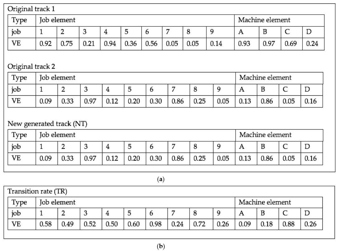
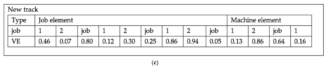
4.2.2. Track-Transition Method (TTM)

The track-transition method (TTM) is composed of three steps: (1) randomly select the original track from the pool of the tracks that were not selected by the TTM as the black box; (2) randomly generate a new track; (3) find the average value of the track for each track, denote this number as lower boundary (LB), and denote the track to which this number belongs as TLB; (4) find the minimal number of values in the tracks of the maximal value of the track that is not a member of track TLB, denote this number as the upper boundary (UB), and let the track to which the UB belongs be TUB; (5) generate transition rates (TRs) for every element of the track; (6) transit the original track to a new track by using Equation (18), while the value in track i in position h of the new track ($V{T}_{ih}^N$) is constructed. A track that is neither TLB nor TUB is called an unplaced track (UT).

$$V{T}_h^N= \left\{\begin{array}{c}V{T}_h^{TLB} if TR\le LB \\ V{T}_h^{UT} if LB<TR\le UB \\ V{T}_h^{TUB} if TR> UB \end{array}\right.$$

(18)

where $V{T}_h^{\ast }$ is the type of track, and * can be a TLB, UP, or TUB track. For example, if we have Tracks 1 and 2, and a random track as shown in Figure 1a, then the average value in the positions of Track 1, Track 2, and TR is 0.34, 0.46, and 0.51, respectively, as shown in Figure 1b. Therefore, LB = 0.34, and TLB is Track 1. The maximal numbers of VT of Track 2 and the random track are 0.83 and 0.97; therefore, UP = 0.83 and TUB = Track 2. As a result, Equation (18) was modified as shown in Equation (19), and the result of the transition is shown in Figure 1b. The result of the new track is shown in Figure 1c.

$$V{T}_h^N= \left\{\begin{array}{c}V{T}_h^1 if TR\le 0.34 \\ V{T}_h^{RT} if 0.34<TR\le 0.83 \\ V{T}_h^2 if TR>0.83 \end{array}\right.$$

(19)

After the track was generated, the decoding method shown in Section 4.1.1 was performed to find the answer for the proposed problem.

4.2.3. Multiplier Factor (MF)

MF is the neighborhood strategy of which the basic idea is to pull out the current solution from the local optimum by multiplying the current value in that position of the track by the learning multiplier factor. The new value in the track is obtained when multiplied by the multiplier using Equation (20):

$$V{T}_{ih}^{LMF}=R_{ih}V{T}_{ih}^N,$$

(20)

where $R_{ih}$ is the random number that corresponds to position h of track i, $V{T}_{ih}^{MF}$ is the track after applying the MF strategy, and $V{T}_{ih}^N$ is the track before applying the MF. An example of the MF method is shown in

Table 6. Example values of the MF method.

Type	Job Element									Machine Element
Job	1	2	3	4	5	6	7	8	9	A	B	C	D
$V{T}_{ih}^N$	0.58	0.49	0.52	0.5	0.6	0.98	0.24	0.72	0.26	0.09	0.18	0.88	0.26
$R_{ih}$	0.20	0.31	0.12	0.67	0.12	0.35	0.75	0.95	0.66	0.18	0.56	0.70	0.03
$V{T}_{ih}^{MF}$	0.12	0.15	0.06	0.33	0.07	0.34	0.18	0.68	0.17	0.02	0.10	0.62	0.01

.

After the MF operation, $V{T}_{ih}^{MF}$ uses the decoding method to obtain the solution for the proposed problem. The MF is iteratively applied to the track that selects this strategy. The predefined number of iterations was previously determined. In our method, 500 iterations were set as the stopping criterion. The MF algorithm is shown in Algorithm 6.

Algorithm 6. Multiplier factor.

Input: The value in track $({VT}_{ih}^N)$, number of jobs, number of machines   Outputs: Track after MF $(V{T}_{ih}^{MF});$   Begin i = 1   While i ≤ maximal number of iterations,   Randomly generate the random track $(R_{ih})$   Multiply ${VT}_{ih}^N$ by $R_{ih}$ and obtain $V{T}_{ih}^{MF}$   Decode $V{T}_{ih}^{MF}$ to obtain solution for the problem   i = i + 1; end while   End

Let S be the set of all feasible solutions and consider a solution Z_ijt∈ S. A neighborhood strategy associates each Z_ijt ∈ S with a neighborhood N_k (Z_ijt) ⊆ F of the solution Z_ijt. For this paper, the three neighborhood structures are SDR, TTM and MF. The time complexity of neighborhoods (N₁(Z_ijt), N₂(Z_ijt) and N₃(Z_ijt), respectively) are determined both by its respective structure and by the solution it is being applied to. The size of neighborhood N₁(Z_ijt) is O(m · n), neighborhood N₂(Z_ijt) is O(m + n) and neighborhood N₃(Z_ijt) is O(m + n).

4.3. Updating Track and Other Information

The track is updated by using Equation (21):

$$Z_{ijt+1}=Z_{ijt}+\alpha (Z_{ijt}^{pb}-Z_{ijt})+(1-\alpha )(Z_{ijt}^{gb}-Z_{ijt})+\beta (Z_{2jt}-Z_{3jt}),$$

(21)

where $Z_{ijt+1}$ is the value of track i, element j iteration t + 1. $\alpha$ and $\beta$ are predefined parameters. In this research, we defined $\alpha$ and $\beta$ as equal to 0.3. $Z_{2jt}$ is the first randomly selected track, and $Z_{3jt}$ is the second randomly selected track. We iteratively performed steps in Section 4.2; the number of iterations needed to simulate depends on the predefined parameter of number of iterations (IT).

The proposed methods were tested with the case study and randomly generated data. Results were compared with the current practice procedure. Details of the current practice procedure are below.

4.4. Current Practice Procedure

The current practice procedure (CU) in vegetable-farm case-study data assigns vegetables (jobs) to grow in all farms (machines), and it is composed of four steps, shown below.

Step 1.

Sort jobs according to energy used from least to most used, and name this list job list (JL).

Step 2.

Calculate average number of jobs per machine and call this number AM.

$$AM=\frac{Total number of jobs}{Total number of machines}$$

(22)

Step 3.

Assign jobs to machines according to JL. Job j is assigned to the machine that uses the least energy. If that machine has more jobs than AM, the next machine that uses the least energy is selected and continuously performs until all jobs are assigned.

Step 4.

Calculate the objective function of the assignment from Step 3.

4.5. Differential Evolution Algorithm

The differential evolution algorithm (DE) was used to compare it with the proposed method. DE was constructed by the following steps: (1) randomly select two other tracks that are not the track that selected DE as the black box; (2) randomly generate a new track; (3) perform the mutation process using Equation (23); (4) perform the recombination process using Equation (24); (5) perform the selection process using Equation (25) and repeat steps 1 to 5 until the termination condition is met. The DE algorithm is shown in Algorithm 7.

Algorithm 7. Differential evolution (DE) pseudocode.

Set NP, CR, F, NP (size of track) Generate initial solution Begin For G = 1 to Gmax when G = iterations and Gmax = Maximum iteration Randomly generates the set of initial solution (tracks) For N = 1 to NP Perform mutation process using $v_{i,j,G}=x_{r_4,j,G}+F\left(x_{r_2,j,G}-x_{r_3,j,G}\right)$              (23) Perform the recombination process using $u_{i,j,G}= \left\{\begin{array}{c}{v}_{i,j,G} when CR\le rand\\ x_{i,j,G} when CR>rand\end{array}\right.$                (24) Perform selection process using formula $X_{i,j,G+1}= \left\{\begin{array}{c}{U}_{i,j,G} \mathrm{if} \mathrm{f}\left(U_{i,j,G}\right) \le \mathrm{f}\left(X_{i,j,G}\right) \\ X_{i,j,G} \mathrm{otherwise} \end{array}\right.$         (25) End

5. Computational Framework and Result

The proposed metaheuristics were coded in C++ and simulated on a computer with Intel (R) Core i7-3520M CPU @ 2.90 GHz Ram 8.00 GB. We tested our algorithms on four test instances: small, medium, large, and case study. The simulation was executed five times, and the best solution among all was selected. Details of the test instances are shown in

Table 7. Test-instance details.

Group Test Instance	Number of Test Instances	Pjm (m)	Number of Jobs	Number of Machines	Ejm (THB)	TMAX	B	LMAX
Small	12	4–30	5–30	2–5	30–75	20–30%	10–50	10–100
Medium	12	4–20	40–52	3–5	30–75	20–30%	10–50	10–100
Large	12	4–20	80–134	5–8	30–75	20–30%	10–50	10–100
Case study	1	4–20	201	11	30–75	20–30%	10–50	10–100

.

Table 7 shows that we tested 37 sample data (12 small, 12 medium, and 12 large sample data, and 1 case study). For small test instances, the proposed methods were tested and compared with the optimal solution obtained from Lingo V.11 (mathematical method). For the medium and large samples, the proposed method was compared with the lower bound that was obtained by Lingo v.11 within 72 h of computation. P_jm is the processing time of job j of machine m (in minutes). E_jm is the energy used to produce job j on machine m and then converted into money units (THB). B is a constant number (THB), which is the production-overhead cost per hour of production in the factory. The proposed method was compared with the result of a traditional DE algorithm and the current practice method (CU). Details of the investigated algorithms are shown in

Table 8. Proposed-method details.

Algorithm	Detail
DE	Traditional DE
CU	Current practice procedure
VaNSAS	Variable neighborhood strategy adaptive search
SDR	Solution destroy and repair methods
TTM	Track-transition methods
MF	Multiplier factor

.

Table 8 shows that six algorithms were tested in the provided sample datasets. The performance of VaNSAS and other proposed methods was compared with that of a traditional DE.

The first experiment was executed with the small and medium test instances. The stopping criterion for Lingo was the time period when it found the optimal solution; then, it collected the best solution and computation time. The stopping criteria for all proposed methods were set as 10% of the lowest computation time of Lingo. In this case, Lingo’s lowest computation time to find the optimal solution was 651 s; thus, the stopping criteria of all proposed methods were set to 65 s. The percentage difference of all proposed methods with the obtained result from Lingo was found using Equation (26). Five replications were executed for each proposed method, and the best solution among the five runs is shown in

Table 9. Computation results of small test instances.

No	Job	m	NT	Lingo v.11		Traditional Method (THB)				Proposed Methods
				Obj. (THB)	Com. Time (sec)	DE		CU		VaNSAS		SDR		TTM		MF
						Best Sol.	Max. Error	Best Sol.	Max. Error	Best Sol.	Max. Error	Best Sol.	Max. Error	Best Sol.	Max. Error	Best Sol.	Max. Error
S-1	5	3	2	5150	872	5180	155	6782	474	5150	0	6718	268	6212	186	6237	311
S-2	6	3	2	6820	651	6954	139	7428	371	6820	0	7119	355	7023	210	6988	209
S-3	10	4	2	10,230	2056	10,230	102	13,981	699	10,230	0	12,238	367	13,148	657	13,119	655
S-4	15	3	2	10,921	1843	11,589	115	13,879	555	10,921	0	12,239	611	12,181	487	12,033	481
S-5	15	3	4	10,831	4561	10,831	108	14,713	588	10,831	0	12,815	640	12,219	366	12,172	608
S-6	20	3	3	9020	85,625	9347	280	10,895	544	9020	0	10,229	511	11,296	564	10,687	534
S-7	20	4	3	8900	80,371	9492	284	11,374	568	8900	0	11,818	472	10,722	428	10,381	415
S-8	25	4	3	11,612	76,819	12,784	255	14,981	749	11,612	0	13,209	660	13,348	533	12,987	389
S-9	25	4	2	12,360	78,371	12,788	255	14,582	583	12,360	0	13,371	401	13,794	689	12,984	649
S-10	25	4	5	11,390	67,621	11,390	113	15,378	461	11,390	0	12,879	643	12,046	602	12,288	614
S-11	28	4	5	13,705	84,004	13,794	137	17,619	880	13,705	0	14,013	560	14,237	569	14,886	744
S-12	30	4	5	11,006	89,122	12,891	257	16,716	835	11,006	0	13,310	532	14,018	420	13,873	693
% different from Lingo						4.52		29.05		0.00		14.43		15.01		13.44
% found optimal solution						25%		0%		100%		0%		0%		0%

. The statistical test is shown in

Table 10. Statistical test of small test instances.

	DE	CU	VaNSAS	SDR	TTM	MF
Lingo	0.022	0.000	0.207	0.000	0.000	0.000
DE		0.000	0.007	0.001	0.000	0.001
CU			0.000	0.000	0.001	0.001
VaNSAS				0.000	0.000	0.000
SDR					0.907	0.591
TTM						0.247

.

$$\%diff=\frac{\left(F_{opt}-F_H\right)}{F_{Opt}}\times 100\%$$

(26)

where $F_{opt}$ is the solution obtained by Lingo during the predefined computation time, and $F_H$ is the solution obtained by the proposed methods. The solutions are shown in Table 9, Table 10,

Table 11. Computation results of medium-sized test instances.

No	Job	m	NT	Exact Method	Traditional Method (THB)				Proposed Methods
				Lingo	DE		CU		VaNSAS		SDR		TTM		MF
					Best Sol.	Max. Error	Best Sol.	Max. Error	Best Sol.	Max. Error	Best Sol.	Max. Error	Best Sol.	Max. Error	Best Sol.	Max. Error
M-1	40	5	3	18,227	16,381	163	18,728	936	15,794	157	17,719	708	17,653	529	17,756	532
M-2	40	4	4	18,385	17,288	518	21,193	2119	15,992	159	17,578	703	17,233	861	17,481	874
M-3	40	4	2	19,371	16,872	337	22,371	1118	16,014	320	17,722	886	17,235	689	17,443	697
M -4	45	4	4	19,184	16,880	506	20,883	1670	16,598	497	16,957	847	17,182	687	17,084	512
M -5	45	3	2	21,827	17,998	179	21,059	1263	17,550	526	18,018	720	18,242	912	18,115	905
M -6	45	3	5	21,284	17,094	170	22,014	1761	16,881	506	17,225	689	17,188	687	17,269	518
M -7	45	5	4	21,189	16,995	339	20,913	2091	16,774	335	17,281	518	17,192	515	17,007	680
M -8	45	5	2	21,087	18,047	180	22,387	2238	17,559	351	18,817	564	19,110	764	18,349	733
M -9	50	5	4	24,871	20,122	402	25,881	2329	19,563	195	21,883	656	22,915	1145	23,120	924
M -10	50	5	3	24,483	23,287	232	24,879	2239	22,397	223	23,589	1179	23,117	924	22,996	689
M -11	50	3	5	25,598	24,448	733	26,712	2404	22,014	220	24,421	732	24,388	731	24,817	1240
M-12	52	4	6	26,515	24,481	734	26,818	1340	22,456	673	25,817	1032	25,985	1039	25,671	1026
% Improved from best objective found by Lingo					14.59		4.37		19.55		11.19		11.04		11.24

,

Table 12. Statistical test of objective function for medium-sized problem.

	DE	CU	VaNSAS	SDR	TTM	MF
Lingo	0.000	0.006	0.000	0.001	0.000	0.001
DE		0.000	0.002	0.006	0.030	0.039
CU			0.000	0.000	0.000	0.000
VaNSAS				0.000	0.001	0.001
SDR					0.777	0.962
TTM						0.767

,

Table 13. Computation results of large test instances.

No	Job	m	NT	Exact Method	Traditional Method (THB)				Proposed Methods
				Lingo	DE		CU		VaNSAS		SDR		TTM		MF
					Best Sol.	Max. Error	Best Sol.	Max. Error	Best Sol.	Max. Error	Best Sol.	Max. Error	Best Sol.	Max. Error	Best Sol.	Max. Error
L-1	80	5	6	47,968	45,871	1376	52,297	5229	39,917	1197	46,617	1864	46,521	1960	45,598	1823
L-2	80	5	5	49,351	41,278	825	45,580	4102	40,015	1200	42,893	1715	42,886	1293	42,361	1270
L-3	80	4	5	37,599	33,192	998	38,817	2329	31,108	311	34,918	1396	34,118	1847	34,287	1028
L-4	80	3	5	41,625	38,185	381	41,491	2904	36,614	366	38,811	1164	38,927	1824	38,891	1555
L-5	100	4	6	52,604	47,467	474	53,158	3721	44,581	891	48,819	2440	48,984	2275	48,816	1464
L-6	100	5	6	56,497	49,981	1499	57,619	5185	48,819	1464	50,176	1505	51,197	484	52,348	1570
L-7	100	6	6	55,823	50,187	1003	58,281	4079	47,713	954	51,810	1554	52,184	2216	52,183	1565
L-8	100	7	6	54,891	49,571	1487	55,819	3349	47,289	1418	50,972	2548	50,013	2488	51,197	2047
L-9	120	6	7	67,905	62,995	1889	68,913	6891	59,982	599	63,395	3169	64,512	1418	53,891	2155
L-10	120	7	7	67,067	63,417	1268	68,919	4135	58,813	1764	64,992	1949	63,857	4384	64,387	3219
L-11	120	8	6	65,596	60,874	608	65,817	5265	58,716	1174	59,816	1794	60,128	2678	60,016	3000
L-12	134	8	7	72,168	67,617	676	73,215	5125	64,480	644	67,764	2710	67,366	3108	67,952	2718
C-1	201	11	7	128,704	118,917	2378	129,814	11,683	110,172	2203	119,859	5992	119,347	4107	119,846	5992
% Improved from best objective found by Lingo					9.88		1.42		16.35		7.89		8.01		9.33

and

Table 14. Statistical test of objective function for large test instances.

	DE	CU	VaNSAS	SDR	TTM	MF
Lingo	0.000	0.090	0.000	0.000	0.000	0.000
DE		0.000	0.000	0.002	0.003	0.836
CU			0.000	0.000	0.000	0.000
VaNSAS				0.000	0.000	0.005
SDR					0.754	0.379
TTM						0.468

.

Computation results in Table 9, Table 10 and Table 11 show that VaNSAS performed much better than the other proposed and traditional methods did, and its performance was not significantly different from that of the exact method, while that of others significantly differed from that of the exact method. While DE, CU, SDR, TTM, and MF were different from the exact method by 4.52%, 29.05%, 14.43%, 15.01%, and 13.44%, respectively, VaNSAS was 0.00% different, which means that it could find an optimal solution for small problems 100% of the time. The maximum error is the difference between the best solution and the worst solution of each proposed algorithm. As shown in Table 9, the maximum error of VaNSAS was the lowest among others, indicating that VaNSAS had the highest solution stability.

The second experiment’s medium-sized random dataset was composed of 12 test instances. The number of jobs was randomly selected to be from 40 to 52 jobs, and the number of machines was set to be from 3 to 5. In this experiment, Lingo was executed for 48 h, and the computation time of all proposed methods was 30 min as the termination condition. After the simulation had been executed five times, the best solutions and the maximum error of medium-sized test instances were recorded in Table 11 and the statistical results are shown in Table 12.

The computation results in Table 11 and Table 12 illustrate that VaNSAS performed better than other proposed and traditional methods did. VaNSAS performed as well as the exact method did, and also showed the highest performance of solution stability over other algorithms as shown in Table 11. While others were significantly different from the exact method as seen in the statistical test result (Table 12), DE, CU, SDR, TTM, and MF were an improvement from the exact method by 14.59%, 4.37%, 11.19%, 11.04%, and 11.24%, respectively. However, VaNSAS was at 19.55%, which means that VaNSAS obtained the solution at 19.55% lower cost than that of the solution from Lingo. Lingo consumed 2880 min computation time, and VaNSAS used only 30 min.

The next experiment was tested with a large random dataset. This group of test instances was composed of 12 test instances, the number of jobs was randomly selected to be from 80 to 134, and the number of machines was set from 5 to 8 (L-1 to L-12). In this set of test instances, we included the case study, which had 201 jobs and 11 machines (C-1). In this case, Lingo was executed for 72 h to find the lower-bound solution; then, the termination condition as the computation time of all proposed heuristics was 45 min. The simulation was executed five times; the best solution and the maximum error of large instances are shown in Table 13 and the statistical results are shown in Table 14.

The computation results in Table 13 and Table 14 show that VaNSAS performed better than other proposed and traditional methods did. The performance of VaNSAS is similar to the exact method, while others were significantly different from the exact methods. DE, CU, SDR, TTM, and MF were 9.88%, 1.42%, 7.89%, 8.01%, and 9.33%, respectively, different from the exact method. In addition, VaNSAS was 16.35% different from the exact method, which means it could find 16.35% lower cost than how much Lingo could. The maximum error of each method indicates that VaNSAS outperformed other methods in terms of solution stability. In addition, Lingo required 2880 min of computation time while VaNSAS only required 45 min.

6. Conclusions and Outlook

Green machine-scheduling problems, such as optimization problem related to energy concerns, are paid more attention by a wide array of industries, since environmental awareness is part of industrial manufacturing sustainability. This paper presents a novel method called variable neighborhood strategy adaptive search (VaNSAS) to solve the parallel-machine-scheduling problem in order to minimize energy consumption while considering job priority and makespan control. Although VaNSAS successfully improved solution-search performance in previous studies [17,22,36,37,38], none had accounted for energy consumption, late delivery charge, and production overhead. The advantage of applying VaNSAS in this study was that its algorithms search for the best possible solution in many different areas by using several searching approaches, thereby moving to find more diversification and intensification at all times depending on the designed black-box methods. In addition, we improved the solution-search performance of VaNSAS by presenting new neighborhood search strategies: (1) solution destroy and repair (SDR); (2) track-transition method (TTM); and (3) multiplier factor (MF). The proposed methods were performed in three sets of test instances and one case study, and compared with the exact method.

Computation results show that the proposed VaNSAS outperformed all traditional and other proposed methods. It performed as well as the exact method did, illustrated in the small problem, while the traditional DE could find only 25%; CU, SDR, TTM, and MF could not find the optimal solution at all, while VaNSAS could find 100% of the optimal solution. Even by increasing the problem size, VaNSAS still gave promising results, as it could improve the solution quality by 16.35–19.55% of the solution obtained from the exact method with 30–45 min of computation time, while the exact method required 48–72 h. In the medium-sized and large samples, DE, SDR, TTM, and MF could also improve the solution quality by 7.89–14.59% more than the exact method. In addition, the current practice gave a worse solution than that of the exact method, including all proposed methods, by 1.42–4.37%.

The excellent solution-search efficiency of VaNSAS in this study and its advantage of a flexible neighborhood search scheme allow researchers to further develop and design new mechanisms for improving solution quality. Additionally, it would be interesting to implement the proposed VaNSAS in various problem areas, such as production planning in a real manufacturing environment, while considering other additional factors or constraints, e.g., the study of the capability of each type of machine, job restriction, and customer-order scheduling.

References

1. EIA. Available online: https://www.eia.gov/outlooks/aeo/data/browser/#/?id=37-AEO2020&cases=ref2020&sourcekey=1 (accessed on 28 March 2021).
2. EIA. Available online: https://www.eia.gov/outlooks/aeo/data/browser/#/?id=22-AEO2020&cases=ref2020&sourcekey=0 (accessed on 28 March 2021).
3. Fang, K.T.; Lin, B.M. Parallel-machine scheduling to minimize tardiness penalty and power cost. Comput. Ind. Eng. 2013, 64, 224–234. [Google Scholar] [CrossRef]
4. Che, A.; Zhang, S.; Wu, X. Energy-conscious unrelated parallel machine scheduling under time-of-use electricity tariffs. J. Clean. Prod. 2017, 156, 688–697. [Google Scholar] [CrossRef]
5. Abikarram, J.B.; McConky, K.; Proano, R. Energy Cost Minimization for Unrelated Parallel Machine Scheduling under Real Time and Demand Charge Pricing. J. Clean. Prod. 2019, 208, 232–242. [Google Scholar] [CrossRef]
6. Cui, W.; Lu, B. A Bi-Objective Approach to Minimize Makespan and Energy Consumption in Flow Shops with Peak Demand Constraint. Sustainability 2020, 12, 4110. [Google Scholar] [CrossRef]
7. Fang, K.; Uhan, N.; Zhao, F.; Sutherland, J.W. A New Approach to Scheduling in Manufacturing for Power Consumption and Carbon Footprint Reduction. J. Manuf. Syst. 2011, 30, 234–240. [Google Scholar] [CrossRef]
8. Yin, L.; Li, X.; Lu, C.; Gao, L. Energy-Efficient Scheduling Problem Using an Effective Hybrid Multi-Objective Evolutionary Algorithm. Sustainability 2016, 8, 1268. [Google Scholar] [CrossRef] [Green Version]
9. Mansouri, S.A.; Aktas, E.; Besikci, U. Green Scheduling of a Two-Machine Flowshop: Trade-off between Makespan and Energy Consumption. Eur. J. Oper. Res. 2016, 248, 772–788. [Google Scholar] [CrossRef] [Green Version]
10. Liu, C.-H.; Huang, D.-H. Reduction of Power Consumption and Carbon Footprints by Applying Multi-Objective Optimisation via Genetic Algorithms. Int. J. Prod. Res. 2013, 52, 337–352. [Google Scholar] [CrossRef]
11. Zhang, Z.; Wu, L.; Peng, T.; Jia, S. An Improved Scheduling Approach for Minimizing Total Energy Consumption and Makespan in a Flexible Job Shop Environment. Sustainability 2019, 11, 179. [Google Scholar] [CrossRef] [Green Version]
12. Fysikopoulos, A.; Pastras, G.; Alexopoulos, T.; Chryssolouris, G. On a Generalized Approach to Manufacturing Energy Efficiency. Int. J. Adv. Manuf. Technol. 2014, 73, 1437–1452. [Google Scholar] [CrossRef] [Green Version]
13. Zeng, Z.; Chen, X.; Wang, K. Energy Saving for Tissue Paper Mills by Energy-Efficiency Scheduling under Time-of-Use Electricity Tariffs. Processes 2021, 9, 274. [Google Scholar] [CrossRef]
14. Liu, C.-H.; Nanthapodej, R.; Hsu, S.-Y. Scheduling Two Interfering Job Sets on Parallel Machines under Peak Power Constraint. Prod. Eng. 2018, 12, 611–619. [Google Scholar] [CrossRef]
15. Lin, D.-Y.; Huang, T.-Y. A Hybrid Metaheuristic for the Unrelated Parallel Machine Scheduling Problem. Mathematics 2021, 9, 768. [Google Scholar] [CrossRef]
16. Vakhania, N.; Werner, F. Branch Less, Cut More and Schedule Jobs with Release and Delivery Times on Uniform Machines. Mathematics 2021, 9, 633. [Google Scholar] [CrossRef]
17. Kusoncum, C.; Sethanan, K.; Pitakaso, R.; Hartl, R.F. Heuristics with Novel Approaches for Cyclical Multiple Parallel Machine Scheduling in Sugarcane Unloading Systems. Int. J. Prod. Res. 2020, 1–19. [Google Scholar] [CrossRef]
18. Lin, Y.K.; Pfund, M.E.; Fowler, J.W. Heuristics for Minimizing Regular Performance Measures in Unrelated Parallel Machine Scheduling Problems. Comput. Oper. Res. 2011, 38, 901–916. [Google Scholar] [CrossRef]
19. Zhou, S.; Li, X.; Du, N.; Pang, Y.; Chen, H. A Multi-Objective Differential Evolution Algorithm for Parallel Batch Processing Machine Scheduling Considering Electricity Consumption Cost. Comput. Oper. Res. 2018, 96, 55–68. [Google Scholar] [CrossRef]
20. Sethanan, K.; Jamrus, T. Hybrid Differential Evolution Algorithm and Genetic Operator for Multi-Trip Vehicle Routing Problem with Backhauls and Heterogeneous Fleet in the Beverage Logistics Industry. Comput. Ind. Eng. 2020, 146, 106571. [Google Scholar] [CrossRef]
21. Theeraviriya, C.; Sirirak, W.; Praseeratasang, N. Location and Routing Planning Considering Electric Vehicles with Restricted Distance in Agriculture. World Electr. Veh. J. 2020, 11, 61. [Google Scholar] [CrossRef]
22. Jirasirilerd, G.; Pitakaso, R.; Sethanan, K.; Kaewman, S.; Sirirak, W.; Kosacka-Olejnik, M. Simple Assembly Line Balancing Problem Type 2 by Variable Neighborhood Strategy Adaptive Search: A Case Study Garment Industry. J. Open Innov. Technol. Mark. Complex. 2020, 6, 21. [Google Scholar] [CrossRef] [Green Version]
23. Zeng, Y.; Che, A.; Wu, X. Bi-Objective Scheduling on Uniform Parallel Machines Considering Electricity Cost. Eng. Optim. 2017, 50, 19–36. [Google Scholar] [CrossRef]
24. Sethanan, K.; Wisittipanich, W.; Wisittipanit, N.; Nitisiri, K.; Moonsri, K. Integrating Scheduling with Optimal Sublot for Parallel Machine with Job Splitting and Dependent Setup Times. Comput. Ind. Eng. 2019, 137, 106095. [Google Scholar] [CrossRef]
25. Li, K.; Zhang, X.; Leung, J.Y.-T.; Yang, S.-L. Parallel Machine Scheduling Problems in Green Manufacturing Industry. J. Manuf. Syst. 2016, 38, 98–106. [Google Scholar] [CrossRef]
26. Al-Shayea, A.M.; Saleh, M.; Alatefi, M.; Ghaleb, M. Scheduling Two Identical Parallel Machines Subjected to Release Times, Delivery Times and Unavailability Constraints. Processes 2020, 8, 1025. [Google Scholar] [CrossRef]
27. Eltaeib, T.; Mahmood, A. Differential Evolution: A Survey and Analysis. Appl. Sci. 2018, 8, 1945. [Google Scholar] [CrossRef] [Green Version]
28. Storn, R.; Price, K. Differential Evolution—A Simple and Efficient Heuristic for Global Optimization over Continuous Spaces. J. Glob. Optim. 1997, 11, 341–359. [Google Scholar] [CrossRef]
29. Wang, W.-L.; Wang, H.-Y.; Zhao, Y.-W.; Zhang, L.-P.; Xu, X.-L. Parallel Machine Scheduling with Splitting Jobs by a Hybrid Differential Evolution Algorithm. Comput. Oper. Res. 2013, 40, 1196–1206. [Google Scholar] [CrossRef]
30. Praseeratasang, N.; Pitakaso, R.; Sethanan, K.; Kosacka-Olejnik, M.; Theeraviriya, C. Adaptive Large Neighborhood Search to Solve Multi-Level Scheduling and Assignment Problems in Broiler Farms. J. Open Innov. Technol. Mark. Complex. 2019, 5, 37. [Google Scholar] [CrossRef] [Green Version]
31. Praseeratasang, N.; Pitakaso, R.; Sethanan, K.; Kaewman, S.; Golinska-Dawson, P. Adaptive Large Neighborhood Search for a Production Planning Problem Arising in Pig Farming. J. Open Innov. Technol. Mark. Complex. 2019, 5, 26. [Google Scholar] [CrossRef] [Green Version]
32. Pitakaso, R.; Sethanan, K. Adaptive Large Neighborhood Search for Scheduling Sugarcane Inbound Logistics Equipment and Machinery under a Sharing Infield Resource System. Comput. Electron. Agric. 2019, 158, 313–325. [Google Scholar] [CrossRef]
33. Cota, L.P.; Guimarães, F.G.; de Oliveira, F.B.; Souza, M.J.F. An Adaptive Large Neighborhood Search with Learning Automata for the Unrelated Parallel Machine Scheduling Problem. Available online: https://0-ieeexplore-ieee-org.brum.beds.ac.uk/abstract/document/7969312 (accessed on 26 February 2021).
34. Khamsing, N.; Chindaprasert, K.; Pitakaso, R.; Sirirak, W.; Theeraviriya, C. Modified ALNS Algorithm for a Processing Application of Family Tourist Route Planning: A Case Study of Buriram in Thailand. Computation 2021, 9, 23. [Google Scholar] [CrossRef]
35. Cota, L.P.; Guimarães, F.G.; Ribeiro, R.G.; Meneghini, I.R.; de Oliveira, F.B.; Souza, M.J.F.; Siarry, P. An Adaptive Multi-Objective Algorithm Based on Decomposition and Large Neighborhood Search for a Green Machine Scheduling Problem. Swarm Evol. Comput. 2019, 51, 100601. [Google Scholar] [CrossRef]
36. Theeraviriya, C.; Pitakaso, R.; Sethanan, K.; Kaewman, S.; Kosacka-Olejnik, M. A New Optimization Technique for the Location and Routing Management in Agricultural Logistics. J. Open Innov. Technol. Mark. Complex. 2020, 6, 11. [Google Scholar] [CrossRef] [Green Version]
37. Pitakaso, R.; Sethanan, K.; Theeraviriya, C. Variable Neighborhood Strategy Adaptive Search for Solving Green 2-Echelon Location Routing Problem. Comput. Electron. Agric. 2020, 173, 105406. [Google Scholar] [CrossRef]
38. Pitakaso, R.; Sethanan, K.; Jirasirilerd, G.; Golinska-Dawson, P. A Novel Variable Neighborhood Strategy Adaptive Search for SALBP-2 Problem with a Limit on the Number of Machine’s Types. Ann. Oper. Res. 2021. [Google Scholar] [CrossRef]
39. Liu, C.-H. Approximate Trade-off between Minimisation of Total Weighted Tardiness and Minimisation of Carbon Dioxide (CO2) Emissions in Bi-Criteria Batch Scheduling Problem. Int. J. Comput. Integr. Manuf. 2013, 27, 759–771. [Google Scholar] [CrossRef]
40. Pan, Z.; Lei, D.; Zhang, Q. A New Imperialist Competitive Algorithm for Multiobjective Low Carbon Parallel Machines Scheduling. Math. Probl. Eng. 2018, 2018, 1–13. [Google Scholar] [CrossRef] [Green Version]
41. Chen, B.; Potts, C.N.; Woeginger, G.J. A Review of Machine Scheduling: Complexity, Algorithms and Approximability. Handb. Comb. Optim. 1998, 1493–1641. [Google Scholar] [CrossRef]
42. Pinedo, M.L. Scheduling; Springer International Publishing: Cham, Swizerland, 2016. [Google Scholar] [CrossRef]
43. Behera, D.K. Complexity on Parallel Machine Scheduling: A Review. Lect. Notes Mech. Eng. 2012, 373–381. [Google Scholar] [CrossRef]
44. Theeraviriya, C.; Ruamboon, K.; Praseeratasang, N. Solving the Multi-Level Location Routing Problem Considering the Environmental Impact Using a Hybrid Metaheuristic. Int. J. Eng. Bus. Manag. 2021, 13, 184797902110173. [Google Scholar] [CrossRef]
45. Mouzon, G.; Yildirim, M.B.; Twomey, J. Operational Methods for Minimization of Energy Consumption of Manufacturing Equipment. Int. J. Prod. Res. 2007, 45, 4247–4271. [Google Scholar] [CrossRef] [Green Version]
46. Angel, E.; Bampis, E.; Kacem, F. Energy Aware Scheduling for Unrelated Parallel Machines. Available online: https://0-ieeexplore-ieee-org.brum.beds.ac.uk/abstract/document/6468361 (accessed on 27 February 2021).
47. Sobottka, T.; Kamhuber, F.; Heinzl, B. Simulation-Based Multi-Criteria Optimization of Parallel Heat Treatment Furnaces at a Casting Manufacturer. J. Manuf. Mater. Process. 2020, 4, 94. [Google Scholar] [CrossRef]
48. Nanthapodej, R.; Liu, C.-H.; Nitisiri, K.; Pattanapairoj, S. Hybrid Differential Evolution Algorithm and Adaptive Large Neighborhood Search to Solve Parallel Machine Scheduling to Minimize Energy Consumption in Consideration of Machine-Load Balance Problems. Sustainability 2021, 13, 5470. [Google Scholar] [CrossRef]
49. Chaudhry, I.A.; Elbadawi, I.A. Minimisation of total tardiness for identical parallel machine scheduling using genetic algorithm. Sādhanā 2017, 42, 11–21. [Google Scholar] [CrossRef] [Green Version]
50. Pei, J.; Cheng, B.; Liu, X.; Pardalos, P.M.; Kong, M. Single-Machine and Parallel-Machine Serial-Batching Scheduling Problems with Position-Based Learning Effect and Linear Setup Time. Ann. Oper. Res. 2017, 272, 217–241. [Google Scholar] [CrossRef]
51. Maecker, S.; Shen, L. Solving Parallel Machine Problems with Delivery Times and Tardiness Objectives. Ann. Oper. Res. 2019, 285, 315–334. [Google Scholar] [CrossRef]
52. Zhou, S.; Liu, M.; Chen, H.; Li, X. An Effective Discrete Differential Evolution Algorithm for Scheduling Uniform Parallel Batch Processing Machines with Non-Identical Capacities and Arbitrary Job Sizes. Int. J. Prod. Econ. 2016, 179, 1–11. [Google Scholar] [CrossRef]
53. Wu, X.; Che, A. A Memetic Differential Evolution Algorithm for Energy-Efficient Parallel Machine Scheduling. Omega 2019, 82, 155–165. [Google Scholar] [CrossRef]
54. Li, D.; Wang, J.; Qiang, R.; Chiong, R. A Hybrid Differential Evolution Algorithm for Parallel Machine Scheduling of Lace Dyeing Considering Colour Families, Sequence-Dependent Setup and Machine Eligibility. Int. J. Prod. Res. 2020, 1–17. [Google Scholar] [CrossRef]
Figure 1. Example of the track-transition method (TTM) procedure: (a) Tracks 1 and 2, and new random track; (b) Transition rate (TR); (c) Result of new transition.
Applsci 11 05311 g001aApplsci 11 05311 g001b