
Quality-Aware Resource Model Discovery


1
School of Information Convergence, Kwangwoon University, Seoul 01897, Korea
2
Department of Industrial and Management Engineering, Pohang University of Science and Technology, Pohang 37673, Korea
3
Department of Computer Science, RWTH Aachen University, 52074 Aachen, Germany
4
Mechatronics Research and Development Center, Samsung Electronics Company Ltd., Hwaseong 18448, Korea
*
Author to whom correspondence should be addressed.
Appl. Sci. 2021, 11(12), 5730; https://0-doi-org.brum.beds.ac.uk/10.3390/app11125730
Submission received: 17 May 2021
/
Revised: 10 June 2021
/
Accepted: 17 June 2021
/
Published: 21 June 2021
(This article belongs to the Special Issue Big Data and AI for Process Innovation in the Industry 4.0 Era)
Abstract
:Context-aware process mining aims at extending a contemporary approach with process contexts for realistic process modeling. Regarding this discipline, there have been several attempts to combine process discovery and predictive process modeling and context information, e.g., time and cost. The focus of this paper is to develop a new method for deriving a quality-aware resource model. It first generates a resource-oriented transition system and identifies the quality-based superior and inferior cases. The quality-aware resource model is constructed by integrating these two results, and we also propose a model simplification method based on statistical analyses for better resource model visualization. This paper includes tooling support for our method, and one of the case studies on a semiconductor manufacturing process is presented to validate the usefulness of the proposed approach. We expect our work is practically applicable to a range of fields, including manufacturing and healthcare systems.
1. Introduction
Process mining is a promising discipline generating process-related knowledge from event logs obtained from enterprise systems [1]. It aims to discover, monitor, and improve business processes with numerous techniques, including process discovery, conformance checking, and process enhancement [1]. Due to the advantages of process mining, i.e., the help in clearly understanding and deriving insights of processes, it has been applied to different industries, such as healthcare and manufacturing, and contributed to the digital transformation [2].
While process mining mainly focuses on the control-flow perspective, some approaches endeavor to incorporate other perspectives such as time, cost, and quality perspectives to represent process contexts, enabling context-aware process mining. In [3], an approach for context-aware inductive process discovery is suggested, which combines the control-flow and context information under a single roof. In addition, contextual data are utilized to increase the accuracy of the prediction of process performance indicators, e.g., remaining time [4]. In [5], the author presents a generic framework for deploying context-aware performance analysis in a business process.
In many domains such as manufacturing, healthcare, and service, performances of processes are often highly related to the resources, i.e., process participants [6]. For instance, in manufacturing, the machines involved in the production have huge influences on the quality of final products [7]. Moreover, in healthcare, each medical staff member has a different level of proficiency, resulting in differences in patient satisfaction [8]. In this regard, there have been attempts to analyze resources using process mining techniques for quality management [9]. For instance, [10] analyzes the relationship between individual resources and quality. However, the approach for connecting the quality to resource paths, networks, or models was insufficient.
In this work, we propose a method to discover quality-aware resource models. The resource model explains which resource paths result in high-quality cases (e.g., complete products in manufacturing and high satisfaction of patients in healthcare). The proposed method takes an event log as input and subsequently produces a simplified resource model, annotating the quality data. In more detail, it has five steps, including resource model generation, superior and inferior case identification, integrated model construction, statistical analysis on resources, and model simplification. In addition, to sufficiently perform these steps, we employ case-annotated transition systems and multiple statistical analysis techniques.
The main contribution of this paper is as follows:
- Introducing a quality-aware resource model mining algorithm, which integrates the resource-oriented transition system and quality-based superior and inferior cases (Section 3.2, Section 3.3 and Section 3.4);
- Suggesting a model simplification method based on statistical analyses (Section 3.5 and Section 3.6);
- Providing tooling support for the proposed approach (Section 4).
In addition, to show the usefulness of the proposed methodology, we provide one of the case studies on a semiconductor manufacturing process at a manufacturing company in Korea.
The remainder of this paper is organized as follows. The next session discusses related works, and Section 3 explains the proposed methodology. Section 4 discusses the tool implemented in this research. Section 5 presents the application in the case study, and Section 6 concludes with the summary, limitations, and future works.
2. Related Works
In the process mining discipline, automated process discovery in terms of the control-flow perspective has been a principal research stream for the last two decades [11]. Beyond the control-flow perspective, prior works using data attributes, i.e., process contexts, have received considerable interest to improve and complement the processes [3,4,5,12,13,14,15,16,17,18]. In other words, context-aware process mining approaches have covered a range of research themes, including process discovery, conformance checking, and enhancement [3,4,5,12,13,14,15,16,17,18].
Most context-aware process discovery efforts have followed a two-step approach: producing a process model with the control-flow and then annotating context data, e.g., time, cost, and decisions, on the model [12,13,14]. For example, time-related contexts, e.g., service time, bottlenecks, and utilization, were annotated on the transition systems, and this research enabled the prediction of time-related values [12]. In addition, Tu and Song employed cost-related contexts in manufacturing processes, including labor costs, material costs, and overhead costs [13]. Rozinat and van der Aalst identified the influence of case and event attributes on the choices, i.e., XOR-split, in the processes [14]. In more detail, they uncovered the rules explaining the choices based on the characteristics of cases, and those were annotated in the process model. In addition to these prior works, i.e., “control-flow first” approaches, there was an attempt to produce a context-aware inductive process model, which considers the control-flow and context information at the same time [3]. The authors constructed the process tree with data semantics instead of control-flow semantics.
Regarding conformance checking, there have been attempts to compare process models and event logs in terms of both control-flow and other process contexts [15,16,17]. Mannhardt et al. [15] proposed a method that considers data dependencies, resource assignments, and time constraints for conformance checking. In addition, the authors suggested a customizable cost function to balance the deviations from multiple perspectives. Conformance checking with process contexts has been actively utilized in declarative process models [16,17]. In general, declarative process models should have numerous process constraints to accomplish business goals; most process constraints are defined in multi-perspectives, and conformance checking is utilized to evaluate them.
Contextual information has also been utilized for process enhancement [4,5,18]. For example, a generic framework for operating context-aware performance analysis was presented to analyze performance characteristics from multiple perspectives [5]. In addition, the authors showed that the accuracy of the prediction of process performance indicators, including remaining time, can be improved using contextual data [4]. There was also an approach to utilize process contexts to receive more homogeneous data from trace clustering [18].
There have been multiple attempts on context-aware process mining to discover realistic processes and improve them. As mentioned in Section 1, however, there was a lack of connecting resource network models to process contexts. In particular, although the quality is a necessary measure as one of the Devil’s quadrangles, it has not been a crucial element in contextual data. As such, our work resolves these limitations and presents a quality-aware resource model discovery method.
3. Quality-Aware Resource Model Discovery
This section describes our approach to derive a quality-aware resource model. In this regard, Section 3.1 introduces the overview of the proposed approach in this paper, and Section 3.2, Section 3.3, Section 3.4, Section 3.5 and Section 3.6 gives detailed explanations for individual steps in the methodology.
3.1. Overview
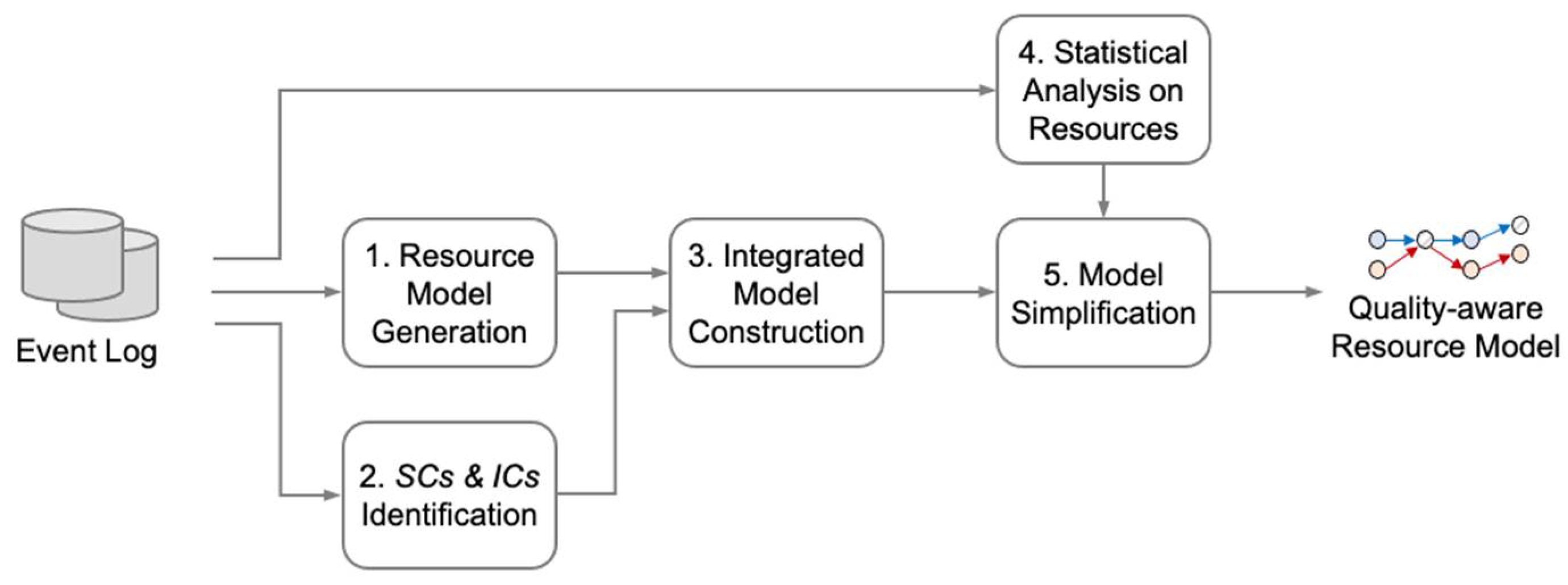
This section presents the whole structure of the proposed methodology, i.e., quality-aware resource model discovery, as depicted in Figure 1. Our approach includes five steps: model generation, superior and inferior case identification, integrated model construction, statistical analysis on resources, and model simplification. It first takes an event log as input and produces a resource-oriented transition system representing the resource behaviors described in the log. Second, based on quality data, we identify the cases recorded as relatively superior or inferior to others. Afterwards, the extracted resource model and the identified superior and inferior cases are combined into a quality-aware resource model that distinguishes the high- and low-quality-generating resource paths. The discovered model, however, may be remarkably complicated since plenty of resources are generally engaged in a business process. Thus, the fourth step performs a series of statistical analyses on the performance of resources to determine resources that have high impacts on the quality. Lastly, we simplify the discovered model using the results of the statistical analysis.
Before presenting how to implement the quality-aware resource model, we define an event log in Section 3.1.1.
3.1.1. Event Logs
We utilize a common model of event logs, a collection of process instances, i.e., cases [1]. Every case has a specific trace composed of a series of multiple events, and events can have several attributes, including activities, originators, and timestamps. In addition, the log contains the quality of cases, e.g., yield in production systems, death rates or length of stays in healthcare systems, as a required attribute. It serves as context information for a process. Note that this approach focuses on the quality of business processes, but we can consider other attributes, such as costs or overall time spent on process instances. In that case, we should collect these attributes in the event log. The corresponding formalization is defined in Definition 1.
Definition 1.
(Event, Attribute, Case, Quality, Event log). Let E be the event universe. Events may have several attributes (e.g., activity, originator, timestamp). Let AN be a set of attribute names. For any event and any attribute name is the value of the attribute an for event e. If event e does not have an attribute value, = (null value). Let be the set of cases. For any case and any attribute name : is the value of the attribute an for case c. If case c does not have an attribute value, = (null value). Each case has mandatory attributes, i.e., trace (t) and quality (q): and .An event log L is a collection of possible cases.
Table 1 describes a fragment of the synthetic event log, including context information, i.e., quality. As presented in Definition 1, each case includes several events that have additional information, including activities, originators, and timestamps. For example, CaseID C1 has four different events, and the first event is relevant to Activity A that was performed by Originator M1 and completed at 10:30 on 1 January 2021. In addition, the same quality value, 0.95 is recorded in all events of CaseID C1 as a case attribute.
3.2. Resource Model Generation
The initial step of the proposed approach is to produce a model representing resource behaviors in a log, i.e., discovery in process mining [1]. In the business process discipline, there are numerous process modeling notations such as Petri-nets [19], YAWL (Yet Another Workflow Language) [20], and BPMN (Business Process Modeling Notation) [21]. This paper employs transition systems [12], the most basic and uncomplicated process modeling notation. Transition systems are frequently utilized in the process mining discipline, and it has the advantage of deriving meaningful results that summarize the behaviors in the log, based on various abstraction techniques [12].
Section 3.2.1 explains how to derive a transition system from the event log, and Section 3.2.2 introduces a context-aware transition system.
3.2.1. Transition Systems
Transition systems are composed of states, events, and transitions, and they can be produced from event logs through a series of steps [12]. States represent the status where an event in a process is performed, while transitions refer to the relationship that changes a state as an event is performed in a particular state. In addition, a transition system has one or more initial states and final states. In a nutshell, a transition system is built by connecting a chain of transitions from initial states to final states. Definition 2 describes the formal definition of building transition systems from event logs.
Definition 2.
(State representation function, Event representation function, Transition system). Let L be an event log. Let and be a set of possible traces and events. A state representation function is a function that maps traces to state representations, where is the set of possible state representations. An event representation function is a function that maps events to event representations, where is the set of possible event representations. A transition system TS is defined as a triplet (S, E, T), where , , and with is the set of states, the set of events, and the set of transitions.
Transition systems can be produced in different forms from the same event log L based on event and state representation functions. First, the event representation function repe(e) is associated with what types (i.e., event attributes) of transition systems are derived. If we want to build a transition system relevant to the activity, the event representation function should be established such that . Alternatively, if interested in the originator, it is necessary to determine the event representation function such that . We can also apply both the activity and the originator at the same time such that . As far as states are concerned, the state representation function reps() is utilized with different types of abstractions, where is a trace. In addition, we can consider the horizon, which means how many events are included from the prefix to determine the states with . Here, signifies to the head of the sequence with the first k elements from the trace
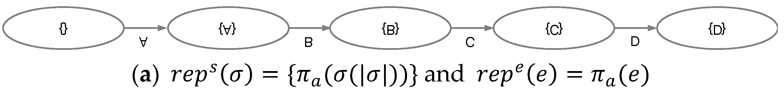
Figure 2 presents examples of transition systems derived from the same event log in Table 1. Figure 2a is the activity-oriented transition system where only the last event is utilized, and the event and the state representation functions are applied such that and . Contrary to this, Figure 2b,c are the resource-oriented transition systems. Two transitions systems, however, are separated with the horizon value. Similar to Figure 2a,b includes only the last event, i.e., , whereas Figure 2c uses the complete sequence, i.e., and the combination of the activity and the resource, i.e., . Note that this paper covers the transition systems that uses both the activity and the originator.
3.2.2. Case-Annotated Transition Systems
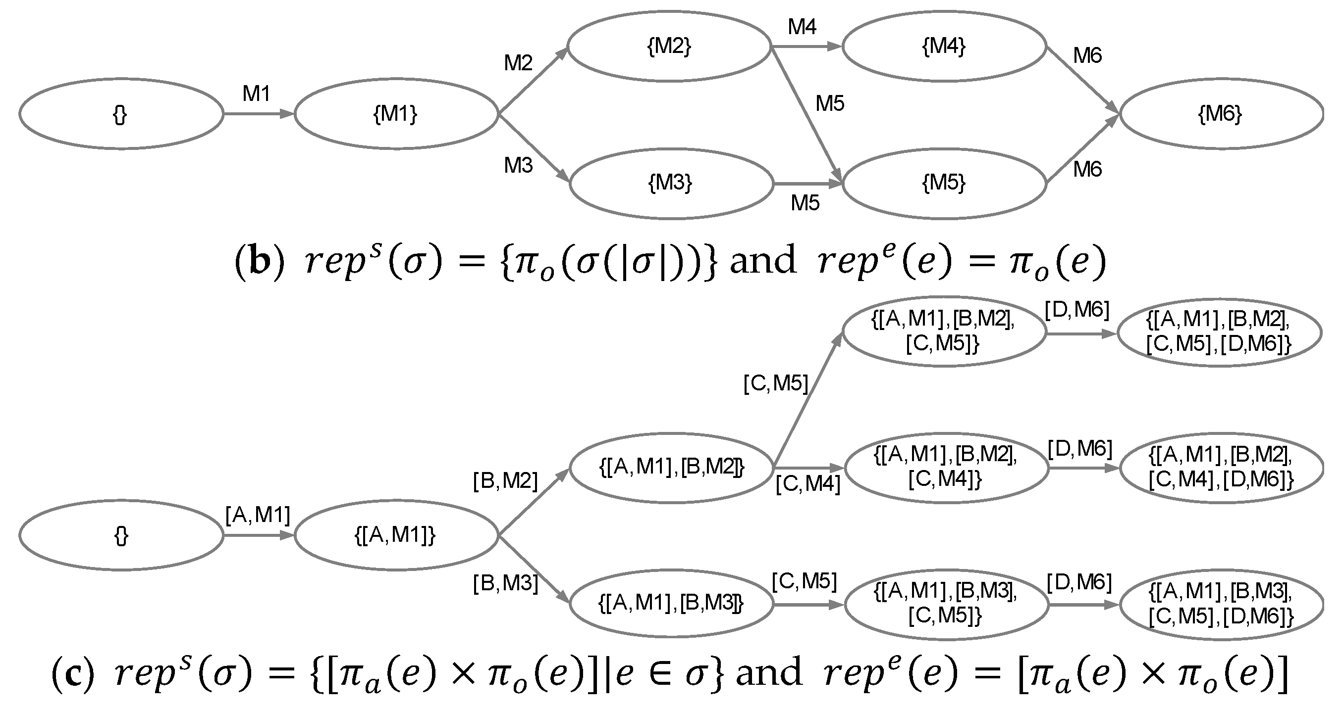
Case-annotated transition systems are generated by annotating the cases recorded in event logs into transition systems. Definition 3 gives the formal explanation for annotating the cases into transition systems and deriving the case-annotated transition systems CTS = (S, E, T, As, Ae). The state and event annotation functions and adds the cases into states and events, respectively. Figure 3 gives an example of transition systems that annotate cases based on the event log in Table 1 and the process model in Figure 2b. Figure 3 provides a case-annotated transition system (S, E, T, As, Ae) with and . For example, the annotated cases on the state M1, i.e., , are [C1, C2, C3], while the cases of the arc between the state M1 and M2, i.e., , are [C1, C3].
Definition 3.
(Case-annotated transition system)Let L be an event log, and TS = (S, E, T) be a transition system based on a state representation function and an event representation function . The annotation functions and where for any state and any event :
A case-annotated transition system CTS is defined such that ().
3.3. Superior and Inferior Case Identification
In this section, we give a detailed explanation of how to identify the superior cases, i.e., SCs, and the inferior cases, i.e., ICs, based on the quality values. To this end, it is necessary to employ a couple of statistical functions. First, we verify the normality of the empirical distribution for quality values from the event logs. In accordance with the result, the corresponding step to obtain SCs and ICs is separated. As a method to test the normality, we employ the Kolmogorov–Smirnov one sample test [22], i.e., KS1S. It investigates whether the empirical quality distribution from the log and the normal distribution are statistically the same or not. The test statistic D is , where is the empirical cumulative distribution and is the cumulative normal distribution. The null (H0) and the alternative (H1) hypothesis are established such that and , respectively. If normality is satisfied, QCs and ICs are determined based on the mean () and the standard deviation () of the quality distribution. Conversely, when the normality condition is unsatisfactory, the median () and the median absolute deviation () [23] values are utilized. Based on the calculated mean/median and the standard deviation/MAD, we can create a certain range that represents just a mediocre quality, i.e., where w is a user-specified weight. After that, the quality values of all cases are evaluated whether they are within or outside the range. If the quality values are higher than the maximum value of the range, the corresponding cases are classified as SCs. On the other hand, if cases have a lower quality than the minimum value of the range, they belong to ICs.
Algorithm 1 explains the proposed approach to identify the superior and inferior cases in detail.
| Algorithm 1.IdentifyingSIcases(L, w) |
| Input An event log L A weight to specify mediocre range of quality w Output A set of cases that have relatively high quality (i.e., the superior cases) S A set of cases that have relatively low quality (i.e., the inferior cases) I Let C be the set of cases in an event log L and be the quality value for a case . KS1S is the function to conduct the Kolmogorov–Smirnov one sample test for identifying whether a sample follows the normal distribution or not. Average, Stddev, and Median are functions to calculate average, standard deviation, and median values of a specific distribution, respectively. normality_result KS1S(Q) S , I if normality_result is True then Average(Q) Stddev(Q) S I else Median(Q) b 1/q(0.75) (where, q(0.75) is the 0.75 quantile of the distribution) Median() S I return S, I |
3.4. Integrated Model Construction
In the last two sections, we explained how to produce case-annotated transition systems and identify the superior and inferior cases based on event logs. The following phase integrates the results from the last two steps. In other words, quality-based superior and inferior paths are established on the discovered resource model. First, we calculate SCs ratio (SCR) and ICs ratio (ICR) for each state and event, showing how many superior cases or inferior cases are included among all the instances, respectively. These two values become the materials to evaluate the performance of states and events. Formally, SCR and ICR are defined as follows.
Definition 4.
(SCs ratio, ICs ratio)Let L be an event log, and CTS = () be a case-annotated transition system based on the log L. Let S, I be the set of the superior and the inferior cases, respectively. SCs ratio for states SCRs and events SCRe and ICs ratio for states ICRs and events ICRe are defined as follows.
The performance of states and events is assessed using two measurements: Between sum (i.e., BWS) and Between difference (i.e., BWD). BWS is calculated by summing up both SCs ratio and ICs ratio for a specific state or an event. It refers to the paramountcy of the state or the event itself. After that, BWD is employed to identify whether a particular state or an event belongs to the superior paths or the inferior paths. If BWD is greater than 0, i.e., SCR > ICR, the relevant state or event is determined as the part of the superior paths that lead to a high quality. In the opposite case, i.e., SCR < ICR, it is considered as a piece of the inferior paths. Based on the case-annotated transition system, an integrated model is constructed by incorporating BWS and BWD, such that IM = (CTS, BWS, BWD). These are defined as follows.
Definition 5.
(BW sum, BW difference, Integrated model) Let SCRs and SCRe the superior case ratio for states and events, respectively. Let ICRs and ICRe the inferior case ratio for states and events, respectively. BW sum for states BWSs and events BWSe and BW difference for states BWDs and events BWDe are defined as follows.
−BWSs = BCRs + WCRs
−BWSe = BCRe + WCRe
−BWDs = BCRs − WCRs
−BWDe = BCRe − WCRe
−BWSe = BCRe + WCRe
−BWDs = BCRs − WCRs
−BWDe = BCRe − WCRe
Let BWS and BWD be the set of BW sum and BW difference, respectively. Then, an integrated model IM = (CTS, BWS, BWD) is the case-annotated transition system including BWS and BWD.
Note that BWS and BWD values are utilized to visualize the derived model’s border and arcs. By comparing BWS and BWD with user-defined thresholds, the superior and the inferior paths can be painted differently. As a result, users can quickly recognize the meaningful paths in the model. Details are provided in Section 4.2.
3.5. Statistical Analysis on Resources
As discussed in Section 1, the discovered integrated quality-aware resource model has a limitation in that it has a high complexity as the process gets more extended or more resources are engaged in activities. To overcome this limitation, we need to find out mainline states and transitions that have a statistical significance to quality and simplify it. This section suggests a series of procedures by exploiting a couple of statistical techniques. In a nutshell, all states engaged in the same activity are compared to each other, and the statistical significance of states is investigated. The followings are the details of the proposed method.
We first testify the normality of distributions of all states involved in the same activity. As with Section 3.3, we employ the Kolmogorov–Smirnov one sample test [22], and the null (H0) and the alternative (H1) hypothesis are defined such that and , respectively. In accordance with the normality testing result, further steps are divided into two different directions. Though they exploit different statistical techniques, each step of them has common objectives. First, it is analyzed to identify whether the states engaged in the same activity have a discrepancy with each other. After that, if the difference exists, what states make the quality of products better or worse.
When case distributions of all states follow the normal distribution, Analysis of variance, i.e., ANOVA [24], is applied to identify whether all states have the same quality value. ANOVA testing has the null (H0) and the alternative (H1) hypothesis such that; H0 is that the means of all groups under consideration are equal, and H1 is the means are not all equal. If the null hypothesis is accepted, all relevant states are classified as moderate, i.e., M, whereas when rejected, it is connected to the next phase. The following step is Linear contrast [25] that is effective to testify whether the distribution of a particular group is different from other groups. Here, contrast signifies the linear combination of variable coefficients, and their sum becomes zero. Assume that we build a contrast using four sample groups, i.e., X1, X2, X3, and X4. Then, the coefficient of the target group () becomes 3, whereas the others have minus 1 () as coefficients. That is, the contrast L is defined such that . The null hypothesis of linear contrast testing for the contrast L is defined as , while the alternative one, i.e., H1, becomes . If the H0 is accepted, the corresponding state is classified as moderate, i.e., M. In the opposite case, i.e., H0 is rejected, we conduct the further analysis for identifying whether the average of the state is greater or less than the average of the other states. As a result, if greater, the relevant state is classed as superior, i.e., S, otherwise it is labeled as inferior, i.e., I.
If any of the states do not have normality, it is required that a Kruskal–Wallis H-Test [26] is employed instead of ANOVA. The overall approach is quite similar to ANOVA testing, and the null (H0) and the alternative (H1) hypothesis are defined as follows; H0 is that all populations have the same distribution, and H1 is that not all populations have the same distribution. After that, as a substitute for linear contrast, a Mann–Whitney U Test [26] is applied, which has the null and the alternative hypothesis as follows; H0 is that the two populations are equal, and H1 is that the two populations are not equal. Different from the linear contrast, the distribution of the target state and the others are compared with a rank-based approach.
Algorithm 2 explains the proposed approach to identify mainline states that have a significant relationship with quality. Note that all statistical analysis needs user-defined significance level thresholds.
| Algorithm 2 IdentifyingSignificantMachines(IM, ) |
| Input An integrated model IM A set of user-defined significance level thresholds for statistical testing Output A set of states generating superior quality cases S A set of states generating inferior quality cases I A set of states generating moderate quality cases M Let IM be the integrated model, i.e., IM =((), BWS, BWD). Let A be the set of activities in an event log L. Let be the set of user-defined significance level thresholds for Kolmogorov–Smirnov one sample test, ANOVA, Linear contrast, Kruskal–Wallis H-test, and Mann–Whitney U-test. Average and Median are functions to calculate average and median values of a specific distribution, respectively. S , I , M forall do TS forall do if s[0] is a then TS TS normality getNormality(TS, ) if normality is True then anova_result getANOVAResult(TS, ) if anova_result accept then forall do M M else lc_result getLCResult(TS, ) S S lc_result[0], I I lc_result[1], M M lc_result[2] else kw_result getKWResult(TS, ) if kw_result is accept then forall do M M else mw_result getMWResult(TS, ) S S mw_result[0], I I mw_result[1], M M mw_result[2] return S, I, D Function getQuality(TS) Y = forall do Y Y return Y Function getNormality(TS, ) Y getQuality(TS), normality True forall do p-value KS1S(y) if p-value < then normality False break return normality Function getAVOVAResult(TS, ) Y getQuality(TS), result accept, p-value ANOVA(Y) if p-value < then result reject return result Function getLCResult(TS, ) Y getQuality(TS), S , I , M , n for i 1 to n do n p- LCTest() if p- < then if > then S S else I I else M M return S, I, M Function getKWResult(TS, ) Y getQuality(TS), result accept, p-value KW(Y) if p-value < then result reject return result Function getMWResult(TS, ) Y getQuality(TS), S , I , M , n for i 1 to n do p- MWTest() if p- < then if > then S S else I I else M M return S, I, M |
On the basis of Algorithm 2, we can divide all states into three categories: S, I, and M. As discussed in the above, these are utilized to simplify the discovered model.
3.6. Model Simplification
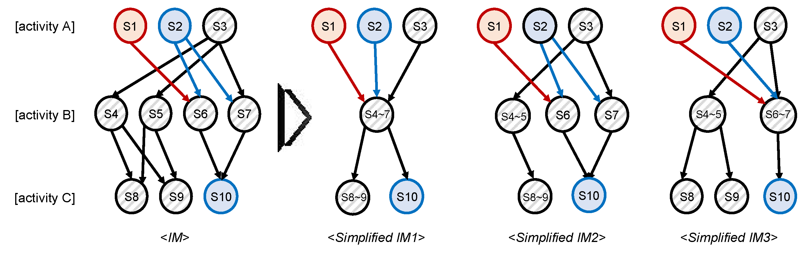
The final phase of the proposed approach is the model simplification based on the integrated context-aware resource model from Section 3.4 and the state properties from Section 3.5. As discussed earlier, the moderate states that belong to the same activity are merged with a specific condition. In this paper, we provide three types of conditions, and they are introduced in Definition 6.
Definition 6.
(Merging). Let be a transition system. Let be the target states that belong to the same activity, i.e., . Let be a moderate set. States can be merged if they hold the following conditions.
- -
- Type 1: All states belong to the moderate set M, i.e., .
- -
- Type 2: All states belong to the moderate set M, i.e., , and all events that enter into have the same property (where, the event property includes superior, inferior, and moderate).
- -
- Type 3: All states belong to the moderate set M, i.e., , and all events that come out from have the same property (where, the event property includes superior, inferior, and moderate).
The first type of merging is to combine all moderate states in a simple way. For example, if some of the states that are relevant to the same activity have a moderate property, those are straightforwardly combined into one moderate state. This approach, however, neglects the performance of arcs presented in Section 3.4. The second or the third method considers both moderate states and the corresponding arc performances. In the second approach, only moderate states with the same incoming event property are merged into one. On the other hand, the third approach conducts merging when the outgoing event property is the same.
Figure 4 gives an example of how to simplify models based on three different merging conditions. The default model IM has 10 states for three activities, i.e., A, B, and C. Here, if the first type is applied, as depicted in Simplified IM1, all states in activity B are merged into one state S4−7, and some of the states, i.e., S8 and S9 in activity C are combined. If the second type is chosen, we should check whether the property of incoming states is the same. For example, in activity B of Simplified IM2, only S4 and S5 have the neutral incoming event property, while others have different ones. Then, only S4 and S5 can be merged into one state, i.e., S4−5. If we consider the third option, S4−5 and S6−7 can be created as presented in Simplified IM3. This is because the property of outgoing events are the same as each other.
4. Implementation
This section first introduces the architecture of the implemented tool for mining a quality-aware resource model. Then, we present how to visualize the result of the proposed approach in an effective manner.
4.1. Architecture
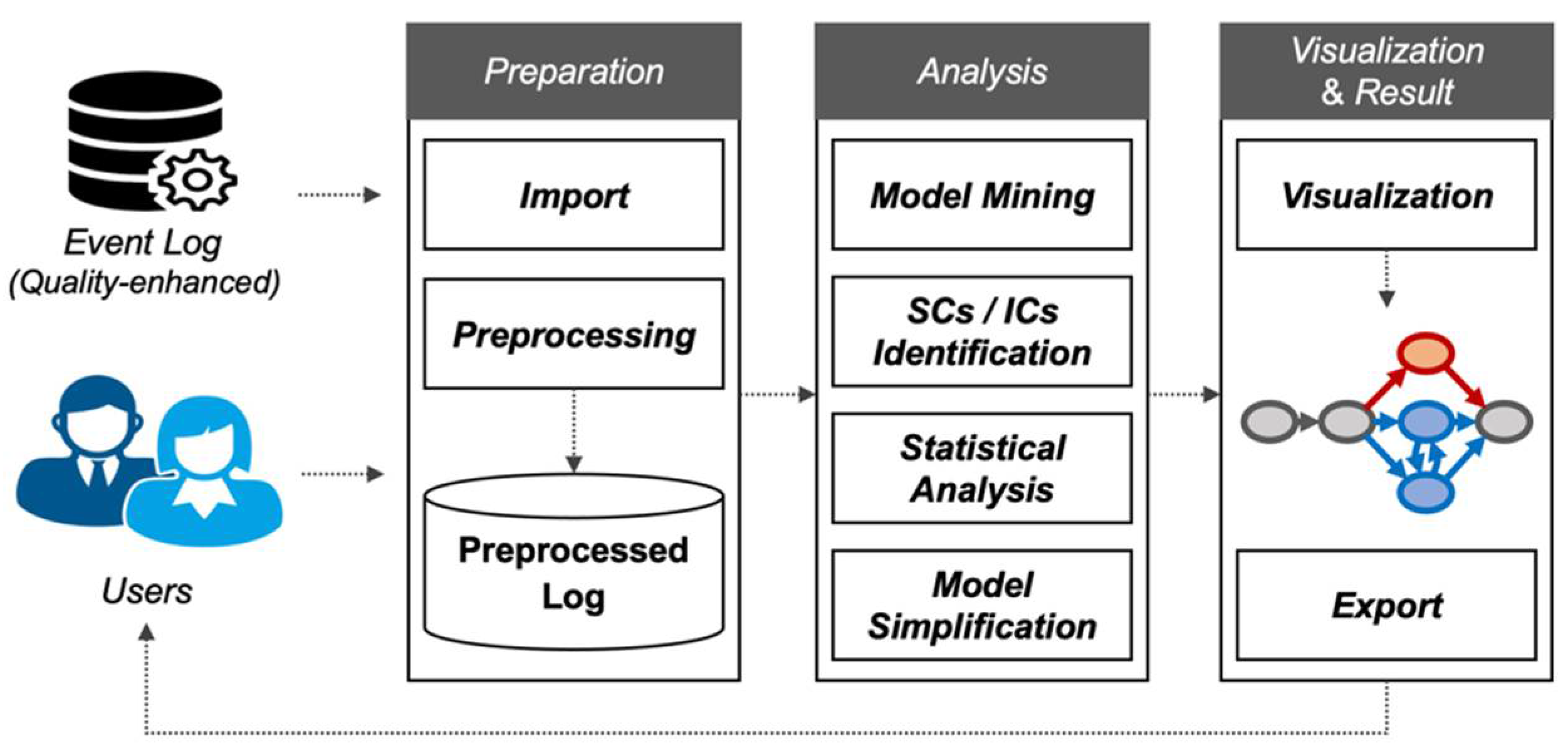
Our approach has been implemented as a Python application with an easy-to-use graphical user interface. Figure 5 depicts the architecture of the implemented tool, and it is composed mainly of three layers: Preparation, Analysis, and Visualization and Result. Each layer has several modules which perform specific roles.
The preparation layer has a role in preparing the data suitable for applying the proposed method. This layer is composed of the Import module, which loads event logs into the implemented tool and the Preprocessing module that performs preprocessing methods such as data error and imperfect data handling.
The analysis layer is the main component in our architecture that performs our approach, including discovering transition systems, the superior and inferior case identification, and model simplification. The Model Mining module produces a transition system from the preprocessed event log with the selected state and event representation functions. The SCs/ICs Identification module classifies cases into the superior, inferior, and moderate groups with user’s involvement. The Statistical Analysis module determines what resources are included in the superior, inferior, and moderate class based on the correlation with the quality, respectively. Lastly, the Model Simplification module streamlines the model for clear visualization.
The visualization and result layer presents the final outcomes to users. The Visualization module creates the interactive viewer, composed of filtering and highlighting capabilities, and envisions the outcomes to be delivered. The Export module helps to save the network for later usage.
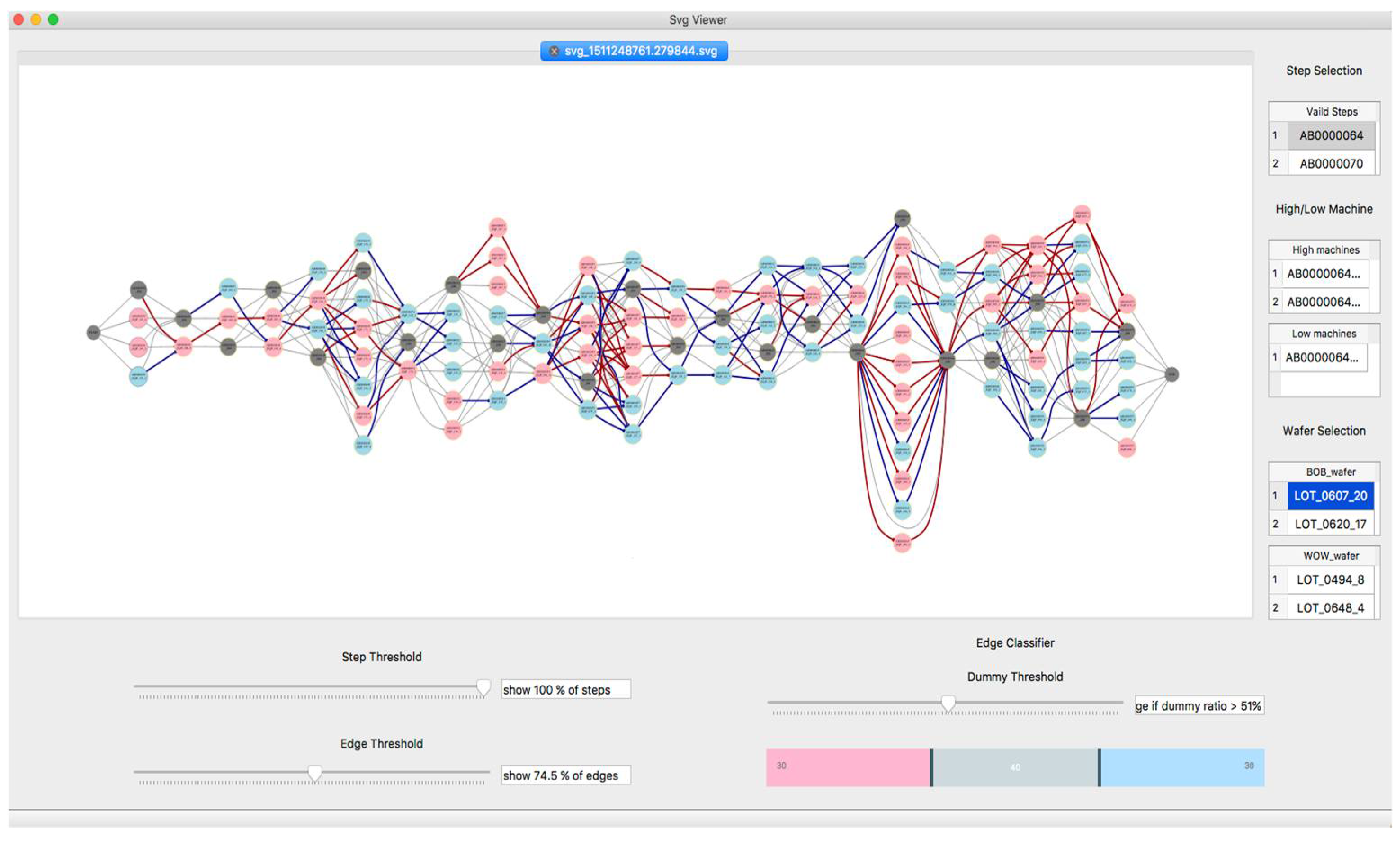
Our tool provides a graphical user interface, i.e., GUI, to achieve user-friendliness. Users deliver the required parameters through GUI, which are defined in our methods, including preprocessing options, state and event representation functions, statistical parameters, and simplification options. In addition, in the interactive visualization panel, filtering and highlighting methods are provided with GUI to provide more precise visualization, allowing users to fine-tune the complexity of the resulting model. Figure 6 presents the example of the visualization panel of the implemented tool. The derived result is shown at the top of the panel, and filtering and highlighting options are placed at the bottom. Based on these options, the model can be simplified and effectively visualized. The details for the visualization of the model are provided in Section 4.2.
4.2. Visualization
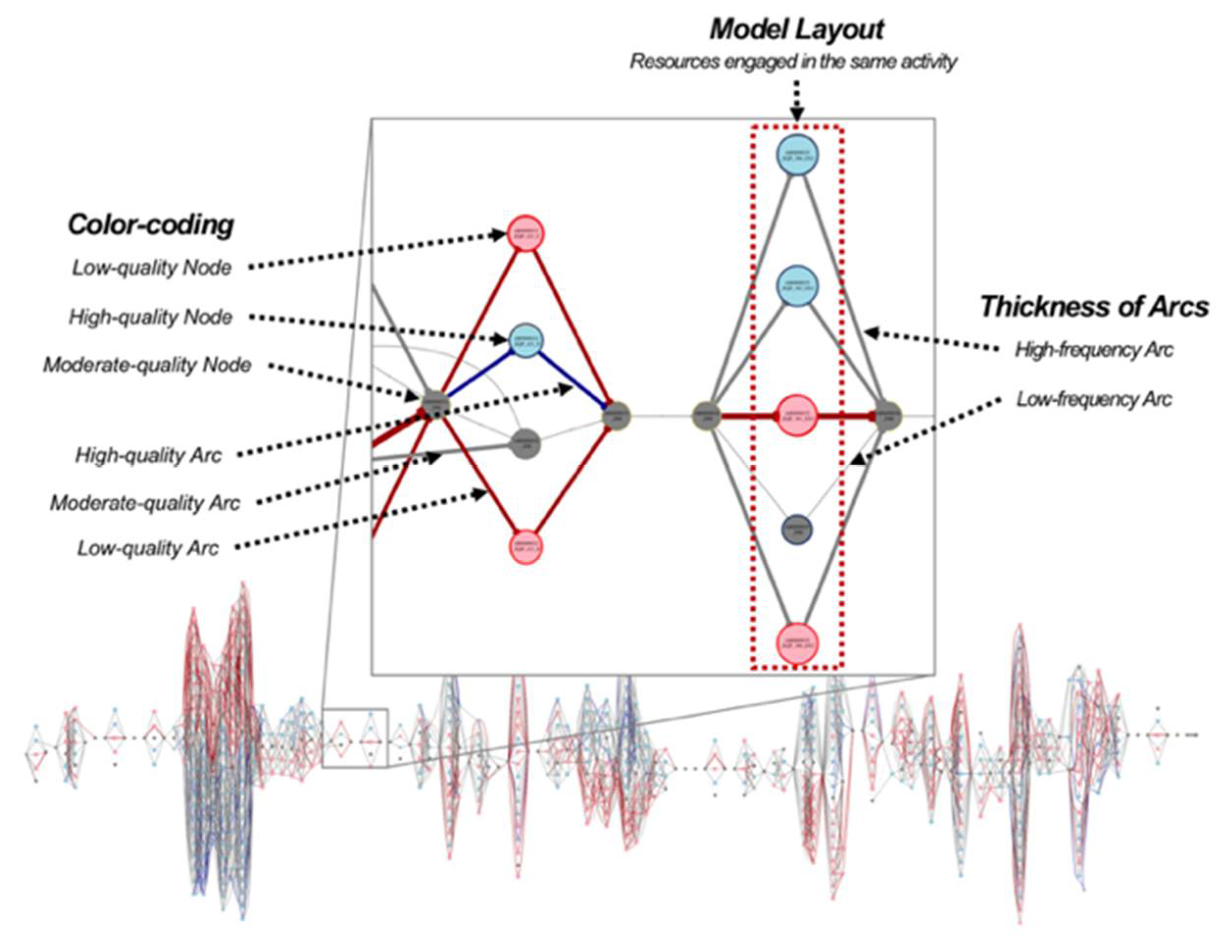
As discussed earlier, it is essential the derived model is effectively visualized for the model-based analysis. This section introduces three elements exploited for enhanced visualization in the implemented tool: the model layout, color-coding, and thickness of arcs. Figure 7 provides the visualization details of the derived model.
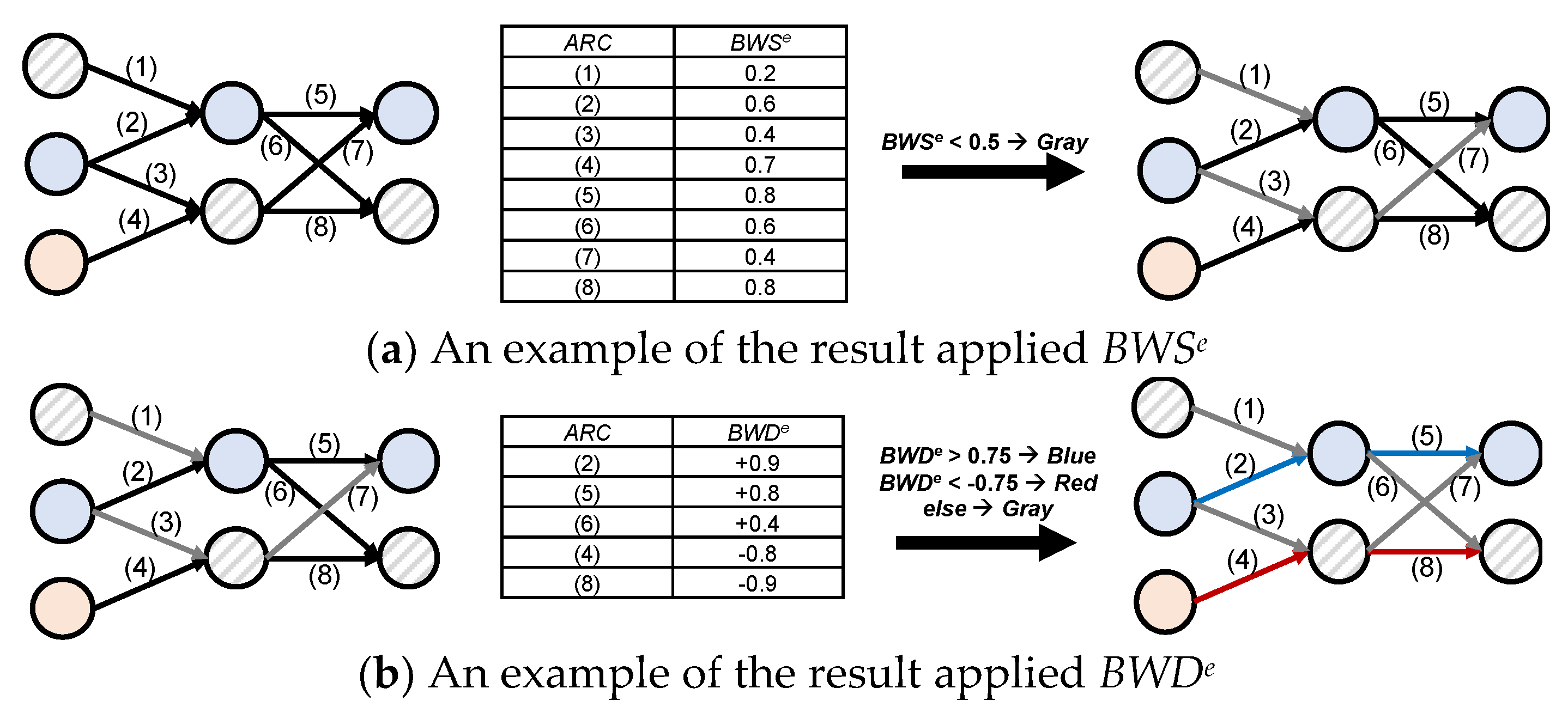
In the implemented tool, it is required that color-coding is applied to highlight three elements in the model: arcs, border of nodes, and inside of nodes. The color of arcs illustrates how many superior or inferior cases have passed through the corresponding arcs. As far as the color of arcs is concerned, we utilize BWSe and BWDe defined in Section 3.4. First, it is determined that a specific arc is significant compared to the other arcs with BWSe. Here, the arcs that have lower BWSe than the user-defined threshold are coded to gray. Note that BWSe has a range from 0 to 1. The rest of the arcs, i.e., the arcs with higher BWSe, are evaluated whether they have a positive or a negative effect on the quality with BWSe. In more detail, the arcs that have higher or lower BWDe than the two different thresholds are painted in blue and red, respectively. Note that BWDe has a range from −1 to 1. Figure 8 provides an example of the model that applied the color-coding. In this example, the user-defined criteria for BWSe are 0.5, while those for BWDe are 0.75 (for blue) and −0.75 (for red), respectively. In Figure 8a, the BWSe values of arcs (1), (3), and (7) are less than 0.5; thus, they are painted to gray, as shown in the model on the right. Then, the BWDe values are calculated for the remaining arcs, and they are evaluated with the predefined thresholds. In Figure 8b, we can identify that the arcs (2) and (5) are presented as blue in color, i.e., their values are higher than 0.75. Contrariwise, the arcs (7) and (8) have lower BWDe values than −0.75, and they are coded into red. The resulting model is depicted on the right of Figure 8b.
Similar to the arc, the color in the border of nodes indicates how many of the superior or inferior cases go through the states that the corresponding nodes represent. The procedure to determine the color is analogous to the one described in the arc highlighting, whereas we now employ BWSs and BWDs. The inside color of nodes is established with the statistical results on machines proposed in Section 3.5.
Lastly, the thickness of the arc denotes how many transitions occur through particular states; thus, the broader the arcs are, the higher the frequency of arcs. We employed the Equation (1) [27] to determine the thickness of arcs.
Given an ATS = (), assume that xij denotes the frequency of the transition and yij denotes the degree of thickness of the arc that connects si and sj. Then, the thickness of the arc yij is determined with the following values: the minimum and maximum frequency of transitions, i.e., xmin and xmax, and the user-defined minimum and maximum of the arc thickness, i.e., ymin and ymax. Note that yij becomes ymin or ymax as xij gets closer to xmin or xmax.
5. Evaluation
To demonstrate the usefulness of the proposed methodology, we conducted a case study with a real-life manufacturing event log. The goal of this evaluation was to diagnose whether the sound and poor resource paths in a manufacturing process could be determined based on our approach.
5.1. Design
The case study was conducted at a manufacturing company in Korea producing a variety of semiconductor products. According to the confidentiality agreements, we cannot present the details on the semiconductor manufacturing process utilized for this case study. In short, we can understand it as an ordinary semiconductor manufacturing process consisting of more than 500 sub-activities such as wafer fabrication, oxidation, photolithography, and etching. In addition, the process had a complicated resource network model because of the lengthy process and too many resources involved.
To evaluate the effectiveness of our approach in the manufacturing process, we answered the following research questions:
- -
- Is it able to identify the superior and inferior resource paths using the real-life manufacturing event logs?
- -
- Is the model simplification based on the quality of resources useful for a better understanding?
We extracted a quality-enhanced manufacturing event log from the manufacturing information systems supporting the execution of the corresponding process. The event log included approximately 15,000 wafers, i.e., process instances. From all of the 500 sub-activities, we collected 118 activities to be analyzed with the help of domain experts. In addition, in this case study, we utilized the quality, i.e., qualified outputs of all the produced wafers as quality measurements, and it had a range from 0 to 1.
5.2. Results
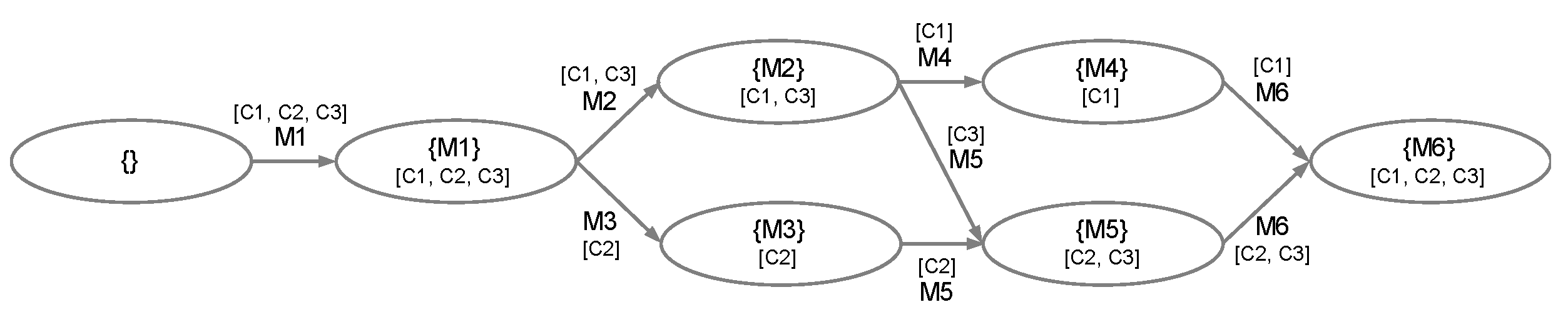
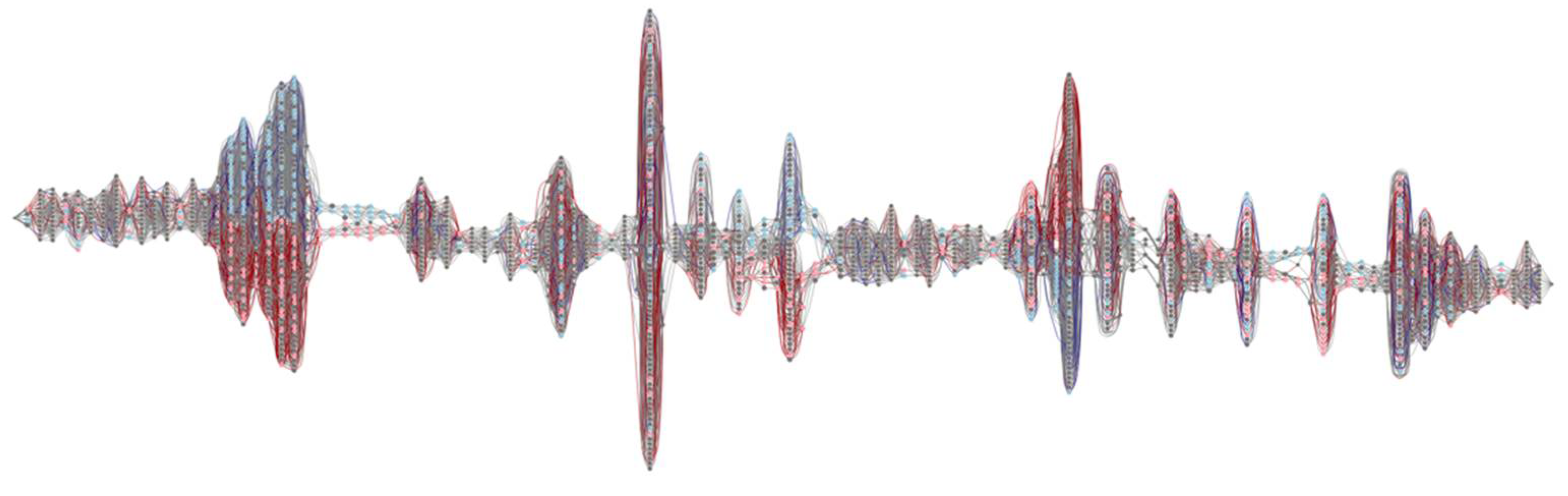
First, we discovered a transition system from the collected event log with an abstraction such that: and . After that, we identified the superior and inferior cases by applying the user-defined weight as 0.85; thus, we obtained 20% of the superior and inferior cases, respectively. Figure 9 depicts the model that integrates the derived transition system and the superior and inferior cases.
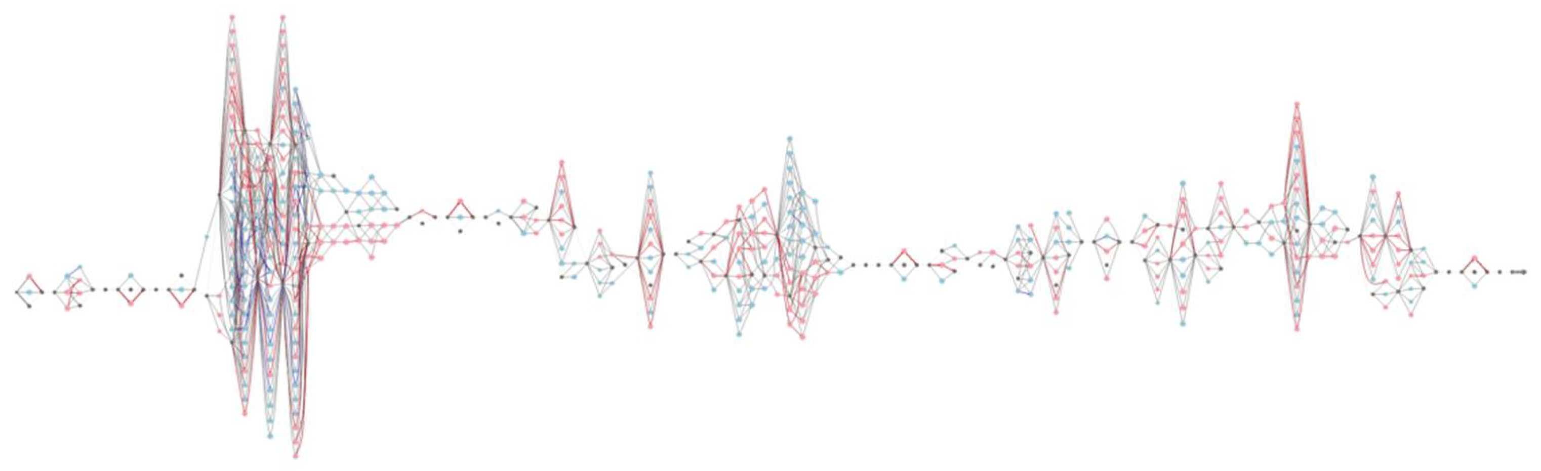
According to the number of activities included in the log, the integrated model had 120 vertical lines (i.e., 118 activities and artificial start and end), which included multiple states, i.e., manufacturing resources. For example, in the leftmost vertical line, four resources were engaged: one blue, one red, and two gray nodes. After that, we performed the rest of the proposed methodology, i.e., statistical analysis with all significance level thresholds as 0.05 and model simplification with simplifiedIM1. Figure 10 presents the quality-based simplified resource model.
Similar to Figure 9, we could recognize that Figure 10 was also composed of 120 vertical lines. However, the number of states for each line was dramatically decreased in this figure. For example, in the 51st line, i.e., the longest vertical line in Figure 9, the number of states became 12, while it was 93 in the previous figure. Furthermore, it was discovered what resources had a significant effect on the quality in each activity. In the 51st activity, six resources displayed as blue nodes, produced high quality, while five resources, i.e., the red nodes, were connected to poor quality. Note that the corresponding nodes had statistically significant effects on quality compared to other ones.
5.3. Discussion
Based on the results of applying the proposed approach to the manufacturing log, we answered the two presented questions. First, we showed the applicability of our approach by providing the model-based analysis results to identify the superior and inferior resource paths. In a nutshell, we determined the important resource paths on quality, and that they can be applied for manufacturing planning or operating. Second, we employed several metrics to evaluate the complexity of models, such as the number of nodes and arcs for validating the effectiveness of the model simplification. The number of nodes and arcs was calculated for the model as a whole. As a result, we were able to notice that Figure 10 is much simpler than Figure 9. The number of nodes and arcs was remarkably decreased with 71.6% (i.e., from 1773 to 504) and 91% (i.e., from 11,973 to 1078), respectively. Therefore, we concluded that model simplification is helpful in a quantitative context. In addition, we were convinced that the simplified model is remarkably effective because it focused on essential resources on quality, unlike the previous model that visualized all of the behaviors.
6. Conclusions
This paper suggested a method to derive a quality-aware resource model. In this regard, we employed a model discovery algorithm, i.e., transition system, and a series of statistical approaches. In addition, we provided tooling support for the proposed approach, and the manufacturing case study was presented to validate our approach. As a result, we identified that our approach is effective in understanding the relationship between resource paths and quality.
This study has the strength of employing transition systems, i.e., one of low-level process models, which perfectly fit the event log and so we do not need to validate the model from the behavior perspective. Transition systems define states and transitions from event logs as they are, instead of discovering control-flows, such as OR-split/join and AND-split/join. Thus, the model holds all of the behavior in event logs. In addition, our approach allows model simplification. However, this is a process of integrating and replacing the resources into a dummy that does not affect the quality, rather than a filtering process that removes specific resources from the model. Thus, we can determine that the model fits the log by comparing the simplified model and the traces replaced by dummy resources.
Regarding the quality perspective as well as the behavior, we need to consider a couple of viewpoints for the validation: (i) whether the process instances from the model are well predicted as high or low quality and (ii) whether the resources engaged in each activity are well-segmented as the high- or low-quality group. To validate the first viewpoint, we can employ the general validation method for supervised learning classification tasks, i.e., dividing the event log into training and validation datasets and evaluating the model by comparing the actual and the predicted results with a confusion matrix. As far as the second viewpoint is concerned, in the process of the statistical analyses on resources, we already use the p-value to support the significance of the results. That is, we can argue that the model performs the validation itself. In addition to this, we plan to build a systematic validation method to improve the completeness of the proposed approach through future work.
This work has several limitations. First, our approach is relatively automated, but it still requires user intervention, e.g., user-specified weights. In other words, our approach partly depends on practitioners in a specific domain for better modeling and visualization. Therefore, future research should deal with how to derive the optimal parameters for a particular process. In addition, our approach effectively understands the relationship between resource paths and quality, but it does not hold the ability to predict the quality for a specific case. We need to develop a method to predict the quality value based on resource paths and other attributes. Furthermore, we should extend our approach to an online-fashioned method based on real-time data that estimates quality and recommends the optimized resource paths at the moment the process is running.
As future works, we will conduct research to construct a model that reflects the states of the resources based on the other data, e.g., sensor data, and that have a relationship with quality. Furthermore, we will develop a method to present our approach in an online setting and predict the quality of cases. In addition, we have a plan to conduct more case studies with other domains, e.g., healthcare and service sectors.
Author Contributions
Methodology, software, and formal analysis, All authors; writing—original draft preparation, M.C. and G.P.; writing—review and editing, M.S., J.L. and E.K.; supervision, M.S. All authors have read and agreed to the published version of the manuscript.
Funding
This work was supported by the Research Program from Samsung Electronics Company Ltd. and the Korea Institute for Advancement of Technology (KIAT) grant funded by the Korean Government (MOTIE) (N0008691, The Competency Development Program for Industry Specialists).
Institutional Review Board Statement
Not applicable.
Informed Consent Statement
Not applicable.
Conflicts of Interest
The authors declare no conflict of interest.
References
- van der Aalst, W.M.P. Data Science in Action. In Process Mining; Publisher Springer: Heidelberg, Germany, 2016. [Google Scholar]
- Reinkemeyer, L. Process Mining in Action: Principles, Use Cases and Outlook; Publisher Springer: Cham, Switzerland, 2020. [Google Scholar]
- Shraga, R.; Gal, A.; Schumacher, D.; Senderovich, A.; Weidlich, M. Process discovery with context-aware process trees. Inf. Syst. 2020, 101533. [Google Scholar] [CrossRef]
- Marquez-Chamorro, A.; Revoredo, K.; Resinas, M.; Del-Rio-Ortega, A.; Santoro, F.; Ruiz-Cortes, A. Context-Aware Process Performance Indicator Prediction. IEEE Access 2020, 8, 222050–222063. [Google Scholar] [CrossRef]
- Hompes, B.; Buijs, J.; van der Aalst, W. A Generic Framework for Context-Aware Process Performance Analysis. In Proceedings of the On the Move to Meaningful Internet Systems: OTM 2016 Conferences, Rhodes, Greece, 24–28 October 2016; pp. 300–317. [Google Scholar]
- Huang, Z.; Lu, X.; Duan, H. Resource behavior measure and application in business process management. Expert. Syst. Appl. 2012, 39, 6458–6468. [Google Scholar] [CrossRef]
- Cho, M.; Park, G.; Song, M.; Lee, J.; Lee, B.; Kim, E. Discovery of Resource-oriented Transition Systems for Yield Enhancement in Semiconductor Manufacturing. IEEE Trans. Semicond. Manuf. 2021, 34, 17–24. [Google Scholar] [CrossRef]
- Cho, M.; Song, M.; Comuzzi, M.; Yoo, S. Evaluating the effect of best practices for business process redesign: An evidence-based approach based on process mining techniques. Decis. Support Syst. 2017, 104, 92–103. [Google Scholar] [CrossRef]
- Graafmans, T.; Turetken, O.; Poppelaars, H.; Fahland, D. Process Mining for Six Sigma. Bus. Inf. Syst. Eng. 2020, 63, 277–300. [Google Scholar] [CrossRef]
- Samson, D.; Terziovski, M. The relationship between total quality management practices and operational performance. J. Oper. Manag. 1999, 17, 393–409. [Google Scholar] [CrossRef]
- Garcia, C.; Meincheim, A.; Faria Junior, E.; Dallagassa, M.; Sato, D.; Carvalho, D.; Santos, E.; Scalabrin, E. Process mining techniques and applications—A systematic mapping study. Expert. Syst. Appl. 2019, 133, 260–295. [Google Scholar] [CrossRef]
- van der Aalst, W.M.P.; Schonenberg, M.; Song, M. Time prediction based on process mining. Inf. Syst. 2011, 36, 450–475. [Google Scholar] [CrossRef] [Green Version]
- Hong, T.; Song, M. Analysis and Prediction Cost of Manufacturing Process Based on Process Mining. In Proceedings of the 2016 International Conference on Industrial Engineering, Management Science and Application (ICIMSA), Jeju Island, Korea, 23–26 May 2016. [Google Scholar]
- Rozinat, A.; van der Aalst, W. Decision Mining in ProM. In Lecture Notes in Computer Science; Springer: Berlin/Heidelberg, Germany, 2006; pp. 420–425. [Google Scholar]
- Mannhardt, F.; de Leoni, M.; Reijers, H.; van der Aalst, W. Balanced multi-perspective checking of process conformance. Computing 2015, 98, 407–437. [Google Scholar] [CrossRef] [Green Version]
- Burattin, A.; Maggi, F.; Sperduti, A. Conformance checking based on multi-perspective declarative process models. Expert. Syst. Appl. 2016, 65, 194–211. [Google Scholar] [CrossRef] [Green Version]
- Maggi, F.; Montali, M.; Bhat, U. Compliance Monitoring of Multi-Perspective Declarative Process Models. In Proceedings of the 2019 IEEE 23rd International Enterprise Distributed Object Computing Conference (EDOC), Paris, France, 28–30 October 2019. [Google Scholar]
- Bose, R.; van der Aalst, W. Context Aware Trace Clustering: Towards Improving Process Mining Results. In Proceedings of the 2009 SIAM International Conference on Data Mining, Sparks, NV, USA, 30 April–2 May 2009. [Google Scholar]
- van der Aalst, W.M.P. The Application of Petri Nets to Workflow Management. J. Circuits Syst. Comput. 1998, 8, 21–66. [Google Scholar] [CrossRef] [Green Version]
- van der Aalst, W.M.P.; ter Hofstede, A. YAWL: Yet another workflow language. Inf. Syst. 2005, 30, 245–275. [Google Scholar] [CrossRef] [Green Version]
- Dijkman, R.; Dumas, M.; Ouyang, C. Semantics and analysis of business process models in BPMN. Inf. Softw. Technol. 2008, 50, 1281–1294. [Google Scholar] [CrossRef] [Green Version]
- Ghasemi, A.; Zahediasl, S. Normality Tests for Statistical Analysis: A Guide for Non-Statisticians. Int. J. Endocrinol. Metab. 2012, 10, 486–489. [Google Scholar] [CrossRef] [PubMed] [Green Version]
- Leys, C.; Ley, C.; Klein, O.; Bernard, P.; Licata, L. Detecting outliers: Do not use standard deviation around the mean, use absolute deviation around the median. J. Exp. Soc. Psychol. 2013, 49, 764–766. [Google Scholar] [CrossRef] [Green Version]
- Hothorn, T.; Bretz, F.; Westfall, P. Simultaneous Inference in General Parametric Models. Biom. J. 2008, 50, 346–363. [Google Scholar] [CrossRef] [PubMed] [Green Version]
- Smyth, G. Linear Models and Empirical Bayes Methods for Assessing Differential Expression in Microarray Experiments. Stat. Appl. Genet. Mol. Biol. 2004, 3, 1–25. [Google Scholar] [CrossRef] [PubMed]
- Corder, G.; Foreman, D. Nonparametric Statistics for Non-Statisticians; Wiley: Hoboken, NJ, USA, 2011. [Google Scholar]
- Ferreira, D. Primer on Process Mining; Springer Nature: Basingstoke, UK, 2020. [Google Scholar]
Figure 1.
Overview of the proposed approach.

Figure 2.
Examples of transition systems based on the event log in Table 1.
Figure 2.
Examples of transition systems based on the event log in Table 1.


Figure 3.
An example of the case-annotated transition systems () with and based on the event log in Table 1.
Figure 3.
An example of the case-annotated transition systems () with and based on the event log in Table 1.

Figure 4.
An Example of the simplified models with different conditions.

Figure 5.
The architecture of the implemented tool.

Figure 6.
The interactive viewer in the implemented tool.

Figure 7.
Visualization details of the model.

Figure 8.
An example of the model that applied the arc color-coding.

Figure 9.
The integrated model from the collected manufacturing log.

Figure 10.
The simplified model from the collected manufacturing log with the statistical analysis.


Table 1.
A snippet of event logs.
| CaseID | Event | Activity | Originator | Timestamp | Attribute (Quality) |
|---|---|---|---|---|---|
| C1 | E1 | A | M1 | 1 January 2021 10:30 | 0.95 |
| C1 | E2 | B | M2 | 1 January 2021 12:00 | 0.95 |
| C1 | E3 | C | M4 | 1 January 2021 17:00 | 0.95 |
| C1 | E4 | D | M6 | 2 January 2021 09:00 | 0.95 |
| C2 | E5 | A | M1 | 4 January 2021 09:00 | 0.85 |
| C2 | E6 | B | M3 | 4 January 2021 12:00 | 0.85 |
| C2 | E7 | C | M5 | 4 January 2021 15:00 | 0.85 |
| C2 | E8 | D | M6 | 5 January 2021 13:00 | 0.85 |
| C3 | E9 | A | M1 | 6 January 2021 09:00 | 0.9 |
| C3 | E10 | B | M2 | 6 January 2021 14:00 | 0.9 |
| C3 | E11 | C | M5 | 7 January 2021 13:00 | 0.9 |
| C3 | E12 | D | M6 | 7 January 2021 18:00 | 0.9 |
Publisher’s Note: MDPI stays neutral with regard to jurisdictional claims in published maps and institutional affiliations. |
© 2021 by the authors. Licensee MDPI, Basel, Switzerland. This article is an open access article distributed under the terms and conditions of the Creative Commons Attribution (CC BY) license (https://creativecommons.org/licenses/by/4.0/).
Share and Cite
MDPI and ACS Style
Cho, M.; Park, G.; Song, M.; Lee, J.; Kum, E. Quality-Aware Resource Model Discovery. Appl. Sci. 2021, 11, 5730. https://0-doi-org.brum.beds.ac.uk/10.3390/app11125730
AMA Style
Cho M, Park G, Song M, Lee J, Kum E. Quality-Aware Resource Model Discovery. Applied Sciences. 2021; 11(12):5730. https://0-doi-org.brum.beds.ac.uk/10.3390/app11125730
Chicago/Turabian StyleCho, Minsu, Gyunam Park, Minseok Song, Jinyoun Lee, and Euiseok Kum. 2021. "Quality-Aware Resource Model Discovery" Applied Sciences 11, no. 12: 5730. https://0-doi-org.brum.beds.ac.uk/10.3390/app11125730
Note that from the first issue of 2016, this journal uses article numbers instead of page numbers. See further details here.