Complex Systems, Emergence, and Multiscale Analysis: A Tutorial and Brief Survey

Abstract

Mankind has long been fascinated by emergence in complex systems. With the rapidly accumulating big data in almost every branch of science, engineering, and society, a golden age for the study of complex systems and emergence has arisen. Among the many values of big data are to detect changes in system dynamics and to help science to extend its reach, and most desirably, to possibly uncover new fundamental laws. Unfortunately, these goals are hard to achieve using black-box machine-learning based approaches for big data analysis. Especially, when systems are not functioning properly, their dynamics must be highly nonlinear, and as long as abnormal behaviors occur rarely, relevant data for abnormal behaviors cannot be expected to be abundant enough to be adequately tackled by machine-learning based approaches. To better cope with these situations, we advocate to synergistically use mainstream machine learning based approaches and multiscale approaches from complexity science. The latter are very useful for finding key parameters characterizing the evolution of a dynamical system, including malfunctioning of the system. One of the many uses of such parameters is to design simpler but more accurate unsupervised machine learning schemes. To illustrate the ideas, we will first provide a tutorial introduction to complex systems and emergence, then we present two multiscale approaches. One is based on adaptive filtering, which is excellent at trend analysis, noise reduction, and (multi)fractal analysis. The other originates from chaos theory and can unify the major complexity measures that have been developed in recent decades. To make the ideas and methods better accessed by a wider audience, the paper is designed as a tutorial survey, emphasizing the connections among the different concepts from complexity science. Many original discussions, arguments, and results pertinent to real-world applications are also presented so that readers can be best stimulated to apply and further develop the ideas and methods covered in the article to solve their own problems. This article is purported both as a tutorial and a survey. It can be used as course material, including summer extensive training courses. When the material is used for teaching purposes, it will be beneficial to motivate students to have hands-on experiences with the many methods discussed in the paper. Instructors as well as readers interested in the computer analysis programs are welcome to contact the corresponding author.

1. Introduction

The ever increasing amount of big data in science, engineering, and society, including meteorological, hydrological, ecological, environmental, as well as various kinds of biomedical, manufacturing, e-commerce, and government management data, has fueled enormous optimism among researchers, entrepreneurs, government officials, the media, and the general public [1,2]. It is now hoped that by recording and analyzing the errors of all the components of a sophisticated machine, one can quickly diagnose and then fix its malfunctioning. When one is sick, one hopes that in the near future, with all the increasingly detailed data about oneself, including genomic, cellular, clinical, psychological, and environmental data, one may promptly get optimized treatment. One also hopes to identify the most promising stocks by collecting and analyzing all the relevant economic data and then investing on them.

Such optimism is not entirely unfounded, as big data indeed has brought some pleasant surprises to science and society. For example, a good online shopping system can quickly and fairly accurately infer what an online shopper is looking for by analyzing the shopper’s online behavior in real time. By analyzing the tweets about major natural disasters, key information of disasters can be accurately obtained [3]. Google Flu Trends did an impressive job in predicting the 2008 influenza [4].

While the big data showcase does not stop at the above successful examples, it is important that one is not carried away by those successes. In fact, many more not so successful cases also exist. For example, right after 2008, Google Flu Trends over-predicted influenza outbreaks, and by 2012, the error was by as much as a factor of two [5], which then prompted Google to give up the predictor. The box office price of the film “Golden Times”, which was first released in China during the National Holiday, 1 October 2014, was only slightly more than 40 million, while Baidu, the leading Chinese web services company, predicted it to be about 200–230 million. The poor prediction by Baidu made a reviewer of the film to lament that big data may not be dependable [6]. Of course, we have to add the failed prediction of the Trump presidency in 2016 by many predictors, whose implications to the Americas, and even the world’s politics, are almost unfathomable.

Among the most important values of big data analysis are to detect changes in system dynamics (e.g., detect and understand abnormal behaviors ) and to help science to extend its reach (and most desirably, to possibly uncover new fundamental laws). This includes timely diagnosis and treatment of various kinds of diseases in health care, proper prediction of regime changes in weather and climate patterns, timely forewarning of natural disasters, and timely detection and fixing of malfunctioning of various kinds of devices, infrastructure, and software in the field of operation and maintenance [7,8,9,10], among many others. Understandably, abnormal behaviors cannot be expected to occur frequently, and thus the relevant data may not be so abundant that direct application of machine-learning based approaches will always be very rewarding. In those situations, the systems often generate data with complex characteristics including long-range spatial–temporal correlations, extreme variations (sometimes caused by small disturbances), time-varying mean and variance, and multiscale analysis (i.e., different behavior depending on the scales at which the data are examined). Such situations have been increasingly manifesting themselves in science, engineering, and society. To adequately cope with these situations, it is often beneficial to resort to complexity science to analyze the relevant data. In fact, when dealing with such highly challenging situations, many analyses using machine-learning based approaches may be considered pre-processing of the data or the first step that can facilitate further application of complexity-based approaches, or as post-processing of the features obtained through multiscale analysis. An excellent article along this line (more precisely, study of segmental organization of the human genome by combining complexity with machine learning approaches) has recently been reported by Karakatsanis et al. [11]. In short, the complex behaviors in nature, science, engineering, and society must be infinite. To help one to peek into the infinity of the complex behaviors, going beyond statistical analysis and machine-learning by resorting to the type of mathematics that embodies an element of infinity will often be beneficial.

At this point, it is important to pause for a moment to discuss a peculiar phenomenon: while many consider complexity science to be very useful, some others doubt its relevance to reality. Why is this so? The basic reason is that in complexity research, conceptual thinking, simulational study, and applications have not been well connected. For example, Science magazine dedicated the April 1999 issue to Complex Systems. A number of leading experts in their respective fields, including chemistry, physics, economics, ecology, and biology, expressed their views on the relevance/importance of complexity science in their fields. While the special issue is influential in making some concepts of complex systems known to a wider research community and even the general public, it does little in teaching readers how to solve real-world problems. This may have contributed to the waning of enthusiasm in complexity science research in the subsequent years, as most readers cannot see how complexity science can help solve their problems. Fortunately, the tide appears to have been reversed (please see recent reviews on complexity theory and leadership practice [12] and health [13]).

The purpose of this article is to convey how the many concepts in complexity science can be effectively applied to help one formulate stimulating problems pertinent to the data and the underlying system. We will particularly focus on multiscale approaches. They are the key to find scaling laws from the data. With the scaling laws, we can then find defining parameters/properties of the data and eliminate spurious causal relations in the data. The latter can help to shed some light on a new generation of AI, which is based on correlation/causality rather than pure probabilistic thinking [14]. To better serve our goal, we will discuss various kinds of applications right after a concept/method is introduced. Our goal here is to fully arouse readers’ interest in the materials covered, and to equip them with a set of widely applicable concepts and methods to help solve their own interesting problems.

2. Basics of Complex Systems and Emergence

2.1. Complex Systems and Emergence: Working Definitions

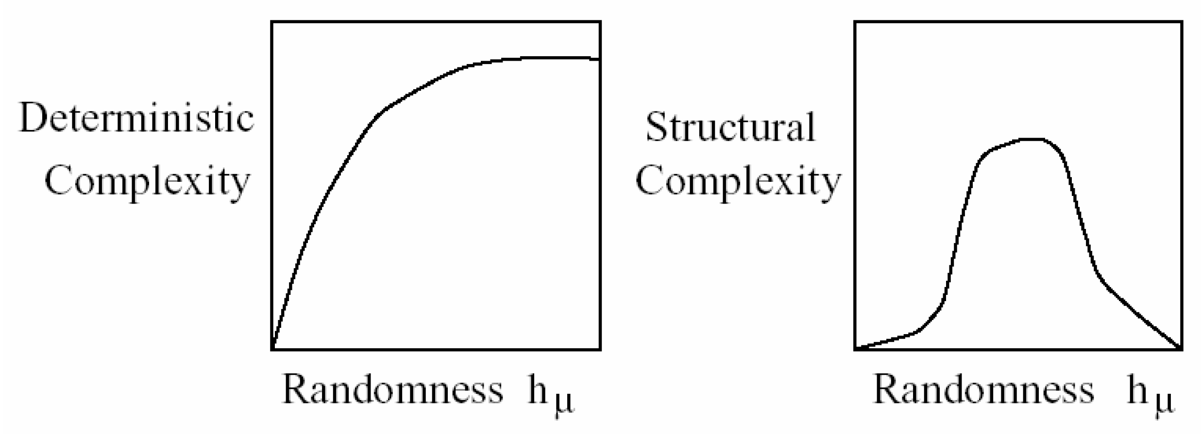
To better understand which systems can be considered complex, we first explain how complexity is quantified. There are two major types of measures. One is called Deterministic complexity, which increases with the degree of randomness. See Figure 1 (left). Widely used measures in this category include Shannon entropy [15], Kolmogorov–Sinai (KS) entropy [16,17], Kolmogorov–Chaitin complexity [18,19,20], and the Lempel–Ziv (LZ) complexity [21]. The other is called Structural complexity. Here, the measure attains a maximal value for an intermediate level of randomness. See Figure 1 (right).

Let us now examine the main features of a complex system. It is often thought that a complex system must consist of many interconnecting components or parts. The individual components together with their dynamics could be quite simple. The system as a whole, however, must exhibit complex dynamics. Note that with this view, a pendulum with chaotic behavior is no longer considered a complex system. In addition, note that some researchers (e.g., Kastens et al. [22]) advocate to assign a complex system with many more quantifiable features, such as feedback loops, multiple inputs and multiple outputs, non-Gaussian distributions of the outputs, nonlinear interactions, multiple stable states, fractal and chaotic behaviors, self-organized criticality, hierarchy, and so on. Our view is that it is extremely rare for a single system to simultaneously possess so many distinguished properties at the same time. Therefore, simpler definitions that give more room and freedom to think and work could be more beneficial.

Complex systems often defy pure statistical analysis. To illustrate the idea, let us discuss an author (JB)’s personal experience. JB worked at Guangxi University in Nanning for a few years. The campus was full of natural wonders, with flowers blossoming and many kinds of tropical and subtropical fruits dangling on trees all year long. Thus, JB and many of his friends truly enjoyed the campus. Approximately 100,000 people, including University employees and students, lived on campus. JB used to buy vegetables and meat at a farmer’s market in the east campus of the University. Although the farmer’s market was a bit shabby, it was in a convenient location and was visited by a lot of customers everyday. In the market, there was a pork meat seller who normally would sell out all the meat within 2.5 h before 11 am in the morning. Around October 2017, the market was relocated to a new place about 7 min walk from the original site. Surprisingly, the number of customers to the market dropped considerably. As a result, the pork meat seller would still be selling meat around 1–2 pm. After that, the seller had to take the meat to some fast food restaurants, as otherwise the pork, not refrigerated, would become spoiled and smelly. Surely, quite a few fruit and vegetable sellers eventually gave up. Such dramatic drop in customer number is very difficult to predict with statistical models, however sophisticated they are. One can readily see that to truly understand the phenomenon, one has to systematically analyze the dynamics of the customer behavior by considering diverse factors such as the variety, cost, and freshness of food; convenience of the market; competitors of the market; and customer psychology.

Next, let us consider emergence in complex systems. Emergence is a bulk property of the system involving many of the interacting components of the system [23,24]. As a result, its scale usually is much larger than that of the individual component. Outstanding examples of emergence include the spiral galaxy [25], the great red spot of Jupiter [26], hurricanes, tornadoes, phase transitions and critical phenomena [27], bird flocking [28,29], fish schooling [30,31,32,33], sand dunes [34], mass parades or protests, and bursts of anger (where many neurons in certain regions of the brain fire synchronously). Less frequently mentioned examples of emergence that are of tremendous significance to our society include the many innovations in technology, including Internet-enabled platform economy, where large numbers of sellers and buyers interact and transact through the platform. Among the important and fascinating questions concerning such platform-enabled emergent behaviors are to identify the conditions under which such services will become attractive and widely adopted, and to quantify the generic statistical properties underlying such services.

Often it is thought that for a system to exhibit an emergent behavior, it must have a hierarchical structure. This thinking is, however, not quite consistent with the fact that simple models with local interaction rules may simulate certain emergent behaviors quite well, including bird flocking and fish schooling [28,29,30,31,32,33].

We now consider Complex giant systems, a notion that has been widely discussed in many fields in China, including physics, mathematics, philosophy, and humanities. As fluid motions including turbulence are considered not to belong to such systems, social systems become the prototypical model here. While a big social system is certainly a giant system, as it contains so many individuals and their interactions, it is not necessarily a complex system. For example, in an autocratic state where governance is strictly hierarchical, from top to bottom, and all means of feedback, such as election, parade protests, and so on, are prohibited, the social dynamics of a specific layer are only directionally connected to its nearest upper and lower layers (driven and driving, respectively). This is the consequence of lacking a persistent negative feedback loop in the society. As a result, the complexities of such societies cannot be considered very high, as those societies do not possess well-developed dynamics that have to be enabled by feedback loops. In particular, they lack many emergent behaviors that a democratic society has, such as parade protests instigated by explosions in public opinion.

In the study of complex systems, different researchers may have different emphasis [35,36]. One school focuses on the mathematics and mechanics of complex systems. Here, one is mainly concerned about rigorous mathematical analysis of the system under study, most desirably starting from fundamental governing equations of the system, and using mechanics (quantum, classical, and statistical) to analyze the system. While in principle a living organism (e.g., the human body) may be modeled by a large set of differential equations with a lot of controlling parameters, with the values of the parameters indicating healthy or diseased states, this may not be achieved in the near future. To better exploit the unprecedented opportunities provided by the explosion of data in all areas of science, technology, and society, in this article we adopt a data-driven approach to study complex systems. Among the many techniques to analyze data is distribution analysis. As the power law is a distribution with many interesting properties that are not shared by most commonly used distributions in conventional statistical analysis, in the next subsection we will discuss the power law and the related heavy-tailed distributions.

2.2. Power Law and Heavy-Tailed Distributions

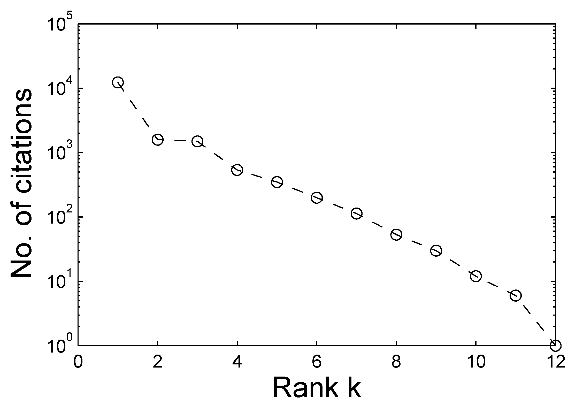
In contrast to Gaussian, exponential, and other thin-tailed distributions that have a well-defined scale, a power law distribution does not have a scale. It has been observed in various kinds of physical, biological, technological, and and social systems. Well-known examples include the distribution of word frequency, web hits, citations of scientific papers, telephone calls, copies of books sold, diameter of moon craters, intensity of solar flares, intensity of wars, magnitude of earthquakes, wealth of the richest people, and population of cities [37].

A power law distribution can be expressed by its probability density function (PDF) [38]

$$f\left(x\right)\sim x^{-\alpha -1},x\to \infty ,$$

(1)

or equivalently by the complementary cumulative distribution function (CCDF) [38]

$$P[X\ge x]\sim x^{-\alpha },x\to \infty .$$

(2)

Notice here the emphasis that $x\to \infty$. An interesting property of the power law distribution is that for a given $\alpha$, its moments with order higher than $\alpha$ do not exist. Therefore, when $0<\alpha <2$, the variance and all moments higher than the second order do not exist, and when $0<\alpha \le 1$, even the mean is infinite. When the power law relation extends to the entire range of the allowable x, we have the Pareto distribution [39]:

$$P[X\ge x]={\left(\frac{b}{x}\right)}^{\alpha },x\ge b>0,\alpha >0,$$

(3)

Here, $\alpha$ is the shape parameter, and b the location parameter. In the discrete case, the Pareto distribution is called the Zipf distribution, which provides an excellent description between the frequency of any word in a corpus of natural language and its rank in the frequency table.

Somewhat related to the Zipf distribution is another distribution called Benford’s law [40], which is about the probability of occurrence of leading digits $d\in \{1,2,\cdots ,9\}$,

$$P\left(d\right)={log}_{10}(d+1)-{log}_{10}\left(d\right)={log}_{10}\left(1+\frac{1}{d}\right)$$

(4)

A good mechanism for explaining the uneven distributions stipulated by Benford’s law has been proposed in [41].

Benford’s law has been used for evaluating possible fraud in accounting data [42], legal status [43], election data [44,45,46], macroeconomic data [47], price data [48], etc. From Equation (4), we observe that beyond the small digits, the probability approximately approaches the Zipf distribution with $\alpha =1$,

$$P\left(d\right)={log}_{10}\left(1+\frac{1}{d}\right)\sim d^{-1}/ln\left(10\right),d=3,4,\cdots ,9$$

(5)

2.2.1. Pareto Principle or the 80/20 Rule

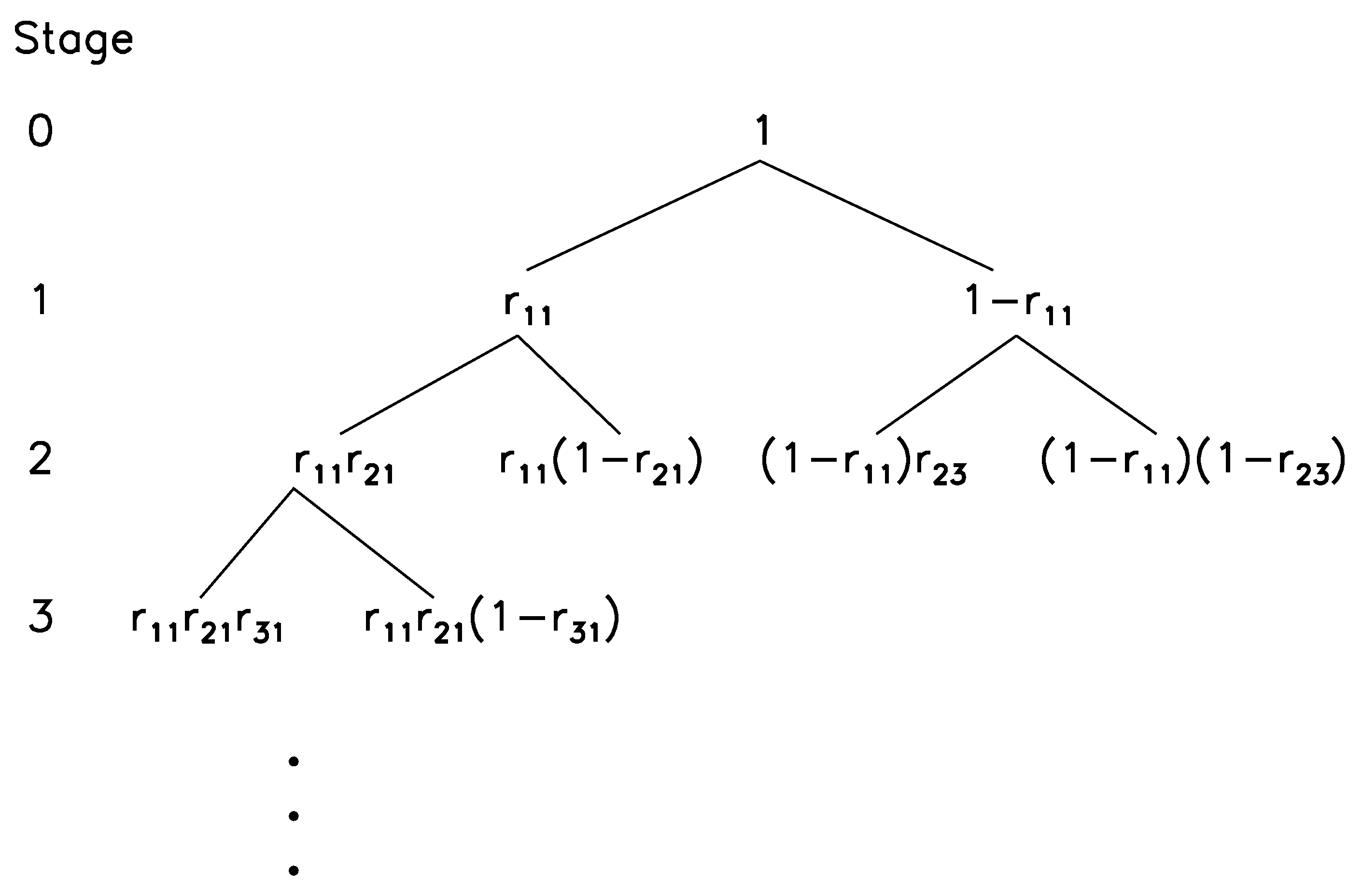
The 80/20 rule or the Pareto principle was first put foreword by the Italian economist Vilfredo Pareto in 1896: approximately 80% of the land in Italy was owned by 20% of the population. The rule later more generally applies, as approximately 80% of the wealth in a society is owned by 20% of the population. It can be derived from the Pareto distribution with a specific parameter $\alpha$. To see this, we can demonstrate as follows.

Suppose in a society the number of people with wealth at least x follows a power law:

$$N(X\ge x)=A{x}^{-\alpha }$$

(6)

where A is some coefficient. If the minimal wealth of a person is $x_0$, then the total number of people in the society can be denoted as $N(X\ge x_o)$, and

$$N(X\ge x_0)=A{x}_0^{-\alpha }$$

(7)

Their ratio gives the percentage of rich people with wealth at least x and is equal to

$${\left(\frac{x}{x_0}\right)}^{-\alpha }$$

(8)

The proability density function for a person to have wealth of x is

$$f\left(x\right)=\alpha x^{-\alpha -1}$$

(9)

Thus, the society’s total wealth is

$${\int }_{x_0}^{\infty }\alpha x^{-\alpha -1}xdx$$

(10)

and the total wealth of rich people with at least wealth x is given by

$${\int }_x^{\infty }\alpha x^{-\alpha -1}xdx$$

(11)

Note these two integrals are from $x_0$ to ∞ and x to ∞, respectively. The ratio between the latter and the former is given by

$${\left(\frac{x}{x_0}\right)}^{1-\alpha }$$

(12)

Solving for $\alpha$ by letting the ratios given by Equations (8) and (12) to be 0.2 and 0.8, respectively, we find

$$\alpha =ln5/ln4\approx 1.16$$

(13)

As a non-wealthy person might not be in a good mood or even become cynical when hearing about the 80/20 rule, it is good to be reminded of one of two insights offered by Will Durant and Ariel Durant, the famed authors of the prominent history book The Story of Civilization: “For in modern states the men who can manage men manage the men who can manage only things; and the men who can manage money manage all [49]. … As everywhere, the majority of abilities was contained in a minority of men, and led to a concentration of wealth” [50] The lesson here is that whatever one does, if one does not want to be one of the 80% of the people, then one cannot be a follower; instead, one has to strive to do new things, as only in those situations, can one have 80% rewards with 20% efforts.

2.2.2. Simulation and Parameter Estimation

To simulate a Pareto distributed random variable U, we can associate U with an outcome of a random experiment. The same outcome may also be represented by the value of another random variable X. The probability of an event of the experiment is then either $d{F}_U\left(u\right)=f_U\left(u\right)du$ or $d{F}_X\left(x\right)=f_X\left(x\right)dx$, where $F_U\left(u\right)$ and $F_X\left(x\right)$ are the cumulative distribution functions (CDFs) for the U and X, while $f_U\left(u\right)$ and $f_X\left(x\right)$ are the PDFs. Then we have

$${\int }_a^{X}d{F}_X\left(x\right)={\int }_0^{U}du.$$

(14)

Since $F_X\left(x\right)$ is monotonically nondecreasing, its inverse function exists. We then have

$$X=F_X^{-1}\left(U\right).$$

(15)

Now suppose U is a uniform $[0,1]$ random variable, while X is a Pareto random variable, then

$$X=b{U}^{-\frac{1}{\alpha }}.$$

(16)

The most important parameter of the Pareto distribution is the exponent $\alpha$. To estimate it, we only need to notice that $lnP[X\ge x]$ vs. $lnx$ is a linear function, with the slope being $-\alpha$. When estimating $\alpha$ from a finite set of data points, it is important to first take the logarithm of x, then estimate the CCDF for $lnx$, and finally check if the logarithm of CCDF has a linear relation with $lnx$. If one straightforwardly estimates a PDF or CCDF for the original data, then take log-log of both axes to estimate $\alpha$, one will often get a very inaccurate or even wrong estimation. The reason is many of the small intervals used for counting the number of data points x falling within them will be empty.

2.2.3. Reasons Why the Power Law Is Favored in Modeling

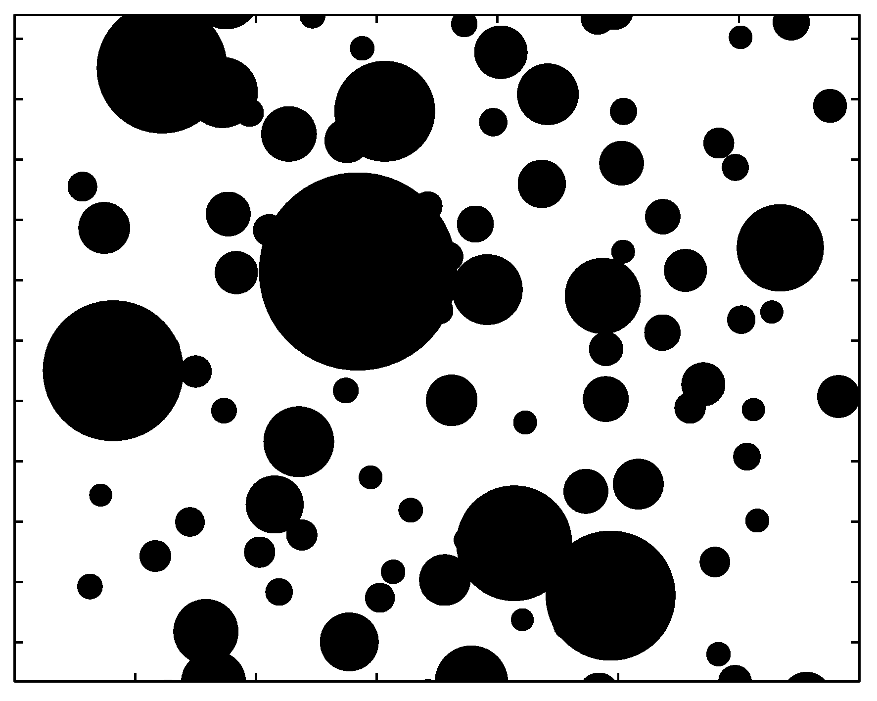
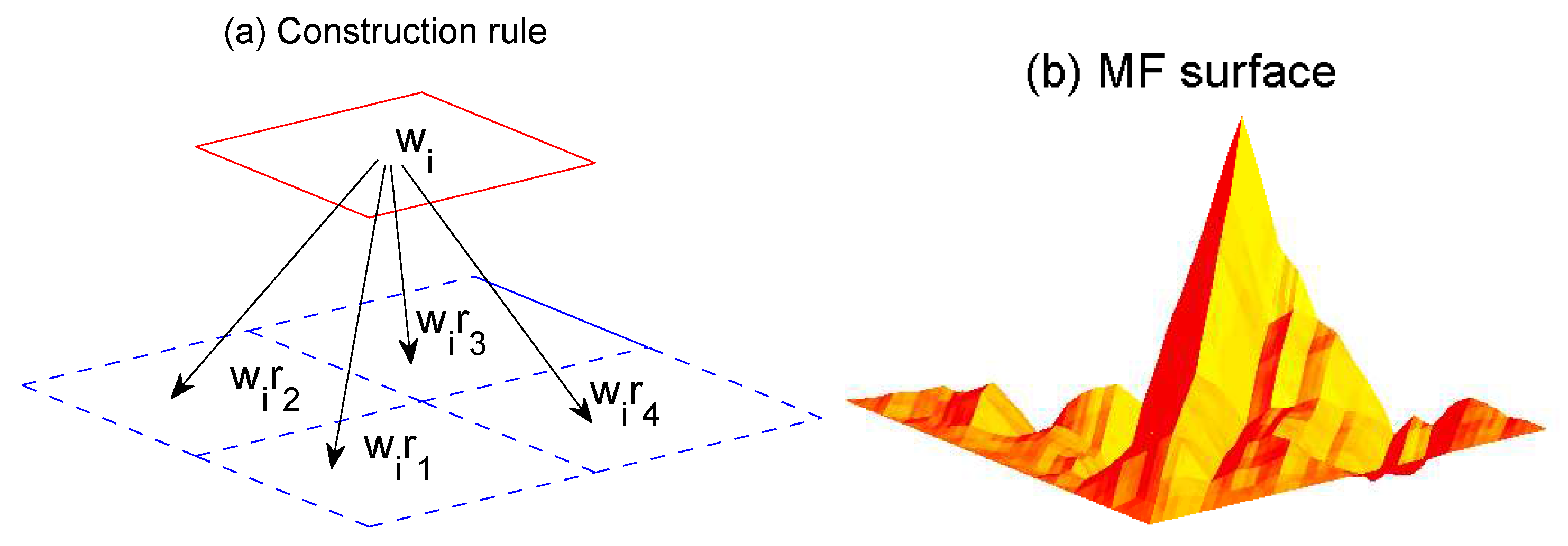
Two reasons make the power law extremely important in complexity science. One reason is that it embodies the notion of self-similarity, and thus is the natural mathematical tool for describing fractal phenomena. The other reason is that it often signifies great risk, due to infinite variance or even mean. To understand the first reason, imagine a large room with a lot of balls flying around. See Figure 2.

Assume the size of the balls follows a power law distribution,

$$p\left(r\right)\sim r^{-\alpha }.$$

(17)

When we observe the balls with our naked eyes, we normally will only pay more attention to the balls of certain size ranges—large balls will block our vision, and very small balls cannot be seen. Now assume that our eyes are comfortable with the scales $r_0$, $2r_0,r_0/2$, etc. Our perception is determined by the relevant abundance or the ratio of the balls of sizes $2r_0,r_0$, and $r_0/2$:

$$p\left(2r_0\right)/p\left(r_0\right)=p\left(r_0\right)/p(r_0/2)=2^{-\alpha }.$$

(18)

It is independent of $r_0$. Now suppose we view the balls through a microscope with a magnifying power of 100, so now our eyes will be focusing on the balls with scales $2r_0/100,r_0/100$, $r_0/200$, etc. The ratio of the balls on those scales will again be independent of the scale $r_0/100$. A perception independent of the scale is the essence of self-similarity.

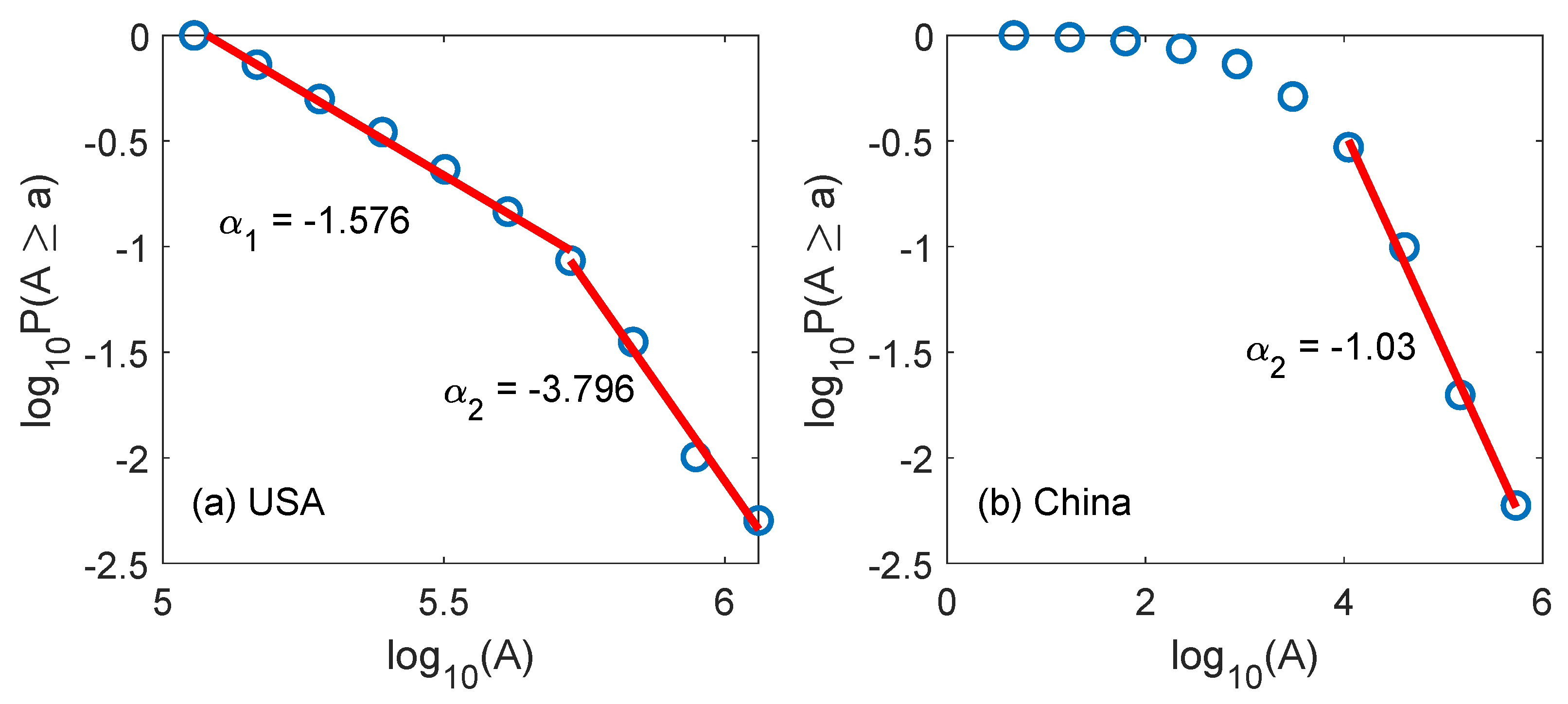
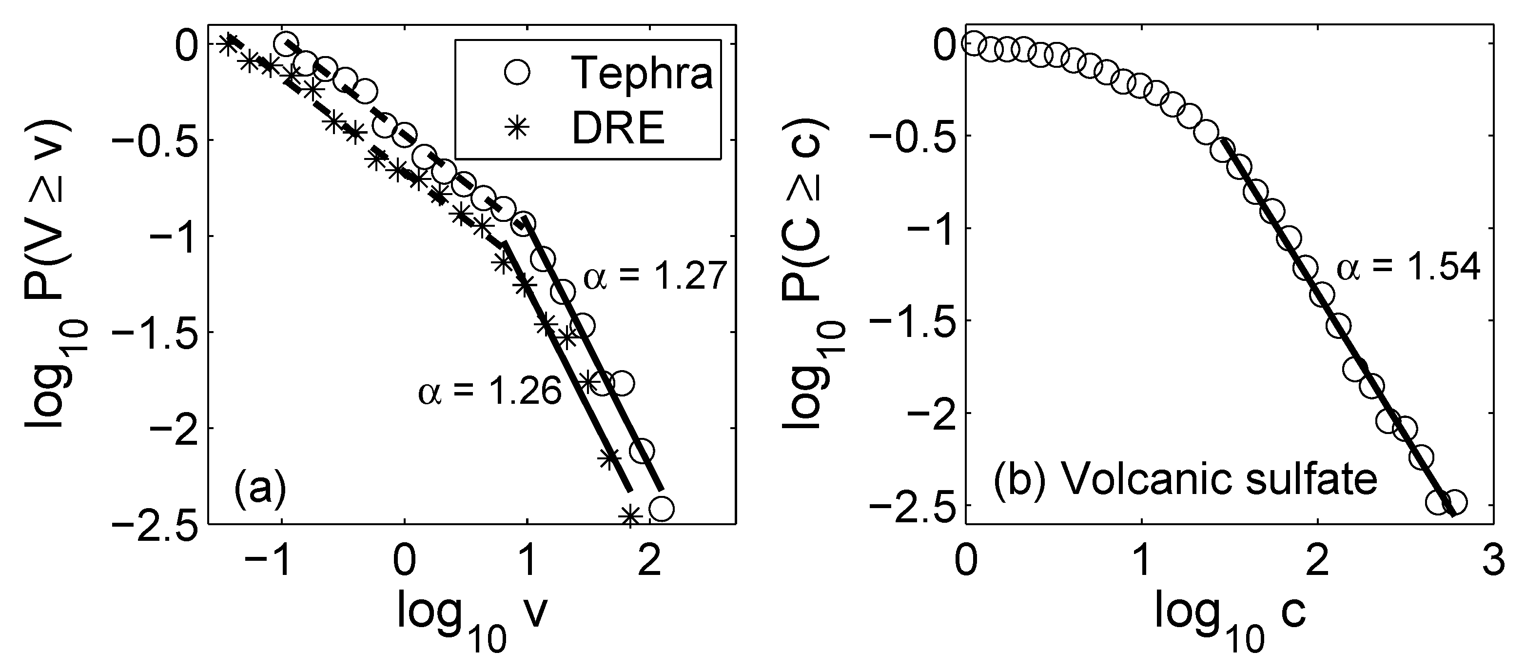
The second reason that the power law is associated with higher risks is easier to understand, since a power law distribution has infinite variance when $0<\alpha <2$ and even infinite mean when $0<\alpha \le 1$. Here, on one hand, one has to have some awe with the power law, as otherwise the cost could be tremendous. For example, during financial crises or economic downturns, the loss of the listed companies follows a power law distribution that is even heavier than the distribution of the gains of all profitable companies [51,52]. As further examples, the size of forest fires and volcanic eruptions also follow power law distributions (see Figure 3 and Figure 4), which has obvious implications for fire fighting or observation of volcanoes—going too close to the sites could easily lead to casualties. However, on the other hand, one also has to be mindful that having infinite variance or mean is not always associated with the severity of natural disasters. An important counterexample is flooding, as it has been found that stream flow of rivers in dry seasons (especially in desert areas) is better described by power law distributions, while that in wet seasons is better described by log-normal distributions [53]. In deserts, surely flooding does not constitute a major risk.

2.2.4. Mechanisms for Power Laws

The prevalence of power laws calls for development of models to explain the mechanism. Various models have been proposed, including Tsallis non-extensive statistics [55,56,57]. For a systematic discussion, we refer to Chapter 11 of [38]. Here, we note two of them, which appear to be relevant to many different scenarios and thus may better stimulate readers to readily find mechanisms when they find power laws from their data. One model is related to spatial heterogeneity and resource allocation (or availability). It is provided by the model that superposition of exponential distributions with different parameters can give rise to power law distributions. The other reflects the underlying local dynamics of the problem to some degree, and thus is in some sense more thought-provoking. The most well-known example of this class is perhaps the scale-free power law network model [58]. Another example is related to social segregation and crimes in a society: distributions of the ratio between sex offenders and the total population in the states of Ohio and New York in the USA follow power laws, as shown in Figure 5 [59]. While intuitively this must be driven by crimes (more concretely, sexual offenses) and instigated by laws preventing crimes, so far, however, a concrete model is still lacking. Such a model is surely worth developing in the future.

2.3. Essentials of Chaos Theory

Many readers can easily recall observing a sinusoidal signal with an oscilloscope. Assume we are examining some production line through monitoring of some signal. An aperiodic, highly irregular time series pops up. Is the signal simply some kind of noise? Very unlikely, since our system is deterministic. Can a seemingly random signal come from a deterministic system which can be described by only a few variables instead of a random system with infinite numbers of degrees of freedom? Yes, a chaotic system can do that! Not only so, many universal behaviors behind chaos have been uncovered. These findings have fundamental, far-reaching implications in science and engineering, and thus chaos theory, relativity, and quantum mechanics are considered the three most revolutionary scientific theories of the twentieth century.

To facilitate understanding of the essentials of chaos theory, in this section, we first explain the notion of phase space and transformation, then we present the basic properties of chaos. To satisfy curious minds, we will also give a flavor of analytical thinking. Finally, we explain how to reconstruct a proper phase space from a single variable (scalar time series) and estimate the few basic metrics (called invariants) that characterize a chaotic system.

2.3.1. Phase Space and Transformation

Phase space is the arena for the evolution of a dynamical system to unfold. It is spanned by all the variables needed to fully characterize the evolution of the system. To help one to better understand the idea, let us start from a system characterized by only two state variables, $X_1$ and $X_2$. Monitoring the system often amounts to examining the waveforms of $X_1\left(t\right)$ and $X_2\left(t\right)$. One may instead try to examine the trajectory defined by $(X_1\left(t\right),X_2\left(t\right))$, where t now is treated as an implicit parameter. The space spanned by $X_1$ and $X_2$ is the phase space (or state space) we are discussing. They could be position and velocity, for example. Employing phase space facilitates one to study the dynamics of a complicated system with a geometrical viewpoint. For some dynamical systems, irrespective of initial conditions, the trajectory eventually approaches a single point; this is called a globally stable fixed point solution. Of course, the situation could be more complicated. For example, the trajectory may converge to a closed loop, again irrespective of where the trajectory starts. This is called a globally stable limit cycle. The discrete counter part of a limit cycle is a periodic motion with certain period (say N): the corresponding attractor consists of N points, and the trajectory amounts to hopping among the N points with a definite order.

To be more familiar with the concept of phase space, it is useful to examine certain experience in daily life. To illustrate the idea, suppose we were going to a meeting by a taxi. On our way, there was a traffic jam, and the taxi got stuck. Afraid of being late, we decided to call the organizer. How would we describe our situation? Usually, we would tell the organizer where we got stuck and how quickly or slowly the taxi was moving. In other words, we actually have been using the concept of phase space as part of our daily language.

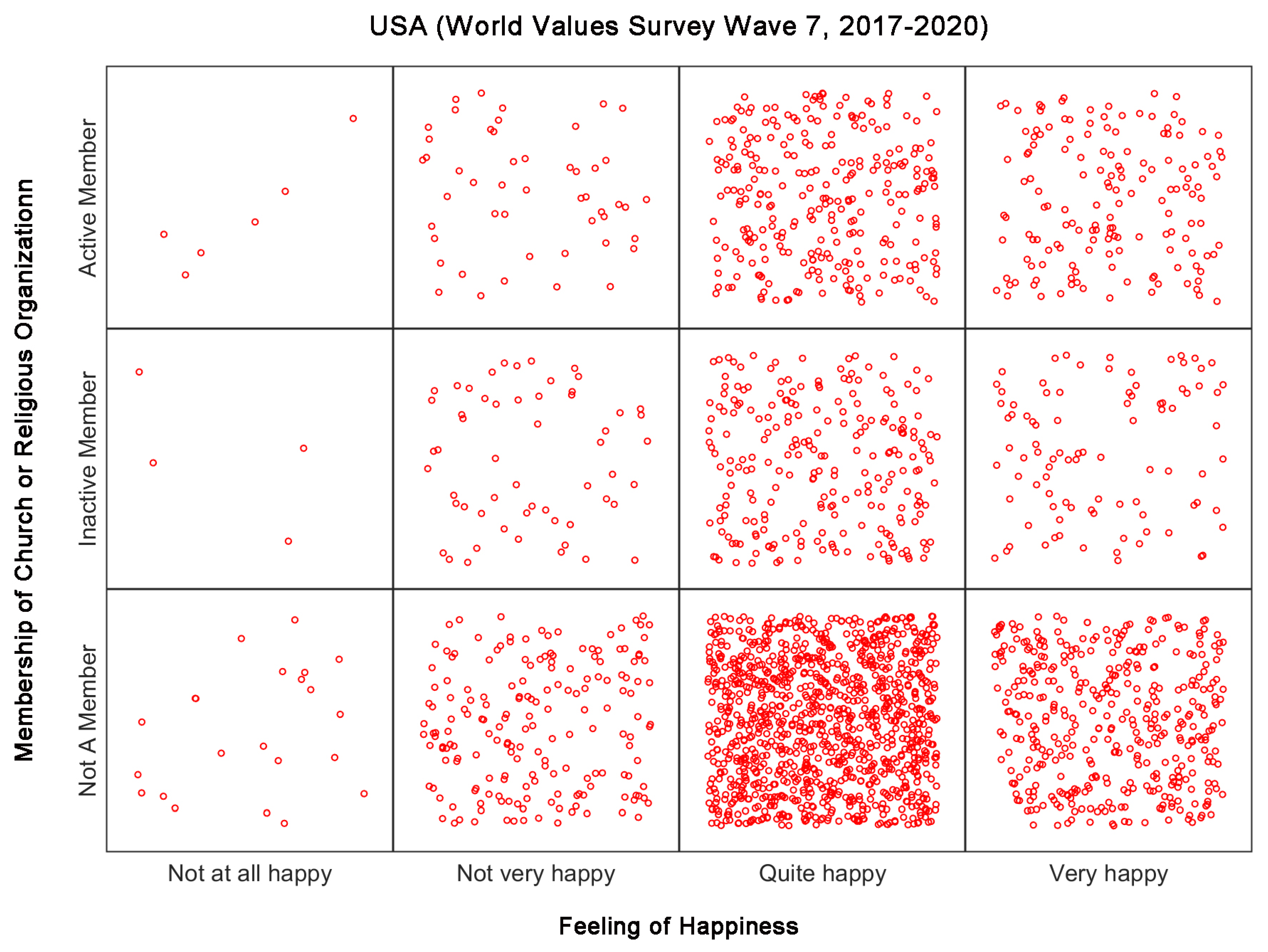
Although the concept of phase space is among the most basic in dynamical systems theory, its usefulness in geographical science has yet to be seriously explored [60]. To accelerate the coming of a time that phase space becomes as basic in geographical science as in complexity science, it is helpful to discuss two potential applications of phase space in geographical science. One application is top-down, that is, to systematically think about how many independent variables are needed to fully characterize an interesting and important problem in geographical science, and how each variable can be measured. The other application is bottom-up. It is easiest to illustrate the idea by using some variables in the World Value Survey (WVS, accessed on 17 April 2021, http://www.worldvaluessurvey.org/wvs.jsp) as an example. WVS is an interesting project that explores values and beliefs of people around the globe, how the values and beliefs evolve with time, and what social and political implications they may have. Since 1981, researchers have conducted representative national surveys in almost 100 countries. During the survey, a lot of variables have been deduced. We show here that phase space offers a convenient geometrical way to visualize the data and identify co-variations of the variables. For this purpose, we choose a variable that gives three levels of religious participation for people in the nations surveyed. The other variable we choose is happiness, which is given in four levels. How are the two variables related? How different are people in different countries in terms of these two variables? To gain insights into these interesting questions, we can form a phase space spanned by these two variables. The format of the survey data determines that people surveyed in a nation will belong to one of the 12 different categories. To fully utilize the notion of space, we can associate each category with a box. Instead of putting every person belonging to that category at one single point (e.g., the center of the box), we can generate two uniformly distributed random variables as the coordinate of the person in the corresponding box. Please see Figure 6. With such a visualization, one can immediately see the abundance of each category. When WVS data of different waves (times) are used, one can then examine variation of the percentage of people in each category over time for a nation, compare among different nations, deduce functional relationships between these two variables, and classify nations in the world into different clusters. Note Figure 6 may be called phase space ensemble based visualization, where an ensemble amounts to a participant in the survey.

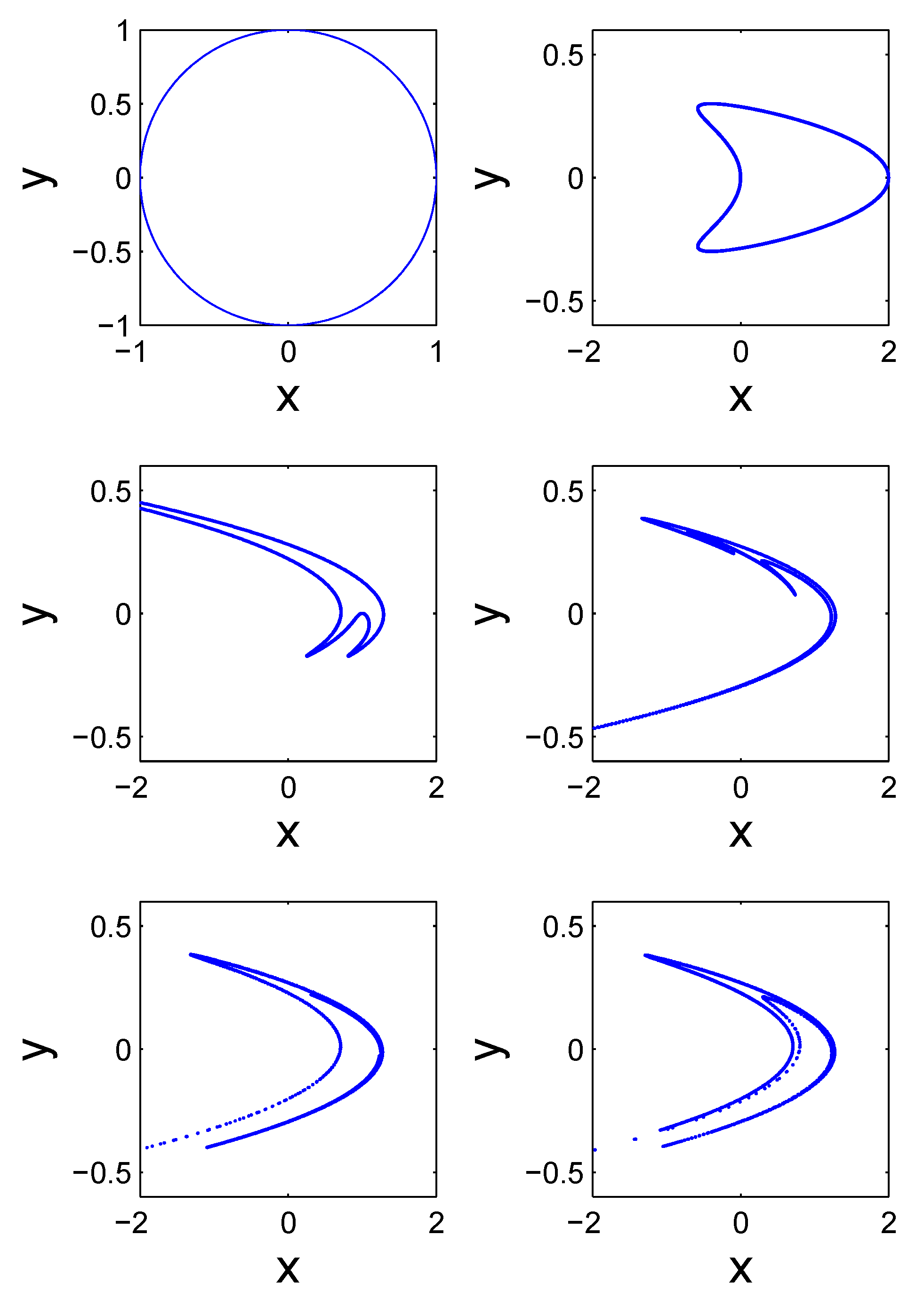
Next, let us consider transformations in phase space. A good way to grasp the idea is to imagine the following situation: on a very weedy day, a little boy went outside with a sheet of paper in his hand. He grabbed a handful of sand and put it on the paper. Then he released the paper in the air. How would the sand be swept across the sky? One could even think that originally the boy had arranged the sand to resemble the face of a person. How would the face be twisted by the wind? To make this discussion more concrete, we can consider how a unit circle is transformed by the Henon map [61]:

$$\begin{array}{ccc}\hfill x_{n+1}& =& 1-a{x}_n^2+y_n,\hfill \\ \hfill y_{n+1}& =& b{x}_n,\hfill \end{array}$$

(19)

where $a=1.4, b=0.3$. Figure 7 shows the successive (from left to right and top to bottom) images of the unit circle after $n=1,\cdots ,5$ iterations. Note that the fifth image is basically the Henon attractor one can find in textbooks, journal papers, or certain web sites. It is usually obtained by choosing an arbitrary initial condition and iterate the Henon map long enough. If the trajectory does not diverge, then after removing the transient points (which are the first few points here), the remaining trajectory (not connected by lines) will be very similar to the fifth image shown here. In our ensemble scenario, we observe that just after one iteration, the unit circle is already changed to a very different shape, and by the fourth iteration, the shape of the image is already very similar to the Henon attractor. By now, one could easily understand that the Henon attractor can either be readily obtained from an arbitrarily shaped phase space region (discarding initial conditions which lead to the divergence of the iterations) or by iterating a single arbitrary initial condition many times. The equivalence of the two approaches, one based on the evolution of ensembles in the phase space, the other based on long-time iterations, is a clear manifestation of the ergodic property of the Henon map (and more generally, chaotic systems).

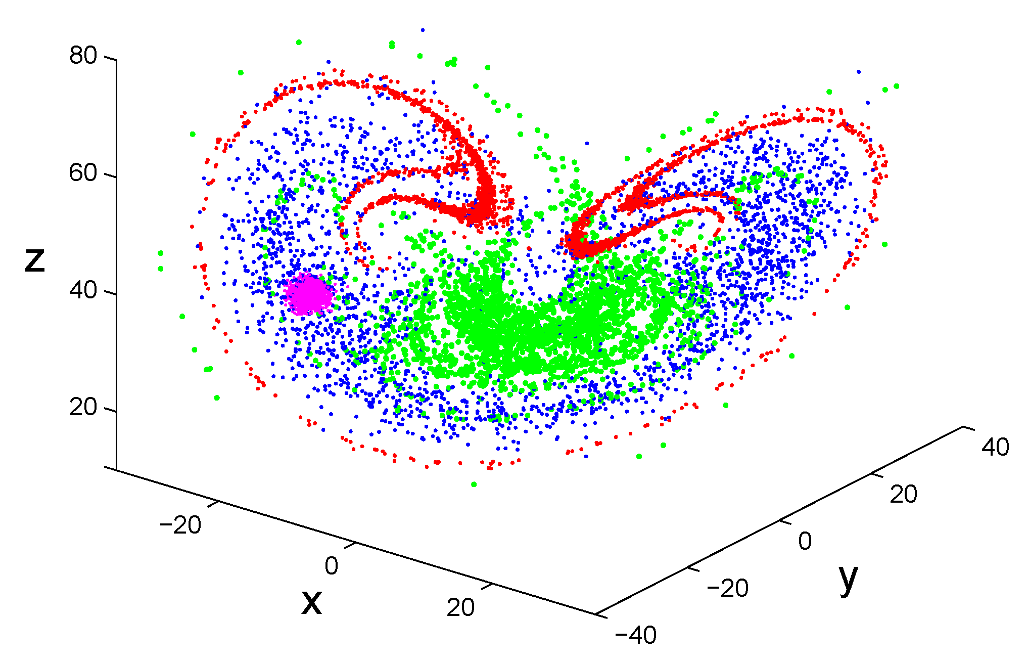
To enhance our understanding of the materials discussed so far, let us visually observe how chaos manifests itself in the chaotic Lorenz system:

$$\begin{array}{c}dx/dt=-16(x-y),\hfill \\ dy/dt=-xz+45.92x-y,\hfill \\ dz/dt=xy-4z.\hfill \end{array}$$

(20)

For this purpose, let us arbitrarily choose an initial condition, (−17.3432, −24.5966, 40.1096), perturb it 2500 times using standard Gaussian random variables with very small variance, and monitor the evolution of all those points. These initial conditions are shown in Figure 8 as a magenta block centered at our chosen initial condition. After 2 units of time, these initial conditions spread to the points labeled as red in the Figure. After another 2 units of time, the red points further evolve to the points labeled as green. Two more units of time later, the green points become the blue points. By that time, the shape of the points already resembles the chaotic Lorenz attractor we usually see in books, papers, and on the Internet.

2.3.2. Defining Properties of Chaotic Systems

The most important property of chaos is sensitive dependence on initial conditions. It means that a very small difference in the initial condition may lead to a completely different trajectory. To appreciate this property, one may imagine a butterfly flapping its wings sometime on a day in the Amazon rain forest. This contributes to a minor change in the global air currents. If the motion on that day is chaotic, then sunny weather in some city, say Ney York, could have been replaced by a rainy weather not long after the flapping of the butterfly’s wings. One may contrast this feature with a the traditional view, largely drawn from the study of linear systems, that small disturbances only produce proportional effects. Under the latter scenario, in order for the motion of the system to be random, the number of degrees of freedom has to be infinite.

Being the most important property of chaos, sensitive dependence on initial conditions has to be quantified. This is achieved by equating this property with an exponential divergence of nearby trajectories in the phase space. Let $d\left(0\right)$ be the small distance between two arbitrary trajectories at time 0, and let $d\left(t\right)$ be the distance between them at time t. Then, for true low-dimensional deterministic chaos, we have

$$d\left(t\right)\sim d\left(0\right)e^{{\lambda }_{1}t}$$

(21)

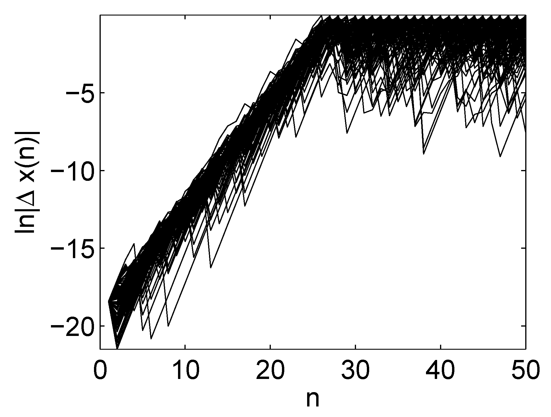
where ${\lambda }_1$ is called the largest positive Lyapunov exponent. This property of sensitive dependence on initial conditions of chaos can be conveniently illustrated by the chaotic Logistic map:

$$x_{n+1}=\mu x_n(1-x_n),$$

(22)

where $\mu =4$. We can generate, for example, 100 initial conditions by using uniformly distributed random numbers, and iterate the Logistic map to get 100 trajectories. We then perturb each of the initial conditions by a small error of ${10}^{-4}$ and regenerate the 100 trajectories. The evolution of the errors between the original and the perturbed trajectories is shown in Figure 9. Clearly we observe that the logarithm of the errors first increases with time linearly to about a time of $n=25$, then is saturated. Linear growth in a logarithmic scale amounts to exponential growth. By visual inspection, we can identify that ${\lambda }_1$ here is close to 0.7 (more precisely, $ln2$, which will be explained shortly). That errors very soon saturate is due to the fact that x defined by the logistic map is in the unit internal, as is the absolute value of the errors.

The largest positive Lyapunov exponent for the Henon map and the chaotic Lorenz system we discussed in Section 2.3.1 can also be conveniently computed based on time series data. This will be discussed shortly.

The trajectories of a chaotic attractor are bounded in the phase space. This is another fundamental property of the chaotic attractor. The ceaseless stretching due to exponential divergence of nearby trajectories, and folding from time to time due to boundedness of the attractor, make the chaotic attractor a fractal, characterized by

$$N\left(ϵ\right)\sim {ϵ}^{-D},ϵ\to 0,$$

(23)

where $N\left(ϵ\right)$ represents the (minimal) number of boxes, with linear length not larger than $ϵ$, needed to completely cover the attractor in the phase space. D is called the box-counting dimension of the attractor. Typically, it is a nonintegral number. For the chaotic Henon and Lorenz attractor, D is 1.2 and 2.05, respectively.

2.3.3. A Taste of Analysis

In order to better understand the key concept of chaotic dynamics, the sensitive dependence on initial conditions, let us engage in some analytic analysis. In practice, if one can identify from the problem a transformation similar to the following map, then one can be more than excited,

$$x_{n+1}=2x_n\mathrm{mod}1,$$

(24)

This is a map on the unit interval, where x is positive, and $\mathrm{mod}1$ means that only the fractional part of $2x_n$ is retained as $x_{n+1}$. The map can also be written as

$$x_{n+1}=\left\{\begin{array}{cc}2x_n,\hfill & 0\le x_n<1/2\hfill \\ 2x_n-1,\hfill & 1/2\le x_n<1,\hfill \end{array}\right.$$

(25)

This map in fact acts as a Bernoulli shift [62], or binary shift, since if we represent an initial condition $x_0$ in binary form

$$x_0=0.a_1{a}_2{a}_3\cdots =\sum _{j=1}^{\infty }{2}^{-j}{a}_j,$$

(26)

then

$$x_1=0.a_2{a}_3{a}_4\cdots ,$$

$$x_2=0.a_3{a}_4{a}_5\cdots ,$$

and so on, where each of the digits $a_j$ is either 1 or 0. Now it is clear that when $x_0$ is a rational number, the trajectory is periodic. In fact, we can easily find cycles of any length. For example, if $x_0$ is a 3-bit repeating sequence, such as $x_0=0.001001001\cdots$, then the trajectory is periodic with period 3. Since there are infinitely more irrational numbers than rational numbers in $[0,1)$, an arbitrary initial condition $x_0$ will be an irrational number with probability 1, and will almost surely generate an aperiodic, chaotic trajectory. Since after each iteration the map shifts one bit, a digit that is initially very unimportant, say the 80th digit (corresponding to $2^{-80}\approx {10}^{-24}$), becomes the first and the most important digit after 80 iterations. This is a vivid example that a small change in the initial condition makes a profound change in $x_n$. Clearly, the largest Lyapunov exponent ${\lambda }_1$ here is $ln2$.

Next, let us re-consider the logistic map with $\mu =4$. If we make a transformation,

$$x_n={sin}^2\left(2\pi y_n\right)$$

(27)

then the logistic map becomes the Bernoulli shift map discussed above. Therefore, the largest Lyapunov exponent ${\lambda }_1$ for the logistic map with $\mu =4$ is also $ln2$, as we already mentioned.

Now that we have gained some understanding by considering simple model systems, we can discuss how to characterize general chaotic systems. For a chaotic dynamical system with dimensions higher than 1, first we need to realize that exponential divergence can occur in more than one direction, and possibly in many directions. That means we have multiple positive Lyapunov exponents. We denote them by ${\lambda }^{+}$, among them, the largest one is usually denoted as ${\lambda }_1$. How are these Lyapunov exponents related to the rate of creation of new information, or in other words, loss of prior knowledge, in the system? To find the answer, we may partition the phase space into boxes of size $ϵ$, compute the probability $p_i$ that the trajectory visits box i, and finally calculate the Shannon entropy $I=-\sum p_{i}ln{p}_i$. For many systems, when $ϵ\to 0$, information increases with time linearly [63]

$$I(ϵ,t)=I_0+Kt$$

(28)

Here, $I_0$ is the initial entropy, and K is the celebrated Kolmogorov–Sinai (K-S) entropy [16,17]. Now let us consider the situation that all the initial conditions of the system are confined in a small region in the phase space. In this case, the initial probability in the chosen small region is 1, and 0 in all other regions. Therefore, $I_0=0$. For a chaotic system, because of the exponential divergence, the number of phase space regions visited by the system after a time of T is $N\propto e^{(\sum {\lambda }^{+})T}$, where ${\lambda }^{+}$ are the positive Lyapunov exponents we have already explained. If all these regions are visited by the trajectories with equal probability, then $p_i\left(T\right)\sim 1/N$, and the information function becomes

$$I\left(T\right)=-\sum _{i=1}^N{p}_i\left(T\right)ln{p}_i\left(T\right)=(\sum {\lambda }^{+})T$$

(29)

We thus have $K=\sum {\lambda }^{+}$. In general, if these phase space regions are not visited equally likely, then

$$K\le \sum {\lambda }^{+}$$

(30)

Grassberger and Procaccia suggest that equality usually holds [64].

2.3.4. Bifurcations, Routes to Chaos, and Universality

In practice, whenever one has a dynamical system model described by discrete maps or differential equations, then the first thing one needs to consider is if the model has a unique fixed point solution, and if yes, if the solution is locally or globally stable. If the model contains some controlling parameter(s), then one also has to consider if the qualitative feature of the solution changes with the parameter(s), and if yes, find out what kind of changes they are. One can also think if any features of the system are shared by systems in other fields. The last point is the universality issue. These considerations make it clear that studies of bifurcations, routes to chaos, and universality are of fundamental importance to the study of dynamical systems.

Fixed point solutions are one of the the limiting behaviors of dynamical systems. It turns out the limiting behaviors of dynamical systems are very rich. In order of increasing complexity, they are fixed points, limit cycles, torus, chaos, turbulence, and random motions [38]. Fixed points correspond to motions without any change; limit cycles correspond to periodic motions. We have already mentioned these two in the beginning of this section. Torus corresponds to quasi-periodic motions, i.e., the motion is characterized by two or more independent frequencies. Periodic and quasi-periodic motions may be associated with crystals and quasi-crystals, finding of the latter won Professor Daniel Shechtman a Nobel Prize in Chemistry in 2011. Fixed points, limit cycles, and torus all belong to regular motions.

Since chaotic and regular motions appear almost everywhere, we should ask if a chaotic motion may arise from a regular motion, and vice versa. Interestingly, the answer can be found by studying bifurcations and routes to chaos in dynamical systems. Here, it is critical to realize that the qualitative behaviors of the dynamics of a system may change when one or more controlling parameters are changed. The parameter values that cause such qualitative changes are called bifurcation points.

To better understand the notion of transitioning from one state to another, let us briefly consider the anti-globalization movement. As often reported in the media, anti-globalization activities are often accompanied with grandeur and truly praiseworthy ideals such as better democratic representation, advancement of human rights, fair trade, and sustainable development. However, this is only part of the story. The more fundamental cause of the anti-globalization movement is the flipping of power ranking among the participating countries—a country afraid of losing competitive edges or even being demoted to a lower position in the power ranking would attribute that to unfair trade, infringement of intellectual property rights, etc. While these concerns are not entirely unfounded, one has to realize that reward to countries participating in economic globalization cannot be linearly proportional to their ranking. As a result, rearrangement of the power ranking surely will occur. Here, the basic parameter controlling the transition from globalization to anti-globalization is associated with the rearrangement of the (relative) power ranking among the participating countries.

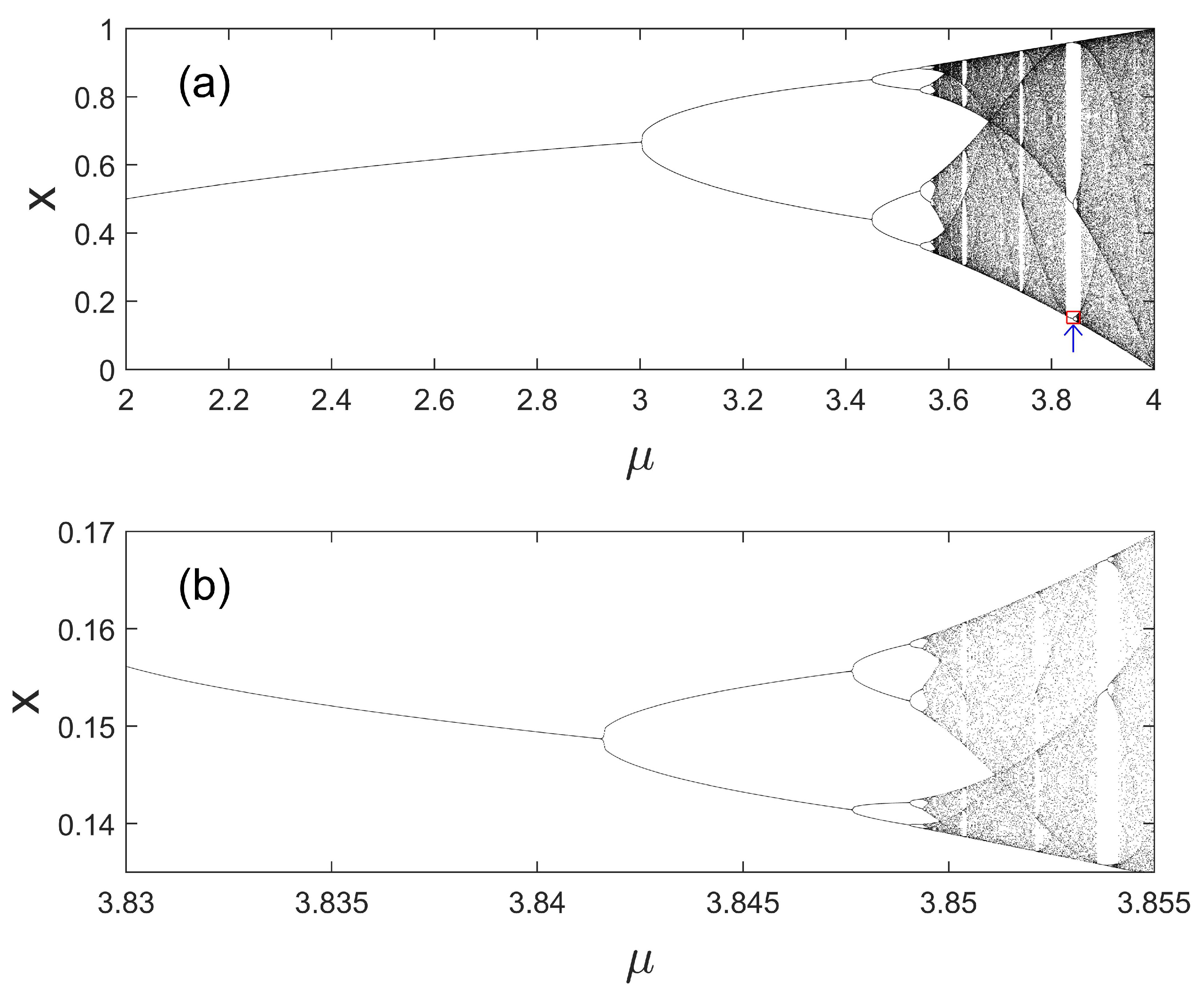
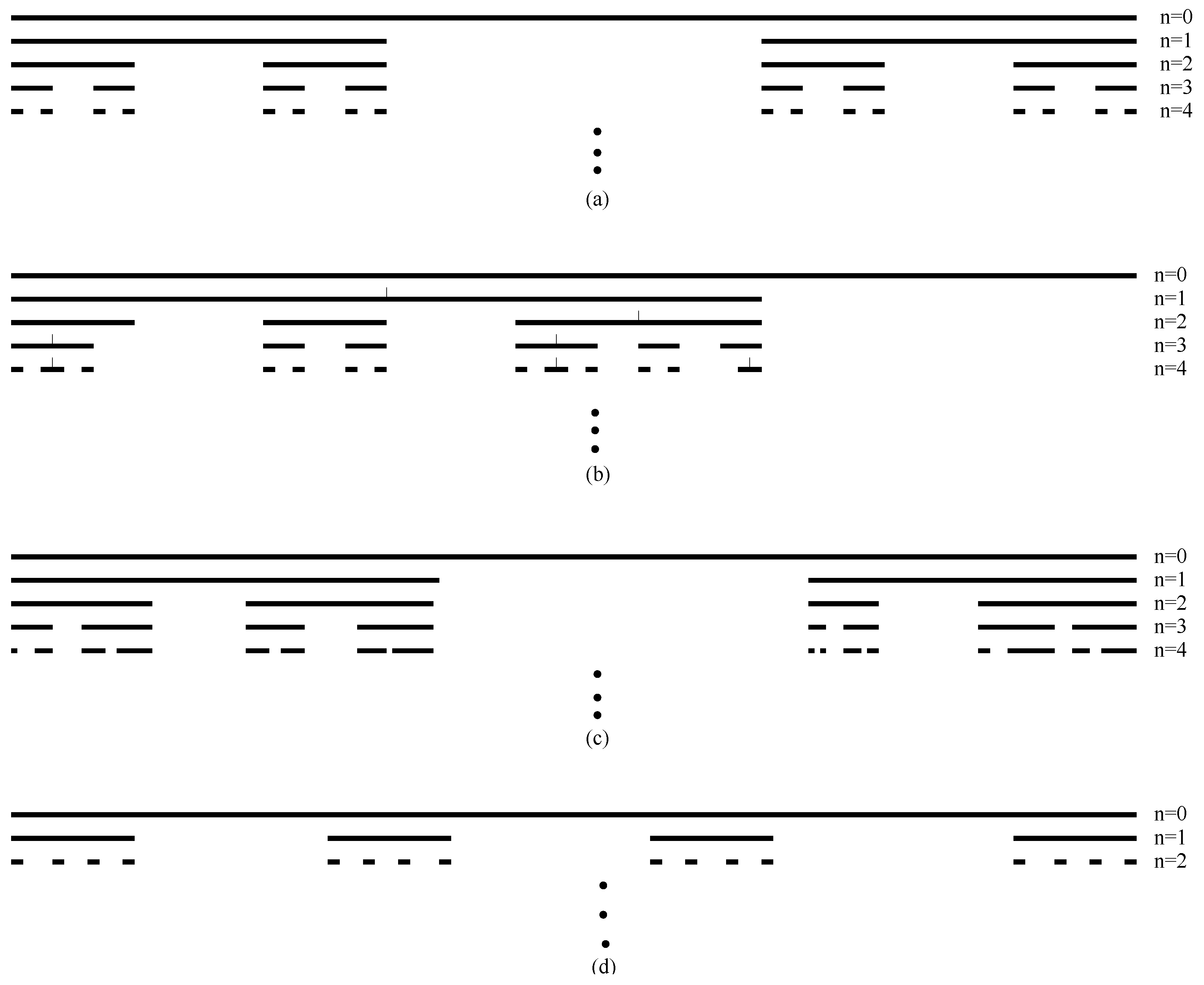
To understand bifurcations, let us analyze the logistic map described by Equation (22) again. Let us set $\mu =2$ and iterate the map starting with an initial condition $x_0=0.3$. With simple calculations, we can easily find that $x_n$ soon equals $0.5$ after a few iterations. If we choose $x_0=0.5$, then $x_1=x_2=\cdots =0.5$. This means that $0.5$ is a stable, fixed-point solution. While it is easy to prove this statement rigorously [38], here, let us resort to simulations: For any $\mu$, where $\mu \in [2,4]$, we choose an arbitrary initial value of $x_0$, and iterate Equation (22). After discarding the initial iterations so that the solution of the map has stabilized, we retain a large number (say, 100) of the value of the iterations, and form a scatter plot of those values with $\mu$. When the map has a globally attracting fixed-point solution, then the recorded values of $x_n$ will all become the same since the transients have been discarded. In this situation, one only observes a single point with the horizontal axis being the chosen $\mu$ and the vertical axis being the converged value of $x_n$. For a periodic solution with period m, one can observe m distinct points on the vertical axis. When the motion becomes chaotic, one observes on the vertical axis as many distinct points as one records (100 in our example). Figure 10a shows the bifurcation diagram for the logistic map—the interesting structure is the celebrated period-doubling bifurcation to chaos.

Figure 10a embodies more structures than one could comprehend by a simple glance. For example, if one enlarges Figure 10a the small rectangular region containing the period-3 window, then one obtains Figure 10b. We have again observed a period-doubling route to chaos! (To truly understanding the presentations here, it is beneficial for readers new to chaos theory to write a simple program to reproduce Figure 10a,b).

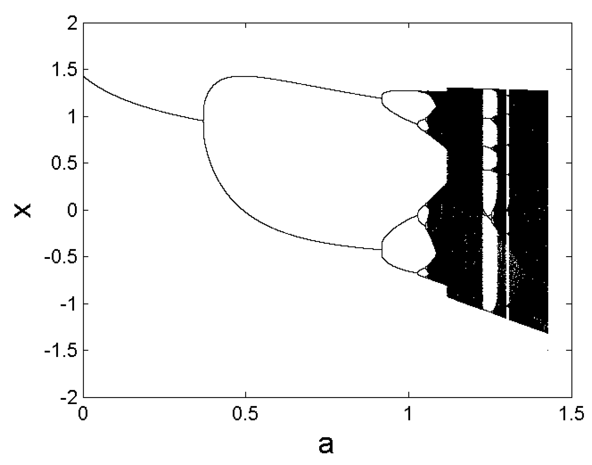
Having been observed in many diverse fields, period-doubling bifurcation to chaos is one of the most studied and most celebrated routes to chaos [65]. To better comprehend this universality, it is worth noting that it also underlies the bifurcations in the Henon map (see Figure 11) and the Lorenz system. In fact, the notion of universality can be quantified for the period-doubling bifurcation to chaos, through the Feigenbaum constant defined by

$$\delta =\underset{k\to \infty }{lim}\frac{{\mu }_k-{\mu }_{k-1}}{{\mu }_{k+1}-{\mu }_k}=4.669201\cdots .$$

(31)

Other routes to chaos also exist. They include the well-known quasi-periodicity route [66] and the intermittency route [67]. The former refers to when a controlling parameter is changed, the motion of the system changes from a periodic motion with one basic frequency, a quasi-periodic motion with two or more basic frequencies, to chaotic motions. This route has been observed in many mechanical and physical systems, including fluid systems. A bit surprisingly, this route has also manifested itself in the Internet transport dynamics (concretely, a variable amounting to the round-trip time of a message transmitting through the Internet can change from periodic and quasi-periodic motion to chaos when the congestion level increases [68]). The third classic route to chaos, intermittency, refers to the behavior that the motion of the system alters between smooth and chaotic modes, again when a controlling parameter is changed. This route to chaos is very relevant to many nonstationary phenomena in nature, including river flow dynamics, which are very different in wet and dry seasons.

2.3.5. Chaotic Time Series Analysis

In this big data era, data of all kinds, including time series data, have been accumulating explosively. Many techniques developed in the context of chaotic time series analysis will be of tremendous value for the analysis of all kinds of complex time series data whenever linear approaches are not sufficient. Below, we explain briefly but systematically all the main components of chaotic time series analysis.

A. 

Optimal embedding

Often, a complicated dynamical system described by $d\overrightarrow{U}/dt=f(\overrightarrow{U})$ lives in a high-dimensional phase space, where $\overrightarrow{U}$ is a vector. In many situations, we may only be able to access a single variable, say x, instead of many components of $\overrightarrow{U}$. In the simplest case, x is just a component of $\overrightarrow{U}$, say $U_1$. In general, x may be a function of $\overrightarrow{U}$. From $x\left(t\right)$, how much can we deduce the behavior of the dynamical system? The answer is a lot can be learned from x, thanks to the Takens embedding theorem. The basic procedure is to construct vectors according to the following equation [69,70,71],

$$V_i=[x\left(i\right),x(i+L),\dots ,x(i+(m-1)L)],$$

(32)

where m is the embedding dimension and L the delay time. More explicitly, we have

$$\begin{array}{c}\hfill V_1=[x\left(t_1\right),x(t_1+\tau ),x(t_1+2\tau ),\dots ,x(t_1+(m-1)\tau ],\\ \hfill V_2=[x\left(t_2\right),x(t_2+\tau ),x(t_2+2\tau ),\dots ,x(t_2+(m-1)\tau ],\\ \hfill ⋮\\ \hfill V_j=[x\left(t_j\right),x(t_j+\tau ),x(t_j+2\tau ),\dots ,x(t_j+(m-1)\tau ],\\ \hfill ⋮\end{array}$$

(33)

where $t_{i+1}-t_i=\Delta t$ and $\tau =L\Delta t$. We thus obtain a discrete dynamical system (i.e., a map),

$$V_{n+1}=M\left(V_n\right).$$

(34)

If the original dynamical system has an attractor with a boxing counting dimension D defined by Equation (23), then so long as $m>2D$, topologically the dynamics of the original system described by $d\overrightarrow{U}/dt=f(\overrightarrow{U})$ are equivalent to that described by Equation (34). In this case, the procedure using the delay coordinates is called an embedding. In proving this theorem, two properties of differential equations play key roles: (1) for any initial condition, a set of ODEs has a unique solution, and this ensures that trajectories corresponding to different initial conditions in the phase space do not intersect in the phase space; (2) a trajectory corresponding to a specific initial condition does not self-intersect in the phase space; when m is sufficiently large, self-intersection will be fully eliminated.

In practical applications, m and L have to be determined according to some optimization procedure. To appreciate the issue, let us consider the harmonic oscillator described below, which is among the simplest dynamical systems:

$$\frac{d^{2}x}{d{t}^2}=-\omega x.$$

(35)

Of course, we can also write it as

$$\frac{dx}{dt}=y,\frac{dy}{dt}=-\omega x,$$

(36)

The general solution is

$$x\left(t\right)=Acos(\omega t+{\varphi }_0),y\left(t\right)=Asin(\omega t+{\varphi }_0).$$

(37)

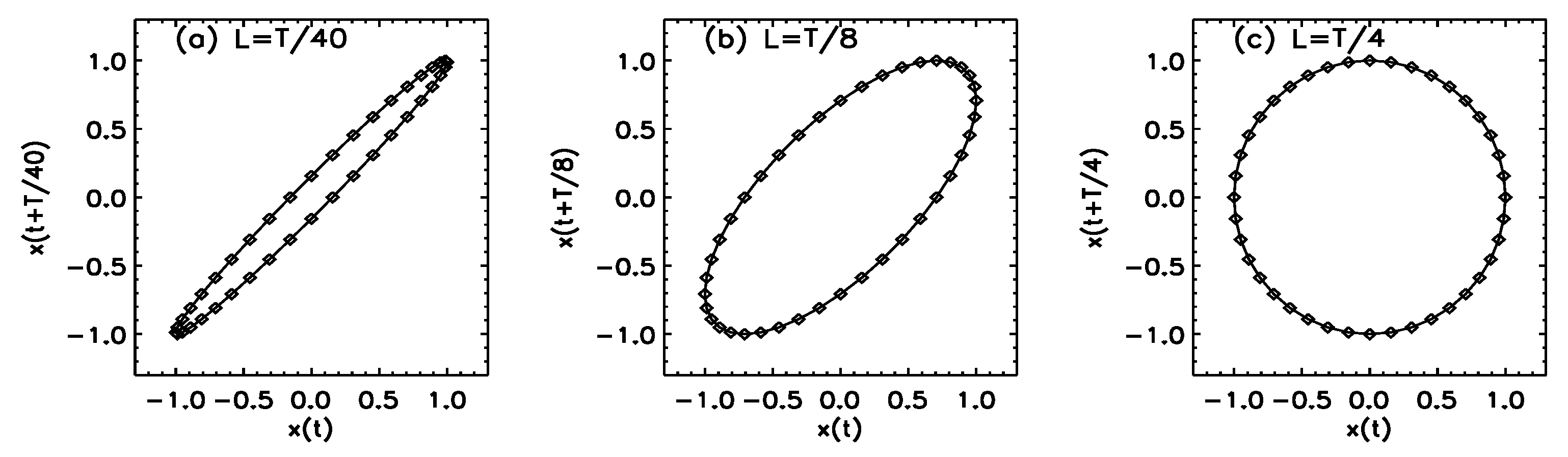
Here, the phase space is a 2D plane with coordinates x and y. Now consider the case that we can only measure $x\left(t\right)$. Using the embedding procedure with $m=2$, we obtain $V\left(t\right)=\left[x\right(t),x(t+\tau \left)\right]$. Figure 12 shows embeddings with $\tau =T/40,T/8,T/4$, where $T=2\pi /\omega$ is the period of the oscillation. When $\tau =T/4$, the difference between the two components, $x\left(t\right)$ and $x(t+\tau )$, in terms of angle is $\pi /2$. With this angle difference, the cosine function becomes the sine function. That is, $x(t+\tau )$ becomes $y\left(t\right)$). Therefore, the reconstructed dynamical system is the same as the original one. In this simple example, the minimal embedding dimension m is 2, and the optimal delay time L is 1/4 of the period. The consequence of using this optimal delay time is that the motion in the reconstructed phase plane is the most uniform—the phase velocity is the same everywhere in the case of Figure 12c, but not in those of Figure 12a,b.

Since the 1980s, a number of excellent methods have been proposed to optimally determine m and $\tau$. Below we describe two approaches, which have been extensively tested and are very systematic.

(1) 

False nearest-neighbor method: This is a geometrical method. Consider the situation in which an $m_0$-dimensional delay reconstruction is embedded but an $(m_0-1)$-dimensional reconstruction is not. Passing from $m_0-1$ to $m_0$, self-intersection in the reconstructed trajectory is eliminated. This feature can be quantified by the sharp decrease in the number of nearest neighbors when m is increased from $m_0-1$ to $m_0$. Therefore, the optimal value of m is $m_0$. More precisely, for each reconstructed vector $V_i^{\left(m\right)}=[x\left(t_i\right),x(t_i+\tau ),x(t_i+2\tau ),\cdots ,x(t_i+(m-1)\tau )]$, its nearest neighbor $V_j^{\left(m\right)}$ is found (to ensure unambiguity, here the superscript $\left(m\right)$ is used to emphasize that this is an m-dimensional reconstruction). If m is not large enough, then $V_j^{\left(m\right)}$ may be a false neighbor of $V_i^{\left(m\right)}$ (something like both the north and south poles are mapped to the center of the equator, or multiple different objects have the same shadow). If embedding can be achieved by increasing m by 1, then the embedding vectors become $V_i^{(m+1)}=[x\left(t_i\right),x(t_i+\tau ),x(t_i+2\tau ),\cdots ,x(t_i+(m-1)\tau ,x(t_i+m\tau )]=[V_i^{\left(m\right)},x(t_i+m\tau )]$ and $V_j^{(m+1)}=[V_j^{\left(m\right)},x(t_j+m\tau )]$, and they will no longer be close neighbors. Instead, they will be far apart. The criterion for optimal embedding is then

$$R_f=\frac{|x(t_i+m\tau )-x(t_j+m\tau )|}{\left|\right|V_i^{\left(m\right)}-V_j^{\left(m\right)}\left|\right|}>R_T,$$

(38)

where $R_T$ is a heuristic threshold value. Abarbanel [72] recommends $R_T=15$.

After m is determined, $\tau$ can be obtained by minimizing $R_f$.

While this method is intuitively appealing, it should be pointed out that it works less effectively in the noisy case. Partly, this is because nearest neighbors may not be well defined when data have noise.

(2) 

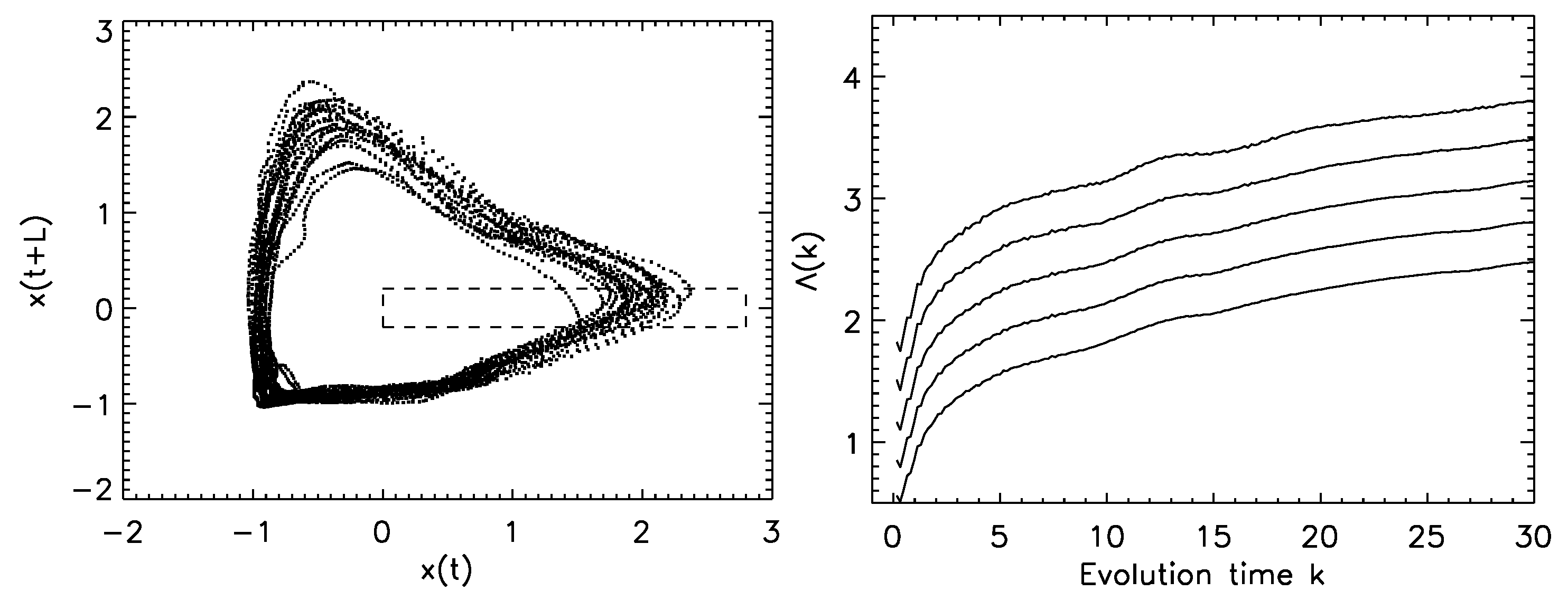
Time-dependent exponent curves: This is a dynamical method developed by Gao and Zheng [73,74]. The basic idea is that false neighbors will fly apart rapidly if we follow them on the trajectory. Denote the reconstructed trajectory by $V_1^{\left(m\right)},V_2^{\left(m\right)},\cdots$. If $V_i^{\left(m\right)}$ and $V_j^{\left(m\right)}$ are false neighbors, then it is unlikely that points $V_{i+k}^{\left(m\right)},V_{j+k}^{\left(m\right)}$, where k is the evolution time, will remain close neighbors. That is, the distance between $V_{i+k}^{\left(m\right)}$ and $V_{j+k}^{\left(m\right)}$ will be much larger than that between $V_i^{\left(m\right)}$ and $V_j^{\left(m\right)}$ if the delay reconstruction is not an embedding. The metric recommended by Gao and Zheng is

$$\Lambda (m,L,k)=〈ln\left(\frac{\parallel V_{i+k}-V_{j+k}\parallel }{\parallel V_i-V_j\parallel }\right)〉.$$

(39)

Here, for simplicity, the superscript $\left(m\right)$ in the reconstructed vectors is no longer indicated. The angle brackets denote the average of all possible $(V_i,V_j)$ pairs satisfying the condition

$${ϵ}_i\le \parallel V_i-V_j\parallel \le {ϵ}_i+\Delta {ϵ}_i,i=1,2,3,\cdots ,$$

(40)

where ${ϵ}_i$ and $\Delta {ϵ}_i$ are more or less arbitrarily chosen small distances. Geometrically speaking, Equation (40) defines a shell, with ${ϵ}_i$ being the diameter of the shell and $\Delta {ϵ}_i$ the thickness of the shell. When ${ϵ}_k=0$, the shell becomes a ball; in particular, if the embedding dimension m is 2, then the ball is a circle. Note that the computation is carried out for a series of shells, $i=1,2,3,\cdots$, and $\Delta {ϵ}_i$ may depend on the index i. With this approach, the effect of noise can be greatly suppressed.

As a rule of thumb, Gao and Zheng find that for a fixed small k, the minimal m is such that when further increasing m, $\Lambda (m,L,k)$ no longer decreases significantly. After m is determined, L can be chosen by minimizing $\Lambda (m,L,k)$.

Now that we have determined an optimal embedding, we can discuss how to estimate the largest positive Lyapunov exponent, dimension, and Kolmogorov entropy of chaotic attractors.

B. 

Estimation of the largest positive Lyapunov exponent

A number of algorithms for estimating the Lyapunov exponents have been developed. A classic method is Wolf et al.’s algorithm [75]. The basic idea is to select a fiducial trajectory and monitor how the deviation from it grows with time. Let the distance between the two trajectories at time $t_i$ and $t_{i+1}$ be $d_i^{\prime }$ and $d_{i+1}$. The rate of the exponential divergence over this time period is given by

$$\frac{ln(d_{i+1}/d_i^{\prime })}{t_{i+1}-t_i}.$$

To ensure exponential divergence, the distance between the two trajectories has to be always small. Therefore, when $d_{i+1}$ exceeds a certain chosen threshold value, something has to be done: a new point in the direction of the vector of $d_{i+1}$ is used so that $d_{i+1}^{\prime }$ is very small compared to the size of the attractor. This procedure is called normalization. After n repetitions of the procedure, we obtain

$${\lambda }_1=\sum _{i=1}^{n-1}\left[\frac{t_{i+1}-t_i}{{\sum }_{i=1}^{n-1}(t_{i+1}-t_i)}\right]\left[\frac{ln(d_{i+1}/d_i^{\prime })}{t_{i+1}-t_i}\right]=\frac{{\sum }_{i=1}^{n-1}ln(d_{i+1}/d_i^{\prime })}{t_n-t_1}.$$

(41)

Note the normalization procedure is where the novelty of the algorithm lies. The necessity of this step can be best understood by resorting to Figure 9: The computation from $t_i$ to $t_{i+1}$ amounts to one curve in Figure 9—when error saturates, a new round of computation has to begin; renormalization along the direction of the latest vector ensures that the evaluation of the largest positive Lyapunov exponent is along the most unstable dynamics of the data. This is especially important for high-dimensional cases, where there are multiple unstable directions (and therefore multiple positive Lyapunov exponents).

Unfortunately, the Wolf’s algorithm suffers from two serious problems. One is that it does not and cannot tell how to determine a threshold value suitable for the normalization procedure. The other is even more serious: it assumes but does not test exponential divergence. As a consequence of the second problem, a positive ${\lambda }_1$ could arise from any type of noisy data, including independent identically distributed (IID) random variables, as long as all the distances used in the computation are small. Therefore, the approach can often interpret a noisy process as a chaotic motion. To see why this is so, consider the case that $d_i^{\prime }$ is small. At the next time, $d_{i+1}$ usually will be larger than $d_i^{\prime }$. This may be called that evolution would move $d_i^{\prime }$ to the most probable spacing. In the case of fully random sequence and without embedding, this “evolution” will be completed in just one time step; when embedding is used, embedding vectors automatically incorporate correlations, and this “evolution” will be completed in m time steps, where m is the embedding dimension. In both situations, $d_{i+1}$, being in the middle step evolving from $d_i^{\prime }$, typically will be larger than $d_i^{\prime }$; consequently, a quantity computed using Equation (41) will be positive.

While a positive ${\lambda }_1$ is more likely to be produced by Wolf’s algorithm, it should also be noted that certain implementations of the algorithm, such as that based on neural networks, may have to choose an initial spacing of $d_i^{\prime }$ larger than the most probable spacing, so that the computation can return a nonempty result—this is more so when noise is stronger. In that case, ${\lambda }_1$ estimated will be negative, enticing one to interpret the data under investigation to be non-chaotic when the data contain more noise. Of course, this interpretation is also incorrect since, in principle, entropy for noisy systems is infinite, but not negative (for more details on this issue, we refer to [76]).

To overcome the problems with Wolf’s algorithm, a number of methods have been proposed. One algorithm is independently developed by Rosenstein et al. [77] and Kantz [78]. Another algorithm is developed by Gao and Zheng [73,74,79], published at about the same time. We first describe the former.

With the method of Rosenstein et al. [77] and Kantz [78], one first chooses a reference point and finds its $ϵ$-neighbors $V_j$. One then follows the evolution of all these points and computes an average distance after a certain time. Finally, one chooses many reference points and takes another average. Following the notation of Equation (39), these steps can be described by

$$\Lambda \left(k\right)={〈ln{〈\parallel V_{i+k}-V_{j+k}\parallel 〉}_{averageoverj}〉}_{averageoveri},$$

(42)

where $V_i$ is a reference point and $V_j$ are neighbors to $V_i$, satisfying the condition $\parallel V_i-V_j\parallel <ϵ$. If $\Lambda \left(k\right)\sim k$ for a certain intermediate range of k, then the slope is the largest Lyapunov exponent. This is the most fundamental part of the algorithm: it explicitly tests whether the dynamics of the data possess exponential divergence or not.

While in principle this method can distinguish chaos from noise, with finite noisy data it may not function as desired. One of the major reasons is that in order for the $averageoverj$ to be well defined, $ϵ$ has to be small. In fact, sometimes the $ϵ$-neighborhood of $V_i$ is replaced by the nearest neighbor of $V_i$. For this reason, the method cannot handle short, noisy time series well.

Gao and Zheng’s algorithm [73,74,79] contains three basic ingredients: Equations (39) and (40), and the condition

$$|i-j|>w.$$

(43)

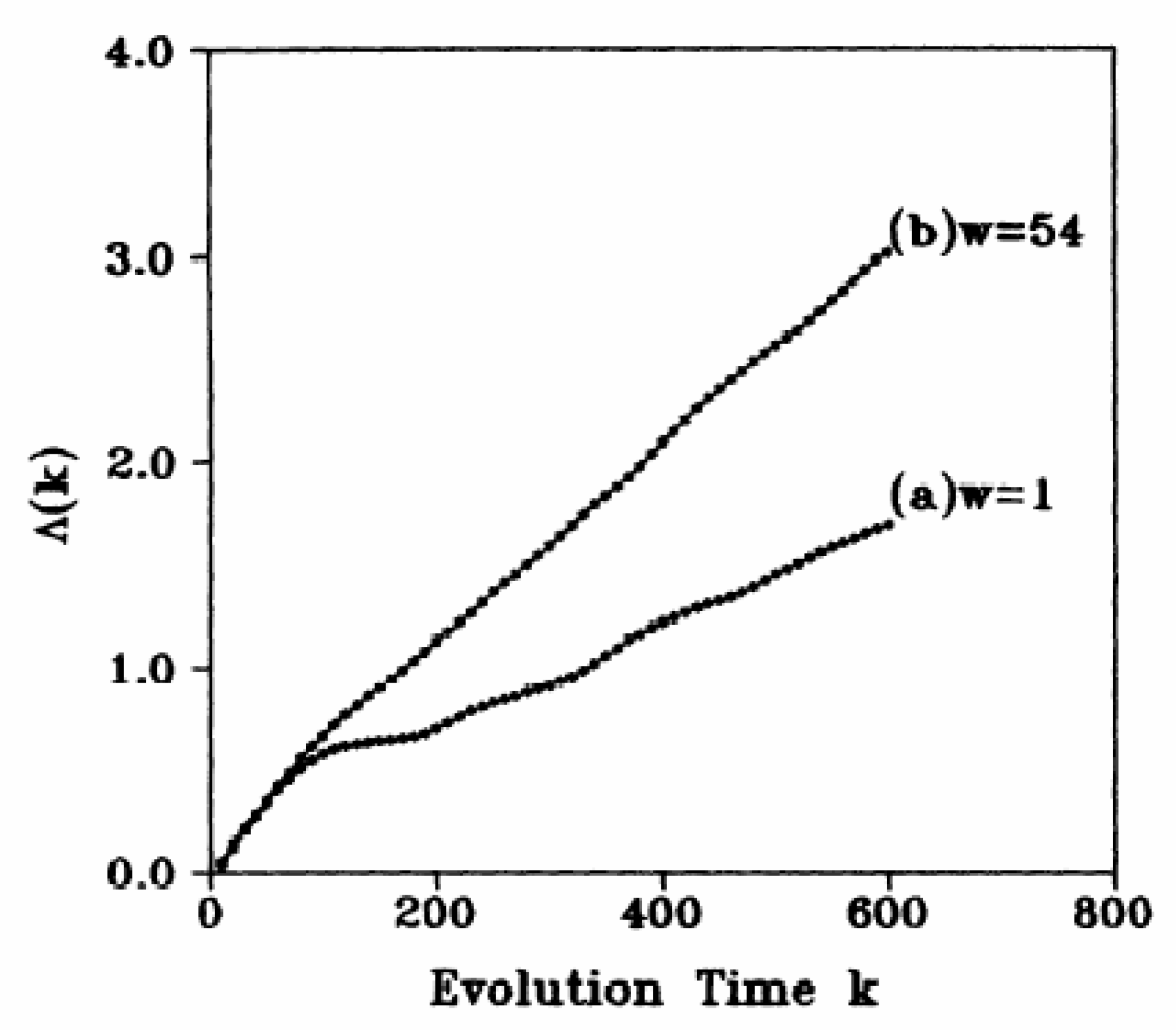
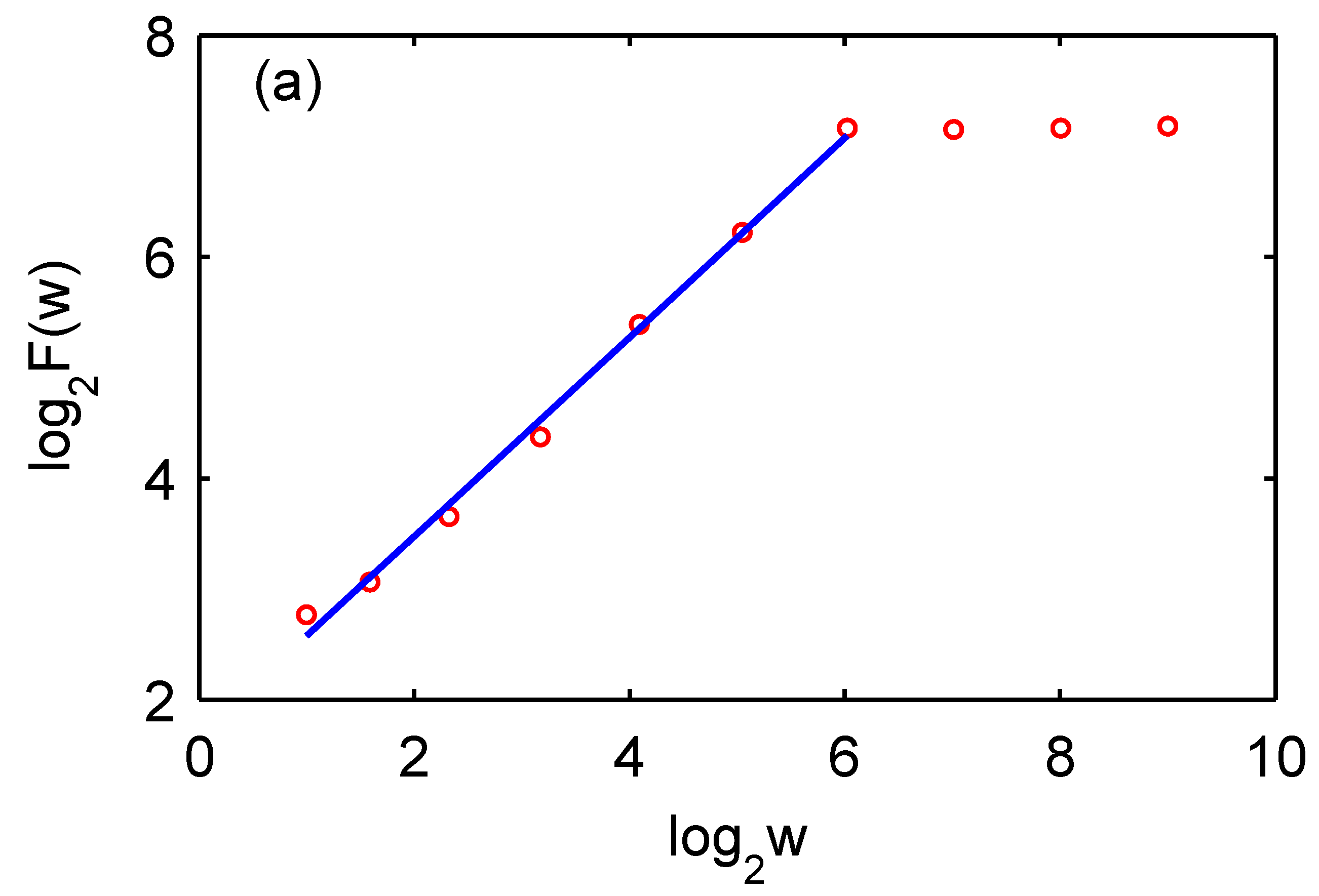
Equation (39) plays the same role as but is simpler than Equation (42), since it eliminates the necessity of performing two rounds of averages. More important are the conditions specified by two Inequalities (40) and (43). The condition specifying the series of shells makes the method a direct test for deterministic chaos, which will be explained momentarily. The condition specified by Inequality (43) ensures that tangential motions corresponding to the condition that $V_i$ and $V_j$ follow each other along the orbit are removed. Tangential motions contribute a Lyapunov exponent of zero and, hence, severely underestimate the positive Lyapunov exponent. An example is exhibited in Figure 13. We find that when $w=1$, the slope of the curve severely underestimates the largest positive Lyapunov exponent, while $w=54$ solves the problem. In practice, w can be chosen to be larger than one orbital time, when orbital times are defined in the dynamical system (Lorenz and Rossler attractor are such systems). If an orbital time cannot be defined, it can be more or less arbitrarily set to be a large integer if the dataset is not too small.

To see how the condition specifying the series of shells gives rise to a direct test for deterministic chaos, we can compare the behavior of the time-dependent exponent curves for truly chaotic data and independent, identically distributed random variables. The basic results are illustrated in Figure 14. We observe that for true chaotic signals, the time-dependent exponent curves from different shells not only grow linearly for some intermediate range of the evolution time k, but form a common envelope. As one expects, the slope of the common envelope gives an accurate estimation of the largest positive Lyapunov exponent. Such a common envelope does not exist for IID random variables. In fact, the behavior of the IID random variables vividly illustrates the problems with Wolf’s algorithm: $\Lambda \left(k\right)/k\delta t$ amounts to the largest positive Lyapunov exponent; the very fact that it critically depends on k and the size of the shells is a clear manifestation that the data under study are random.

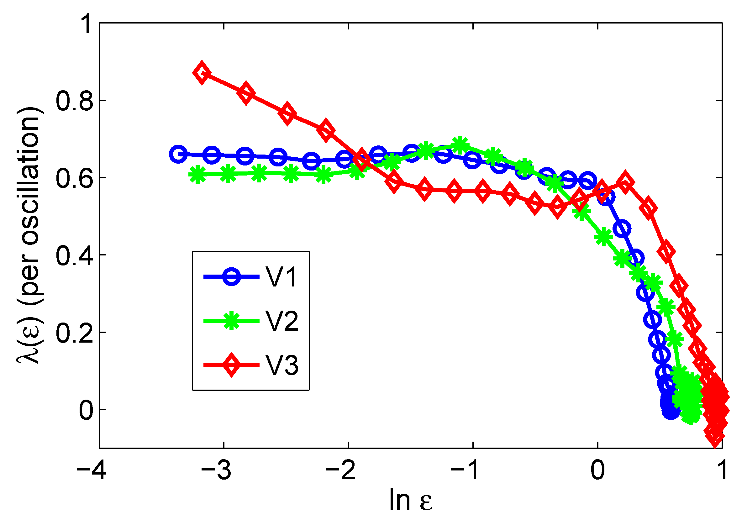
As one can anticipate, when a chaotic signal is contaminated by noise, the common envelope will gradually disappear with an increasing amount of noise. In general, this is true for both measurement noise and dynamical noise, where measurement noise is the noise superimposed onto a signal during a measurement process, while dynamical noise is a noise that actively participates in the dynamics of the system (i.e., appears in the basic equation(s) of the dynamical system). When a system dynamic is oscillatory and characterized by a limit cycle, with dynamical noise, in certain situations, a stochastic oscillator will arise, with the frequency of the oscillation still close to that of the original limit cycle, but the amplitude differs from that of the original limit cycle considerably. In a phase space, it is characterized by a diffused limit cycle. An example is shown in Figure 15 (left) for essential tremor [80]. Such behavior has also been observed for Parkinsonian tremor [80], fluid dynamics in wakes behind circular cylinders in low Reynolds numbers and semiconductor lasers [81,82], and atomic force microscopy [83]. As chemical reactions are often oscillatory, one can also anticipate that stochastic oscillations are abundant in chemical reactions. Are stochastic oscillators also characterized by exponential divergence in the phase space, just as true chaos? Often, this is not the case. Instead, they are characterized by diffusional processes characterized by

$$ln\parallel V_{i+k}-V_{j+k}\parallel =ln\parallel V_i-V_j\parallel +\Lambda \left(k\right)\sim ln{k}^{\alpha }$$

(44)

where the parameter $\alpha$ signifies what kind of diffusion the dynamic executes: the dynamic is called sub-diffusion, normal diffusion, and super-diffusion when $0<\alpha <1/2$, $\alpha \approx 1/2$, and $1/2<\alpha$, respectively. In the case of tremors, the dynamics basically are normal diffusions [80]. Typical $\Lambda \left(k\right)$ curves for normal diffusions are of the shape shown in Figure 15 (right), which are also true for the fluid dynamics in wakes behind circular cylinders in low Reynolds numbers [81,82]. Other types of diffusions, although rarer, are also possible. We will return to this issue later when we consider chaos communications.

C. 

Estimation of fractal dimension and Kolmogorov entropy

There is an elegant algorithm, the Grassberger–Procaccia algorithm [64,84], that takes care of both. To fully understand the algorithm, we first extend the box-counting dimension defined in Equation (23). Recall that when we defined the box-counting or capacity dimension of a chaotic attractor, we partitioned the phase space where the attractor locates into many small regions called cells or boxes of linear size $ϵ$, and we counted the number of non-empty cells or boxes. We can monitor the non-empty boxes more precisely by counting how many points of the attractor have fallen into each of them. We can then assign a probability $p_i$ to the ith cell that is not empty. The simplest way to compute $p_i$ is by using $n_i/N$, where $n_i$ is the number of points that fall within the ith cell, and N is the total number of points. Then

$$D_q=\frac{1}{q-1}\underset{ϵ\to 0}{lim}\left(\frac{log{\sum }_{i=1}^n{p}_i^q}{logϵ}\right),$$

(45)

where n is the total number of nonempty cells, and q is real. Generally speaking, $D_q$ is a nonincreasing function of q. $D_0$ is the very box-counting or capacity dimension we have already discussed, since ${\sum }_{i=1}^n{p}_i^q=n$. $D_1$ gives the information dimension $D_I$,

$$D_I=\underset{ϵ\to 0}{lim}\frac{{\sum }_{i=1}^n{p}_{i}log{p}_i}{logϵ}.$$

(46)

Typically, $D_I$ is equivalent to the pointwise dimension $\alpha$ defined as

$$p\left(l\right)\sim l^{\alpha },l\to 0,$$

(47)

where $p\left(l\right)$ is the measure (i.e., probability) for the trajectory to fall within a neighborhood of size l centered at a reference point. $D_2$ is called the correlation dimension. It is what the Grassberger–Procaccia algorithm calculates. It involves computing the correlation integral

$$C\left(ϵ\right)=\underset{N\to \infty }{lim}\frac{1}{N^2}\sum _{i,j=1}^{N}H(ϵ-||V_i-V_j\left|\right|),$$

(48)

where $V_i$ and $V_j$ are the embedding vectors, $H\left(y\right)$ is the Heaviside function, which is 1 if $y\ge 0$ and 0 if $y<0$. N is the number of points randomly chosen from the reconstructed vectors. The term involving the Heaviside function amounts to counting the number of points falling within a cell of radius $ϵ$ that is centered around $V_i$. Therefore, $C\left(ϵ\right)$ estimates the average fraction of points within a distance of $ϵ$. One then checks the following scaling behavior:

$$C\left(ϵ\right)\sim {ϵ}^{D_2},asϵ\to 0.$$

(49)

When calculating the correlation integral, one may compute pairwise distances, excluding points $V_i$ and $V_j$ that are too close in time (i.e., i and j are too close). A rule of thumb suggested by Theiler [85] is to remove the decorrelation time, which is equivalent to Inequality (43). This issue is best understood dynamically [74]: when $V_i$ and $V_j$ are close in time, they may be on the same orbit. The dimension corresponding to such tangential motion is 1, while the Lyapunov exponent is 0. Without removing them, the correlation dimension will be underestimated.

Next we consider entropy. First, let us precisely define the KS entropy. To be general, we consider a high dimensional dynamical system with F degrees of freedom. We partition the F-dimensional phase space into boxes of size ${ϵ}^F$. Assume the system has an attractor in the phase space. Let us focus on a transient-free trajectory $\overrightarrow{x}\left(t\right)$. Concretely, let us monitor the the state of the system at times $\tau ,2\tau ,3\tau ,\cdots$. Let $p(i_1,i_2,\cdots ,i_d)$ be the joint probability that the trajectory is in box $i_1$ at time $\tau$, in box $i_2$ at time $2\tau$, ⋯, and in box $i_d$ at time $d\tau$. The KS entropy is then

$$K=-\underset{\tau \to 0}{lim}\underset{ϵ\to 0}{lim}\underset{d\to \infty }{lim}\frac{1}{d\tau }\sum _{i_1,\cdots ,i_d}p(i_1,\cdots ,i_d)lnp(i_1,\cdots ,i_d).$$

(50)

where K characterizes the rate of creation of entropy. To see this, we can start from the block entropy:

$$H_d(ϵ,\tau )=-\sum _{i_1,\cdots ,i_d}p(i_1,\cdots ,i_d)lnp(i_1,\cdots ,i_d).$$

(51)

It is on the order of $d\tau K$. The difference between $H_{d+1}(ϵ,\tau )$ and $H_d(ϵ,\tau )$ gives the rate:

$$h_d(ϵ,\tau )=\frac{1}{\tau }[H_{d+1}(ϵ,\tau )-H_d(ϵ,\tau )].$$

(52)

Let

$$h(ϵ,\tau )=\underset{d\to \infty }{lim}{h}_d(ϵ,\tau ).$$

(53)

Taking proper limits in Equation (53), we obtain the KS entropy:

$$K=\underset{\tau \to 0}{lim}\underset{ϵ\to 0}{lim}h(ϵ,\tau )=\underset{\tau \to 0}{lim}\underset{ϵ\to 0}{lim}\underset{d\to \infty }{lim}\frac{1}{\tau }[H_{d+1}(ϵ,\tau )-H_d(ϵ,\tau )].$$

(54)

The KS entropy can be generalized to the order-q Renyi entropies:

$$K_q=-\underset{\tau \to 0}{lim}\underset{ϵ\to 0}{lim}\underset{d\to \infty }{lim}\frac{1}{d\tau }\frac{1}{q-1}ln\sum _{i_1,\cdots ,i_d}{p}^q(i_1,\cdots ,i_d).$$

(55)

When $q\to 1$, $K_q\to K$. Like the correlation dimension, the correlation entropy $K_2$ can be computed by the Grassberger–Procaccia algorithm by the following equation:

$$C_m\left(ϵ\right)\sim {ϵ}^{D_2}{e}^{-m\tau K_2},$$

(56)

where $\tau =L\delta t$ is the actual delay time. The above equation can also be expressed as

$$K_2=\underset{\tau \to 0}{lim}\underset{ϵ\to 0}{lim}\underset{m\to \infty }{lim}\frac{1}{\tau }[ln{C}_m\left(ϵ\right)-ln{C}_{m+1}\left(ϵ\right)].$$

(57)

Although the above equations involve taking limits, in practice, data are of finite length, and one really looks for power-law scaling behaviors between $C_m\left(ϵ\right)$ and $ϵ$ when m is changed. When power law relations hold, in log-log scale, one should observe a series of curves, which are straight over a significant range of $ϵ$, and the curves for smaller embedding dimension m lie above those for larger m. In certain applications, one may just fix $ϵ$ to some small value ${ϵ}^{*}$, say 10% or 15% of the standard deviation of the original time series, then compute $K_2\left({ϵ}^{*}\right)$. This $K_2\left({ϵ}^{*}\right)$ is called sample entropy, which has been widely used in various kinds of physiological data analyses. Sample entropy can also be computed for filtered data. When the filter is simply the moving average, which is the simplest ever known, the resulting series of entropies corresponding to different parameters for the moving average is called multiscale entropy. For more details, we refer to [86].

Before ending this subsection, we note a simple but very interesting and useful technique for testing nonlinearity. It is called the surrogate data approach [87,88]. The basic idea is to examine whether the original time series is distinctly different from a random time series sharing some basic properties of the original time series, such as the distribution or the power-spectral density. In the former case, the random time series can be readily obtained by simply shuffling the original time series. In the latter case, one can randomize the phase of the Fourier transform of the original time series and take the inverse transform.

2.3.6. Chaos-Based Communications and Effect of Noise on Dynamical Systems

Among the most promising applications of chaos theory is the exploitation of the short-term deterministic and long-term unpredictable aspects of chaotic behavior for the development of chaos-based communication systems. The actual research in this area goes in two directions. One, started in the early 1990s, is chaos-based secure communications [89]. The other, which is more recent, is to use chaos to rapidly generate random bits in physical devices, for a range of applications in cryptography and secure communication [90,91,92,93,94,95,96,97,98,99]. The potential of each direction is dictated by the role of noise played in the corresponding dynamical systems, which we will explain here.

In chaos-based secure communications, the most extensively studied is the scheme exploiting synchronization of chaos in two similar and coupled nonlinear systems [100,101,102,103,104,105,106,107,108,109,110,111]. The unpredictable behavior of chaos provides a means of security since chaotic signals are hard to decode by a third party (called an eavesdropper). The chaotic signal is used as a carrier to mask a message in the time or frequency domain. The synchronization of a chaotic receiver with the chaotic emitter is then used to retrieve the message. In mathematical notation,

• an emitter generates a chaotic signal $x\left(t\right)$,
• a message signal $s\left(t\right)$ is superimposed onto $x\left(t\right)$,
• the signal $r\left(t\right)=x\left(t\right)+s\left(t\right)+n\left(t\right)$ is sent to the receiver through the communication channel,
• a receiver is synchronized to the emitter so that $y\left(t\right)=x\left(t\right)$,
• signal $s\left(t\right)$ is retrieved at the receiver by taking the difference between $r\left(t\right)$ and $y\left(t\right)$.

Secure chaos communication was first realized in nonlinear electronic circuits [89]. In order to provide higher-speed encryption and be compatible with optical communication networks [112], later efforts have been focused on optical systems. Among the many optical systems studied in the field, the study of chaotic semiconductor diode lasers has been most fruitful. This type of laser, which is the preferred light source in telecommunications, has been an ideal test bed for many fundamental problems in nonlinear dynamics. The state-of-the art cryptosystems using diode lasers are now able to transmit Gb/s messages through a commercial fiber network of size 100 km [113].

The success of secure chaos communications depends on the realization of synchronization in two chaotic systems. While synchronization of periodic oscillators has been well-known since Huygens offered a mechanism in the seventeenth century, synchronization of chaotic systems was quite a surprise initially, since most researchers thought the exponential divergence in chaotic systems would prevent two chaotic systems from synchronizing. Amazingly, chaos synchronization can be proven analytically and demonstrated in laboratory experiments. To see the idea, let us consider two diffusively coupled dynamical systems,

$$\begin{array}{c}\hfill x^{\prime }=F\left(x\right)+\alpha (y-x)x^{\prime }=F\left(x\right)+\alpha (y-x)\\ \hfill y^{\prime }=F\left(y\right)+\alpha (x-y)y^{\prime }=F\left(y\right)+\alpha (x-y)\end{array}$$

(58)

Here, x and y are both vectors, $x^{\prime }=F\left(x\right)$ is a chaotic system, and $\alpha$ is the parameter that couples the system x and y. An invariant subspace of the coupled system is given by $x\left(t\right)=y\left(t\right)$. If this subspace is locally attractive, then the two systems can synchronize perfectly. The role of $\alpha >0$ is to suppress the divergence between the x and the y systems: in general, the larger the $\alpha$, the easier the synchronization. To find the critical $\alpha$, let us focus on $v=x-y$. Assuming v to be small, we can then use Taylor series expansion. Further assuming that higher order nonlinearities can be neglected, we obtain a linear differential equation

$$v^{\prime }=DF\left(x\left(t\right)\right)v-2\alpha v$$

(59)

Here, $DF\left(x\right(t\left)\right)$ is the Jacobian of the vector field along the solution. When $\alpha =0$, we have

$$u^{\prime }=DF\left(x\left(t\right)\right)u,$$

(60)

since the dynamics are chaotic, we have

$$\parallel u\left(t\right)\parallel \le \parallel u\left(0\right)\parallel e^{{\lambda }_{1}t},$$

(61)

where ${\lambda }_1$ denotes the largest positive Lyapunov exponent of the isolated system. Now letting

$$v=u{e}^{-2\alpha t},$$

(62)

we obtain

$$\parallel v\left(t\right)\parallel \le \parallel u\left(0\right)\parallel e^{(-2\alpha +{\lambda }_1)t}$$

(63)

therefore, the critical coupling strength is

$${\alpha }_c={\lambda }_1/2.$$

(64)

In general, when $\alpha >{\alpha }_c$, and higher-order nonlinear terms in the Taylor series expansion can indeed be ignored, then the coupled system will exhibit complete synchronization. In building chaotic secure communication systems, the coupling is usually unidirectional, and the two systems are called drive and response (or master and slave) systems—in the example discussed here, if the term $\alpha (y-x)$ is dropped in the x system, then the x system is the drive system, and the y system is the response system.

To better understand the potential of chaotic secure communications, it is important to examine the effect of noise on dynamical systems. There are two types of noise, one is measurement noise. In chaotic secure communications, the channel noise is a type of measurement noise. The other type of noise is dynamical noise. It is in the equations governing the dynamics of the system. The channel noise becomes part of the dynamical noise for the response system (which can have additional dynamical noise sources). For two chaotic systems to synchronize, dynamical noise in the response system has to be small. This means the signal $s\left(t\right)$ has to be small compared with the chaotic signal $x\left(t\right)$. As a consequence, power consumption in chaotic secure communications is larger than traditional communication systems. This may be considered a cost for achieving better security.

Although in most situations noise is detrimental in chaotic secure communications, there are a few fortunate situations where noise is beneficial. This is enabled by an interesting phenomenon, the noise-induced chaos. The existence of the phenomenon can be demonstrated via a driven nonlinear oscillator [114], or the noisy logistic map [115], or other systems [116,117]. A mechanism for the phenomenon has also been developed [82,118]. The phenomenon is still a hot topic today, see for example [119,120].

Here we explain the basic properties of and the mechanism for noise-induced chaos via the noisy logistic map:

$$x_{n+1}=\mu x_n(1-x_n)+P_n,0<x_n<1,$$

(65)

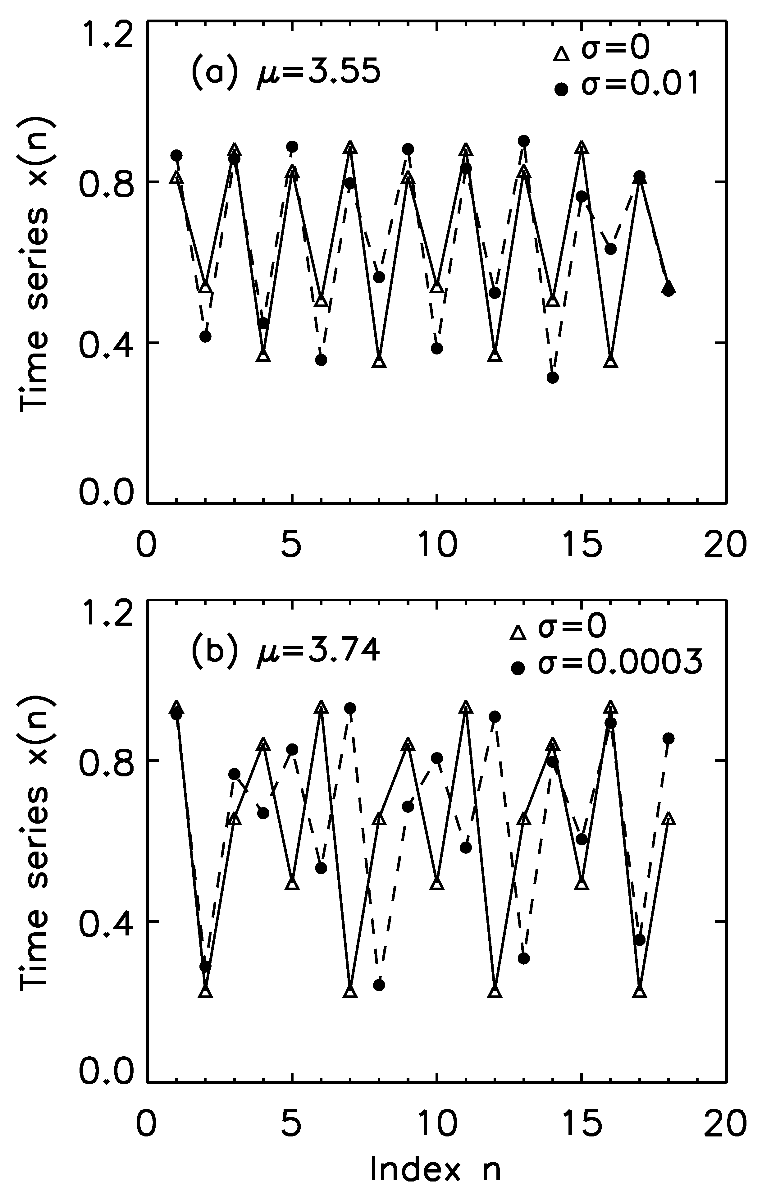
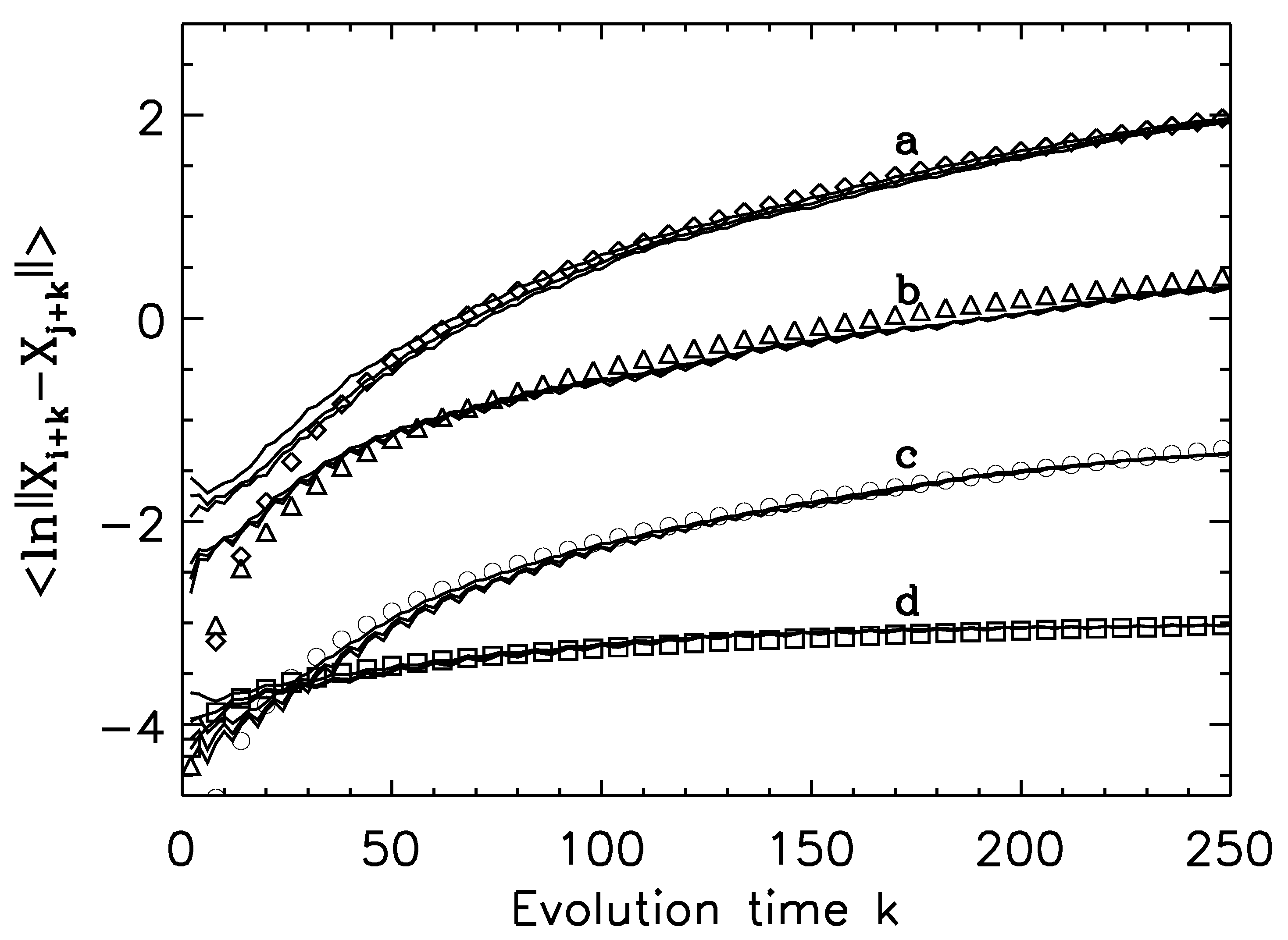
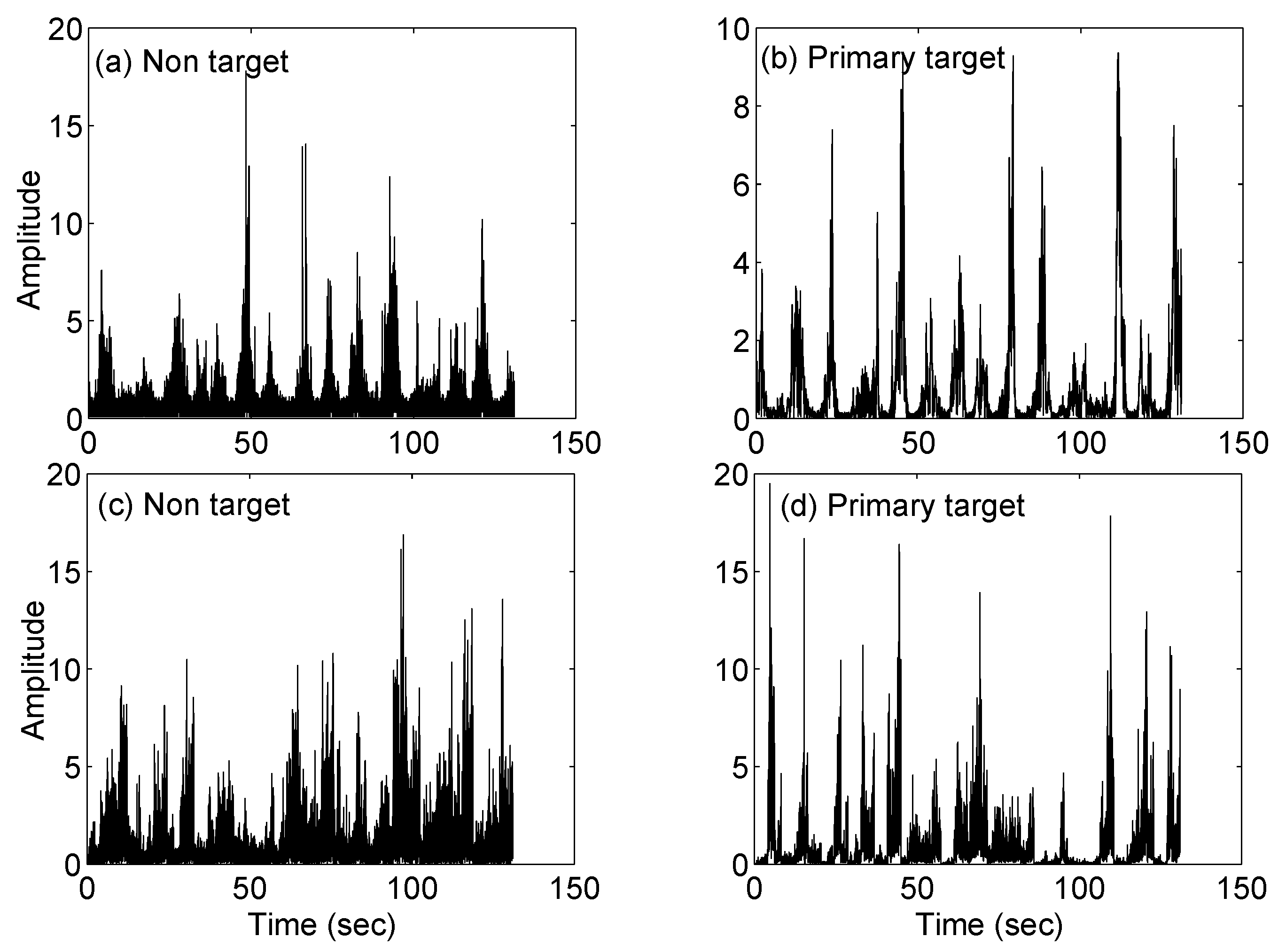
Here, $\mu$ is the bifurcation parameter, and $P_n$ is a zero-mean Gaussian random variable with standard deviation $\sigma$. When $P_n=0$, the map generates periodic orbits with periods 8, 6, 5, and 3 at parameter values $\mu =3.55$, 3.63, 3.74, and 3.83, respectively. The period-8 motion at $\mu =3.55$ is on the main $2^n$ cascade, and the period-3 motion at $\mu =3.83$ is on the period(3)-doubling cascade (see Figure 10). For the case of $\mu =3.55$, with a fairly large noise of $\sigma =0.01$, the noisy trajectory is still very similar to the clean period-8 trajectory, as one can clearly see from Figure 16a. The case of $\mu =3.74$ is very different. With $\sigma$ as small as 0.0003, the noisy trajectory is already completely different from the original clean period-5 trajectory, as shown in Figure 16b. In fact, this noisy trajectory is chaotic, as shown by the time-dependent exponent curves shown in Figure 17c. In contrast, the noisy dynamics at $\mu =3.55$ are definitely not chaotic, as shown by Figure 17a. The noisy dynamics at $\mu =3.63$ and 3.83 are also chaos-like, though not as well defined as at $\mu =3.74$. The mechanism for noise-induced chaos can be found by examining how a small amount of noise affects the dynamics. In general, the noisy dynamics when noise is very small is a diffusion characterized by Equation (44). The normal diffusion with $\alpha \approx 0.5$ corresponds to Brownian motions around the periodic orbit (or limit cycle), which is clear from Figure 16a. The case of super diffusion with $\alpha >0.5$ is the very condition for noise-induced chaos to occur. This is shown in Figure 18 and can be readily understood as follows: chaos, which amounts to exponential divergence, can be more easily approached through larger $\alpha$, especially when $\alpha$ is larger than 1, for a tiny amount of noise.

Let us now come back to chaotic secure communications. Although noise-induced chaos can help with chaos synchronization, and thus chaos communication, the noise level has to be small. Otherwise, chaotic systems will desynchronize, and we will not be able to have any kind of communication at all [82].

In the beginning of this subsection, we have mentioned that recently there is a strong interest in using chaos to rapidly generate random bits in physical devices, for use in cryptography and secure communication. For this purpose, noise is always beneficial. The key here is to test whether a generated sequence of 0’s and 1’s is truly random. The usual tests for randomness, such as the widely used Statistical Test Suite for random number generator of NIST SP 800-22, basically test whether the distributions of 0’s and 1’s in the entire and the sub-sequences, as well as recurrences of certain patterns, are consistent with certain random distributions. The degree of divergence of nearby trajectories characterized by the time-dependent exponent curves offer additional information [109]. This is best understood by referring to Figure 17: the noise-induced chaos at $\mu =3.74$ and 3.83 is more suitable to be used as fast physical random bit generator than at $\mu =3.63$. The normal diffusion-like process at $\mu =3.55$ will not pass the randomness test of NIST SP 800-22 since the dynamics are periodic-like.

Finally, as a side comment, we note that the pioneering works on chaos synchronization [100,101,102,103,104,105,106,107,108,109,110,111] are not cited evenly. Rather, some were only cited a few times, while the largest citation goes to [100], which is over 12,000 times. To better appreciate this somewhat astonishing behavior, we have listed these works in the reference not chronologically, but in descending order of the citations. The actual number of citations is shown in Figure 19, where the rank k from 1 to 12 denote references from [100,101,102,103,104,105,106,107,108,109,110,111]. Interestingly, the number of citations decays exponentially. This is in stark contrast with the behavior of the large-scale citation network mentioned earlier, which is a power law. This simple analysis has an interesting implication to using citation as a critical measure of the significance of scientific works. The analysis presented here clearly suggests that such a practice should not be taken too seriously, at least not taking citation as the sole measure of the significance of scientific works. In addition, there is an interesting lesson here: to enhance citations of one’s work, it is important to get further involvement in the later development of a subject, after producing some pioneering work. For example, Dr. Pecora and Carrol have been actively involved in fostering the development of chaotic secure communications. Finally, there is an interesting question from this simple analysis: Can we develop a model to reconcile the exponential decay of citation to pioneering works with general power law decay of citations?

2.4. Basics of Random Fractal Theory

In practice, many problems contain random elements. Random fractal theory is of crucial importance for finding structures and regularities in the random data, especially when the data involve a wide range of spatial and/or temporal scales (i.e., cover a long period of time or a wide extent of space).

Chaos and fractal theories are often discussed together and thought to be the same thing. This is a harmful perception because the part of fractal theory that is most useful for signal processing is the random fractal theory, whose foundation is fundamentally different from that of chaos theory. Chaos theory mainly studies irregular behaviors in nonlinear dynamical systems with only a few degrees of freedom. Here, noise or intrinsic randomness only has a minor role. Random fractal theory concerns systems that are inherently random. When equating chaos theory with fractal theory, one then will fail to fully understand the differences in the mathematics of the two theories, and fail to fully appreciate important issues such as distinguishing chaos from noise—a newcomer tackling the issue would think it sufficient to distinguish chaos from simple white noise. Unfortunately, this is not the case. Only if we can distinguish chaos from all known models of random processes can we say we can distinguish chaos from noise.

Below, we first discuss the basics of fractal theory, then we focus on random fractal theory. We will resume discussion of distinguishing chaos from noise in Section 2.5.

2.4.1. Introduction to Fractal Theory

Euclidean geometry studies simple shapes, including lines, planes, triangles, squares, cones, spheres, and so on. All these shapes are regular. Every one has seen clouds, mountains, and other complex shapes in nature. How well can those complex shapes be modeled by circles, spheres, cones, or other regular shapes? Very badly! When thinking along this line, Mandelbrot has created a new field, the fractal geometry [121].

Let us first try to understand fractal intuitively. The key here is self-similarity, which means that part of an object, when magnified, is similar to the whole. More concretely, whether we magnify the object by 10 times or 100 times, we always observe similar objects.

When discussing power laws, we have emphasized that a power law embodies self-similarity (please see Figure 2). Therefore, power law relations are natural mathematical tools to characterize fractals. When plotted in double-logarithmic scale, power laws become linear relations. To better appreciate the significance of power laws, imagine hiking on a mountain trail. Unlike many manmade trails with hundreds of stairs in the mountains of China, we assume the trail we are walking up is wild and irregular. How can we measure the distance we have walked? Let us measure the total distance by our step size. Denote it by $ϵ$. Note $ϵ$ could be different for different hikers—one who rides a horse has a huge step size, while a little baby surely only has a tiny step size. The distance we have walked up is then

$$L=N\left(ϵ\right)·ϵ,$$

(66)

where $N\left(ϵ\right)$ is the number of intervals walked. Amazingly, $N\left(ϵ\right)$ scales with $ϵ$ as a power law, just as described by Equation (23), where $1<D<2$ is not an integer. Such a nonintegral D is the celebrated fractal dimension of the hiking trail.

What is the meaning of a nonintegral D? To find the answer, we start from the measurement of certain length, area, or volume. The basics of calculus teach us that we can measure a curve, a surface area, or a volume using very small intervals, squares, or cubes by properly covering the object we are interested to measure. Take the unit length, unit area, or unit volume as the unit of measurement, with linear size $ϵ$. Now suppose we measure the length of a straight line with length 1. What is the minimal number of intervals of length $ϵ$ needed to fully cover this unit length? We need at least $N\left(ϵ\right)\sim {ϵ}^{-1}$ intervals. Extending to 2D and 3D, when covering an area or volume by boxes with linear length $ϵ$, we need at least $N\left(ϵ\right)\sim {ϵ}^{-2}$ squares to cover the area, and $N\left(ϵ\right)\sim {ϵ}^{-3}$ cubes to cover the volume. The D in $N\left(ϵ\right)\sim {ϵ}^{-D}$ here is called the topological dimension, which is 1 for a line, 2 for an area, and 3 for a volume. For M isolated points, the scaling law becomes $N\left(ϵ\right)=M{ϵ}^{-D}$, with $D=0$. Therefore, the topological dimension D for isolated points is zero. We thus see that when we call a point, a line, an area, and a volume $0-D$, $1-D$, $2-D$, and $3-D$ objects, we are talking about their topological dimensions.

We can now discuss the consequence of $1<D<2$ for an irregular mountain trail. Combining Equations (23) and (66), we have

$$L={ϵ}^{1-D},$$

(67)

Therefore, when $ϵ$ becomes smaller, L becomes larger. In fact, when $ϵ\to 0$, $L\to \infty$. This property was actually first found by Lewis Richardson, a mathematician, meteorologist, and pacifist who devoted himself in his later years to the study of the causes of wars and ways to prevent them. However, we have to wait for Mandelbrot to find the quantitative power law relation described by Equation (23), to create the new field of fractal.

With Equation (67), we can actually deduce more by using some concrete numbers. For example, let us take $D=1.25$, and imagine a race between a hare and a tortoise. Taking into account the physical difference between a hare and a tortoise, it it reasonable to assume that the step size of the hare is 16 times that of the tortoise. Then we have

$$L_{\mathrm{hare}}=\frac{1}{2}{L}_{\mathrm{tortoise}}$$

(68)

The tortoise has to crawl twice the distance that the hare runs! Based on this simple calculation, we now understand when we walk along a wild trail, get tired, slow down, we are actually shrinking our step sizes, so we will be walking out a longer trail!

Next, we consider the Cantor set, one of the prototypical fractal objects, so that we can appreciate the concept of fractal dimension better.

The standard Cantor set is obtained by first partitioning a line segment into three equal parts and deleting the middle one. This step is then repeated, deleting the middle third of each remaining segment iteratively. See Figure 20a. Note that such a process can be related to the iteration of a nonlinear discrete map. The removed middle thirds can be related to the intervals that make the map diverge to infinity, while the remaining structures are linked to the invariant points of the map. At the limiting stage, $n\to \infty$, the Cantor set consists of infinitely many isolated points. Consistent with isolated point(s) having dimension 0, the topological dimension here is 0. The length of the total segments removed is

$$\frac{1}{3}+2\times {\left(\frac{1}{3}\right)}^2+4\times {\left(\frac{1}{3}\right)}^3+\cdots =\frac{1}{2}\times \frac{2}{3}+\frac{1}{2}\times {\left(\frac{2}{3}\right)}^2+\frac{1}{2}\times {\left(\frac{2}{3}\right)}^3+\cdots =1$$

(69)

Therefore, the entire unit interval has been removed! Is the fractal dimension here the same as the topological dimension, which is 0?

To find out, let us focus on stage n. One needs $N\left(ϵ\right)=2^n$ boxes of length $ϵ={\left(\frac{1}{3}\right)}^n$ to cover the set. Hence, the fractal dimension for the Cantor set is

$$D=-lnN\left(ϵ\right)/lnϵ=ln2/ln3.$$

(70)

It is not zero!

The fractal dimension of the Cantor set can also be computed by employing the self-similar feature. Denote the number of intervals needed to cover the Cantor set at a certain stage with scale $ϵ$ by $N\left(ϵ\right)$. When the scale is reduced by 3, $N(ϵ/3)$ is doubled. Since $N(ϵ/3)/N\left(ϵ\right)=3^D=2$, one immediately gets $D=ln2/ln3$.

To better transit to random fractals, we note that the standard Cantor set can be made random. One way is to divide each interval into three equal parts and randomly delete one of them (see Figure 20b). An alternative way of obtaining a random Cantor set is to delete a middle interval of random length at each stage (Figure 20c). Clearly, case (b) also has dimension $D=ln2/ln3$. When certain regulation is imposed on the length distribution for the subintervals in case (c), the fractal dimension can also be readily computed. One way of imposing such a regulation is to require that the ratio of the subinterval and its immediate parent interval follows some distribution that is stage-independent. Such a regulation is essentially a multifractal construction, which we will discuss soon.

The above discussion suggests that two different geometrical fractals may have the same fractal dimension. To further appreciate this point, we have shown in Figure 20d a different type of regular Cantor set. It is obtained by retaining four equally spaced segments whose length is $1/9$th of the preceding segment. Denote the number of segments at a certain stage with length scale $ϵ$ by $N\left(ϵ\right)$. When the scale is reduced by 9, $N(ϵ/9)$ is quadrupled. Here, D is again $ln2/ln3$, since $N(ϵ/9)/N\left(ϵ\right)=9^D=4$.

Based on the above discussions, one can readily realize that fractal curves and surfaces are more space filling. This property is beneficial in biological evolution. As a result, fractal forms are abundant in biology. Instead of giving actual examples here, we will refer readers to reference [122] for a menagerie of fractal forms in living things. This more space-filling property of fractals has also been exploited to design fractal antennas by maximizing the effective length or perimeter of the material that receives or transmits electromagnetic radiation. Fractal antennas are excellent for wideband and multiband applications [123].

2.4.2. Overview of Random Fractal Theory

Gaussian white noise is the most extensively studied noise in engineering. In complex systems, however, the temporal or spatial fluctuations often cannot be modeled by Gaussian white noise. Rather, they are characterized by a power law decaying spectrum in the frequency domain, denoted as $1/f^{\alpha }$ noise [38]. Its dimensionality cannot be reduced by popular methods such as principle component analysis [124]. Interesting examples of such processes include genetics [125,126,127,128,129], human cognition [130] and coordination [131], posture [132], vision [133,134], physiological signals [80,135,136,137,138,139,140,141,142,143], neuronal firing [144,145], urban traffic [146], tree rings [147], global terrorism [148], human response to natural and social phenomena [149], foreign exchange rate [76], and the distribution of prime numbers [150].

Basic Definitions and Equations

Denote a covariance stationary stochastic process as $X=\{X_t:t=0,1,2,\dots \}$. Its mean is $\mu$, variance is ${\sigma }^2$, and autocorrelation function $r\left(k\right),k\ge 0$ has the following form

$$r\left(k\right)\sim k^{2H-2},ask\to \infty ,$$

(71)

where H is a parameter called the Hurst exponent. It is in the unit interval, $0<H<1$. The exponent $\alpha$ for the spectra of the process, $1/f^{\alpha }$, is related to H by a simple equation,

$$\alpha =2H-1.$$

(72)

When $0<H<1/2$, the process is said to have anti-persistent correlations; when $H=1/2$, the process is memoryless or only has short memory, when $1/2<H<1$, the process is said to have persistent long-range correlations. In this case, it is easy to prove ${\sum }_{k}r\left(k\right)=\infty$. This is why the process is said to have long-range correlation [38].

Let us now smooth the process X to obtain a time series $X^{\left(m\right)}=\{X_t^{\left(m\right)}:t=1,2,3,\dots \}$, $m=1,2,3,\dots$, where

$$X_t^{\left(m\right)}=(X_{tm-m+1}+\cdots +X_{tm})/m,t\ge 1.$$

(73)

The smoothing is carried out in a non-overlapping fashion; therefore, the length of $\{X_t^{\left(m\right)}\}$ is the largest integer that is not larger than $N/m$, where N is the length of $\left\{X_t\right\}$. Is there a relation between the variance of $X_t^{\left(m\right)}$, which is denoted by $V_m=var\left(X^{\left(m\right)}\right)$, and that of the original process, which is denoted by ${\sigma }^2$? It is given by

$$var(X^{\left(m\right)})={\sigma }^2{m}^{2H-2}$$

(74)

Equation (74) is often called the variance–time relation. It is fundamental and can help us understand the “little smoothing” phenomenon: when $H=0.5$, $var\left(X^{\left(m\right)}\right)={10}^{-2}{\sigma }^2$ when $m=100$. When $H=0.75$, for $var\left(X^{\left(m\right)}\right)$ to drop as much, m has to be 10,000. However, if $H=0.25$, then $var\left(X^{\left(m\right)}\right)\approx {10}^{-2}{\sigma }^2$ when $m\approx 23$. Therefore, when H increases to 1, smoothing has little effect in reducing the variance of the process.

As we have mentioned, the power spectral density (PSD) for X is

$$S_X\left(f\right)\sim f^{-\alpha }=f^{-(2H-1)}.$$

(75)

The integration of the X process, called the random walk process,

$$y_k=\sum _{i=1}^k(X_i-\overline{X}),$$

(76)

where $\overline{X}$ is the mean of X, has a PSD

$$S_Y\left(f\right)\sim f^{-\alpha -2}=f^{-(2H+1)}.$$

(77)

It is easy to see that the following relation is equivalent to Equation (74)

$$〈{|y(i+m)-y\left(i\right)|}^2〉\sim m^{2H},$$

(78)

where the angle brackets denote averaging over i. Equation (78) is often called fluctuation analysis (FA). The superiority of Equation (78) over Equation (74) is that it can be readily generalized to a multifractal formulation.

The Fractional Brownian Motion (fBm) Process

The fBm process is the prototypical random walk model for $1/f^{\alpha }$ process [121]. It is a zero-mean Gaussian process, with stationary increments and variance

$$E[{\left(B_H\left(t\right)\right)}^2]=t^{2H}$$

(79)

and covariance:

$$E\left[B_H\left(s\right)B_H\left(t\right)\right]=\frac{1}{2}\{s^{2H}+t^{2H}{-|s-t|}^{2H}\}$$

(80)

where H is the Hurst parameter. The increment process of the fBm, $X_i=B_H((i+1)\Delta t)-B_H(i\Delta t),i\ge 1$, where $\Delta t$ amounts to a sampling time, is called the fractional Gaussian noise (fGn). It is a zero-mean stationary Gaussian time series, with autocorrelation function:

$$\gamma \left(k\right)=E\left(X_i{X}_{i+k}\right)/E\left(X_i^2\right)=\frac{1}{2}\left\{{(k+1)}^{2H}-2k^{2H}+{|k-1|}^{2H}\right\},k\ge 0$$

(81)

Note $\gamma \left(k\right)$ is independent of $\Delta t$. In particular, $\gamma \left(1\right)=\frac{1}{2}\left(2^{2H}-2\right)$. It is positive when $1/2<H<1$, and negative when $0<H<1/2$. When $k\to \infty ,\gamma \left(k\right)\sim k^{2H-2}$, and we reproduce Equation (71).

Structure Function Based Multifractal Analysis

Since the Hurst parameter H is the defining parameter of random fractals, it is certainly of critical importance to estimate H. To facilitate estimation of H, it is most convenient to use the random walk process y, defined by Equation (76), and consider the following multifractal formulation:

$$F^{\left(q\right)}\left(m\right)={〈{|y(i+m)-y\left(i\right)|}^q〉}^{1/q}\sim m^{H\left(q\right)},$$

(82)

where q is real-valued. The average is taken over all possible pairs of $\left(y\right(i+m),y(i\left)\right)$. Note that $q>0$ highlights large absolute value of $\left|y\right(i+m)-y(i\left)\right|$, while $q<0$ highlights small absolute value of $\left|y\right(i+m)-y(i\left)\right|$ (to understand better, it is beneficial to take $q=10$ and $ma{x}_i|y(i+m)-y\left(i\right)|=100$, and $q=-10$ and $mi{n}_i|y(i+m)-y\left(i\right)|=1/100$). $H\left(q\right)$ is a non-decreasing function of q. When $H\left(q\right)$ is a constant, the process is called a monofractal; otherwise, it is a multifractal.

Note that when $q=2$, Equation (82) reduces to Equation (78), the FA, and $H\left(2\right)=H$. It can be readily proven that FA is equivalent to many other methods for estimating H, including the variance–time relation, the Fano factor analysis, and a few others [38,151] (the H value estimated by the R/S statistic is equivalent to $H\left(1\right)$). While all these methods are important, they have a limitation in that the largest H estimated by them is 1. Many processes, including auto-regressive processes, ON/OFF models, Levy walks, and processes with trends, have $H>1$ on some time scale range. To accurately estimate those exponents, one has to use other methods, such as detrended fluctuation analysis (DFA) [152] and wavelet multi-resolution analysis [153]. In Section 3, we will present an improvement of DFA, adaptive fractal analysis (AFA) [149,154,155,156,157].

Singular Measure Based Multifractal Analysis

There is an alternative multifractal formalism to the structure-function based technique. It is based on probabilities and the thermodynamic formulation. The basic idea is to consider the scaling behaviors for the qth moments of the measure $\mu$ [38,153]:

$$Z(q,ϵ)=\sum _{i=1}^{N\left(ϵ\right)}{\mu }_i^q\left(ϵ\right)\sim {ϵ}^{\tau \left(q\right)},ϵ\to 0$$

(83)

where $N\left(ϵ\right)$ is the minimal number of boxes of linear size $ϵ$ that are used to cover the support of the measure $\mu$. The spectrum of the generalized dimensions $D_q$ is defined by

$$D_q=\frac{\tau \left(q\right)}{q-1},$$

(84)

Comparing with our discussions on the $D_q$ spectrum for chaotic systems, we readily see that $D_0$ is the capacity (or box-counting) dimension, and $D_1$ is the information dimension. Just as the $H\left(q\right)$ spectrum, $D(q$) is a non-decreasing function of q. When $D\left(q\right)$ is constant in q, the measure is called monofractal; otherwise, it is called multifractal.

There is another interesting way to characterize the properties of the measure. It is by the singular spectrum $f\left(\alpha \right)$, where $\alpha$ is called the pointwise dimension. The basic equation connecting the two characterizations is the Legendre transform,

$$q=df\left(\alpha \right)/d\alpha ,\tau \left(q\right)=q\alpha -f\left(\alpha \right).$$

(85)

Combining Equations (84) and (85), we have

$$D_q=\frac{1}{q-1}[q\alpha \left(q\right)-f\left(\alpha \left(q\right)\right)].$$

(86)

We thus see that $D_q$ and $f\left(\alpha \right)$ provide the same amount of information.

The Random Cascade Model

In the study of multifractals, it is important to have a constructive model. This is provided by the random cascade model. It is among the most powerful models to understand the intermittency phenomenon of turbulence [158,159,160,161,162]. Here, we will use the notations developed for modeling Internet traffic and geophysical data [38,163,164,165] to present the model.

Consider a unit mass unevenly distributed on a unit interval. Let us divide the unit interval into two parts: call them the left and the right segments. By doing so, we have also partitioned the mass into two fractions, r and $1-r$, which are on the left and right segments correspondingly. In general, the multiplier r is a random variable, having a probability density function (PDF) $P\left(r\right)$, $0\le r\le 1$. Always with this rule we can further partition each new subinterval and the weight attached to it into two parts, ad infinitum. Figure 21 shows the procedure schematically. To facilitate mathematical analysis, the multiplier r has been rewritten as $r_{ij}$, where i indicates the stage number and j indicates the positions of a weight on that stage (we only use odd numbers, leaving even numbers for $1-r_{ij}$). For many types of data analysis, it is important to explicitly introduce the notion of scale. This is provided by the interval length, which is $2^{-i}$ at stage i. Assuming bilateral symmetry, then we have to require that $P\left(r\right)$ is symmetric about $r=1/2$. Let $P\left(r\right)$ have successive moments ${\mu }_1,{\mu }_2,\cdots$. Hence, $r_{ij}$ and $1-r_{ij}$ both have marginal distribution $P\left(r\right)$. The weights at the stage N, $\{w_n,n=1,\dots ,2^N\}$, can be expressed as

$$w_n=u_1{u}_2\cdots u_N,$$

(87)

where $u_l$, $l=1,\cdots ,N$, are either $r_{ij}$ or $1-r_{ij}$. Thus, {$u_i,i\ge 1$} are IID random variables all having PDF $P\left(r\right)$.

The cascade model has many interesting properties. We list a few here:

• The weights at stage N are log-normally distributed. To see this, one can take logarithm on both sides of Equation (87), then the multiplication becomes summation, and one can use the central limit theorem.
• We can readily derive that

  $$\tau \left(q\right)=-ln\left(2{\mu }_q\right)/ln2.$$

  (88)
• We can also derive that

  $$H\left(q\right)\sim -\frac{1}{q}ln{\mu }_q/ln2,$$

  (89)

  and

  $$\tau \left(q\right)=qH\left(q\right)-1.$$

  (90)

We now illustrate Equations (88) and (89) using an example, the random binomial model, whose $P\left(r\right)$ is

$$P\left(r\right)=\left[\delta \right(r-p)+\delta (r-(1-p)\left)\right]/2$$

(91)

where $\delta$ denotes the Dirac function. Therefore, $P(r=p)=P(r=1-p)=1/2$. Here, the qth moment ${\mu }_q=[p^q+{(1-p)}^q]/2$. We thus find

$$\tau \left(q\right)=-ln[p^q+{(1-p)}^q]/ln2$$

(92)

and

$$H\left(q\right)=\frac{1}{q}\{1-ln[p^q+{(1-p)}^q]/ln2\}$$

(93)

Clearly, $H\left(q\right)$ is a non-decreasing function of q. Without loss of generality, we may take $p\le 1//2$. When $q\to -\infty$, H converges to its tight upper bound of $-lnp/ln2>1$. When $q\to \infty$, H converges to its tight lower bound of $-ln(1-p)/ln2<1$.

In the cascade model, many different functional shapes for $P\left(r\right)$ can be used [163,164], and the model can simulate a random function with very high accuracy. Two examples are shown in Figure 22 for sea-clutter amplitude data [38,166]. The model can also be readily generalized to the high-dimensional case. The case for 2D is shown in Figure 23.

2.5. Going from Distinguishing Chaos from Noise to Fully Understanding the System Dynamics

A long-standing problem in time series analysis, which is still of interest today, is to distinguish chaos from noise. This problem naturally arises when one wishes to understand whether certain complex behaviors in physics, finance, life sciences, ecology, and other fields, are of deterministic origin, or genuinely random. An unambiguous answer to the question can greatly help one to choose a proper model to study the behavior one wishes to understand. For a long time, however, when one computes a nonintegral fractal dimension, or a positive largest Lyapunov exponent, or a finite Kolmogorov entropy from a time series, one would think the time series is chaotic. In many applications, many researchers are still assuming so! Is this a sound assumption? Unfortunately, it is not. As one can expect, the most convincing counter-example would be the one that a genuinely random time series is interpreted as deterministic chaos by this assumption. It turns out that all $1/f^{\alpha }$ random processes can be proven to have non-integral fractal dimensions of $1/H$ [38], and finite Kolmogorov entropies [167,168], and thus may be misclassified as chaos. Because of this problem, it is desirable that whenever one studies chaos in observational data, one explicitly tests whether the data truly have the signature of chaos, the exponential divergence. In Section 4, we will discuss the scale-dependent Lyapunov exponent (SDLE), which generalizes the notion of the Lyapunov exponent. We will see there that SDLE can readily solve the problem.

Nowadays, efforts are still being made to develop innovative methods to distinguish chaos from noise. In our view, it is more important to find the defining parameters of the complex time series that one studies. In particular, one has to ask: If the time series is truly chaotic, what is the exponential growth rate? If the time series is random, what type of randomness is it? Only if we can unambiguously answer these fundamental questions can we truly understand the system under study. Clearly, this is more than simply trying to distinguish chaos from noise. In doing so, one will find that chaos and random fractals may both play significant roles in one’s problem: chaos and random fractal may be manifested on different scales. This is the essence of multiscale phenomena: signals may exhibit different quantifiable features on different scales. Therefore, to best characterize a complex system, we need to use a number of tools synergistically. With this rationale, another fundamental question arises: what are the relations among the different complexity measures?

We have already introduced a number of different complexity measures, including the largest positive Lyapunov exponent, fractal dimension, generalized dimension spectrum, Kolmogorov–Sinai entropy, correlation dimension, correlation entropy, sample entropy, and multiscale entropy. Before discussing the connections among these complexity measures, we explain a few more measures, including the Lempel-Ziv (LZ) and the Kolmogorov–Chaitin complexity.

The LZ complexity is asymptotically equivalent to the Shannon entropy. The algorithm for computing the LZ complexity can be efficiently implemented and executed, and thus the LZ complexity and its many derivatives have found wide applications—the value of the LZ complexity of a numerical, text, or image file may be equated to the size of their compressed files using the commonly used compression schemes. To compute the LZ complexity for a time series, it is important to consider the effect of the finite length of the data. For more details, we refer to [169].

The Kolmogorov–Chaitin complexity is also called descriptive complexity, Kolmogorov complexity, algorithmic complexity, algorithmic entropy, and program-size complexity. It is a key measure in algorithmic information theory. The Kolmogorov–Chaitin complexity of a string of numbers or a text file is the length of the shortest computer program that generates the the string of numbers or the text file. Therefore, it measures the computational resources needed for specifying an object. To make the above discussions concrete, one can think of a completely random string. It is impossible to compress the string into a program with length shorter than the length of the string itself; the simplest program is to just read out the string. Although the lower bound for the Kolmogorov–Chaitin complexity of an object is difficult to obtain [20], the upper bound is easy to get, which are just the Shannon entropy or the LZ complexity. For dynamical systems and Markov information sources, this upper bound can almost surely be achieved [170].

Next, we explain a widely used entropy measure, the approximate entropy. The approximate entropy amounts to taking $q=1$ in Equation (55) at a fixed scale $ϵ$ and two small embedding dimensions (say $m_0$ and $m_0+1$) instead of taking the limits of ${lim}_{ϵ\to 0}$ and ${lim}_{m\to \infty }$. While it is closely related to the sample entropy, it is not as effective as the sample entropy in resolving the scaling behavior. This is part of the reason that multiscale entropy is built op top of the sample entropy. For more details, we refer to [171].

Finally, we explain the permutation entropy (PE) [172]. Due to its simplicity, it has found numerous applications in time series analysis. Here, we describe PE following the notations of [173].

We start from an m-dimensional embedding vector, $X_i=[x\left(i\right),x(i+L),\cdots ,x(i+(m-1)L)]$. Let us sort the elements of the vector in ascending order, $[x(i+(j_1-1)L)\le x(i+(j_2-1)L)\le \cdots \le x(i+(j_m-1)L]$. When an equality occurs, e.g., $x(i+(j_{i1}-1)L)=x(i+(j_{i2}-1)L)$, we choose their natural order, i.e., if $j_{i1}<j_{i2}$, then $x(i+(j_{i1}-1)L)\le x(i+(j_{i2}-1)L)$. This way, the vector $X_i$ is mapped onto a sequence of numbers, $(j_1,j_2,\cdots ,j_m)$. Permutating it, we see that there are a total of $m!$ distinct combinations of $(j_1,j_2,\cdots ,j_m)$. Each permutation can be considered as an m-dimensional symbol. Therefore, the reconstructed trajectory in the m-dimensional space is mapped to a m-dimensional symbol sequence. Let $P_1,P_2,\cdots ,P_K$ be the probability for the $K\le m!$ distinct symbols. The PE, denoted by $E_p$, for the time series $\left\{x\right(i),i=1,2,\cdots \}$ is defined as

$$E_p\left(m\right)=-\sum _{j=1}^K{P}_{j}ln{P}_j.$$

(94)

The maximum of $E_P\left(m\right)$ is $ln(m!)$ when $P_j=1/(m!)$. It is convenient to normalize it to obtain

$$0\le E_p=E_p\left(m\right)/ln(m!)\le 1.$$

(95)

$E_p$ essentially measures the randomness of the time series under study: with the passing of time, if data measured from a system become more regular, then $E_p$ of the corresponding data becomes smaller. This statement suggests that if one wishes to detect dynamical changes in a system, one can partition a time series into short windows, compute PE for each window, and examine how PE changes with the window [173].

The construction of PE may be considered a generalization of symbolic dynamics of dynamical systems for finite data, recalling that the essence of symbolic dynamics is to map a trajectory in certain space to a few subspaces, such as a trajectory defined in the unit interval $\left[01\right]$ to two sub-intervals, $[01/2)$ and $[1/21]$. The usefulness of symbolic dynamics is a strong hint that PE is often very useful for analyzing complex time series.

While the connections among some of the complexity measures discussed here are obvious, a more comprehensive answer also exists. This, however, has to wait until we introduce a new complexity measure, SDLE, in Section 4.

3. Adaptive Detrending, Denoising, Multiscale Decomposition, and Fractal Analysis

Observational data may manifest both ordered and disordered behavior. To fully characterize a complex signal, it is desirable to synergistically use chaos and random fractal theory [38]. However, this goal is not easy to achieve, since a measured data set often contains noise and may also be nonstationary. This makes detecting chaos very difficult. On the other hand, many phenomena contain a rhythmic activity, such as diurnal cycle. This makes fractal analysis difficult since the essence of a fractal is scale-free. To tackle these problems, frequency-domain filtering and wavelet analysis have been widely used to filter away the undesired features in the data. With the rapid accumulation of complex data in all branches of science and engineering, it is important to have better approaches to solve these problems. In this section, we discuss an adaptive algorithm, which has a number of interesting properties: (1) it can accurately determine a trend in the signal; depending on the purpose of applications, one may treat the trend and associated nonstationarities as noise, and remove them, or retain them, as the signals one wishes to further study (such as the global warming trend); (2) it is more superior in reducing noise in the signals than linear filters, wavelet methods, and chaos-based methods; (3) it can conveniently decompose a complex signal into many functions of different frequency; (4) it is excellent in obtaining fractal properties from the data, especially when the data contain a strong and nonlinear trend. The method has been successfully applied to study traffic flow [146,174], various kinds of geophysical data including soil temperature, soil moisture, air temperature, and wind speed [175,176,177,178], tree rings [147], variation of electricity consumption with time [179], single neuron firing [145], clinical scalp EEG [180], ngram usage [149], quantum modeling of exciton diffusion in light harvesting systems [181], sentiments in novels [182,183], newspaper advertisements [184], textual cultural heritage [185], and global terrorism [148]. The method will be very useful for analyzing various kinds of geophysical time series that have been rapidly accumulating in recent years. Here, we will only present the key elements of the method; a concrete example of combining this method with a machine-learning method (random forest) for distinguishing epileptiform discharges from normal electroencephalograms can be found in Li et al. [180].

3.1. Adaptive Detrending, Denoising, and Multiscale Decomposition

The method is based on adaptive filtering [149,155,156,186]. It works this way: first we partition a time series into many segments. Let the length of each segment be $w=2n+1$ points, and neighboring segments overlap by $n+1$ points. As we will see later, using segments with length containing odd number of sample points ensures symmetry. This operation also introduces a time scale $\frac{w+1}{2}\tau =(n+1)\tau$, where $\tau$ is the sampling time. For each segment, whose sample points represent a small portion of the curve we are studying, we assume the curve can be approximated by its Taylor series expansion very well. This suggests us to fit the segment by a polynomial of order M. Minimizing the error, the obtained polynomial fitting becomes the best local fitting. Here, an important parameter is the polynomial order M. When $M=0$, the fitting is piece-wise constant. When $M=1$, the fitting is locally linear (not necessarily also globally linear). Let $y^{\left(i\right)}\left(l_1\right),y^{(i+1)}\left(l_2\right)$, $l_1,l_2=1,\cdots ,2n+1$ be the fitted polynomial for the i-th and $(i+1)$-th segments. The fitting for the overlapped part of the two adjacent segments can be obtained by properly combining these two polynomials:

$$y^{\left(c\right)}\left(l\right)=w_1{y}^{\left(i\right)}(l+n)+w_2{y}^{(i+1)}\left(l\right),l=1,2,\cdots ,n+1$$

(96)

The two weights, $w_1=(1-\frac{l-1}{n}),w_2=\frac{l-1}{n}$, can be written as $(1-d_j/n),j=1,2$, where $d_j$ are the distances of the point from the centers of the two fitted polynomials. Therefore, the weights decrease linearly with the distance from the center of the segment. The weighting ensures symmetry. The scheme ensures that the overall fitted curve is continuous everywhere, has the right- or left-derivatives at the boundary, and is differentiable at non-boundary points.

The adaptive filter can readily determine any kind of trend from the data. An example for determining the trend from the global annual sea surface temperature (SST) data is shown in Figure 24a, where the blue straight line is the global linear fit, the black curve is the global second-order polynomial fit, and the red curve is the adaptive trend with a window size about the half of the total data length. It is amazing that with such a large window size, not only the global warming trend but also the local brief cooling periods are clearly shown. In fact, the residual noise (i.e., the difference between the fitting and the original data) shown in Figure 24b with these fits is comparable to that obtained by empirical mode decomposition (EMD) [187]. Since EMD involves dyadic decomposition, while the window size used by the adaptive method is continuous, the adaptive filtering is more flexible and can be accurate.

Note that whether the trend is considered noise or the desired signal depends on one’s purpose. When the trend is considered noise, the approach is a high-pass filter. When the trend signal is considered the desired signal, then the approach is a low-pass filter. We can also take two window sizes and determine two trend signals. If we take the difference between them, then the approach becomes a band-pass filter. More generally, if we use a series of window sizes, $w_1=2n_1+1<w_2=2n_2+1<w_3=2n_3+1<\cdots$ and get the corresponding trend signals. The difference between the two trend signals of window sizes $w_i=2n_i+1$ and $w_j=2n_j+1$ is called a band-limited signal, with cutoff frequencies $1/\left(n_i\tau \right)$ and $1/\left(n_j\tau \right)$, where $\tau$ is the sampling time. These signals are called intrinsically band limited functions (IBFs) [154]. For an interesting application of the scheme (removing an ECG component from an EEG measurement for the study of apnea), we refer to [156].

The adaptive filter discussed here is more effective than linear filters, the wavelet method, and chaos-based approaches in reducing noise [155,156]. To see this, we have shown a comparison of these methods in Figure 25 for reducing measurement noise in the chaotic Lorenz system. The residual noise, characterized by the root-mean-square error (RMSE), is the smallest for the adaptive filter [154].

To better appreciate the above discussed properties of the filter, let us consider a power load time series measured at a power plant in Guilin during a long time period (from 1 January 2005 to 29 April 2010). Guilin is a very well-known tourism city, with the saying “Guilin’s landscape is the most uniquely beautiful in the world”. Power load time series may be equated to electricity consumption in a city. Interesting questions one can ask include whether electricity consumption may be correlated with climate variations. The raw load time series from Guilin is shown in Figure 26a as the blue curve. Here, the sampling time is 15 min. We observe that the data are very irregular and non-stationary, reflecting that the city’s businesses and population must have been changing a lot during the period the data were collected. The trend signal for the raw data is shown in Figure 26a as the red curve; it is obtained by using a window size of 699 sample points. The order of the polynomial used for fitting is 2 (if the raw signal is very spiky, then higher-order polynomials are recommended).

To facilitate further discussion, we denote the raw data by $x\left(t\right)$, and the trend signal by $trend\left(t\right)$. Then we have

$$x_{detrended}=x\left(t\right)-trend\left(t\right)$$

(97)

In order to see the details of $x_{detrended}$, Figure 26b shows a small segment of it as the blue curve. We observe a diurnal cycle in the data. This is reasonable since electricity consumption in daytime and during night has to be quite different. The signal does not have a fixed amplitude though, as it is still quite noisy. This noise, which is high frequency, can also be removed by applying the adaptive filter again, with a small window size. The trend thus determined will better represent the diurnal cycle. It is a band-pass signal. An example of this signal is shown in Figure 26b as the red curve, where we used a window size of 9 and a polynomial of order 2. From this signal, we can construct a phase diagram with delayed coordinates. This is shown in Figure 26c. A limit cycle-like structure does emerge.

We can further analyze the oscillatory feature of the trend signal by computing power-spectral density (PSD) from the data. The result is shown Figure 26d, where the blue, red, and green curves are for the raw, detrended, and the band-passed signals, respectively. The PSD curves show very sharp spectral peaks at frequency of 1 day${}^{-1}$ and its harmonics. Note the blue curves are basically covered by the other two colors, except at the very low frequency (i.e., close to 0 Hz). This is due to the red trend signal shown in Figure 26a.

3.2. Adaptive Fractal Analysis (AFA)

In the past three decades, many efforts have been made to estimate H, the most important parameter for random fractals. As a result, many excellent methods for estimating H have been proposed. Among them is the celebrated detrended fluctuation analysis (DFA) [151,152]. It works as follows: To analyze a time series, $x_1,x_2,x_3,\cdots$, one first determines its mean $\overline{x}$, then constructs a random walk process using Equation (76). By doing so, one has assumed that the data are like a noise process. One then partitions the random walk into non-overlapping segments of length l (therefore, the number of distinct segments is not larger than $N/l$, where N is the length of the time series). One furthers determines the local trend in each segment by using the best linear or polynomial fitting. This procedure is schematically shown in Figure 27, where a short EEG signal is used as an example. Finally, one obtains the difference between the original “walk” and the local trend. Denote it by $u\left(n\right)$. H is then estimated by

$$F_d\left(l\right)={\langle \sum _{i=1}^l{u}_l{\left(i\right)}^2\rangle }^{1/2}\sim l^H$$

(98)

where the angle brackets is a short-hand notation for averages over all the segments.

Although DFA is very good in many applications, when a signal has a strong nonlinear trend, such as an oscillatory component or a rhythmic activity, there may exist large discontinuities in adjacent segments of DFA (see Figure 27). These discontinuities can cause big problems. This problem can be readily solved by the adaptive fractal analysis (AFA) [149,154,157]. The difference with DFA is that we now have a globally, not only continuous but also almost everywhere, differentiable trend [155,156]. Denote it by $v\left(i\right)$. The difference between the original random walk process $u\left(i\right)$ and $v\left(i\right)$ can be used to accurately estimate H. The formula is given by [154]

$$F\left(w\right)={\left[\frac{1}{N}\sum _{i=1}^N{(u\left(i\right)-v\left(i\right))}^2\right]}^{1/2}\sim w^H.$$

(99)

Generalizing to a multifractal analysis, we obtain:

$$F^{\left(q\right)}\left(w\right)={\left[\frac{1}{N}\sum _{i=1}^N{|u\left(i\right)-v\left(i\right)|}^q\right]}^{1/q}\sim w^{H\left(q\right)}$$

(100)

where q is a real number. Just as we have discussed earlier, positive q values highlight large values in $\left|u\right(i)-v(i\left)\right|$, and negative q values highlight small values in $\left|u\right(i)-v(i\left)\right|$.

Equation (99) can readily be extended to long-range cross-correlation analysis [188] between two series: $x\left(i\right),i=1\cdots ,n$ and $y\left(i\right),i=1\cdots ,n$. Denote their trend signals corresponding to window size w by $\mathrm{trend}\_x^{\left(w\right)}\left(i\right),i=1\cdots ,n$ and $\mathrm{trend}\_y^{\left(w\right)}\left(i\right),i=1\cdots ,n$, respectively. Then we have

$$F_{xy}\left(w\right)={\left[\frac{1}{N}\sum _{i=1}^N(x\left(i\right)-\mathrm{trend}\_x^{\left(w\right)}\left(i\right))\times (y\left(i\right)-\mathrm{trend}\_y^{\left(w\right)}\left(i\right))\right]}^{1/2}\sim w^{H_{xy}}.$$

(101)

Following the generalization from Equations (99)–(100), Equation (101) can also be readily extended to multifractal analysis.

Let us now examine the fractal behavior of the power load data of Figure 26a using AFA. To cope with the nonstationary of the data, we partition the data into short windows, then we estimate H for each window. Recalling that the data are sampled 96 times a day, we choose the window size to be one month, containing $96\times 30=2880$ sample points. To improve the resolution of the variation of H, the adjacent windows overlap by half of the window length. Figure 28a shows an example of the scaling analysis using AFA, for an arbitrarily window. The curve is linear for scale up to $w=2^7$ sample points. It is a little longer than a day. H can be estimated as the slope of the linear portion of the curve. The temporal variation of H is plotted in Figure 28b as the red curve. Interestingly, it has a seasonal variation. To check whether this variation may be correlated with the yearly temperature variation, we have also shown in Figure 28b a curve in black reflecting the temperature variation. To facilitate comparison of the two variables, H and the temperature T, in the same plot, T is transformed to $T^{\prime }$ according to the following equation,

$$T^{\prime }=T/100+0.5.$$

(102)

Interestingly, the local maxima of the $H\left(t\right)$ curve correspond to the seasonal minima of the curve for the temperature. This suggests that the power load data are characterized by stronger, persistent, long-range correlations during winter.

4. Multiscale Analysis with the Scale-Dependent Lyapunov Exponent (SDLE)

SDLE is developed for better distinguishing chaos from noise and for better characterizing complex data, especially through obtaining the defining parameters of the data [38,189]. SDLE is closely related to two other methods, the time-dependent exponent curves [73,74,79,81] and the finite size Lyapunov exponent [190,191,192]. SDLE was first introduced in [38,189], and has been further developed in [193,194] and applied to characterize EEG [143], HRV [195,196], financial time series [76], Earth’s geodynamo [197], precipitation dynamics [198], sea clutter [199], THz imagery [200], and evaluate randomness [99]. As with the presentation of AFA, here, we will only present the key elements of the method; a concrete example of combining this method with a machine-learning approach (random forest) for distinguishing epileptiform discharges from normal electroencephalograms can be found in Li et al. [201].

SDLE is based on the evolution of vectors in a high-dimensional phase space. If initially the data are a time series, then one needs to obtain a suitable phase space using delay coordinates, as explained before. If the original data are a scalar random process, then the main advantage of the embedding procedure is to obtain a self-similar vector process from the original self-affine process. This is because x and t have different units and therefore have to be scaled differently in order for them to look “alike”. All the components of a vector are of the same nature, and therefore can be stretched or shrunk with the same fashion. Consequentially, whenever a truly random time series is analyzed, the specific value of the embedding dimension m is not important. Often ensuring $m>1$ is sufficient. After a phase space is obtained, one can examine the evolution of an ensemble of trajectories. Denote the initial distance between two nearby trajectories by ${ϵ}_0$. We further denote their average distance at time t by ${ϵ}_t$, and that at $t+\Delta t$ by ${ϵ}_{t+\Delta t}$. A schematic showing how a small distance between two nearby trajectories grows with time is shown in Figure 29. With this setting, we can examine the relation between ${ϵ}_t$ and ${ϵ}_{t+\Delta t}$, where $\Delta t$ is assumed to be small. When $\Delta t\to 0$, we have,

$${ϵ}_{t+\Delta t}={ϵ}_t{e}^{\lambda \left({ϵ}_t\right)\Delta t},$$

(103)

where $\lambda \left({ϵ}_t\right)$ is the SDLE given by

$$\lambda \left({ϵ}_t\right)=\frac{ln{ϵ}_{t+\Delta t}-ln{ϵ}_t}{\Delta t}.$$

(104)

Equivalently, we can write,

$$\frac{d{ϵ}_t}{dt}=\lambda \left({ϵ}_t\right){ϵ}_t.$$

(105)

Now that we have introduced SDLE, we can better understand the classic algorithm for computing the largest Lyapunov exponent ${\lambda }_1$ discussed earlier [75]. That algorithm assumes ${ϵ}_t\sim {ϵ}_0{e}^{{\lambda }_{1}t}$ and then through averaging estimates ${\lambda }_1$ by $(ln{ϵ}_t-ln{ϵ}_0)/t$. This assumption may not even hold for true chaotic signals. This is reminded in the detail of the schematic plot shown in Figure 29 —${ϵ}_{t+\delta t}$ may be smaller than ${ϵ}_t$. As already mentioned, a fundamental difficulty with this assumption is that for any type of noise, when ${ϵ}_0$ is small (which is the case when nearest neighbors are used), ${\lambda }_1$ can always be positive, leading to misinterpreting noise as chaos. The reason is simple: ${ϵ}_t$ will rapidly converge to the most probable distance between the constructed vectors, and thus will almost be surely larger than ${ϵ}_0$. However, when we define SDLE using Equation (103), we have not made any assumptions, except $\Delta t$ being small (usually taken to be the sampling time interval). As we will see, chaos is characterized by a constant $\lambda \left(ϵ\right)$ over a range of $ϵ$.

In the computation of SDLE, we first examine which embedding vectors defined by Equation (32) fall within the series of shells defined by Equation (40). Then, the evolution of those vector pairs $(V_i,V_j)$ can be monitored, and their average behavior of divergence (not necessarily exponential) can be computed. So far as exponential or power law divergence are concerned, we can exchange the order of taking the logarithm and averaging. Then, Equation (104) becomes

$$\lambda \left({ϵ}_t\right)=\frac{〈ln\parallel V_{i+t+\Delta t}-V_{j+t+\Delta t}\parallel -ln\parallel V_{i+t}-V_{j+t}\parallel 〉}{\Delta t}$$

(106)

where t and $\Delta t$ are measured in terms of the sampling time, and the average, denoted by the angle brackets, is over all indices $i,j$ with their corresponding vectors satisfying Equation (40).

The program for computing SDLE is explained in detail in [202], and can be obtained from the authors. The major scaling laws of SDLE that are most relevant for analyzing complex data are summarized below [189]:

• For deterministic chaos,

  $$\lambda \left(ϵ\right)\sim \mathrm{constant},$$

  (107)
  Amazingly, this property can even be observed in finite high-dimensional data, including the Lorenz’96 system, which has dimensions close to 30 [193], and in turbulent isotropic fluid with an integral scale Reynolds number reaching 6200 [203]. In such systems, estimation of dimensions is infeasible.
• As observational data are always contaminated by noise, it is important to have a scaling law for noisy chaos and noise-induced chaos [82,118]. The law reads

  $$\lambda \left(ϵ\right)\sim -\gamma lnϵ,$$

  (108)
  The law pertains to small scales, and $\gamma >0$ controls the speed of information loss.
• For $1/f^{2H+1}$ processes,

  $$\lambda \left(ϵ\right)\sim H{ϵ}^{-1/H}.$$

  (109)
• For $\alpha$-stable Levy processes,

  $$\lambda \left(ϵ\right)\sim \frac{1}{\alpha }{ϵ}^{-\alpha }.$$

  (110)
• For stochastic oscillations, both scaling laws $\lambda \left(ϵ\right)\sim -\gamma lnϵ$ and $\lambda \left(ϵ\right)\sim H{ϵ}^{-1/H}$ can be observed when different embedding parameters are used.
• When the dynamics of a system are very complicated, one or more of the above scaling laws may manifest themselves on different $ϵ$ ranges.

It is now clear that with the help of these scaling laws, distinguishing chaos from noise can be readily solved. More importantly, we can now understand very well the nature of each type of behavior of the data by obtaining the defining parameters for that behavior.

To illustrate how SDLE characterizes chaotic features and the effect of noise, let us briefly discuss Boolean chaos in a ring oscillator. Boolean chaos normally refers to the continuous time dynamics of a system of interconnected digital gates whose output updates are not regulated by an external clock. Recently, an alternative Boolean architecture for generating chaotic oscillations was proposed by Blakely et al. [204]. See Figure 30. Three typical kinds of waveforms for the variable $v_3$ are shown in Figure 31. The chaotic behaviors of the oscillations can be aptly characterized by SDLE, as shown in Figure 32—the Figure actually has shown more than chaos: the chaotic behavior is best defined for the variable $v_1$, and the effect of noise is most clearly visible for the variable $v_3$. The reason is straightforward: in this series circuit, the noise at the third gate is the largest.

Among the many properties of SDLE, two make it unique. One is its skill of dealing with nonstationarity, including detecting intermittent chaos from models as well as observational data [155,195]. To understand intermittency, it is useful to consider the evolution of river flow dynamics over 1 year. With some thinking, one can readily realize that the time period may be divided into two periods, wet and dry, where the wet season may be associated with frequent rain and snow melting, and the dry sea may be largely associated with no or little rain, and constant evaporation. The river flow dynamics must be very different in these two periods. Since standard methods for detecting chaos assume the existence of a single chaotic attractor, those methods are ill positioned to unambiguously determine whether river flow dynamics are chaotic or not. To illustrate how intermittent chaos can be detected by SDLE, Figure 33 shows an example of the Umpgua river in Oregon. The exponential divergence is evidently shown by the linear $lnϵ\left(t\right)$ vs. t curve for t going from about 20 days to about 100–150 days. Consequentially, there are well-defined plateaus of SDLE, i.e., a constant SDLE, shown in Figure 33a2 (the blue curves). It is also interesting to note the scaling law of Equation (108) on small scales. This is caused by the faster-than-exponential growth of small distances in the initial period (less than 20 days), and it is mainly due to stochasticity, i.e., randomly driven by snow melting, rain, etc., besides measurement noise. The chaotic and the noisy dynamics depicted in Figure 33 can be improved by using the adaptive algorithm discussed earlier. The results using the filtered data are shown in Figure 33 as the red curves.

The other unique property of SDLE is that it provides a unified framework to understand other complexity measures. Concretely, the values of other complexity measures can be inferred from the values of SDLE at specific scales. This statement is best appreciated by using signals with phase-transition-like changes (or regime changes). Because of this, let us use electroencephalography (EEG) data with epileptic seizures. A typical result is illustrated in Figure 34, where we observe that the temporal variations of the Lyapunov exponent, the correlation dimension, the correlation entropy, and the Hurst parameter are similar to the values of SDLE either on smaller or on larger scales. In fact, the list of the complexity measures can be expanded to include the permutation entropy, the LZ complexity, and the energy of the EEG waves such as $\alpha ,\beta ,\delta ,\theta$. For the details, we refer to [38]. While here these connections are illustrated using EEG data, the issue is relevant to many other situations, including paleoclimatological data and fMRI data analysis. This property highly suggests that SDLE can serve as a basis for unifying commonly used complexity measures.

5. Toward a Theory of Social Complexity

World civilization continues to progress. Yet, difficulties and suffering befall the world from time to time. While many difficulties and sufferings are from nature, some are inflicted by mankind itself. The major problems facing humanity are constantly changing over time. Modern problems that confound humans include: How can we avoid the chain collapse of the stock markets? How soon will the American politics, which was so divided during Trump’s presidency, be back to “normal”? Will the COVID-19 virus completely disappear? Why do some terrorist organizations use suicide bombers, and others do not? While there are many more similarly important current issues, there are also fundamental problems of a different nature that span the long river of time: How have the major problems of each era evolved into these problems today? Are there similarities in major issues in different eras? Is there a unified theory to understand the evolution of history? With the Internet and social media generating unprecedented amounts of data related to individual and group behaviors, these and many other major issues can finally be hoped to be addressed by computational means.

Computational social science was born out of the big data of the Internet and social media [205] and will continue to be the biggest beneficiary of big data. Indeed, many fascinating studies on the detailed behaviors of individuals and their interactions have been published. Now it is time to seriously ponder how to develop a theory of social complexity with lasting value. Natural science has been making every effort to pushing its frontiers to the largest and the smallest scales. In social science, the smallest scale is individuals, and the largest are countries and regions consisting of a number of countries. To make social science truly a science, the country-wide scale has to be focused on. Therefore, a significant portion of the theory of social complexity has to be centered on the quantification of evolution of political processes of countries and international relations. Realizing this, one can be sure that complexity science will definitely play a fundamental role in social science that is not rivaled by black-box machine-learning based approaches, since machine-learning cannot be 100% correct, and the cost inflicted by any mistake in forming important policies could be enormous. This is completely different from e-commerce, as errors or mistakes there, although still costly, could be remedied. Here, we focus on the scaling law governing the complexity of world-wide political evolution.

Major data for demographic research include data from the web, social media, cell phone and credit card usage, digitized historical data, and massive media reports data, including printed newspapers. While all of them are useful for studying individual behavior and human interactions, the last, the massive media reports data, are most appropriate for the purpose of studying the complexity of world-wide political evolution since every aspect of social interactions has been more or less covered by news reports. Fortunately, such data are available now. It is called the Global Database of Events, Language, and Tone (GDELT). It is a new initiative based on terabytes of information to construct a catalog of all major human societal activity across all countries of the world, containing more than 650 million unique events across all countries, during the period from 1979 to the present. GDELT events are drawn from a wide array of news media, both in English and non-English, from across the world, ranging from international to local sources in nearly every country. Each event has a number of attributes, including two actors, such as USA and China, coordinates of geolocation, time of the event, average tone of the report, and most importantly, a value called Goldstein-scale intensity [206], which measures the degree of cooperation or conflicts between the two actors. Altogether, there are 20 classes of events, where each class also consists of a few to a few dozen independent events, yielding a total of 290 independent events. This strategy separates GDELT from all other keyword-based analyses, and mathematically speaking is more desirable, as working with independent events is fully consistent with the probability axiom system of Kolmogorov.

GDELT was produced by the TABARI automated coding software (http://eventdata.psu.edu/software.dir/tabari.html) using the CAMEO event and actor coding system [207]. TABARI works with dictionaries of a very large set of verb phrases (>15,000 phrases) and noun phrases (>40,000 phrases) in combination with shallow parsing of English language sentences to identify grammatical structures such as subject-verb-object, compound subjects and objects, and compound sentences. CAMEO is an update of earlier (1960s) event coding taxonomies, with changes introduced by automated coding and new behaviors, such as suicide bombings. CAMEO provides a detailed and systematic taxonomy for coding contemporary political actors, including international, supranational, transnational, and internal actors. An earlier version of this system recently was successfully employed in the DARPA ICEWS project [208] to code 25 gigabytes of Asian news reports involving more than 6.7 million stories, which provided the key input for forecasting models with accuracy, sensitivity, and specificity all exceeding DARPA’s pre-set criteria. The data are updated every 15 min and are open access at http://gdelt.utdallas.edu; tools for working with the data are discussed both on that web site and at http://gdeltblog.wordpress.com.

Political processes have a number of important attributes, such as large momentum, lack of predictability, and apparently similar patterns across history. While the last attribute may entice one to model historical processes using periodic models (e.g., cliodynamics [209,210]), to accommodate all the attributes of political/historical processes, one has to go way beyond modeling by cyclic processes. We surmise that random fractal theory [38] may offer an interesting means to quantify political processes. Our finding based on Googlebook’s Ngram data that social phenomena and human response to natural phenomena possess different kinds of long-range correlations [149] further motivates us to employ the key concept from random fractal theory [38], the Hurst parameter H, to determine whether political processes may possess long-range correlations and, if yes, to understand their consequences.

As we have mentioned, one of the most important attributes of the political events data is the Goldstein scale [206], which characterizes the degree of conflict or cooperation between the two actors of the event. As on each single day, for each country, there are many events. Therefore, one can readily compute the daily average of the Goldstein scale for the country. This daily average changes with time, i.e., it is a time series. Therefore, we can analyze this time series by computing the Hurst parameter using the most robust method, the adaptive fractal analysis introduced earlier. More concretely, we can partition the daily average Goldstein scale time series into small segments, compute H for each segment, and examine the variation of H with time. By overlapping adjacent segments by 1 month, the temporal resolution of the H curve is 1 month. Four examples of the variation of H with time are shown in Figure 35, for USA, China, Turkey, and Indonesia. In fact, in each subplot, two curves are plotted. The blue curve has a temporal resolution of 1 month, while the red one has a temporal resolution of 1 year. To better understand these curves, we focus on the red curves. First, we observe that all curves lie between 0.5 and 1, meaning that all political processes are characterized by long-range correlations. Second, we observe that the variation of $H\left(t\right)$ is different for different countries. In fact, this variation is dictated by the major political events that occurred in the respective countries. In the case of USA, for example, there are three large decreases in $H\left(t\right)$. The last two can be easily associated with the two Iraq wars. The most interesting is the first sharp drop in $H\left(t\right)$ that occurred around 1987. This suggests that the cold war between the USA and former Soviet Union also had greatly strained the US. In the case of China, local maxima and minima of the $H\left(t\right)$ curve correspond to changes of national leaders very well (concretely, one local maximum is at 1997, when DENG Xiaoping died, and JIANG Zemin took over the leadership; two local mimina are at 2002 and 2012, when HU Jintao took over the power from JIANG, and when XI Jinping took over the power from HU, respectively). This is also observed for many other countries. In general, $H\left(t\right)$ will increase when policies in a country are enhanced and will decrease when internal/external conditions change such that many policies of a country have to be modified or replaced by new ones. Therefore, the temporal variation of $H\left(t\right)$ parsimoniously and accurately summarizes the evolution of the political processes (and hence history) of a country.

There is an important implication of the above understanding to the overseas infrastructure investment. This is a key issue that has to be seriously considered by China in the implementation of the Belt and Road Initiative, and by any other countries who wish to make infrastructure investments overseas. The necessary condition for the smooth implementation of a project is that the duration of the construction of the project is shorter than half of the average cycle of policy changes in a targeted country. To understand this, consider construction of high-speed rail as an example. We can now understand why the Ankara-Istanbul line, even though constructed for 11 years, from 2003 to 2014, was successfully completed. It was in an increasing $H\left(t\right)$ episode. Such long episodes are rare among all the countries in the world though. In contrast, the $H\left(t\right)$ curve for Indonesia varies with a much higher frequency. Indeed, there is a strong anti-China sentiment in Indonesia partly induced by the construction of a high-speed rail there.

6. Concluding Remarks and Future Directions

With the rapidly approaching 5G era, and 6G also on the horizon, the rapidly accumulating big data in science, engineering, and society will soon become enormously bigger. No one can afford not to grasp such an unprecedented opportunity. While computer scientists are diligently developing more powerful database management and machine-learning approaches, it is time to go to the next phase. This next phase has to start from deeply studying the dynamics of all the dynamical processes that have been captured by the big data and the mechanisms of how the human brain works. So far as data analysis is concerned, we can easily envision that mainstream machine-learning and complexity science based approaches will not only complement but also interact with each other increasingly tightly in future. To help accelerate this marriage, we advocate to synergistically use mainstream machine learning based approaches and multiscale approaches from complexity science. Concretely, we have discussed two multiscale approaches. One is based on adaptive filtering. It can accurately determine arbitrary trends from any kind of complex data, reduce noise from data, and estimate the Hurst parameter and multifractal spectrum for complex time series. The other originates from chaos theory and can unify the major complexity measures that have been used today. They are especially useful in obtaining key parameters characterizing a dynamical system and thus can be used to help design better unsupervised machine learning schemes. To help readers better understand these techniques, the article is written both as a tutorial and a survey. It can be used as a course material, including summer extensive training course—in fact, the material presented here has been shaped by a few summer extensive training courses conducted by one of the authors (J. Gao). When the material is used for teaching purposes, it will be beneficial to motivate students to have hands-on experiences with the many methods discussed in the paper. Instructors as well as readers interested in the computer programs (mostly in matlab) for the analysis are welcome to contact the corresponding author.

While various applications of the concepts and methods presented in the paper are discussed, to further stimulate readers to think and apply the methodology, we formulate a number of theoretically or practically important questions to end the paper:

• In Section 2.3.5, we find that citations to the original works on chaos synchronization decay exponentially. We also know that the general citation of scientific works decay as a power law. Can a model be developed that not only reconciles this marked difference but also finds a causal connection between them?
• We have observed in Figure 3 that the distribution of forest fires in USA and China is very different. It is known that casualties in fire fighting are much bigger in China than in the USA. Can the information in the distribution of forest fires be used to design better fire fighting strategies so that casualty and property loss can be both minimized?
• What is the fundamental difference between nation states with and without negative feedbacks?
• Which kinds of data are better in modeling the fundamental dynamics of cultural changes, the sparse data from poll/survey or massive real-time data streams acquired through sensors, mobile platforms, and the Internet?
• Will chaos theory in the strict mathematical sense be relevant to social emergent behaviors such as popular uprising? For this purpose, reading some fascinating descriptions from Victor Hugo’s Les Miserables (Penguin Classics, Translated and with an introduction by Norman Denny) could be stimulating:
  “Nothing is more remarkable than the first stir of a popular uprising. Everything, everywhere happens at once. It was foreseen but is unprepared for; it springs up from pavements, falls from the clouds, looks in one place like an ordered campaign and in another like a spontaneous outburst. A chance-comer may place himself at the head of a section of a crowd and lead it where he chooses. This first phase is filled with terror mingled with a sort of terrible gaiety …”

References

- Manyika, J.; Chui, M.; Brown, B.; Bughin, J.; Dobbs, R.; Roxburgh, C.; Byers, A.H. Big Data: The Next Frontier for Innovation, Competition, and Productivity. 2011. Available online: https://www.mckinsey.com/business-functions/mckinsey-digital/our-insights/big-data-the-next-frontier-for-innovation (accessed on 17 June 2021).
- Boyd, D.; Crawford, K. Six Provocations for Big Data; The Center for Open Science: Charlottesville, VA, USA, 2017. [Google Scholar] [CrossRef]
- Sakaki, T.; Okazaki, M.; Matsuo, Y. Earthquake shakes Twitter users: Real-time event detection by social sensors. In Proceedings of the 19th International Conference on World Wide Web, Raleigh, NC, USA, 26–30 April 2010. [Google Scholar]
- Ginsberg, J.; Mohebbi, M.H.; Patel, R.S.; Brammer, L.; Smolinski, M.S.; Brilliant, L. Detecting influenza epidemics using search engine query data. Nature 2009, 457, 1012–1014. [Google Scholar] [CrossRef] [PubMed]
- Butler, D. When Google got flu wrong. Nature 2013, 494, 155–156. [Google Scholar] [CrossRef] [PubMed] [Green Version]
- Available online: http://baike.baidu.com/link?url=zP_UWpBFHUI5PYen8cvlzKsXUhprdWaw97tSQ3L7ffOjjUYCTfnq_NMnxZG6IsKS5t0y85b2vMuIPa02atZFjStLmWoJMAFEvlfGlfvJ7zK#f-comment (accessed on 17 June 2021).
- Dash, S.; Shakyawar, S.K.; Sharma, M.; Kaushik, S. Big data in healthcare: Management, analysis and future prospects. J. Big Data 2019, 6, 1–25. [Google Scholar] [CrossRef] [Green Version]
- Raghupathi, W.; Raghupathi, V. Big data analytics in healthcare: Promise and potential. Health Inf. Sci. Syst. 2014, 2, 1–10. [Google Scholar] [CrossRef] [PubMed]
- Reichman, O.J.; Jones, M.B.; Schildhauer, M.P. Challenges and opportunities of open data in ecology. Science 2011, 331, 703–705. [Google Scholar] [CrossRef] [Green Version]
- O’Donovan, P.; Leahy, K.; Bruton, K.; O’Sullivan, D.T.J. Big data in manufacturing: A systematic mapping study. J. Big Data 2015, 2, 1–22. [Google Scholar] [CrossRef] [Green Version]
- Karakatsanis, L.P.; Pavlos, E.G.; Tsoulouhas, G.; Stamokostas, G.L.; Mosbruger, T.; Duke, J.L.; Pavlos, G.P.; Monos, D.S. Spatial constrains and information content of sub-genomic regions of the human genome. Iscience 2021, 24, 102048. [Google Scholar] [CrossRef]
- Rosenhead, J.; Franco, L.A.; Grint, K.; Friedland, B. Complexity theory and leadership practice: A review, a critique, and some recommendations. Leadersh. Q. 2019, 30, 101304. [Google Scholar] [CrossRef]
- Rusoja, E.; Haynie, D.; Sievers, J.; Mustafee, N.; Nelson, F.; Reynolds, M.; Sarriot, E.; Williams, B.; Swanson, R.C. Thinking about complexity in health: A systematic review of the key systems thinking and complexity ideas in health. J. Eval. Clin. Pract. 2018, 24, 600–606. [Google Scholar] [CrossRef]
- Lecun, Y. How does the brain learn so much so quickly? In Proceedings of the Cognitive Computational Neuroscience (CCN), New York, NY, USA, 6–8 September 2017. [Google Scholar]
- Shannon, C.E.; Weaver, W. The Mathematical Theory of Communication; The University of Illinois Press: Champaign, IL, USA, 1949. [Google Scholar]
- Kolmogorov, A.N. Entropy per unit time as a metric invariant of automorphism. Dokl. Russ. Acad. Sci. 1959, 124, 754–755. [Google Scholar]
- Sinai, Y.G. On the Notion of Entropy of a Dynamical System. Dokl. Russ. Acad. Sci. 1959, 124, 768–771. [Google Scholar]
- Kolmogorov, A. On Tables of Random Numbers. Sankhy Indian J. Stat. Ser. A 1963, 25, 369–375. [Google Scholar]
- Kolmogorov, A. On Tables of Random Numbers. Theor. Comput. Sci. 1998, 207, 387–395. [Google Scholar] [CrossRef] [Green Version]
- Chaitin, G.J. On the Simplicity and Speed of Programs for Computing Infinite Sets of Natural Numbers. J. ACM 1969, 16, 407–422. [Google Scholar] [CrossRef]
- Ziv, J.; Lempel, A. Compression of individual sequences via variable-rate coding. IEEE Trans. Inf. Theory 1978, 24, 530–536. [Google Scholar] [CrossRef] [Green Version]
- Kastens, K.A.; Manduca, C.A.; Cervato, C.; Frodeman, R.; Goodwin, C.; Liben, L.S.; Mogk, D.W.; Spangler, T.C.; Stillings, N.A.; Titus, S. How geoscientists think and learn. Eos Trans. Am. Geophys. Union 2009, 90, 265–272. [Google Scholar] [CrossRef]
- Goldstein, J. Emergence as a Construct: History and Issues. Emergence 1999, 1, 49–72. [Google Scholar] [CrossRef]
- Corning, P.A. The Re-Emergence of “Emergence”: A Venerable Concept in Search of a Theory. Complexity 2002, 7, 18–30. [Google Scholar] [CrossRef]
- Lin, C.C.; Shu, F.H. On the spiral structure of disk galaxies. Astrophys. J. 1964, 140, 646–655. [Google Scholar] [CrossRef]
- Vasavada, A.R.; Showman, A. Jovian atmospheric dynamics: An update after Galileo and Cassini. Rep. Prog. Phys. 2005, 68, 1935–1996. [Google Scholar] [CrossRef] [Green Version]
- Zhang, G.M.; Yu, L. Emergent phenomena in physics. Physics 2010, 39, 543. (In Chinese) [Google Scholar]
- Hemelrijk, C.K.; Hildenbrandt, H. Some Causes of the Variable Shape of Flocks of Birds. PLoS ONE 2011, 6, e22479. [Google Scholar] [CrossRef]
- Hildenbrandt, H.; Carere, C.; Hemelrijk, C.K. Self-organized aerial displays of thousands of starlings: A model. Behav. Ecol. 2010, 21, 1349–1359. [Google Scholar] [CrossRef]
- Shaw, E. Schooling fishes. Am. Sci. 1978, 66, 166–175. [Google Scholar] [CrossRef]
- Reynolds, C.W. Flocks, herds and schools: A distributed behavioral model. Comput. Graph. 1987, 21, 25–34. [Google Scholar] [CrossRef] [Green Version]
- D’Orsogna, M.R.; Chuang, Y.L.; Bertozzi, A.L.; Chayes, L.S. Self-Propelled Particles with Soft-Core Interactions: Patterns, Stability, and Collapse. Phys. Lett. 2006, 96, 10. [Google Scholar] [CrossRef] [PubMed] [Green Version]
- Hemelrijk, C.K.; Hildenbrandt, H. Self-Organized Shape and Frontal Density of Fish Schools. Ethology 2007, 114, 3. [Google Scholar] [CrossRef] [Green Version]
- Kroy, K.; Sauermann, G.; Herrmann, H.J. Minimal model for sand dunes. Phys. Rev. Lett. 2002, 88, 054301. [Google Scholar] [CrossRef] [Green Version]
- Manson, S.M. Simplifying complexity: A review of complexity theory. Geoforum 2001, 32, 405–414. [Google Scholar] [CrossRef]
- Tang, L.; Lv, H.; Yang, F.; Yu, L. Complexity testing techniques for time series data: A comprehensive literature review. Chaos Solitons Fractals 2015, 81, 117–135. [Google Scholar] [CrossRef]
- Newman, M.E.J. Power laws, Pareto distributions and Zipf’s law. Contemp. Phys. 2005, 46, 323–351. [Google Scholar] [CrossRef] [Green Version]
- Gao, J.B.; Cao, Y.H.; Tung, W.W.; Hu, J. Multiscale Analysis of Complex Time Series—Integration of Chaos and Random Fractal Theory, and Beyond; Wiley: Hoboken, NJ, USA, August 2007. [Google Scholar]
- Pareto, V. La legge della domanda. In Ecrits d’Economie Politique Pure; Pareto, Ed.; Librairie Droz: Geneve, Switzerland, 1895; Chapter 11; pp. 295–304. [Google Scholar]
- Benford, F. The Law of Anomalous Numbers. Proc. Am. Philos. Soc. 1938, 78, 551–572. [Google Scholar]
- Pietronero, L.; Tosatti, E.; Tosatti, V.; Vespignani, A. Explaining the uneven distribution of numbers in nature: The laws of Benford and Zipf. Phys. A 2011, 293, 297–304. [Google Scholar] [CrossRef] [Green Version]
- Varian, H. Benford’s Law (Letters to the Editor). Am. Stat. 1972, 26, 65. [Google Scholar]
- From Benford to Erdös. Radio Lab. Episode 2009-10-09. 30 September 2009. Available online: https://www.wnycstudios.org/podcasts/radiolab/segments/91699-from-benford-to-erdos (accessed on 19 June 2021).
- Election forensics, The Economist (22 February 2007). Available online: https://www.economist.com/science-and-technology/2007/02/22/election-forensics (accessed on 19 June 2021).
- Deckert, J.; Myagkov, M.; Ordeshook, P.C. Benford’s Law and the Detection of Election Fraud. Political Anal. 2011, 19, 245–268. [Google Scholar] [CrossRef]
- Mebane, W.R. Comment on Benford’s Law and the Detection of Election Fraud. Political Anal. 2011, 19, 269–272. [Google Scholar] [CrossRef]
- Goodman, W. The promises and pitfalls of Benford’s law. Significance R. Stat. Soc. 2016, 13, 38–41. [Google Scholar] [CrossRef]
- Sehity, T.; Hoelzl, E.; Kirchler, E. Price developments after a nominal shock: Benford’s Law and psychological pricing after the euro introduction. Int. J. Res. Mark. 2005, 22, 471–480. [Google Scholar] [CrossRef]
- Durant, W.; Durant, A. The Story of Civilization, The Age of Louis XIV; Simon & Schuster: New York, NY, USA, 1963; p. 720. [Google Scholar]
- Durant, W.; Durant, A. The Story of Civilization, Rousseau and Revolution; Simon & Schuster: New York, NY, USA, 1967; p. 643. [Google Scholar]
- Gao, J.B.; Hu, J.; Mao, X.; Zhou, M.; Gurbaxani, B.; Lin, J.W.-B. Entropies of negative incomes, Pareto-distributed loss, and financial crises. PLoS ONE 2011, 6, e25053. [Google Scholar] [CrossRef]
- Fan, F.L.; Gao, J.B.; Liang, S.H. Crisis-like behavior in China’s stock market and its interpretation. PLoS ONE 2015, 10, e0117209. [Google Scholar] [CrossRef] [Green Version]
- Bowers, M.C.; Tung, W.W.; Gao, J.B. On the distributions of seasonal river flows: Lognormal or powerlaw? Water Resour. Res. 2012, 48, W05536. [Google Scholar] [CrossRef]
- Deligne, N.; Coles, S.; Sparks, R. Recurrence rates of large explosive volcanic eruptions. J. Geophys. Res. 2010, 115, B06203. [Google Scholar] [CrossRef] [Green Version]
- Tsallis, C. Possible generalization of Boltzmann-Gibbs statistics. J. Stat. Phys. 1988, 52, 479–487. [Google Scholar] [CrossRef]
- Tsallis, C. Introduction to Nonextensive Statistical Mechanics: Approaching a Complex World; Springer: Berlin/Heidelberg, Germany, 2009. [Google Scholar]
- Pavlos, G.P.; Karakatsanis, L.P.; Xenakis, M.N.; Pavlos, E.G.; Iliopoulos, A.C.; Sarafopoulos, D.V. Universality of non-extensive Tsallis statistics and time series analysis: Theory and applications. Phys. A Stat. Mech. Appl. 2014, 395, 58–95. [Google Scholar] [CrossRef]
- Barabasi, A.L.; Albert, R. Emergence of scaling in random networks. Science 1999, 286, 509–512. [Google Scholar] [CrossRef] [PubMed] [Green Version]
- Gao, J.B.; Han, Q.; Lu, X.L.; Yang, L.; Hu, J. Self organized hotspots and social tomography. EAI Endorsed Trans. Complex Syst. 2013, 13, e1. [Google Scholar] [CrossRef]
- Jones, M. Phase space: Geography, relational thinking, and beyond. Prog. Hum. Geogr. 2009, 33, 487–506. [Google Scholar] [CrossRef]
- Henon, M. A two-dimensional mapping with a strange attractor. Commun. Math. Phys. 1976, 50, 69–77. [Google Scholar] [CrossRef]
- Shields, P. The Theory of Bernoulli Shifts; Univ. Chicago Press: Chicago, IL, USA, 1973. [Google Scholar]
- Atmanspacher, H.; Scheingraber, H. A fundamental link between system theory and statistical mechanics. Found. Phys. 1987, 17, 939–963. [Google Scholar] [CrossRef]
- Grassberger, P.; Procaccia, I. Estimation of the Kolmogorov entropy from a chaotic signal. Phys. Rev. A 1983, 28, 2591–2593. [Google Scholar] [CrossRef] [Green Version]
- Feigenbaum, M.J. Universal behavior in nonlinear systems. Phys. D 1983, 7, 16–39. [Google Scholar] [CrossRef]
- Ruelle, D.; Takens, F. On the nature of turbulence. Commun. Math. Phys. 1971, 20, 167. [Google Scholar] [CrossRef]
- Pomeau, Y.; Manneville, P. Intermittent transition to turbulence in dissipative dynamical systems. Commun. Math. Phys. 1980, 74, 189–197. [Google Scholar] [CrossRef]
- Gao, J.B.; Rao, N.S.V.; Hu, J.; Jing, A. Quasi-periodic route to chaos in the dynamics of Internet transport protocols. Phys. Rev. Lett. 2005, 94, 198702. [Google Scholar] [CrossRef] [PubMed] [Green Version]
- Packard, N.H.; Crutchfield, J.P.; Farmer, J.D.; Shaw, R.S. Geometry from a time series. Phys. Rev. Lett. 1980, 45, 712–716. [Google Scholar] [CrossRef]
- Takens, F. Detecting strange attractors in turbulence. In Dynamical Systems and Turbulence, Lecture Notes in Mathematics; Rand, D.A., Young, L.S., Eds.; Springer: Berlin/Heidelberg, Germany, 1981; Volume 898, p. 366. [Google Scholar]
- Sauer, T.; Yorke, J.A.; Casdagli, M. Embedology. J. Stat. Phys. 1991, 65, 579–616. [Google Scholar] [CrossRef]
- Abarbanel, H.D.I. Analysis of Observed Chaotic Data; Springer: Berlin/Heidelberg, Germany, 1996. [Google Scholar]
- Gao, J.B.; Zheng, Z.M. Local exponential divergence plot and optimal embedding of a chaotic time series. Phys. Lett. A 1993, 181, 153–158. [Google Scholar] [CrossRef] [Green Version]
- Gao, J.B.; Zheng, Z.M. Direct dynamical test for deterministic chaos and optimal embedding of a chaotic time series. Phys. Rev. E 1994, 49, 3807–3814. [Google Scholar] [CrossRef] [Green Version]
- Wolf, A.; Swift, J.B.; Swinney, H.L.; Vastano, J.A. Determining Lyapunov exponents from a time series. Phys. D 1985, 16, 285–317. [Google Scholar] [CrossRef] [Green Version]
- Gao, J.B.; Hu, J.; Tung, W.W.; Zheng, Y. Multiscale analysis of economic time series by scale-dependent Lyapunov exponent. Quant. Financ. 2013, 13, 265–274. [Google Scholar] [CrossRef]
- Rosenstein, M.T.; Collins, J.J.; De Luca, C.J. Reconstruction expansion as a geometry-based framework for choosing proper delay times. Phys. D 1994, 73, 82–98. [Google Scholar] [CrossRef]
- Kantz, H. A robust method to estimate the maximal Lyapunov exponent of a time series. Phys. Lett. A 1994, 185, 77–87. [Google Scholar] [CrossRef]
- Gao, J.B.; Zheng, Z.M. Direct dynamical test for deterministic chaos. Europhys. Lett. 1994, 25, 485–490. [Google Scholar] [CrossRef] [Green Version]
- Gao, J.B.; Tung, W.W. Pathological tremors as diffusional processes. Biol. Cybern. 2002, 86, 263–270. [Google Scholar] [CrossRef]
- Gao, J.B. Recognizing randomness in a time series. Phys. D 1997, 106, 49–56. [Google Scholar] [CrossRef]
- Gao, J.B.; Chen, C.C.; Hwang, S.K.; Liu, J.M. Noise-induced chaos. Int. J. Mod. Phys. B 1999, 13, 3283–3305. [Google Scholar] [CrossRef]
- Hu, S.Q.; Raman, A. Chaos in Atomic Force Microscopy. Phys. Rev. Lett. 2006, 96, 036107. [Google Scholar] [CrossRef] [Green Version]
- Grassberger, P.; Procaccia, I. Characterization of strange attractors. Phys. Rev. Lett. 1983, 50, 346–349. [Google Scholar] [CrossRef]
- Theiler, J. Spurious dimension from correlation algorithms applied to limited time-series data. Phys. Rev. A 1986, 34, 2427–2432. [Google Scholar] [CrossRef]
- Gao, J.B.; Hu, J.; Liu, F.Y.; Cao, Y.H. Multiscale entropy analysis of biological signals: A fundamental bi-scaling law. Front. Comput. Neurosci. 2015, 9, 64. [Google Scholar] [CrossRef] [Green Version]
- Theiler, J.; Eubank, S.; Longtin, A.; Galdrikian, B.; Farmer, J.D. Testing for nonlinearity in time series: The method of surrogate data. Phys. D Nonlinear Phenom. 1992, 58, 77–94. [Google Scholar] [CrossRef] [Green Version]
- Lancaster, G.; Iatsenko, D.; Pidde, A.; Ticcinelli, V.; Stefanovska, A. Surrogate data for hypothesis testing of physical systems. Phys. Rep. 2018, 748, 1–60. [Google Scholar] [CrossRef]
- Cuomo, K.M.; Oppenheim, A.V. Circuit implementation of synchronized chaos with applications to communications. Phys. Rev. Lett. 1993, 71, 65–68. [Google Scholar] [CrossRef] [PubMed]
- Uchida, A.; Amano, K.; Inoue, M.; Hirano, K.; Naito, S.; Someya, H.; Oowada, I.; Kurashige, T.; Shiki, M.; Yoshimori, S.; et al. Fast physical random bit generation with chaotic semiconductor lasers. Nat. Photon. 2008, 2, 728. [Google Scholar] [CrossRef]
- Sciamanna, M.; Shore, K. Physics and applications of laser diode chaos. Nat. Photon. 2015, 9, 151. [Google Scholar] [CrossRef] [Green Version]
- Soriano, M.C.; Garcia-Ojalvo, J.; Mirasso, C.R.; Fischer, I. Complex photonics: Dynamics and applications of delay-coupled semiconductors lasers. Rev. Modern Phys. 2013, 85, 421. [Google Scholar] [CrossRef] [Green Version]
- Harayama, T.; Sunada, S.; Yoshimura, K.; Muramatsu, J.; Arai, K.-i.; Uchida, A.; Davis, P. Theory of fast nondeterministic physical random-bit generation with chaotic lasers. Phys. Rev. E 2012, 85, 046215. [Google Scholar] [CrossRef]
- Mikami, T.; Kanno, K.; Aoyama, K.; Uchida, A.; Ikeguchi, T.; Harayama, T.; Sunada, S.; Arai, K.-i.; Yoshimura, K.; Davis, P. Estimation of entropy rate in a fast physical random-bit generator using a chaotic semiconductor laser with intrinsic noise. Phys. Rev. E 2012, 85, 016211. [Google Scholar] [CrossRef]
- Sunada, S.; Harayama, T.; Davis, P.; Tsuzuki, K.; Arai, K.; Yoshimura, K.; Uchida, A. Noise amplification by chaotic dynamics in a delayed feedback laser system and its application to nondeterministic random bit generation. Chaos 2012, 22, 047513. [Google Scholar] [CrossRef]
- Durt, T.; Belmonte, C.; Lamoureux, L.P.; Panajotov, K.; Van den Berghe, F.; Thienpont, H. Fast quantum-optical random-number generators. Phys. Rev. A 2013, 87, 022339. [Google Scholar] [CrossRef] [Green Version]
- Yoshimura, K.; Muramatsu, J.; Davis, P.; Harayama, T.; Okumura, H.; Morikatsu, S.; Aida, H.; Uchida, A. Secure Key Distribution Using Correlated Randomness in Lasers Driven by Common Random Light. Phys. Rev. Lett. 2012, 108, 070602. [Google Scholar] [CrossRef] [PubMed]
- Kanno, K.; Uchida, A. Consistency and complexity in coupled semiconductor lasers with time-delayed optical feedback. Phys. Rev. E 2012, 86, 066202. [Google Scholar] [CrossRef] [PubMed]
- Li, X.-Z.; Zhuang, J.-P.; Li, S.-S.; Gao, J.B.; Chan, S.C. Randomness evaluation for an optically injected chaotic semiconductor laser by attractor reconstruction. Phys. Rev. E 2016, 94, 042214. [Google Scholar] [CrossRef] [Green Version]
- Pecora, L.M.; Carroll, T.L. Synchronization in chaotic systems. Phys. Rev. Lett. 1990, 64, 821–824. [Google Scholar] [CrossRef]
- Fujisaka, H.; Yamada, T. Stability theory of synchronized motion in coupled-oscillator systems. Prog. Theor. Phys. 1983, 69, 32. [Google Scholar] [CrossRef]
- Carroll, T.L.; Pecora, L.M. Synchronizing chaotic circuits. IEEE Trans. Circ. Syst. 1991, 38, 453–456. [Google Scholar] [CrossRef] [Green Version]
- Afraimovich, V.S.; Verichev, N.N.; Rabinovich, M.I. Stochastic synchronization of oscillations in dissipative systems. Radiophys. Quantum Electron. 1986, 29, 795. [Google Scholar] [CrossRef]
- Yamada, T.; Fujisaka, H. Stability theory of synchronized motion in coupled-oscillator systems. II. Prog. Theor. Phys. 1983, 70, 1240. [Google Scholar] [CrossRef] [Green Version]
- Afraimovich, V.S.; Verichev, N.N.; Rabinovich, M.I. Stochastic synchronization of oscillations in dissipative systems. Izv. Vyssh. Uchebn. Zaved. Radiofiz. 1986, 29, 1050. [Google Scholar]
- Yamada, T.; Fujisaka, H. Stability theory of synchronized motion in coupled-oscillator systems. III. Prog. Theor. Phys. 1984, 72, 885. [Google Scholar] [CrossRef] [Green Version]
- Fujisaka, H.; Yamada, T. Stability theory of synchronized motion in coupled-oscillator systems. IV. Prog. Theor. Phys. 1985, 74, 918. [Google Scholar] [CrossRef] [Green Version]
- Pikovskii, A.S. Synchronization and stochastization of array of selfexcited oscillators by external noise. Radiophys. Quantum Electron. 1984, 27, 390. [Google Scholar] [CrossRef]
- Volkovskii, A.R.; Rulkov, N.F. Experimental study of bifurcations at the threshold for stochastic locking. Sov. Tech. Phys. Lett. 1989, 15, 249. [Google Scholar]
- Aranson, I.S.; Rulkov, N.F. Nontrivial structure of synchronization zones in multidimensional systems. Phys. Lett. A 1989, 139, 375. [Google Scholar] [CrossRef]
- Pikovskii, A. On the interaction of strange attractors. Z. Phys. B 1984, 55, 149. [Google Scholar] [CrossRef]
- Locquet, A. Chaos-Based secure optical communications using semiconductor lasers. In Handbook of Information and Communication Security; Stavroulakis, P., Stamp, M., Eds.; Springer: Berlin/Heidelberg, Germany, 2010; pp. 451–478. [Google Scholar]
- Argyris, A.; Syvridis, D.; Larger, L.; Annovazzi- Lodi, V.; Colet, P.; Fischer, I.; Garcia-Ojalvo, J.; Mirasso, C.R.; Pesquera, L.; Shore, K.A. Chaos-based communications at high bit rates using commercial fibre-optic links. Nature 2005, 438, 343–346. [Google Scholar] [CrossRef]
- Crutchfield, J.P.; Huberman, B.A. Fluctuationa and the onset of chaos. Phys. Lett. 1980, 74, 407. [Google Scholar] [CrossRef]
- Crutchfield, J.P.; Farmer, J.D.; Huberman, B.A. Fluctuations and simple chaotic dynamics. Phys. Rep. 1982, 92, 45–82. [Google Scholar] [CrossRef] [Green Version]
- Kautz, R.L. Chaos and thermal noise in the RF-biased Josephson junction. J. Appl. Phys. 1985, 58, 424. [Google Scholar] [CrossRef]
- Hwang, K.; Gao, J.B.; Liu, J.M. Noise-induced chaos in an optically injected semiconductor laser. Phys. Rev. E 2000, 61, 5162–5170. [Google Scholar] [CrossRef] [Green Version]
- Gao, J.B.; Hwang, S.K.; Liu, J.M. When can noise induce chaos? Phys. Rev. Lett. 1999, 82, 1132. [Google Scholar] [CrossRef] [Green Version]
- Alexandrov, D.V.; Bashkirtseva, I.A.; Ryashko, L.B. Noise-induced chaos in non-linear dynamics of El Ninos. Phys. Lett. A 2018, 382, 2922–2926. [Google Scholar] [CrossRef]
- Lei, Y.M.; Hua, M.J.; Du, L. Onset of colored-noise-induced chaos in the generalized Duffing system. Nonlinear Dyn. 2017, 89, 1371–1383. [Google Scholar] [CrossRef]
- Mandelbrot, B.B. The Fractal Geometry of Nature; Freeman: San Francisco, CA, USA, 1982. [Google Scholar]
- Bassingthwaighte, J.B.; Liebovitch, L.S.; West, B.J. Fractal Physiology; Oxford University Press: Oxford, UK, 1994. [Google Scholar]
- Pandey, A. Practical Microstrip and Printed Antenna Design; Artech House: Norwood, MA, USA, 2019; pp. 253–260. ISBN 9781630816681. [Google Scholar]
- Gao, J.B.; Cao, Y.H.; Lee, J.M. Principal Component Analysis of 1/f Noise. Phys. Lett. A 2003, 314, 392–400. [Google Scholar] [CrossRef]
- Li, W.; Kaneko, K. Long-range correlation and partial 1/f-alpha spectrum in a noncoding DNA-sequence. Europhys. Lett. 1992, 17, 655–660. [Google Scholar] [CrossRef] [Green Version]
- Voss, R.F. Evolution of long-range fractal correlations and 1/f noise in DNA base sequences. Phys. Rev. Lett. 1992, 68, 3805. [Google Scholar] [CrossRef]
- Peng, C.K.; Buldyrev, S.V.; Goldberger, A.L.; Havlin, S.; Sciortino, F.; Simons, M.; Stanley, H.E. Long-range correlations in nucleotide sequences. Nature 1992, 356, 168. [Google Scholar] [CrossRef] [PubMed]
- Gao, J.; Qi, Y.; Cao, Y.; Tung, W.W. Protein coding sequence identification by simultaneously characterizing the periodic and random features of DNA sequences. J. Biomed. Biotechnol. 2005, 2005, 139–146. [Google Scholar] [CrossRef]
- Hu, J.; Gao, J.B.; Cao, Y.H.; Bottinger, E.; Zhang, W.J. Exploiting noise in array CGH data to improve detection of DNA copy number change. Nucleic Acids Res. 2007, 35, e35. [Google Scholar] [CrossRef] [Green Version]
- Gilden, D.L.; Thornton, T.; Mallon, M.W. 1/f noise in human cognition. Science 1995, 267, 1837–1839. [Google Scholar] [CrossRef] [PubMed]
- Chen, Y.; Ding, M.; Kelso, J.A.S. Long Memory Processes (1/fα type) in Human Coordination. Phys. Rev. Lett. 1997, 79, 4501. [Google Scholar] [CrossRef]
- Collins, J.J.; Luca, C.J.D. Random Walking during Quiet Standing. Phys. Rev. Lett. 1994, 73, 764. [Google Scholar] [CrossRef]
- Furstenau, N. A nonlinear dynamics model for simulating long range correlations of cognitive bistability. Biol. Cybern. 2010, 103, 175–198. [Google Scholar] [CrossRef] [PubMed] [Green Version]
- Gao, J.B.; Billock, V.A.; Merk, I.; Tung, W.W.; White, K.D.; Harris, J.G.; Roychowdhury, V.P. Inertia and memory in ambiguous visual perception. Cogn. Process. 2006, 7, 105–112. [Google Scholar] [CrossRef]
- Ivanov, P.C.; Rosenblum, M.G.; Peng, C.K.; Mietus, J.; Havlin, S.; Stanley, H.E.; Goldberger, A.L. Scaling behaviour of heartbeat intervals obtained by wavelet-based time-series analysis. Nature 1996, 383, 323. [Google Scholar] [CrossRef]
- Amaral, L.A.N.; Goldberger, A.L.; Ivanov, P.C.; Stanley, H.E. Scale-independent measures and pathologic cardiac dynamics. Phys. Rev. Lett. 1998, 81, 2388. [Google Scholar] [CrossRef] [PubMed] [Green Version]
- Ivanov, P.C.; Rosenblum, M.G.; Amaral, L.A.N.; Struzik, Z.R.; Havlin, S.; Goldberger, A.L.; Stanley, H.E. Multifractality in human heartbeat dynamics. Nature 1999, 399, 461. [Google Scholar] [CrossRef] [Green Version]
- Bernaola-Galvan, P.; Ivanov, P.C.; Amaral, L.A.N.; Stanley, H.E. Scale invariance in the nonstationarity of human heart rate. Phys. Rev. Lett. 2001, 87, 168105. [Google Scholar] [CrossRef] [Green Version]
- Gao, J.B. Analysis of Amplitude and Frequency Variations of Essential and Parkinsonian Tremors. Med. Biol. Eng. Comput. 2004, 52, 345–349. [Google Scholar] [CrossRef]
- Kuznetsov, N.; Bonnette, S.; Gao, J.B.; Riley, M.A. Adaptive fractal analysis reveals limits to fractal scaling in center of pressure trajectories. Ann. Biomed. Eng. 2012, 41, 1646–1660. [Google Scholar] [CrossRef]
- Gao, J.B.; Hu, J.; Buckley, T.; White, K.; Hass, C. Shannon and Renyi Entropies To Classify Effects of Mild Traumatic Brain Injury on Postural Sway. PLoS ONE 2011, 6, e24446. [Google Scholar] [CrossRef]
- Gao, J.B.; Gurbaxani, B.M.; Hu, J.; Heilman, K.J.; Emauele, V.A.; Lewis, G.F.; Davila, M.; Unger, E.R.; Lin, J.S. Multiscale analysis of heart rate variability in nonstationary environments. Front. Comput. Physiol. Med. 2013, 4, 119. [Google Scholar]
- Gao, J.B.; Hu, J.; Tung, W.W. Complexity measures of brain wave dynamics. Cogn. Neurodynamics 2011, 5, 171–182. [Google Scholar] [CrossRef] [PubMed] [Green Version]
- Zheng, Y.; Gao, J.B.; Sanchez, J.C.; Principe, J.C.; Okun, M.S. Multiplicative multifractal modeling and discrimination of human neuronal activity. Phys. Lett. A 2005, 344, 253–264. [Google Scholar] [CrossRef]
- Hu, J.; Zheng, Y.; Gao, J.B. Long-range temporal correlations, multifractality, and the causal relation between neural inputs and movements. Front. Neurol. 2013, 4, 158. [Google Scholar] [CrossRef] [PubMed] [Green Version]
- Zhu, H.B.; Gao, J.B. Fractal behavior in the headway fluctuation simulated by the NaSch model. Phys. A 2014, 398, 187–193. [Google Scholar] [CrossRef]
- Bowers, M.; Gao, J.B.; Tung, W.W. Long-Range Correlations in Tree Ring Chronologies of the USA: Variation within and Across Species. Geophys. Res. Lett. 2013, 40, 568–572. [Google Scholar] [CrossRef]
- Gao, J.B.; Fang, P.; Liu, F.Y. Empirical scaling law connecting persistence and severity of global terrorism. Phys. A 2017, 482, 74–86. [Google Scholar] [CrossRef]
- Gao, J.B.; Hu, J.; Mao, X.; Perc, M. Culturomics meets random fractal theory: Insights into long-range correlations of social and natural phenomena over the past two centuries. J. R. Soc. Interface 2012, 9, 1956–1964. [Google Scholar] [CrossRef] [PubMed] [Green Version]
- Wolf, M. 1/f noise in the distribution of prime numbers. Phys. A 1997, 241, 493. [Google Scholar] [CrossRef]
- Gao, J.; Hu, J.; Tung, W.W.; Cao, Y.; Sarshar, N.; Roychowdhury, V.P. Assessment of long range correlation in time series: How to avoid pitfalls. Phys. Rev. E 2006, 73, 016117. [Google Scholar] [CrossRef] [PubMed] [Green Version]
- Peng, C.K.; Buldyrev, S.V.; Havlin, S.; Simons, M.; Stanley, H.E.; Goldberger, A.L. Mosaic organization of dna nucleotides. Phys. Rev. E 1994, 49, 1685–1689. [Google Scholar] [CrossRef] [PubMed] [Green Version]
- Arneodo, A.; Bacry, E.; Muzy, J.F. The thermodynamics of fractals revisited with wavelets. Phys. A 1995, 213, 232–275. [Google Scholar]
- Gao, J.B.; Hu, J.; Tung, W.W. Facilitating joint chaos and fractal analysis of biosignals through nonlinear adaptive filtering. PLoS ONE 2011, 6, e24331. [Google Scholar] [CrossRef] [Green Version]
- Tung, W.W.; Gao, J.B.; Hu, J.; Yang, L. Recovering chaotic signals in heavy noise environments. Phys. Rev. E 2011, 83, 046210. [Google Scholar] [CrossRef] [PubMed] [Green Version]
- Gao, J.B.; Sultan, H.; Hu, J.; Tung, W.W. Denoising nonlinear time series by adaptive filtering and wavelet shrinkage: A comparison. IEEE Signal Process. Lett. 2010, 17, 237–240. [Google Scholar]
- Riley, M.A.; Kuznetsov, N.; Bonnette, S.; Wallot, S.; Gao, J.B. A Tutorial Introduction to Adaptive Fractal Analysis. Front. Fractal Physiol. 2012, 3, 371. [Google Scholar] [CrossRef] [Green Version]
- Frisch, U. Turbulence—The Legacy of A.N. Kolmogorov; Cambridge University Press: Cambridge, UK, 1995. [Google Scholar]
- Gouyet, J.F. Physics and Fractal Structures; Springer: Berlin/Heidelberg, Germany, 1995. [Google Scholar]
- Frederiksen, R.D.; Dahm, W.J.A.; Dowling, D.R. Experimental assessment of fractal scale similarity in turbulent flows—Multifractal scaling. J. Fluid Mech. 1997, 338, 127–155. [Google Scholar] [CrossRef]
- Mandelbrot, B.B. Intermittent turbulence in self-similar cascades: Divergence of high moments and dimension of carrier. J. Fluid Mech. 1974, 62, 331–358. [Google Scholar] [CrossRef]
- Parisi, G.; Frisch, U. On the singularity structure of fully developed turbulence. In Turbulence and Predictability in Geophysical Fluid Dynamics and Climate Dynamics; Ghil, M., Benzi, R., Parisi, G., Eds.; North-Holland: Amsterdam, The Netherlands, 1985; pp. 71–84. [Google Scholar]
- Gao, J.B.; Rubin, I. Multifractal modeling of counting processes of long-range-dependent network traffic. Comput. Commun. 2001, 24, 1400–1410. [Google Scholar] [CrossRef]
- Gao, J.B.; Rubin, I. Multiplicative multifractal modeling of long-range-dependent network traffic. Int. J. Commun. Syst. 2001, 14, 783–801. [Google Scholar] [CrossRef]
- Tung, W.W.; Moncrief, M.W.; Gao, J.B. A systemic view of the multiscale tropical deep convective variability over the tropical western Pacific warm pool. J. Clim. 2004, 17, 2736–2751. [Google Scholar] [CrossRef] [Green Version]
- Hu, J.; Tung, W.W.; Gao, J.B. Detection of low observable targets within sea clutter by structure function based multifractal analysis. IEEE Trans. Antennas Propag. 2006, 54, 135–143. [Google Scholar] [CrossRef]
- Osborne, A.R.; Provenzale, A. Finite correlation dimension for stochastic-systems with power-law spectra. Phys. D 1989, 35, 357–381. [Google Scholar] [CrossRef]
- Provenzale, A.; Osborne, A.R.; Soj, R. Convergence of the K2 entropy for random noises with power law spectra. Phys. D 1991, 47, 361–372. [Google Scholar] [CrossRef]
- Hu, J.; Gao, J.B.; Principe, J.C. Analysis of biomedical signals by the Lempel-Ziv complexity: The effect of finite data size. IEEE Trans. Biomed. Eng. 2006, 53, 2606–2609. [Google Scholar]
- Galatolo, S.; Hoyrup, M.; Rojas, C. Effective symbolic dynamics, random points, statistical behavior, complexity and entropy. Inf. Comput. 2010, 208, 23–41. [Google Scholar] [CrossRef] [Green Version]
- Gao, J.B.; Hu, J.; Tung, W.W. Entropy measures for biological signal analysis. Nonlinear Dyn. 2012, 68, 431–444. [Google Scholar] [CrossRef]
- Bandt, C.; Pompe, B. Permutation entropy: A natural complexity measure for time series. Phys. Rev. Lett. 2002, 88, 174102. [Google Scholar] [CrossRef]
- Cao, Y.H.; Tung, W.W.; Gao, J.B.; Protopopescu, V.A.; Hively, L.M. Detecting dynamical changes in time series using the permutation entropy. Phys. Rev. E 2004, 70, 1539–3755. [Google Scholar] [CrossRef] [PubMed] [Green Version]
- Wang, J.; Wei, H.; Ye, C.; Ding, Y. Fractal behavior of traffic volume on urban expressway through adaptive fractal analysis. Phys. A 2016, 443, 518–525. [Google Scholar]
- Shen, S.; Ye, S.J.; Cheng, C.X.; Song, C.Q.; Gao, J.B.; Yang, J.; Ning, L.X.; Su, K.; Zhang, T. Persistence and Corresponding Time Scales of Soil Moisture Dynamics During Summer in the Babao River Basin, Northwest China. J. Geophys. Res. Atmos. 2018, 123, 8936–8948. [Google Scholar] [CrossRef]
- Zhang, T.; Shen, S.; Cheng, C.; Song, C.Q.; Ye, S.J. Long range correlation analysis of soil temperature and moisture on A’rou hillsides, Babao River basin. J. Geophys. Res. Atmos. 2018, 123, 12606–12620. [Google Scholar] [CrossRef]
- Yang, J.; Su, K.; Ye, S. Stability and long-range correlation of air temperature in the Heihe River Basin. J. Geogr. Sci. 2019, 29, 1462–1474. [Google Scholar] [CrossRef] [Green Version]
- Gao, J.B.; Fang, P.; Yuan, L.H. Analyses of geographical observations in the HeiheRiver Basin: Perspectives from complexity theory. J. Geogr. Sci. 2019, 29, 1441–1461. [Google Scholar] [CrossRef] [Green Version]
- Jiang, A.; Gao, J. Fractal analysis of complex power load variations through adaptive multiscale filtering. In Proceedings of the International Conference on Behavioral, Economic and Socio-Cultural Computing (BESC—2016), Durham, NC, USA, 11–13 November 2016. [Google Scholar]
- Li, Q.; Gao, J.B.; Zhang, Z.W.; Huang, Q.; Wu, Y.; Xu, B. Distinguishing Epileptiform Discharges from normal Electroencephalograms Using Adaptive Fractal and Network Analysis: A Clinical Perspective. Front. Physiol. 2020, 11, 828. [Google Scholar] [CrossRef] [PubMed]
- Zheng, F.; Chen, L.; Gao, J.; Zhao, Y. Fully Quantum Modeling of Exciton Diffusion in Mesoscale Light Harvesting Systems. Materials 2021, 14, 3291. [Google Scholar] [CrossRef]
- Gao, J.B.; Jockers, M.L.; Laudun, J.; Tangherlini, T. A multiscale theory for the dynamical evolution of sentiment in novels. In Proceedings of the International Conference on Behavioral, Economic and Socio-Cultural Computing (BESC—2016), Durham, NC, USA, 11–13 November 2016. [Google Scholar]
- Hu, Q.Y.; Liu, B.; Thomsen, M.R.; Gao, J.B.; Nielbo, K.L. Dynamic evolution of sentiments in Never Let Me Go: Insights from multifractal theory and its implications for literary analysis. Digit. Scholarsh. Humanit. 2020. [Google Scholar] [CrossRef]
- Wever, M.; Nielbo, K.L.; Gao, J.B. Tracking the Consumption Junction: Temporal Dependencies in Dutch Newspaper Articles and Advertisements. Digit. Humanit. Q. 2020, 14, 2. Available online: http://www.digitalhumanities.org/dhq/vol/14/2/000445/000445.html (accessed on 19 June 2021).
- Nielbo, K.L.; Baunvig, K.F.; Liu, B.; Gao, J.B. A curious case of entropic decay: Persistent complexity in textual cultural heritage. Digit. Scholarsh. Humanit. 2018. [Google Scholar] [CrossRef]
- Hu, J.; Gao, J.B.; Wang, X.S. Multifractal analysis of sunspot time series: The effects of the 11-year cycle and Fourier truncation. J. Stat. Mech. 2009, 2009, P02066. [Google Scholar] [CrossRef]
- Wu, Z.H.; Huang, N.E.; Long, S.R.; Peng, C.K. On the trend, detrending, and variability of nonlinear and nonstationary time series. Proc. Natl. Acad. Sci. USA 2007, 104, 14889–14894. [Google Scholar] [CrossRef] [Green Version]
- Podobnik, B.; Stanley, H.E. Detrended cross-correlation analysis: A new method for analyzing two non-stationary time series. Phys. Rev. Lett. 2008, 100, 84–102. [Google Scholar] [CrossRef] [PubMed] [Green Version]
- Gao, J.B.; Hu, J.; Tung, W.W.; Cao, Y.H. Distinguishing chaos from noise by scale-dependent Lyapunov exponent. Phys. Rev. E 2006, 74, 066204. [Google Scholar] [CrossRef] [Green Version]
- Torcini, A.; Grassberger, P.; Politi, A. Error Propagation in Extended Chaotic Systems. J. Phys. A Math. Gen. 1995, 28, 4533. [Google Scholar] [CrossRef] [Green Version]
- Aurell, E.; Boffetta, G.; Crisanti, A.; Paladin, G.; Vulpiani, A. Growth of non-infinitesimal perturbations in turbulence. Phys. Rev. Lett. 1996, 77, 1262. [Google Scholar] [CrossRef] [PubMed] [Green Version]
- Aurell, E.; Boffetta, G.; Crisanti, A.; Paladin, G.; Vulpiani, A. Predictability in the large: An extension of the concept of Lyapunov exponent. J. Phys. A 1997, 30, 1–26. [Google Scholar] [CrossRef] [Green Version]
- Gao, J.B.; Tung, W.W.; Hu, J. Quantifying dynamical predictability: The pseudo-ensemble approach (in honor of Professor Andrew Majda’s 60th birthday). Chin. Ann. Math. Ser. B 2009, 30, 569–588. [Google Scholar] [CrossRef]
- Gao, J.B.; Hu, J.; Mao, X.; Tung, W.W. Detecting low-dimensional chaos by the “noise titration” technique: Possible problems and remedies. Chaos Solitons Fractals 2012, 45, 213–223. [Google Scholar] [CrossRef] [Green Version]
- Hu, J.; Gao, J.B.; Tung, W.W.; Cao, Y.H. Multiscale analysis of heart rate variability: A comparison of different complexity measures. Ann. Biomed. Eng. 2010, 38, 854–864. [Google Scholar] [CrossRef]
- Hu, J.; Gao, J.B.; Tung, W.W. Characterizing heart rate variability by scale-dependent Lyapunov exponent. Chaos Interdiscip. J. Nonlinear Sci. 2009, 19, 028506. [Google Scholar] [CrossRef] [Green Version]
- Ryan, D.A.; Sarson, G.R. The geodynamo as a low-dimensional deterministic system at the edge of chaos. EPL 2008, 83, 49001. [Google Scholar] [CrossRef]
- Fan, Q.B.; Wang, Y.X.; Zhu, L. Complexity analysis of spatial—Ctemporal precipitation system by PCA and SDLE. Appl. Math. Model. 2013, 37, 4059–4066. [Google Scholar] [CrossRef]
- Hu, J.; Gao, J.B. Multiscale characterization of sea clutter by scale-dependent Lyapunov exponent. Math. Probl. Eng. 2013, 2013, 584252. [Google Scholar] [CrossRef]
- Blasch, E.; Gao, J.B.; Tung, W.W. Chaos-based Image Assessment for THz Imagery. In Proceedings of the 2012 11th International Conference on Information Science, Signal Processing and Their Applications, Montreal, QC, Canada, 3–5 July 2012. [Google Scholar]
- Li, Q.; Gao, J.B.; Huang, Q.; Wu, Y.; Xu, B. Distinguishing Epileptiform Discharges from Normal Electroencephalograms Using Scale-Dependent Lyapunov Exponent. Front. Bioeng. Biotechnol. 2020, 8, 1006. [Google Scholar] [CrossRef]
- Gao, J.B.; Hu, J.; Tung, W.W.; Blasch, E. Multiscale analysis of physiological data by scale-dependent Lyapunov exponent. Front. Fractal Physiol. 2012, 2, 110. [Google Scholar] [CrossRef] [Green Version]
- Berera, A.; Ho, R.D.J.G. Chaotic Properties of a Turbulent Isotropic Fluid. Phys. Rev. Lett. 2018, 120, 024101. [Google Scholar] [CrossRef] [Green Version]
- Blakely, J.N.; Corron, N.J.; Pethel, S.D.; Stahl, M.T.; Gao, J.B. Non-autonomous Boolean chaos in a driven ring oscillator. In New Research Trends in Nonlinear circuits—Design, Chaotic Phenomena and Applications; Kyprianidis, I., Stouboulos, I., Volos, C., Eds.; Nova Publishers: New York, NY, USA, 2014; Chapter 8; pp. 153–168. [Google Scholar]
- Lazer, D.; Pentland, A.; Adamic, L.; Aral, S.; Barabasi, A.L.; Brewer, D.; Christakis, N.; Contractor, N.; Fowler, J.; Van Alstyne, M.; et al. Computational social science. Science 2009, 323, 721–723. [Google Scholar] [CrossRef] [PubMed] [Green Version]
- Goldstein, J.S. A Conflict-Cooperation Scale for WEIS Events Data. J. Confl. Resolut. 1992, 36, 369–385. [Google Scholar] [CrossRef]
- Schrodt, P.A.; Gerner, D.J.; Ömür, G. Conflict and Mediation Event Observations (CAMEO): An Event Data Framework for a Post Cold War World. In International Conflict Mediation: New Approaches and Findings; Bercovitch, J., Gartner, S., Eds.; Routledge: New York, NY, USA, 2009. [Google Scholar]
- O’Brien, S.P. Crisis Early Warning and Decision Support: Contemporary Approaches and Thoughts on Future Research. Int. Stud. Rev. 2010, 12, 87–104. [Google Scholar] [CrossRef]
- Turchin, P. Historical Dynamics: Why States Rise and Fall; Princeton University Press: Princeton, NJ, USA, 2003. [Google Scholar]
- Turchin, P. Arise ‘cliodynamics’. Nature 2008, 454, 34–35. [Google Scholar] [CrossRef] [PubMed]
Figure 1.
Deterministic vs. structural complexity.
Figure 2.
Pareto-distributed balls, where .
Figure 3.
Complementary cumulative distribution function (CCDF) for the forest fires in USA and China, where the size of a fire is measured by its area A. The data for USA are the sizes of individual fires from 1997 to 2018, while those for China are the total annual size of forest fires in the 30 provinces from 1998 to 2017.
Figure 4.
Complementary cumulative distribution function (CCDF) for the products of volcanic eruptions in the Holocene: (a) tephra volume (km) and dense rock equivalent (DRE) (km), and (b) volcanic sulfate (data were from [54]).
Figure 5.
Distribution for the ratio between sex offenders and the total population in (a) Ohio and (b) New York (adapted from [59]).
Figure 6.
Phase space diagram of religious participation vs. happiness for the USA based on wave 7 of the World Value Survey Data.
Figure 7.
Successive transformation of a unit circle by the Henon map. The unit circle is represented by 36,000 points with equal arc spacing. These points are then taken as initial conditions for the Henon map. Successive () images of the unit circle (discarding initial conditions which lead to divergence of the iterations) are shown from left to right and top to bottom in the figure.
Figure 8.
Evolution of point clouds in the chaotic Lorenz system: magenta, red, green, and blue correspond to , respectively.
Figure 9.
Error growth in the logistic map.
Figure 10.
Bifurcation diagram for the logistic map; (b) is an enlargement of the little rectangular box indicated by the arrow in (a).
Figure 11.
Bifurcation diagram for the Henon map.
Figure 12.
Embedding of the harmonic oscillator.
Figure 13.
vs. k curves for the Lorenz system. When , the slope of the curve severely underestimates the largest Lyapunov exponent. When w is increased to 54, the slope correctly estimates the largest Lyapunov exponent (reproduced from [74]).
Figure 14.
Time-dependent exponent curves for the chaotic Lorenz data (left) and IID random variables (right), where the curves, from bottom up, correspond to shells (adapted from [74]).
Figure 15.
2D phase diagram for essential tremor data (left) and time-dependent exponent curves (right), where the curves, from bottom up, correspond to shells (adapted from [80]).
Figure 16.
Clean (open triangles) and noisy (filled circles) trajectories for (a) and (b) (reproduced from [118]).
Figure 17.
Time-dependent exponent curves for the noisy Logistic map: (a) and ; (b) and ; (c) and ; and (d) and . Six curves, from the bottom up, correspond to shells with , 8, 9, 10, 11, and 12 (reproduced from [118]).
Figure 18.
Logarithmic displacement curves illustrating the mechanism for noise-induced chaos. Each group actually consists of three curves, corresponding to shells with i = 12, 13, and 14. They basically collapse on each other. The parameters for the four groups are (a) and ; (b) and ; (c) and ; and (d) and . To separate these four groups (a–d) of curves from each other, they are shifted by 2, 1, −0.5, and −0.2 units, respectively, where a positive number indicates shifting upward, and a negative number indicates shifting downward. All four groups of curves are well modeled by with , 1.0, 1.0, and 0.25 (reproduced from [118]).
Figure 19.
Number of citations of pioneering papers on chaos synchronization (data collected in March 2019).
Figure 20.
Standard Cantor set (a) and its variants (b–d). See the text for details.
Figure 21.
Schematic showing how a multiplicative multifractal is constructed.
Figure 22.
Sea clutter amplitude data: (a) is the original data without target, (b) is the original data with a primary target, and (c,d) are the modeled data.
Figure 23.
Construction of 2D multiplicative multifractals: (a) schematic rule, (b) an example.
Figure 24.
Analysis of the annual sea surface temperature (SST) data: (a) the original data and trend signals of different resolutions, (b) the residual signals.
Figure 25.
Denoising of the chaotic Lorenz signal: (a) phase diagrams constructed from the the clean and the noisy signal, which are marked as green and red, respectively; (b) the filtered signal obtained by a chaos-based approach; (c) the filtered signal obtained by the adaptive algorithm; and (d) the filtered signal obtained by a wavelet method.
Figure 26.
Electricity consumption analysis: (a) raw data (blue) and the trend signal (red); (b) enlargement of the high-frequency load data showing the diurnal cycle (blue) and its filtered band-pass data (red); (c) 2D phase diagrams constructed from the data shown in (b); (d) PSD for the raw, detrended, and denoised data, which are marked by blue, red, and green, respectively.
Figure 27.
Schematic of DFA.
Figure 28.
AFA of power load data: (a) an example of vs. for the load data of an arbitrarily chosen day, (b) temporal variation of the Hurst parameter (red) and the rescaled temperature (black).
Figure 29.
A schematic showing how a small distance between two nearby trajectories grows with time.
Figure 30.
(a) A three inverter ring oscillator. (b) A ring oscillator driven by an external periodic signal. The resistor-capacitor stages may represent either discrete components or the finite bandwidth of non-ideal inverters.
Figure 31.
Typical oscillations displayed by an experimentally implemented ring oscillator. (a) Self oscillations occur with the input held constant above the threshold. (b) Slow driving produces periodic bursts of self oscillation. (c) Faster driving produces an irregular oscillation.
Figure 32.
SDLE calculated from the experimental time series of (blue), (green), and (red).
Figure 33.
Intermittent chaos in the Umpqua river. Shown in (a1,a2) are the error growth curves and SDLE curves, respectively. The blue curves are for the original data, while the red curves are for the filtered data. The embedding parameters used in the computation are , . Three different shells specified by Equation (40) are used. These curves collapse on each other, except when t is small. This highlights that the computational results are essentially independent of the initial shells chosen.
Figure 34.
Epileptic seizure detection from continuous EEG data of a patient, illustrating that SDLE can serve as a basis to unify commonly used complexity measures. Shown in the figure are the temporal variations of (a) , (b) , (c) the LE, (d) the entropy, (e) the , and (f) the Hurst parameter. Seizure occurrence times were determined by clinical experts and were indicated here as the vertical dashed lines.
Figure 35.
Long-range correlations (or inertia) of political processes in four countries: (a) USA, (b) China, (c) Turkey, and (d) Indonesia. The blue curve has a temporal resolution of 1 month, while the red one has a temporal resolution of 1 year.
Publisher’s Note: MDPI stays neutral with regard to jurisdictional claims in published maps and institutional affiliations. |
© 2021 by the authors. Licensee MDPI, Basel, Switzerland. This article is an open access article distributed under the terms and conditions of the Creative Commons Attribution (CC BY) license (https://creativecommons.org/licenses/by/4.0/).
Share and Cite
MDPI and ACS Style
Gao, J.; Xu, B. Complex Systems, Emergence, and Multiscale Analysis: A Tutorial and Brief Survey. Appl. Sci. 2021, 11, 5736. https://0-doi-org.brum.beds.ac.uk/10.3390/app11125736
AMA Style
Gao J, Xu B. Complex Systems, Emergence, and Multiscale Analysis: A Tutorial and Brief Survey. Applied Sciences. 2021; 11(12):5736. https://0-doi-org.brum.beds.ac.uk/10.3390/app11125736
Chicago/Turabian StyleGao, Jianbo, and Bo Xu. 2021. "Complex Systems, Emergence, and Multiscale Analysis: A Tutorial and Brief Survey" Applied Sciences 11, no. 12: 5736. https://0-doi-org.brum.beds.ac.uk/10.3390/app11125736
Note that from the first issue of 2016, this journal uses article numbers instead of page numbers. See further details here.