On Characteristics of Ice Ridges and Icebergs for Design of Ship Hulls in Polar Regions Based on Environmental Design Contours

Abstract

Ice ridges and icebergs generally pose a major threat to both ships and offshore facilities that operate in Polar regions. In many cases these features will govern the structural design loads associated with the Ultimate Limit State (ULS) and the Accidental Limit State (ALS). In general, a large number of load cases must be considered in order to ascertain an adequate structural resistance. Alternatively, conservatively high values of the relevant design parameters can be applied, which implies cost penalties. Accordingly, it is natural to consider methods that can serve to reduce the number of relevant load cases. Based on relevant information about the statistical properties of the parameters that characterize ice ridges and icebergs, the most likely combinations of these parameters for design purposes are highly relevant. On this background, the so-called environmental contour method is applied. Probabilistic models of the key parameters that govern the ship and ice interaction process are introduced. Subsequently, the procedure referred to as inverse reliability methods (IFORM) is applied for identification of the environmental contour. Different forms (i.e., dimensions) of environmental contours are generated to reflect the characteristics of the interaction process. Furthermore, the effect of an increasing correlation between the basic parameters is studied. In addition, the increase of the design parameter values for increasing encounter frequencies is illustrated.

1. Introduction

The recent decades have seen an increasing interest and resulting demand for development of Arctic ships and offshore structures. These are used for exploration and extraction of natural resources, and for navigation throughout the Arctic and Antarctic corridors [1,2]. A number of different ice features will generally be of concern in these areas, such as ice ridges and icebergs. These features are assumed to represent a major hazard to the integrity of ship hulls and may accordingly govern the design loads [3].

Design of ships for Polar regions is mainly based on rules and regulations, such as the International Maritime Organization (IMO) Polar code, the Finnish–Swedish Ice Class Rules (FSICR), the International Association of Classification Societies (IACS) Polar Class rules, etc. These codes and rules are primarily based on experience and deterministic solutions, and they are attractive in connection with practical design due to their simplicity [4]. However, ship-ice loads are random by nature [5,6]. This randomness is due to the inherent variability of ice conditions (such as the physical ice characteristics including the mechanical properties) and also by the great span of ship-ice interaction processes [7]. Accordingly, probabilistic methods are required in order to account for the inherent randomness of the ship-ice loads. Hence, reliability-based design methods based on proper representation of the statistical variation of ice loads could serve to supplement current rule-based design methods.

Regarding structural design principles, criteria corresponding to the Ultimate Limit State (ULS) are intended to ensure that no extensive structural damage is likely to take place during the intended lifetime of the structure. For Polar ships, criteria associated with the ULS condition imply that the ship should have the capacity to resist the ice load actions corresponding to a specific return period (or a specific exceedance probability) without critical damage taking place. This applies both to the local and the global load effects within the vessels [8]. In general, it is assumed that the most accurate approach for estimation of the extreme ice loads is to perform a full long-term response analysis. As part of this analysis, each individual ice condition is weighted by the associated probability of occurrence. However, this type of analysis is usually time-consuming since high-fidelity numerical response analyses are usually involved [9].

Regarding the Accidental Limit State, a range of different design scenarios also need to be analyzed. Since highly nonlinear structural response behavior is generally involved, the associated computational efforts easily become tremendous. Particularly for the case of so-called shared energy design, complex dynamic interaction processes involving both the ice mass and the floating structure must be modeled in a proper way. This requires careful building of computational models and numerical algorithms [10].

In order to make ULS and ALS design procedures more efficient, the environmental contour method offers an effective alternative to the full long-term analysis. The contour will then represent a set of environmental conditions (presently corresponding to ice ridge and iceberg characteristics) for a given vessel lifetime [11]. The extreme response which corresponds to the ice loads for this specified “return period” can subsequently be calculated by identifying the critical ice conditions along the generated environmental contour. The advantage of this approach lies in the fact that the environmental characteristics are uncoupled from the structural response during the first step of the analysis [12]. Numerical simulations (in some cases supplemented by experiments) are then only required for a very limited number of conditions that are located on the contour in order to identify the most critical structural response level.

The environmental contour is generally identified by application of the IFORM (inverse first order reliability method). The calculations are based on the joint probability distribution associated with the relevant environmental parameters [13]. The concept of environmental contours has been widely used in the field of offshore engineering, e.g., in connection with hydrodynamic loading [11]. Typically, the joint statistics of wave height and peak period are described by a conditional modeling approach. For a given return period, a circle with the desired radius is created in a normalized Gaussian space, and based on an inverse mapping (IFORM) involving, e.g., the Rosenblatt transformation, the circle is mapped into the corresponding environmental contour as a continuous functional relationship between the relevant physical parameters. In addition to the environmental contours based on IFORM, alternative similar approaches are also available [14,15].

In this work, application of environmental contours is considered in relation to ice ridge and iceberg characteristics. Estimation of the extreme response due to the associated ice loads is also addressed. As a first step, key parameters associated with ice ridges and icebergs for estimation of the resulting ship-ice loads are identified by consideration of the ship–ice interaction process. Statistical models are introduced in order to characterize the variability of these parameters. By application of the inverse cumulative distribution functions of these key parameters, environmental design contours for a given return period are established.

The main objective of the present paper is to extend the methodology associated with recent application of environmental contour line methods such that they can also manage to include accidental load conditions. It is aimed at establishing a unified basis for how this can be accomplished.

In order to achieve this, relevant structural design and acceptance criteria must also be revisited since these will be different for accidental conditions as compared to ice loads with a more “regular” rate of occurrence (i.e., shorter return periods). Accidental scenarios can be widely different, and relevant design criteria are accordingly not well-established. Recent design codes also tend to move towards a more goal-based approach rather than the prescriptive rules of today, which implies less specific and detailed design requirements.

It is believed that the contour design approach will lead to increasingly efficient identification of critical design conditions. This in turn also implies great savings in terms of number of complex and time-consuming nonlinear numerical response-analyses that will be required.

2. The Ultimate and the Accidental Limit States

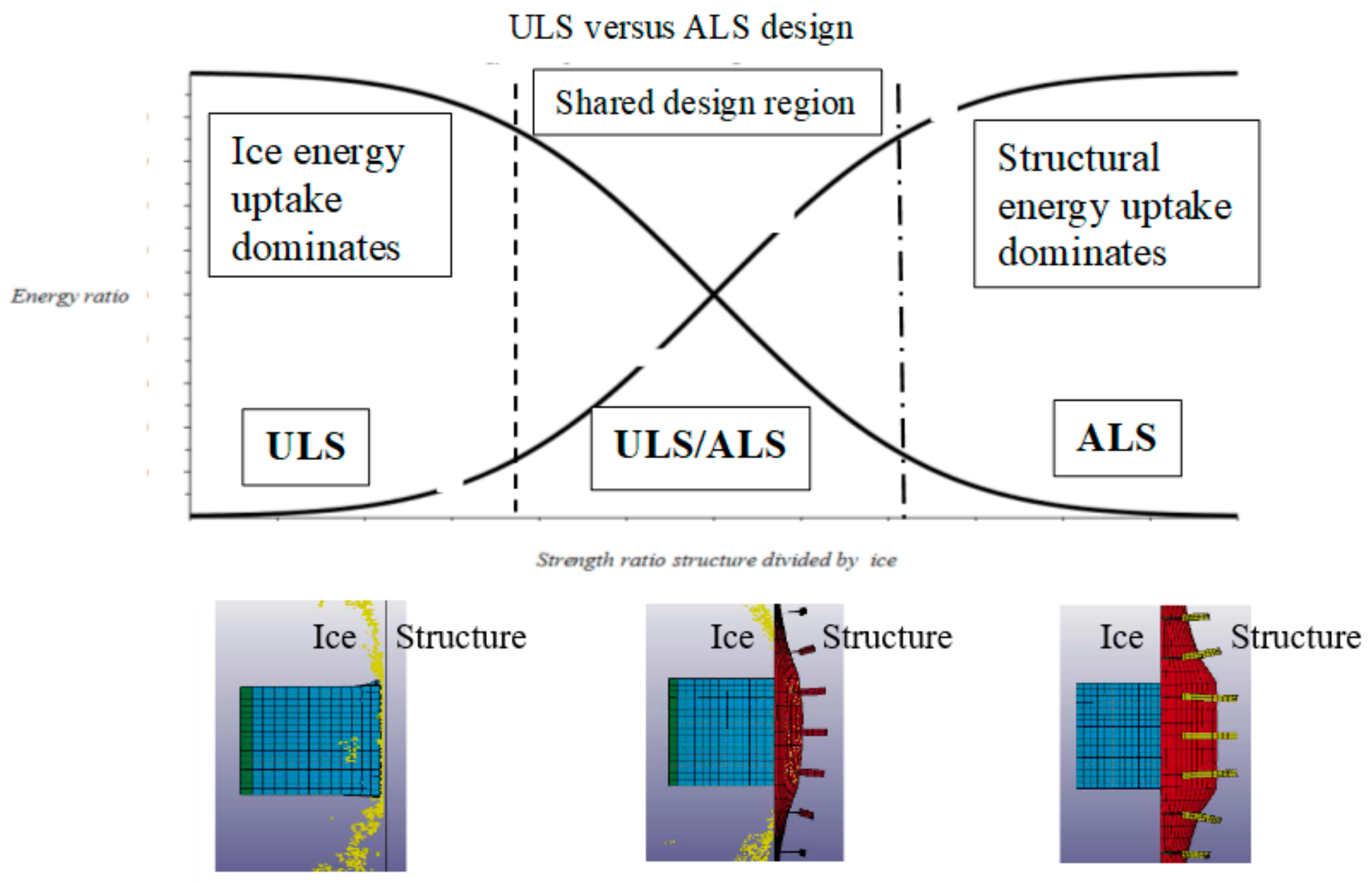
As discussed above, the “permissible” structural damage is very different for the Ultimate versus the Accidental Limit State. This is thoroughly discussed, e.g., in [4,7,10]. A further illustration is provided by Figure 1, where relative ULS deformations are exemplified to the left and ALS deformations to the right. It is seen that the deformation of the ice is strongly influenced by the structural strength and the corresponding structural behavior.

The relative uptake of energy by the ice feature versus the structure is shown in the lower part of the figure—for the ULS design the impact energy is mainly absorbed by the ice feature, while for the ALS design the structure typically absorbs most of the total kinetic energy. This total kinetic energy for the ship–ice system just prior to the impact event can be expressed as follows [10,16]:

$$E_S=\frac{1}{2}\left(m_s+a_s\right)v_s^2\frac{{\left(1-\frac{v_i}{v_s}\right)}^2}{1+\left(\frac{m_s+a_s}{m_i+a_i}\right)}$$

(1)

where m_s and a_s are the dry mass and the added mass of the ship (e.g., [17]), respectively; m_i and a_i denote the corresponding quantities for the ice feature; v_s is the corresponding speed of the ship, and v_i that of the ice feature.

The energy balance (by disregard remaining energy in the system after impact, e.g., due to the ship or the ice feature having nonzero velocities) is then expressed as the kinetic energy before the impact being equal to the sum of the energy absorbed by the structure and that absorbed by the ice feature:

E_s = E_s,ice + E_s,structure

(2)

where the first term represents the energy absorbed by the ice feature and the second term corresponds to the energy that is absorbed by the structure.

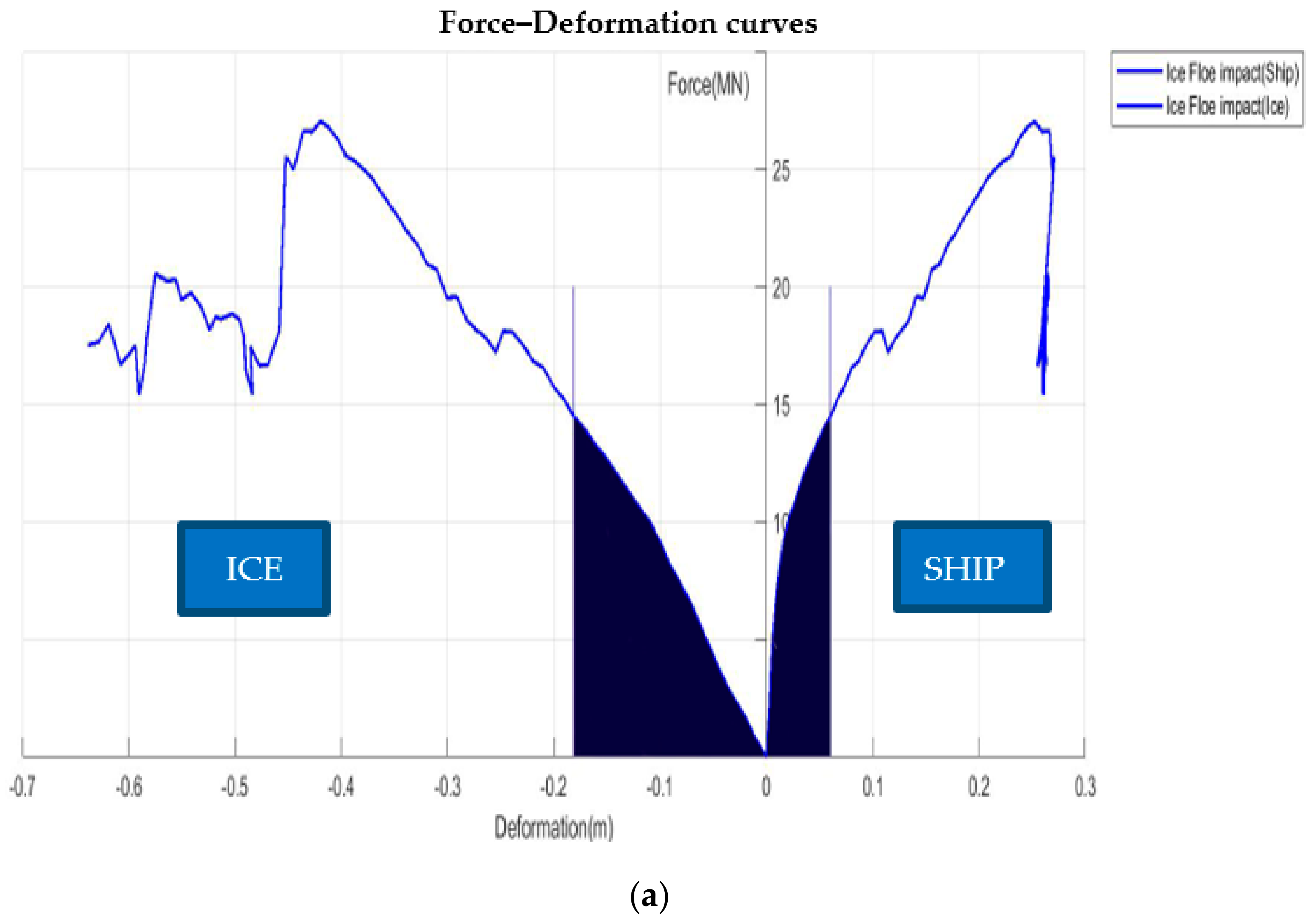
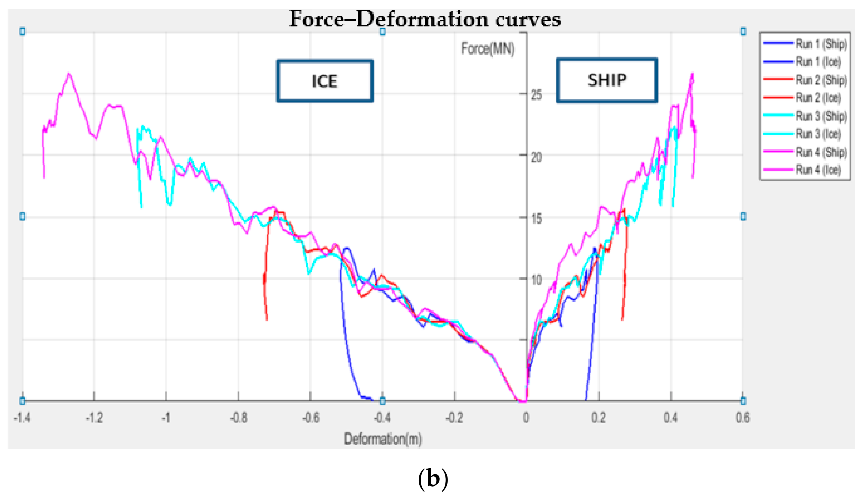
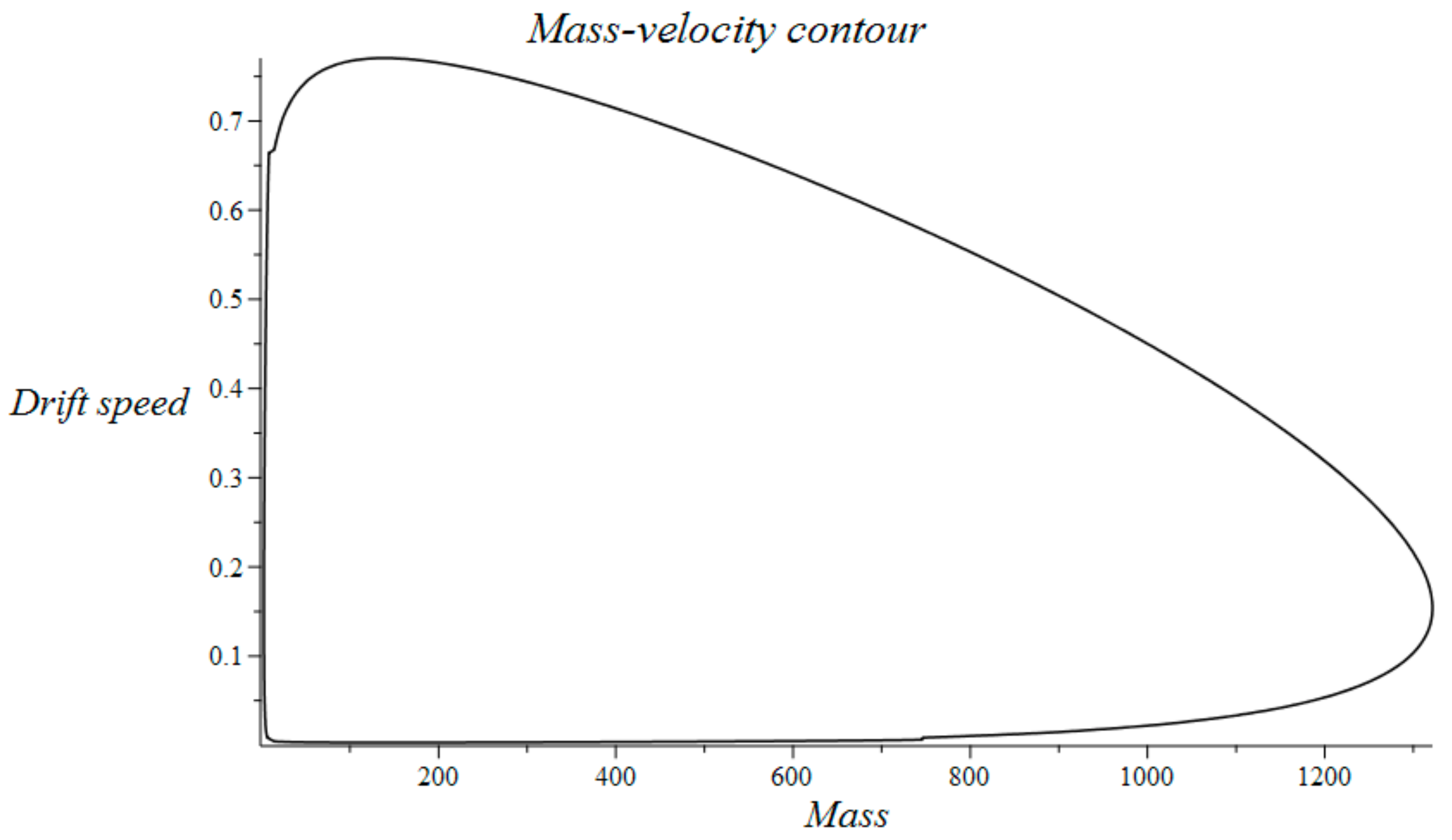
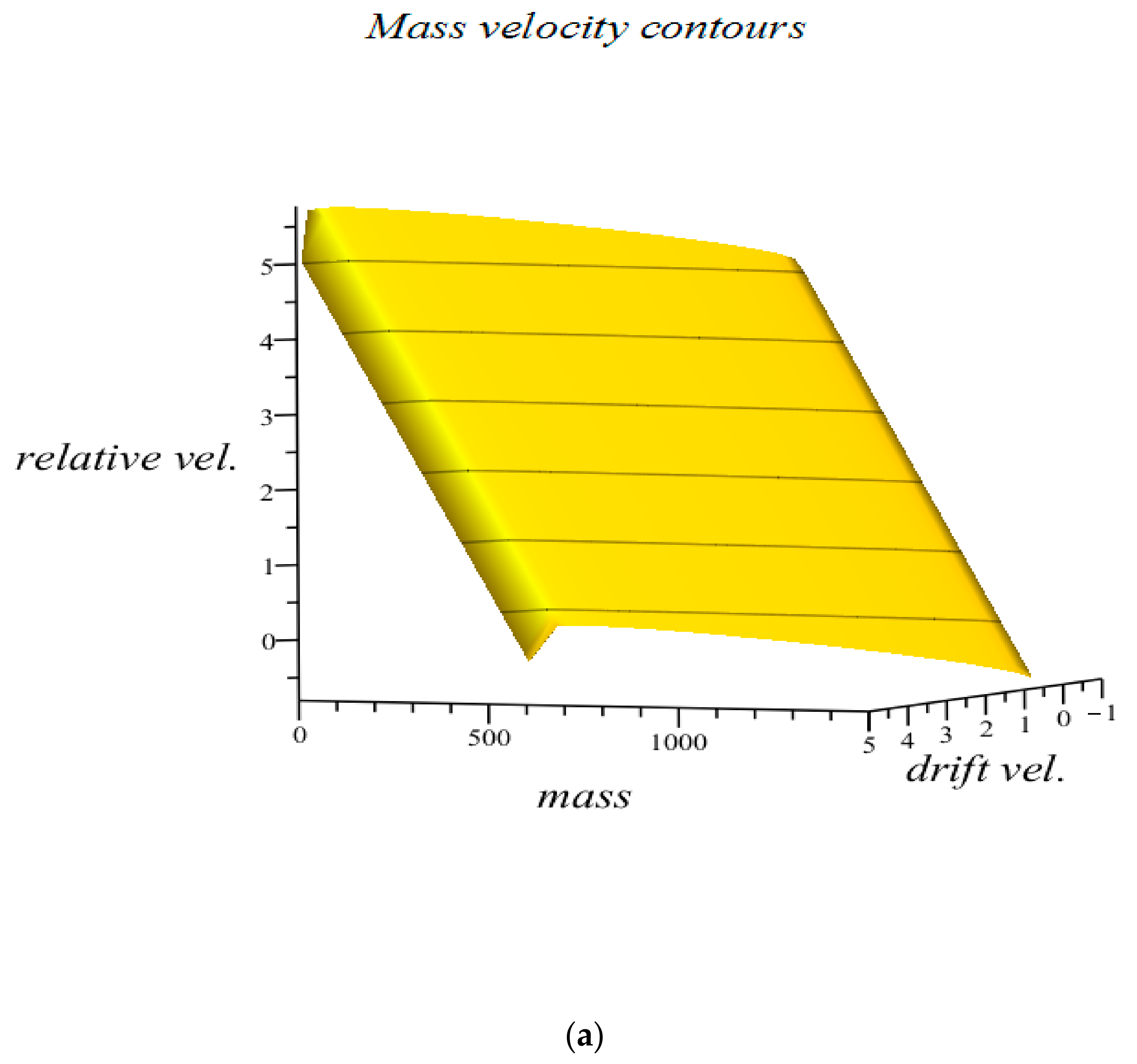
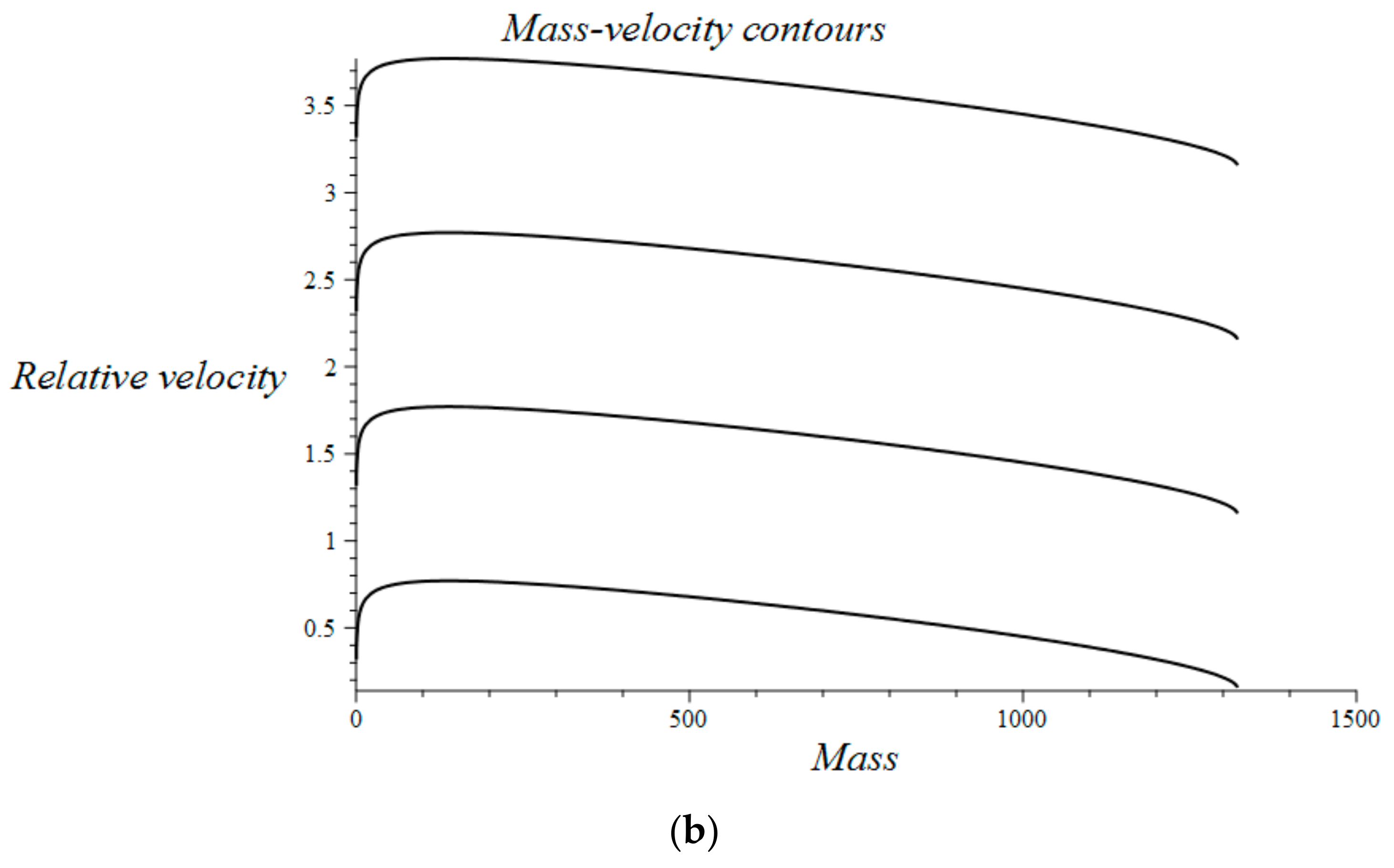
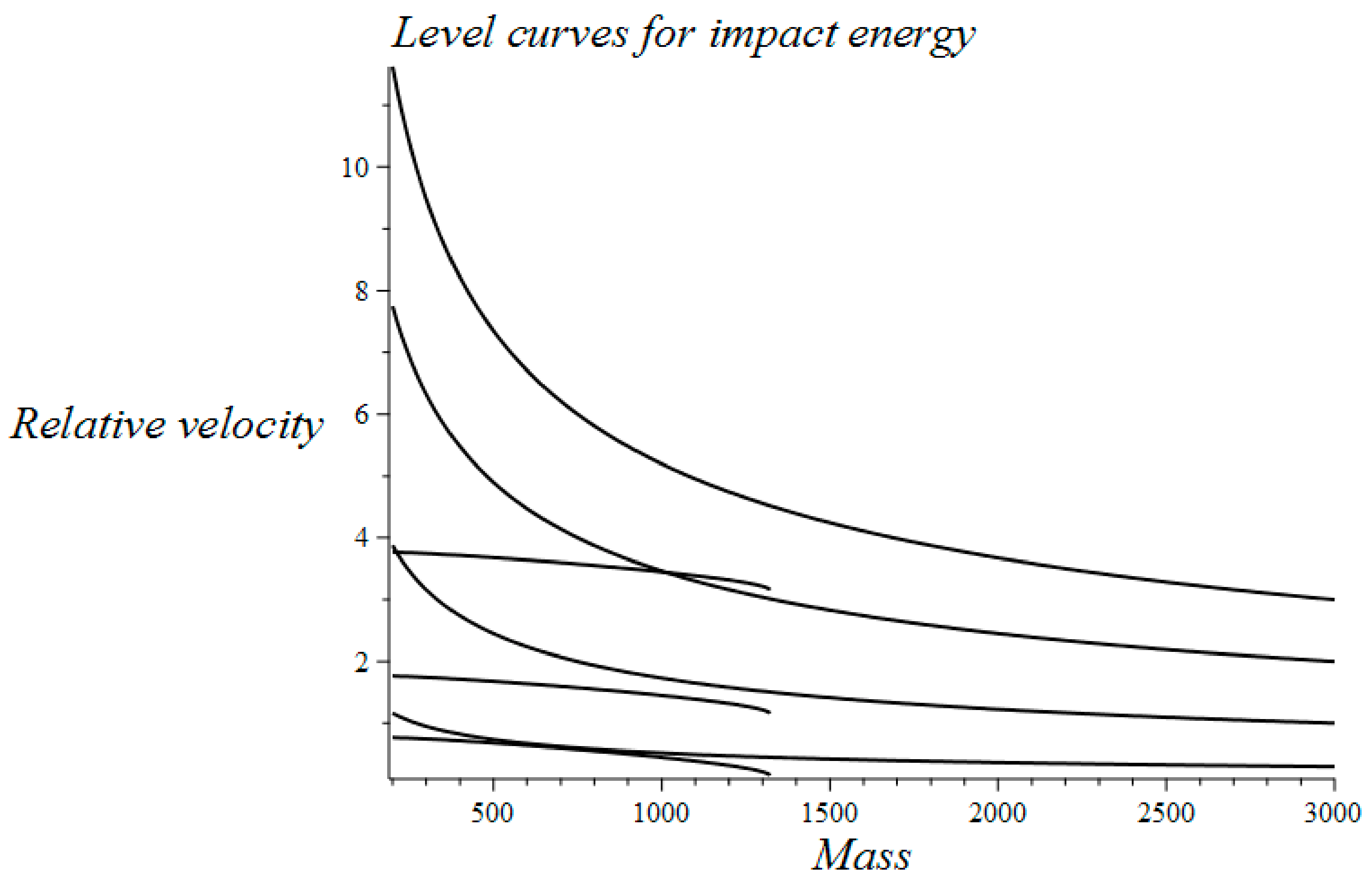
The absorbed energies correspond to the areas under the respective force–displacement curves. The energy uptake by the structure versus the ice feature is further illustrated in Figure 2 [18] where the results correspond to a shared energy scenario. In Figure 2a, the amount of energy absorbed in the case of an ice floe impact is shown with the ice contribution to the left and the structural contribution to the right (shaded areas). In Figure 2b, load–displacement curves corresponding to increasing mass of the ice feature are shown where the blue curve corresponds to the smallest mass (288 tons) and the violet curve corresponds to the largest mass (1500 tons). It is seen that the maximum deformation increases for both the structure and for the ice feature as the impacting mass increases. This implies a corresponding increase of the sum of the absorbed energies that are required in order to balance the initial kinetic energy. In addition to initial kinetic energy, it is found that the local shape of the ice feature for the part where the impact occurs also has a strong influence on the resulting contact force and relative amount of energy absorption.

3. Environmental Contour Method

The main idea behind design contours is to identify the most relevant environmental conditions corresponding to a specific return period (or equivalently specified in terms of a probability of exceedance). Subsequently, response analyses are performed for a subset of these conditions. This saves computation time as compared to a more systematic and more accurate long-term response analysis for which the whole range of possible environmental conditions must be considered.

In order to perform such a full long-term analysis, the following two-step procedure is relevant:

I. The ULS or ALS criterion is first expressed on the following form:

$$G\left(y_c,\mathit{S}\right)=y_c-Y\left(\mathit{S}\right)$$

(3)

Here, G(∙) designates the mechanical failure function; the n-dimensional vector S = (S₁, S₂, …, S_n)^T denotes the basic design variables for which the joint probability density function (PDF) is assumed to be known, which is denoted by f_S(s). Y(S) is the internal load effect in the structure. The quantity y_c is the corresponding design capacity (which can be a function of several deterministic parameters and/or additional random variables related to the structural properties). Typically, the load effect and structural capacity is formulated in terms of stresses, forces, and bending moments.

As an example in relation to the ULS, y_c may, e.g., correspond to the design value of the yield stress of the steel for the ship hull and Y(S) will then represent the maximum stress load effect in the hull (as a function of the values of the basic design variables). However, since this corresponds to a very strict design criterion, it is more relevant instead to take y_c to designate a maximum permissible plastic strain limit (which for a particular hull member can be translated into a maximum plastic deformation limit). The quantity Y(S) then designates the maximum strain load effect in the hull. Similarly for the ALS, y_c may refer to a critical plastic strain limit which generally is higher than for the ULS. Depending on the accidental scenario, it could even correspond to the fracture strain of the hull material or a certain maximum allowable fracture damage.

However, in the following, a formulation is also provided where both the load effect and capacity are defined in terms of energy levels, i.e., by applying the absorbed impact energy as the load effect and the critical impact energy (corresponding to a given failure mode) as the capacity. This is in accordance with the impact analysis approach outlined in the previous section.

II. The failure probability p_f of the structure corresponding to a given time in operation can next be calculated as:

$$p_f\left(y_c\right)={{\displaystyle \int }}_{G\left(y_c,\mathit{S}\right)\le 0}{f}_{\mathit{S}}\left(\mathit{s}\right)d\mathit{s}$$

(4)

Basically, this integral expresses the probability content that corresponds to the “volume” of the failure domain in the space which is spanned by the relevant random variables. The boundary of the failure domain is defined as the surface that is obtained by setting the mechanical limit state function in Equation (3) equal to zero.

The integral in Equation (4) can be only be expressed in closed form for cases where the joint PDF and the limit state function G(y_c, S) are given. However, this is quite rare in practice since the load effect Y(S) for a given value of the environmental parameter vector S usually needs to be obtained by means of numerical simulation and/or by experiments.

Evaluated of the integral can also be made by application of the Monte Carlo simulation technique (MCS) or by other reliability methods such as the first order or second order reliability methods (FORM/SORM) [19]. These approaches are based on the joint PDF and the failure surface G(y_c, S), which are combined in order to establish a transformation into a normalized space of independent, standard Gaussian variables (which is frequently referred to as the U-space). In the FORM approach, the failure surface in normalized space is represented by the tangent plane at the so-called design point. The corresponding probability of failure is approximated as:

$$p_f\left(y_c\right)\approx \mathsf{\Phi }\left(-\beta \right)$$

(5)

where Φ represents the standard normal cumulative distribution function (CDF); β denotes the reliability index, and this also corresponds to the distance between the design point to the origin in normalized space.

It is emphasized that the relationship between the failure probability and the standard cumulative Gaussian distribution function is due to the transformation into normalized and independent variables. Furthermore, this is a first order approximation based on linearization of the mechanical limit state function. Second order corrections to this approximation can be obtained, e.g., by the so-called SORM approximation. Generally, various types of Monte Carlo simulation techniques are also applied as a supplement to (or sometimes instead of) the approximation in Equation (5).

However, determination of the design load effect, y_N, which corresponds to the capacity that is required in order to withstand the loads associated with an N-year return period generally requires iterative reliability calculations for different values of y_c.

Accordingly, it is highly relevant to simplify Step II of the long-term analysis procedure, which is precisely the objective of environmental contour methods. The design contour for the N-year return period is frequently established by means of the inverse FORM (i.e., IFORM) approach [13,20]. The probability of failure, p_f(y_N) is then first specified in order to generate the environmental contour that corresponds to that probability. An n-dimensional sphere with the radius β_F, which is obtained by means of the specified failure probability as expressed by Equation (6), is then first created in the normalized Gaussian space:

$${\beta }_F={\mathsf{\Phi }}^{-1}(1-p_f(y_N))$$

(6)

This sphere is subsequently transformed into the physical parameter space to yield the design contour. The mapping can, e.g., be based on the inverse Rosenblatt transformation for cases where the joint density function of the variables is formulated by means of the conditional modelling approach [21] or by the Nataf transformation if the marginal PDFs of variables and the correlation coefficients between these variables are given [12]. The environmental contour obtained by the IFORM is accordingly the collection of physical environmental parameters that correspond to the normalized values, which are located on the sphere with radius β_F in the U space.

It is found that the main benefit of the design contour method is due to the description of the environmental parameters being uncoupled from computation of the structural response. Due to its high efficiency and satisfactory accuracy, the environmental contour method has, e.g., been widely applied for assessment of ULS criteria, and in particular during preliminary design phases. The most critical response corresponding to the environmental conditions defined by the environmental contour can then be applied for estimation of the extreme response for the specified return period. If the response process for a given ice condition is stochastic, the extreme response can be taken to be an upper fractile of the corresponding short-term extreme response distribution. This is similar to the approach applied in the case of wave-induced response [11].

4. First-Year Ice Ridges

4.1. Properties of Sea Ice Ridges

Sea ice that has survived one or more summers is referred to as old ice or multiyear ice. Typically, the relevant mechanical properties are then stronger than those corresponding to first-year sea ice [22]. It is pointed out in [23] that old ice could be encountered by Arctic ships and accordingly poses a threat to the ships. However, in the present study, only first-year sea ice ridges are considered. For one thing, the physical and mechanical properties of the first-year ice have been studied rather extensively, while very limited information is available with respect to old ice. The mechanical properties are assumed to be close to those of the surrounding level ice. Furthermore, most of the old ice is found at very high latitudes and the ice conditions, e.g., for the typical NSR are mostly first-year. Ice ridges are regarded as one of the major hazards that need to be considered for Arctic shipping routes. Ice ridge is a line or wall of broken ice components that are forced upwards due to shear or pressure. At an early stage, the ice ridges are formed as broken ice rubble. These blocks may subsequently to some extent become consolidated at the refreezing stage. As illustrated in Figure 2, there are generally three distinct parts in a first-year ridge [3]: the above-water sail part, the consolidated layer, and the ice rubble. The sail part has pores filled with air and snow. The consolidated layer forms the upper part of the ridge keel and is a continuous layer of ice. The ice blocks found in the lower part of the keel are loose and only partially refrozen. Due to the buoyancy forces, these rubble blocks are packed together with water being trapped between the blocks. Figure 3 gives an illustration of some of the key parameters that can characterize the geometry of a first-year ridge.

4.2. Ship–Ridge Interaction

A number of studies related to the interaction between ships and level ice, and ships and ice floes have been performed, e.g., [25,26,27,28]. However, there are few studies related to ship–ridge interaction, which is most likely due the complexity of such interaction processes. There are basically three different methods for prediction of structural loads caused by ridges, i.e., analytical (or semi-analytical) methods, numerical simulation models, and experimental tests. For the analytical and semi-analytical methods, the ship and ice interaction model is much simplified and well-suited for fast calculations. As an example, the loads caused by the sail can be neglected because its size is small compared to that of the keel [3]. Ice forces acting on ship-shaped structures can be divided into main load components–those caused by the consolidated layer part versus ones caused by the rubble blocks. Generally, the consolidated layer is 2.0–2.5 times thicker than the surrounding level ice. Furthermore, the mechanical properties of the consolidated layer are assumed to be close to those of the surrounding level ice. Therefore, the consolidated layer part can be considered as a thick level ice and the corresponding load components acting on fixed structures can be estimated by application of relevant formulas recommended in ISO 19906. For the load component caused by the rubble blocks, another empirical formula based on a passive mode of failure is also found in the same document.

In numerical simulation models, the consolidated layer and the rubble are in many cases modeled respectively as a thick level ice and a granular material. A number of numerical studies have been performed to study the interaction between a ship and level ice. An example is the three degree-of-freedom (3DOF) rigid model developed in [27]. This model has later been extended to comprise six degrees-of-freedom (6DOF) by Tan et al. [28]. Other studies are, e.g., those based on the finite element method (FEM), the graphics processing unit (GPU) computation basis [2,29], and the cohesive element method (CEM) [30]. In order to study the interaction between ice rubble and ships, numerical methods such as the DEM [31,32] and the FEM [33] have been applied. However, due to the complexity of the ice ridge and ship interaction process, little work has been carried out in relation to numerical simulation of the entire process where the simultaneous loading caused by both of the two different keel components have been accounted for.

Improved understanding of ridge breaking processes can be achieved by means of scaled model tests and field tests, but only results from a limited number of such studies are available. Model tests related to interaction between ships and ice ridges were, e.g., performed in the Hamburg Ship Model Basin (HSVA) [34]. The ridge sail as well as the keel (including both a consolidated layer and ice rubble) were represented. A ship can break through a ridge either in a continuous manner or by means of ramming. The type of interaction depends on the ridge breaking energy, and the propulsive and the kinetic energy of the ship. Model tests that were carried out at HSVA for a moored floater having a sloping surface have confirmed that ridge ice loads are significantly higher than the loads due to the adjacent level ice [35]. Field experiments related to ship hulls interacting with first-year ridges have also been reported, e.g., [36,37,38].

Based on the abovementioned studies of first-year ice ridges interacting with ships and sloping structures, the ship and ridge interaction process is illustrated in Figure 4. During early design stages, loading due to the ridge sail part can be neglected. Furthermore, ice loads due to the underwater keel can be divided into two parts: the component caused by the consolidated layer and the component due to the unconsolidated ice rubbles. Ice loads from the consolidated layer part are assumed to correspond to that due to thick level ice. The ship and level ice interaction process is generally initiated by a localized crushing of the ice edge. Subsequently, the contact area and the crushing force will increase when the ship penetrates the ice feature. The ice sheet eventually deforms out of its plane, and the resulting bending stresses induce a flexural failure at a certain distance away from the region where crushing occurs [5]. The rubble can be broken by means of the kinetic and propulsive ship hull energy, and by the broken parts of the consolidated layer. The local water current may also serve to clear the rubble and the broken ice pieces from the keel.

4.3. Statistical Models for Key Parameters Associated with Ice Ridges

The description of the ship–ridge interaction process given above gives reason to select four variables for characterization of ice ridges, and these also form the basis for establishment of environmental design contours. These four variables are the thickness of the consolidated layer, its crushing strength, its flexural strength, and the draft of the keel. Statistical models are introduced for each of these variables.

The thickness of the consolidated layer depends on geographical area, its environmental conditions, and the time of the season. Here, the consolidated layer thickness of ridges located in the Barents Sea is considered. The data sets for the thickness of the consolidated layer were collected from field measurements that were carried out from 2002 to 2011 [24]. Based on a statistical analysis, the Gamma distribution is found to provide a satisfactory description of the experimental data. The Gamma probability density function is given by:

$$f\left(h_{cl}\right)=\frac{1}{\mathsf{\Gamma }\left(k\right){\theta }^k}{h}_{cl}^{k-1}exp(-\frac{h_{cl}}{\theta })$$

(7)

where Γ(·) represents the gamma function, and θ and k are the scale and the shape parameters, respectively. The resulting values of the two parameters are found to be 2.97 (shape) and 0.54 (scale) based on application of the moment estimators. Fitting of a Gamma distribution to the data is illustrated in Figure 5 [39].

The distribution of the consolidated layer thickness will be different for different Polar regions, and also associated with large uncertainties. The data measured in the Barents Sea were obtained based on mechanical or thermal drilling, and these provide at least a certain amount of information. For other Polar regions, where only limited or lacking data coverage exists, utilization of data related to the thickness of the surrounding level ice can possibly provide an estimate of the distribution of the consolidated layer thickness by application of a representative “enhancement factor”.

Because there are very limited experimental data for the mechanical properties of the consolidated layer, these values are assumed to be close to those of the surrounding level ice due to limited experimental data for the consolidated layer of ice ridges. For the flexural strength of first-year sea ice, a large number of measurements have been performed in different Arctic regions [22]. This strength parameter depends basically on the ice temperature, salinity, and inherent brine volume. The data of flexural strength in the present study are based on those provided by Timco [40]. These comprise in situ experimental data obtained from different Arctic regions, such as Baffin Island, Greenland, and the Gulf of Bothnia, and the Canadian and Alaskan Beaufort Sea. The two-parameter Weibull distribution can typically be applied to describe probabilistic distribution of the flexural strength σ_f, which is expressed as:

$$f\left({\sigma }_f\right)=\frac{\beta }{\alpha }{\left(\frac{{\sigma }_f}{\alpha }\right)}^{\beta -1}exp\left(-{\left(\frac{{\sigma }_f}{\alpha }\right)}^{\beta }\right)$$

(8)

where the scale parameter α and the shape parameter β are determined as 0.582 and 2.090, respectively, by means of regression estimators as implemented in a probability paper. A fitted Weibull density function (PDF) for the flexural strength of first-year sea ice in the Arctic is shown in Figure 6 [39].

The level ice crushing strength depends on various parameters such as loading direction, porosity, salinity, temperature, failure mechanism, etc. For ship–ridge interaction, samples that are loaded in the horizontal direction should be considered. However, only limited data are published for such samples in relation to Arctic regions. An exception is the data from experiments in the Svalbard region and the Barents Sea. Based on experiments for the winter seasons during 2005–2012 [41,42], data from 363 horizontally loaded samples were collected. Based on a statistical analysis, it is found that the lognormal distribution, given by Equation (9), can provide a satisfactory description of the measurements.

$$f\left({\sigma }_c\right)=\frac{1}{\sqrt{2\pi }\sigma \cdot {\sigma }_c}exp(-\frac{{(ln{\sigma }_c-\mu )}^2}{2{\sigma }^2})$$

(9)

Here, σ_c represents the crushing strength of the ice feature, while μ = 0.644 and σ = 0.550 are, respectively, the mean value and the standard deviation (of the logarithmic values).

The fitted lognormal density function and histograms of the measured data are shown in Figure 7 [39]. It should be noted that the present probabilistic model for the crushing strength is based on the measured samples from the Barents Sea and Svalbard regions. This model can also be applied for representation of the distribution of crushing strength for first-year sea ice in other Arctic regions, but relevant data and experiments from other regions are also required in order to enrich the current probabilistic model.

Ridge loads acting on ship hulls due to the rubble blocks depend on the keel draft, the keel width, the keel porosity, and the mass of the keel part. Among these parameters, the draft of the keel h_k is the most prominent. This quantity depends on geographical location and time of the season, similar to the consolidated layer thickness, e.g., Samardžija and Høyland [43].

The magnitudes of the draft of the keel can be obtained by means of drilling or by performing continuous scanning. Data for the keel draft of first-year ridges in Arctic regions such as the Barents Sea, the Greenland area, and the Beaufort Sea, which are subjected to statistical analysis, form the basis for the present study. These data sets are published in [5], and they are mainly collected by mechanical and thermal drilling. It is observed that the exponential model with a PDF expressed as follows can give an adequate fit to the measurements [44]:

$$f\left(h_k\right)=\lambda exp\left(-\lambda \left(h_k-c\right)\right)$$

(10)

Here, h_k denotes the draft of the keel and λ is the parameter of the exponential model. The constant c can be regarded as a lower threshold (i.e., a “cut-off value”) for the keel draft.

When the data are obtained from a collection of different Polar regions, however, the three-parameter Weibull model given by Equation (11) is found to provide a better fit to the collective data sets than what can be achieved by means of the exponential distribution:

$$f\left(h_k\right)=\frac{\beta }{\alpha }{\left(\frac{h_k-c}{\alpha }\right)}^{\beta -1}exp\left(-{\left(\frac{h_k-c}{\alpha }\right)}^{\beta }\right)$$

(11)

Here, the scale parameter is estimated as α = 9.464, the shape parameter β is estimated as 1.697, and the location parameter is estimated as c = 0.450, based on application of the least square method.

Note that seasonal variations of the parameters that are applied for characterization of ice ridges have presently not been considered. Recent studies of such effects can be found, e.g., in [43,45,46].

5. Environmental Design Contours for Ice Ridges

The key ice ridge parameters and the associated probabilistic models pertaining to these parameters are described above. Based on these probabilistic models and the IFORM approach, various categories of environmental contours can be developed. This comprises two-dimensional contour lines, three-dimensional contour surfaces, and four-dimensional manifolds. These can subsequently be employed within the context of deterministic or reliability-based design of ships in Polar waters. Different types of such environmental contours are discussed in this section.

5.1. Two-Dimensional Contours

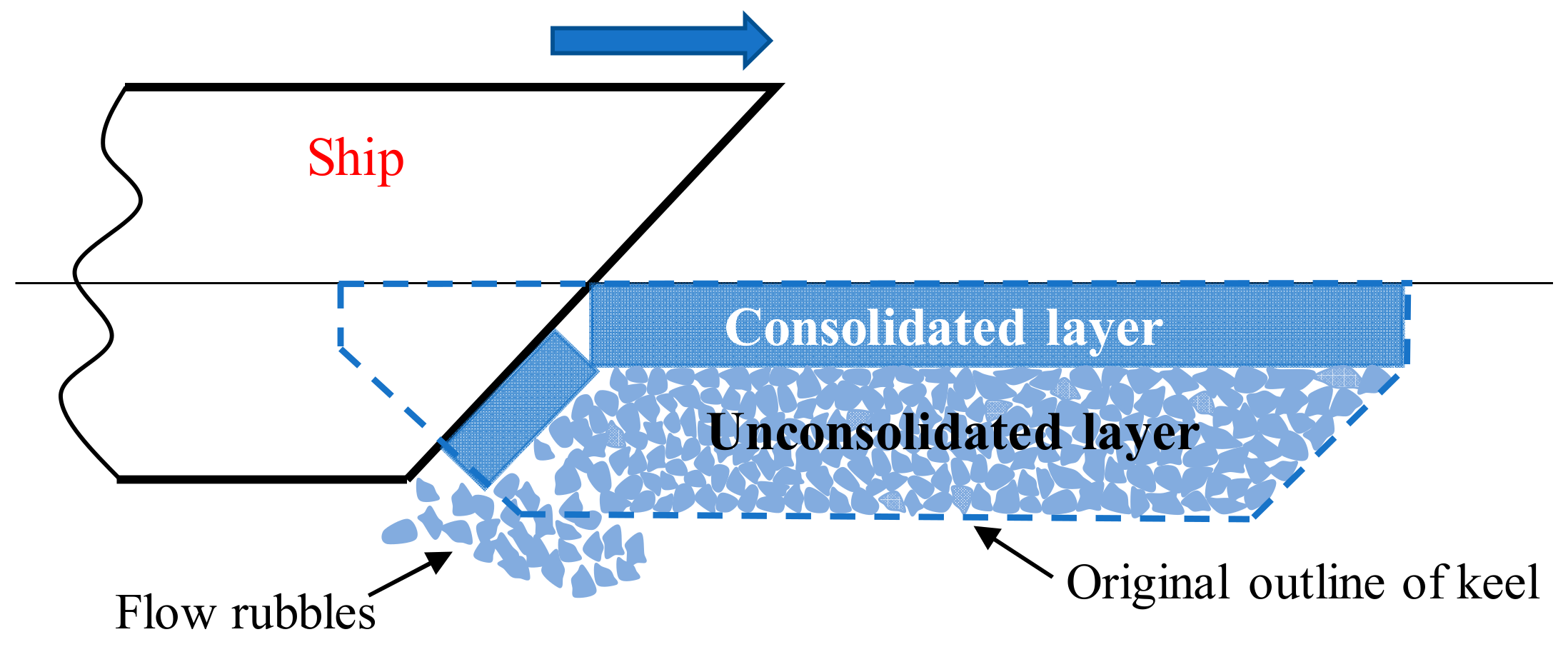
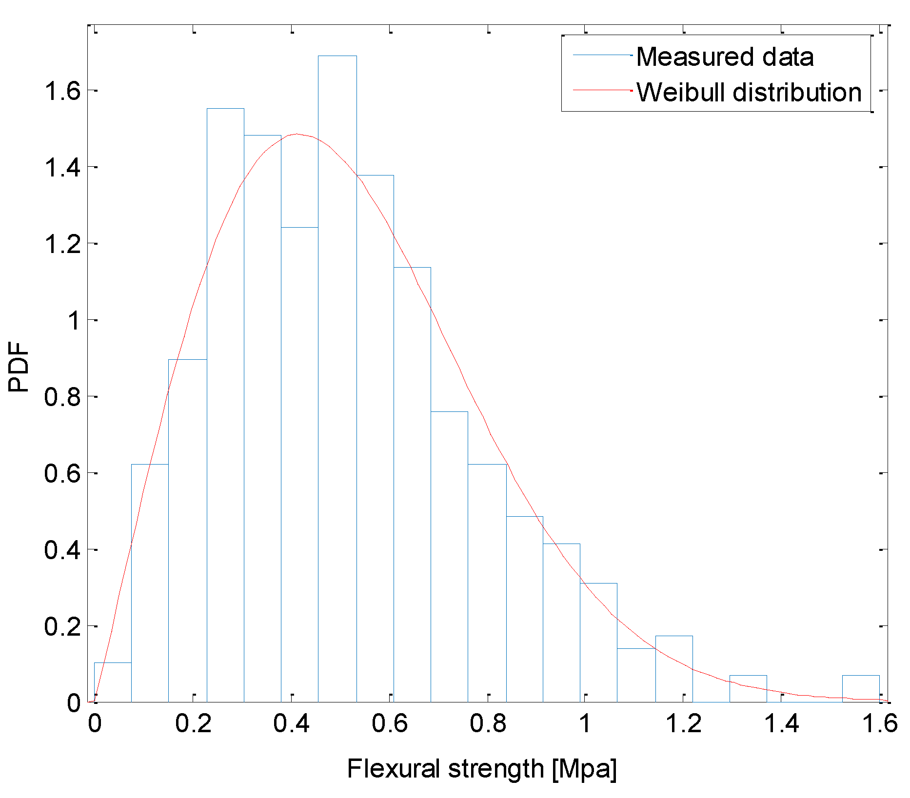
Among the three forms of environmental contours mentioned above, the environmental contour lines based on only two environmental parameters represent the simplest form. The ship–ridge interaction process can then be represented in a simplified manner as a sloping structure exposed to an incoming ice sheet. Ship-ice loads can accordingly be estimated by applying the empirical formula given in [3], which is used to calculate the static ice loads. This formula only requires the flexural strength and the consolidated layer thickness of the ice feature as input quantities. This simple model is clearly not completely satisfactory for representation of the ship–ice ridge interaction process, since both dynamic effects as well as ridge keel actions are not taken into account.

Still, such a model can be applied as a basis for illustration of the main steps associated with application of the design contours for estimation of the extreme ice ridge loads. Moreover, the effect of increasing correlation between the basic design parameters and an increasing number of encountered ice ridges corresponding to a given return period in relation to the resulting environmental contours can readily be investigated, which is due to the simplicity of the two-dimensional design contours.

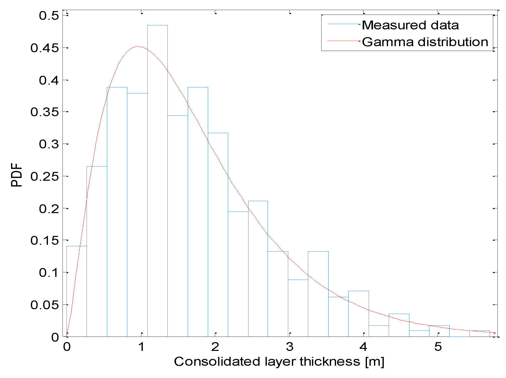
The specific location that is considered determines the probability distribution of the consolidated layer thickness. Presently, only experimental data that are collected for h_cl in the Barents Sea are available. Accordingly, it is assumed that the relevant Arctic ship mainly operates in the Barents Sea, and, furthermore, that it travels a distance of 5000 km per year in areas with ice ridges. The density of ice ridges is taken to be 2/km along the route [47]. The intended lifetime is assumed to be 50 years. Presently, ice conditions along the route are assumed to be constant during this period.

The annual number of ice ridges encountered by the ship is assumed to be a fixed value, which is given as N_1year = r∙5000 km∙2/km, where r is the encounter frequency that depends on the capability of the navigation equipment on board and the experience of the crew. The number of ridges experienced by the ship hull during the service life, N_50years, is then obtained:

$$N_{50years}=50\cdot N_{1year}=50\cdot r\cdot 5000\cdot 2$$

(12)

The radius of the circle in the normalized space, β_F, which corresponds to this return period is determined by:

$${\beta }_F={\Phi }^{-1}\left(1-p_f\left(y_N\right)\right)={\Phi }^{-1}\left(1-\frac{1}{N_{50years}}\right)$$

(13)

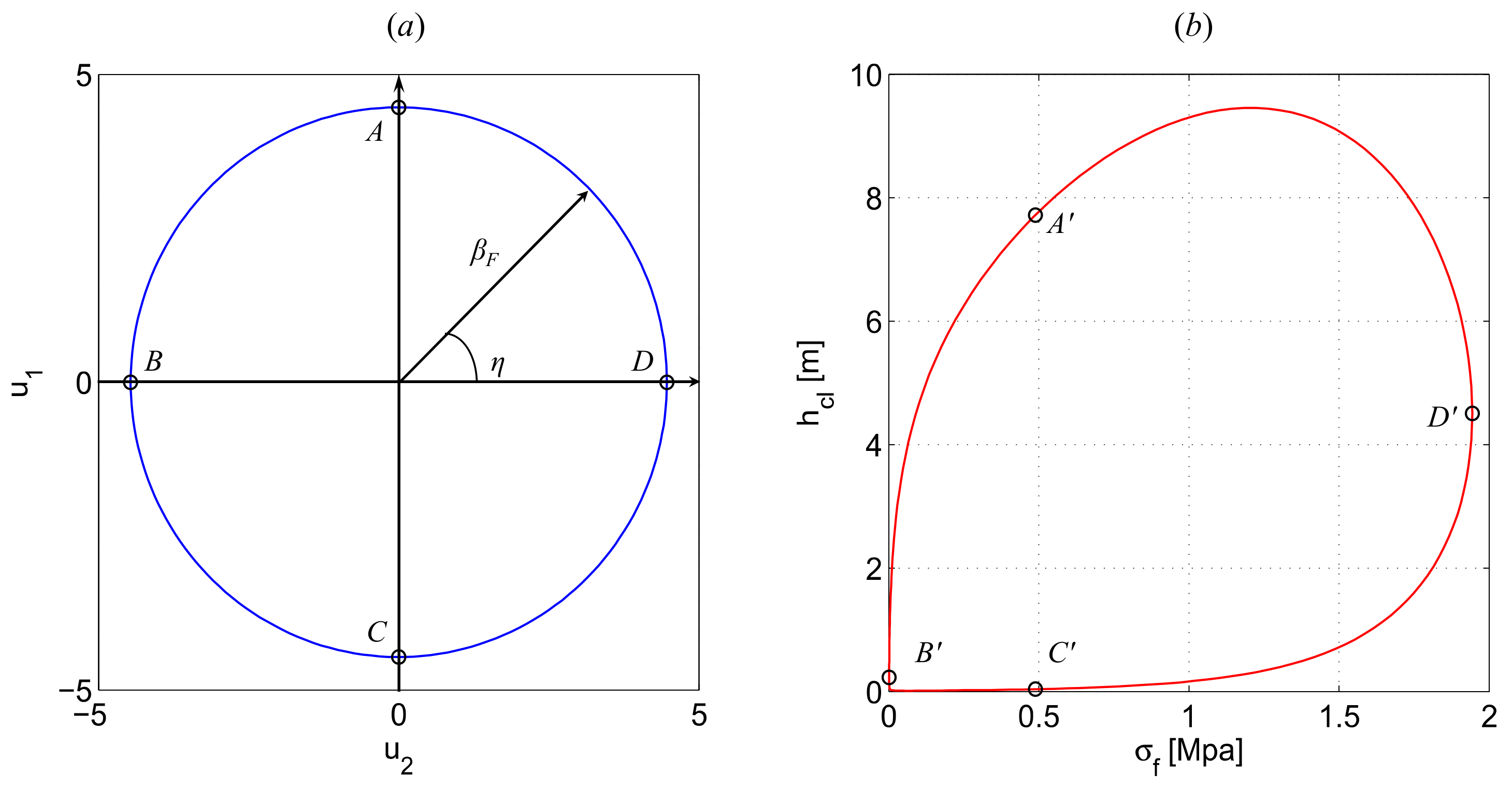
A circle corresponding to r = 0.5 (which gives N_50years = 250,000) is plotted in Figure 8a, where u₁ and u₂ are independent normalized Gaussian variables given by u₁ = β_F∙sin(η) and u₂ = β_F∙cos(η), where the angle η ranges between 0 and 2π.

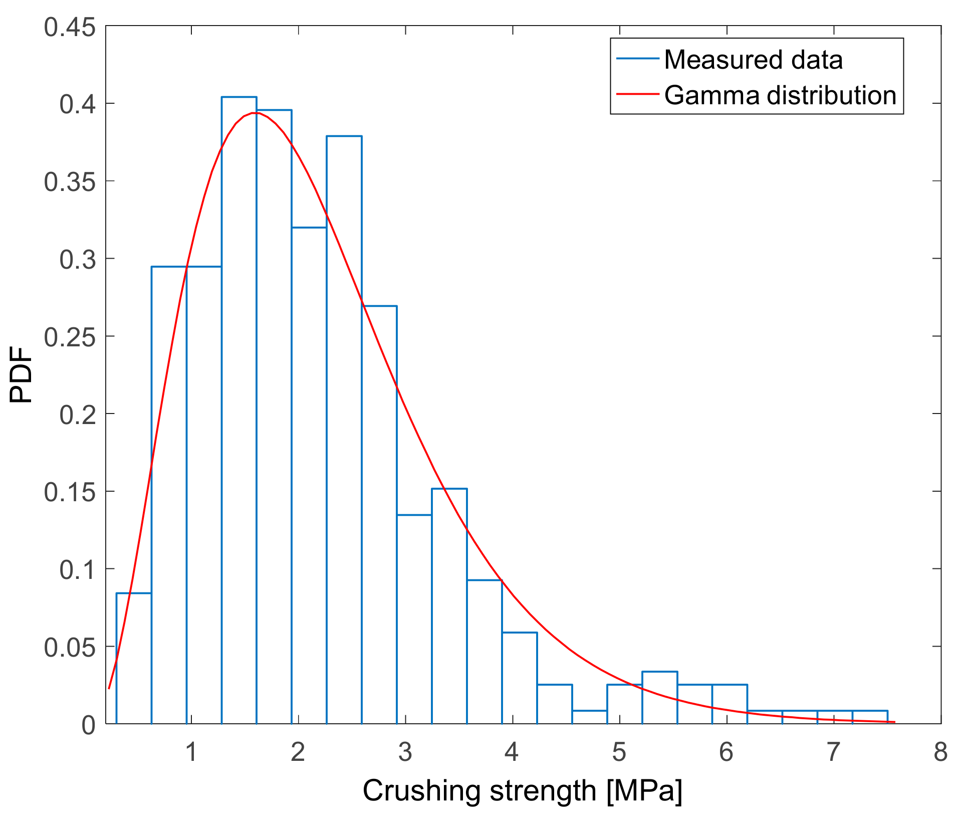
Presently, only the marginal PDFs of the key parameters are available, while the correlation coefficients between the two parameters are not known. The variables s₁ and s₂ are introduced, which correspond to the consolidated layer thickness and the ice crushing strength, respectively. The resulting design contour in physical parameter space is then established based on the circle in normalized space by application of the Nataf transformation, which is expressed as follows:

$$\begin{gathered} s_1=F_{S_1}^{-1}\left(\Phi \left(u_1\right)\right) \\ {s}_2=F_{S_2}^{-1}\left(\Phi \left(u_2\sqrt{1-{{\rho }^{\prime }}_{12}^2}+{\rho }_{12}^{\prime }{\Phi }^{-1}\left(F_{S_1}\left(s_1\right)\right)\right)\right) \end{gathered}$$

(14)

Here, ρ₁₂ denotes the correlation coefficient between the crushing strength and the thickness of the consolidated layer. This coefficient is related to ρ′_12, which denotes the associated (equivalent) coefficient of correlation that is applied by the Nataf transformation. The two correlation coefficients are connected by a semiempirical equation of the following type. The structural response corresponds to

$${\rho }_{12}^{\prime }=\zeta \cdot {\rho }_{12}$$

(15)

where relevant expressions for the function ζ can be found in [48].

The contour line for a 50-year return period is presented in Figure 8b for the case that the correlation coefficient ρ₁₂ is 0.5. In order to illustrate the result of the transformation into physical space, four points that are located on the circle in normalized space are selected. These are denoted by A, B, C, and D in the figure. The four points are then mapped into the corresponding points in the physical parameter space. These are designated by A′, B′, C′, and D′. Having generated the contour line corresponding to a 50-year return period, the associated extreme load level, y_N, can be estimated based on the following principle:

y_N ≈ maximum load around the (s₁, s₂) contour

(16)

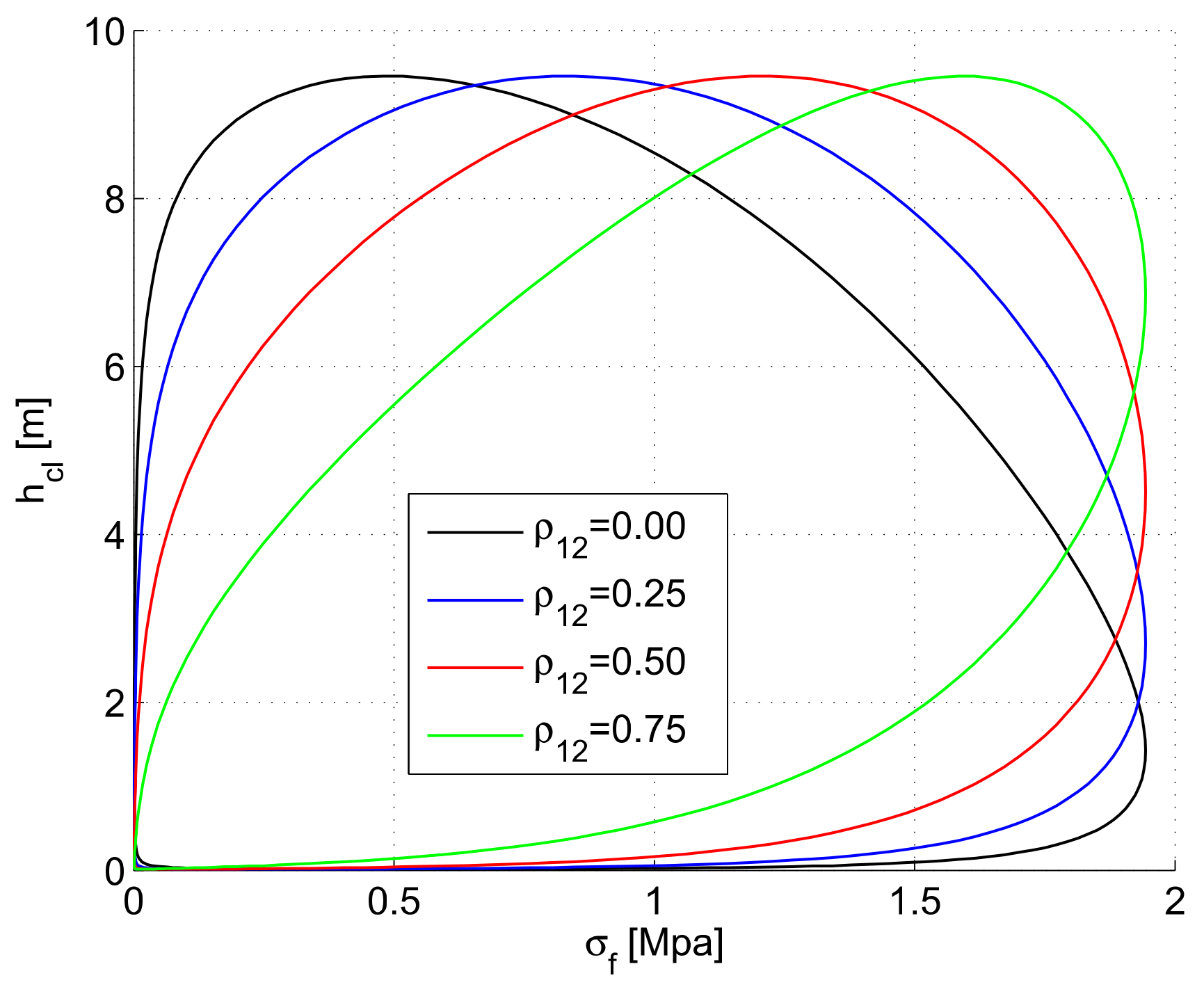
Accordingly, the extreme response/loads can be simplified by searching along the contour for the most critical environmental condition. The values of correlation coefficient ρ₁₂ and the encounter frequency r are selected somewhat arbitrarily due to the limitation of reference data. The influence of these two variables on the subsequent contour lines can be studied. For a given value of r, the effect of increasing the correlation coefficient ρ₁₂ on the environmental contour is first shown in Figure 9.

From this figure, it is seen that the shapes of the environmental contour lines are strongly influenced by the value of the correlation coefficient. There are no changes of the maximum values for the flexural strength and the consolidated layer thickness along the different contour lines for varying values of ρ₁₂. However, the critical region where the simultaneous values of the consolidated layer thickness and the flexural strength are high is seen to become increasingly narrow for increasing values of the correlation coefficient. This narrowing implies that high values of consolidated layer thickness have a stronger tendency to be associated with high values of flexural strength, and this generally implies more serious ice loads. Increasing values of the correlation coefficient will accordingly generally imply an increase of the maximum loads caused by the ice conditions along the contour line (which also implies an increase of the extreme hull response associated with a given return period).

The influence of encounter frequency r on the environmental contour is next studied for the case that the correlation coefficient has a specific value of 0.50. The contour lines corresponding to varying r values then have similar shapes since they are based on the same coefficient of correlation. Increased value of r implies that a higher number of load events are experienced by the ship hull for the same return period. The corresponding contour lines then expand accordingly. The maximum value along the thickness axis changes from 9 m to almost 10 m when r changes from 0.2 to 0.75. For the flexural strength, the maxim value changes from 1.8 MPa to almost 2 MPa. Clearly, this gives increasingly higher ridge loads as the encounter frequency increases.

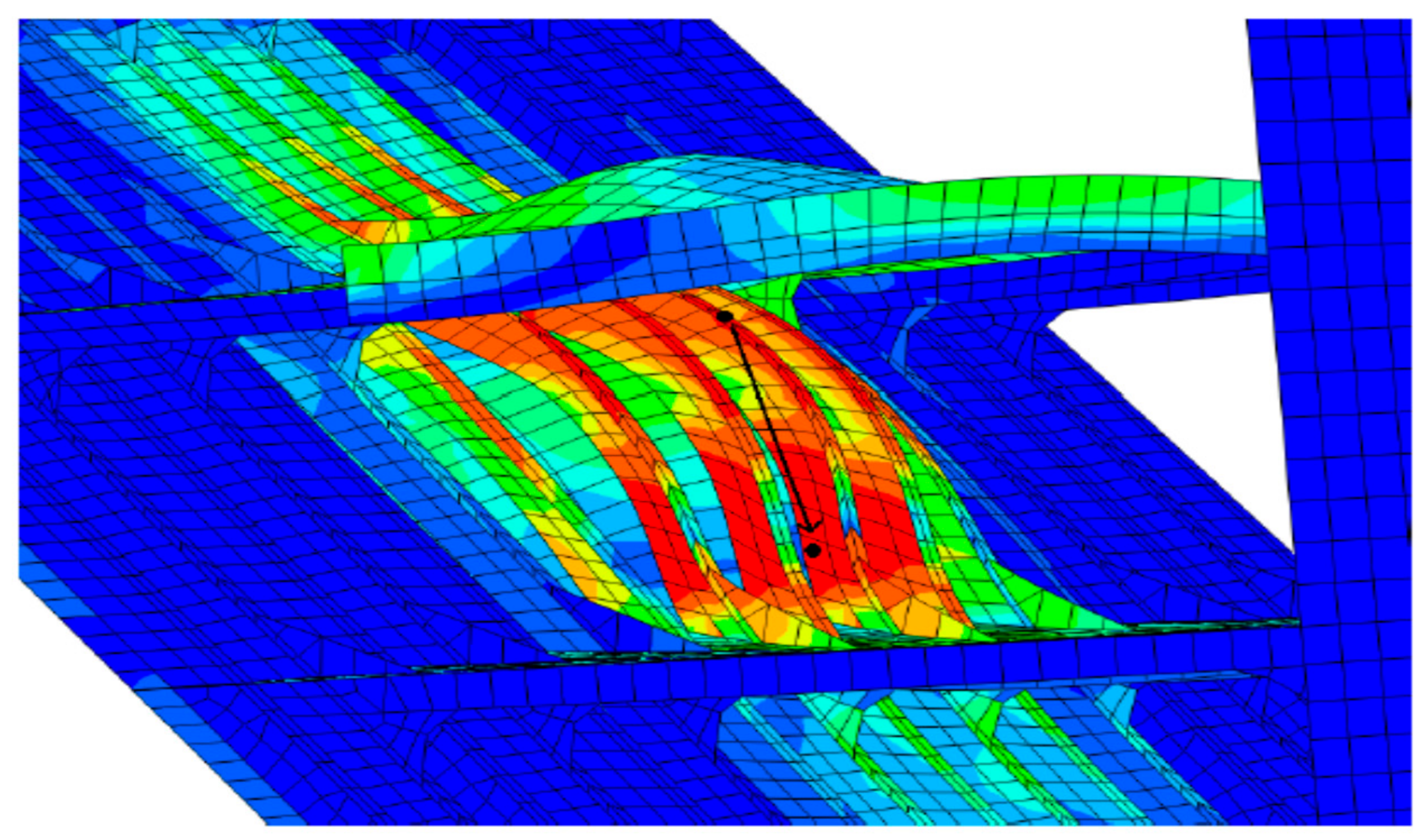
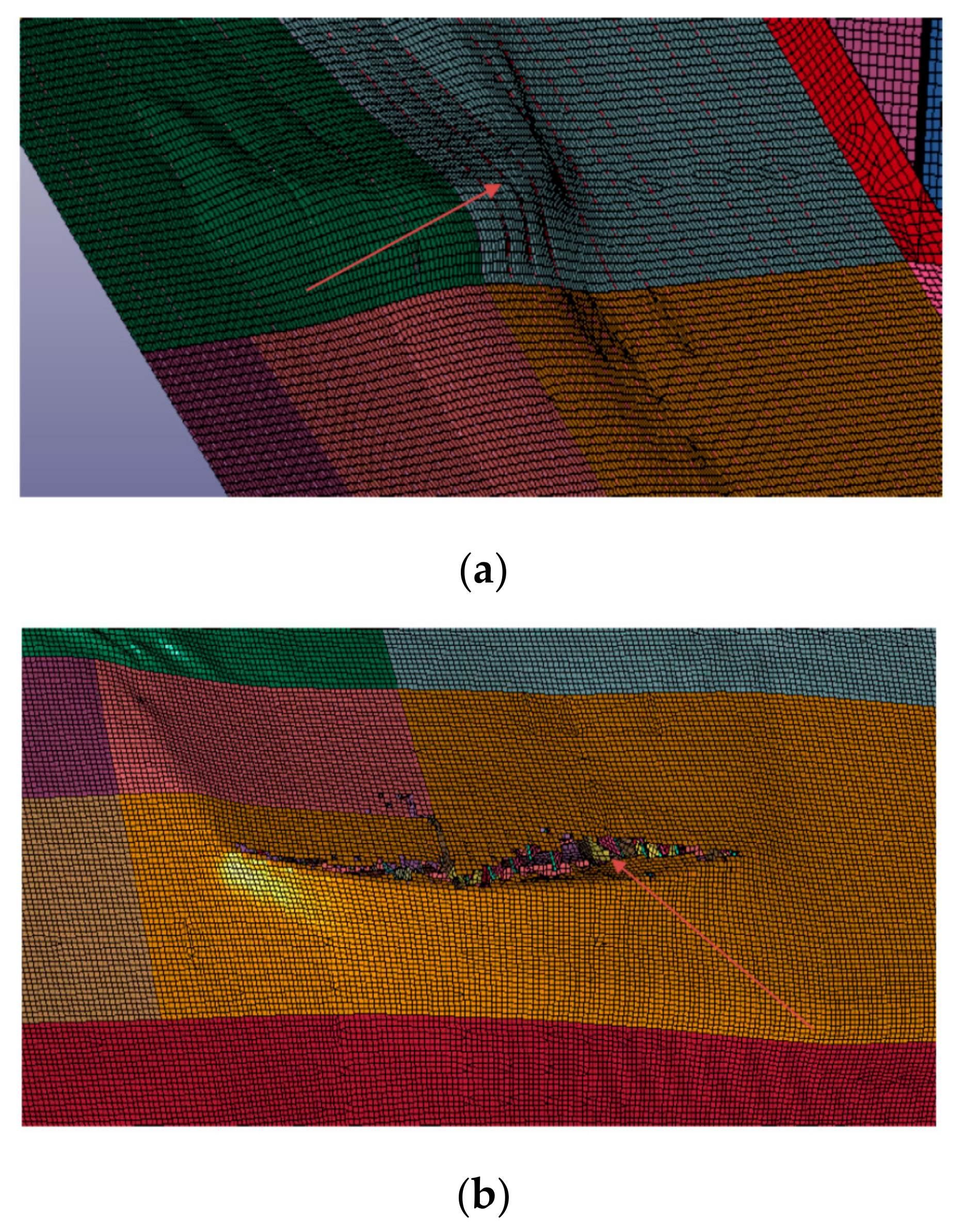
For stationary structures (e.g., floating production systems, FPSOs), the ridge encounter frequencies depend upon the arrival rate at the site where the structure is located. Accordingly, it cannot be influenced or controlled unless, e.g., disconnect systems or protective barriers are applied. An intermediate situation becomes relevant for floating units that are intended for temporary but extended operations, such as exploration, drilling, and installation vessels. An example of computed deformations and stresses caused by the impact of an ice ridge on the upward sloping hull of a mobile drilling unit (MODU) is shown in Figure 10 [49]. The structural response corresponds to permanent plastic deformations without any fracture taking place, and accordingly this would correspond to a mechanical limit state of the ULS/ALS category.

5.2. Three-Dimensional Contour Surfaces

In order to obtain more general types of ice-loads than those restricted to the two-parameter model proposed in Section 5.1, models with three parameters for characterization of the ice ridge properties can also readily be accommodated within the present approach. Two specific examples of three-parameter combinations are (i) layer thickness/crushing strength/flexural strength and (ii) layer thickness/keel draft/flexural strength. Both of these cases are considered in [39]. Here, only the first alternative is addressed.

For this model, possible load contributions caused by the unconsolidated rubble are excluded. The main ice loads caused by the ship and ridge interaction are now assumed to be dominated by the consolidated layer part [14]. However, dynamic effects associated with the ship–ice interaction process can be included as part of numerical simulations or relevant empirical or theoretical load formulations. Accordingly, the consolidated layer thickness, the flexural strength, and the crushing strength are included as the relevant parameters. As compared to the contour based on two variables, the third component s₃ represents the ice ridge crushing strength. The corresponding variable u₃ in the normalized U space is also now expressed by means of the Nataf model based on introduction of two additional equivalent correlation coefficients (i.e., ρ′₁₃ and ρ′₂₃):

$$\begin{array}{c}{s}_1=F_{S_1}^{-1}\left(\Phi \left(u_1\right)\right)\\ s_2=F_{S_2}^{-1}\left(\Phi \left(u_2\sqrt{1-{{\rho }^{\prime }}_{12}^2}+{\rho }_{12}^{\prime }{\Phi }^{-1}\left(F_{S_1}\left(s_1\right)\right)\right)\right)\\ s_3=F_{S_3}^{-1}(\Phi (\frac{u_3}{\sqrt{1-{{\rho }^{\prime }}_{12}^2}}\sqrt{1-{{\rho }^{\prime }}_{12}^2-{{\rho }^{\prime }}_{13}^2-{{\rho }^{\prime }}_{23}^2+2{\rho }_{12}^{\prime }{\rho }_{13}^{\prime }{\rho }_{23}^{\prime }}\\ +\frac{1}{1-{{\rho }^{\prime }}_{12}^2}\left(\left({\rho }_{13}^{\prime }-{\rho }_{12}^{\prime }{\rho }_{23}^{\prime }\right){\Phi }^{-1}\left(F_{S_1}\left(s_1\right)\right)+\left({\rho }_{23}^{\prime }-{\rho }_{12}^{\prime }{\rho }_{13}^{\prime }\right){\Phi }^{-1}\left(F_{S_2}\left(s_2\right)\right)\right)\end{array}$$

(17)

where the quantities ρ′_ij (i, j = 1, 2, 3; i ≠ j) designate equivalent correlation coefficients that are applied by the Nataf transformation.

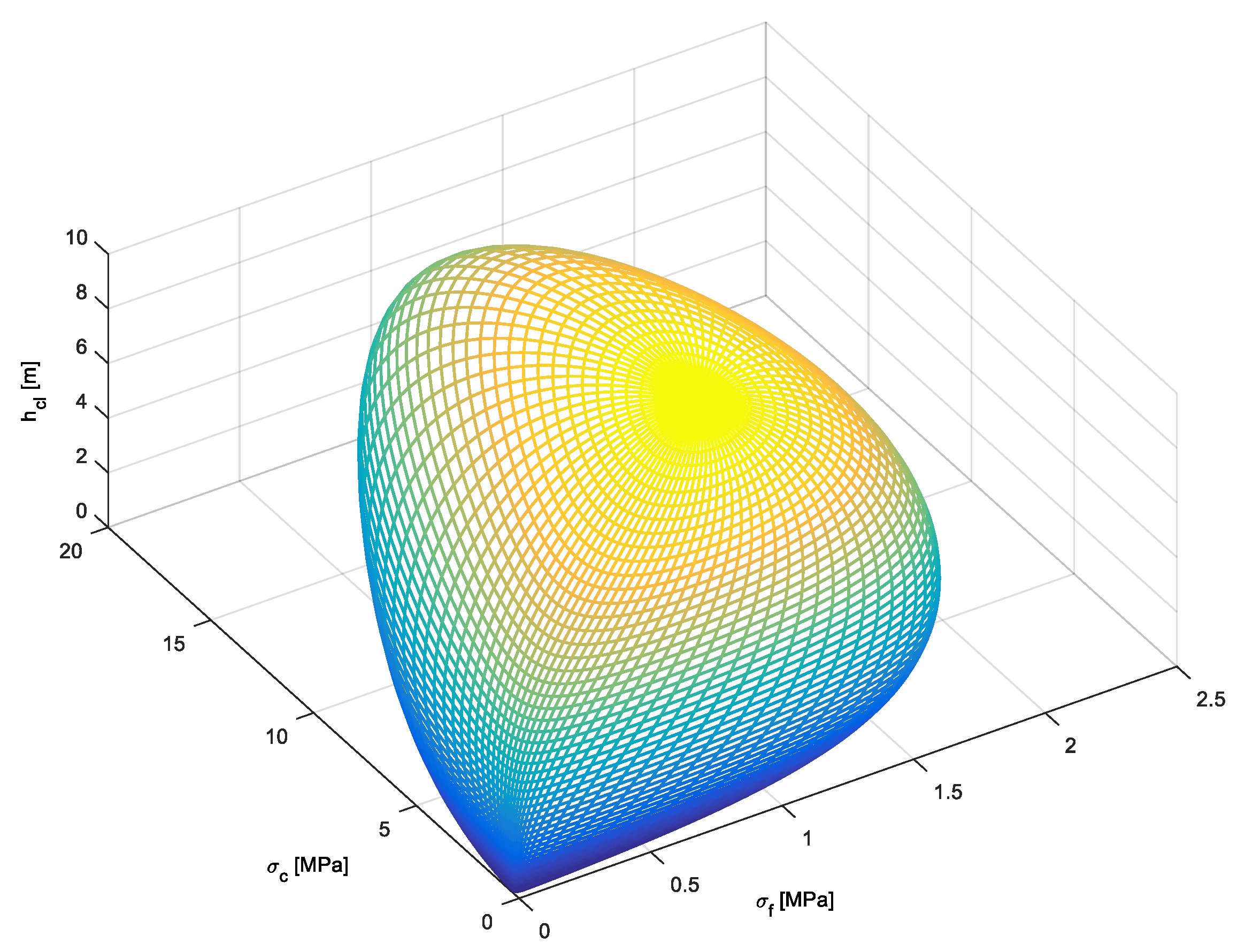
As an example, a case is considered for which all the three correlation coefficients in the joint statistical mode are equal to 0.5. The encounter frequency r is assumed to be 0.5 and the parameters of the statistical models are set to be the same as those described above. As an extension of the two-dimensional contours, a sphere with radius β_F in three dimensions is next established in the normalized space. A three-dimensional design contour in the physical parameter space is subsequently obtained by means of a transformation based on the Nataf model according to Equation (17). The resulting contour surface with three key parameters, i.e., the consolidated layer thickness, the flexural strength, and the crushing strength (corresponding to a return period of 50 years) is plotted in Figure 11 [39].

To provide a detailed visualization of the contour surface, a suite of contour lines in two dimensions, which are established by locking the value of one of the parameters (e.g., the consolidated layer thickness), could have also been constructed.

Having established the contour surface that corresponds to the three basic parameters selected, a set of ice ridge conditions that correspond to specific joint values of these parameters can be selected. These conditions correspond to specific points located on the contour surface. For each of these points, a “response analysis” is performed, e.g., by means of numerical calculations, empirical expressions, analytical solutions, and/or experimental tests. The most critical ice ridge condition is then subsequently identified. This yields an estimate of the highest ice ridge load and allows calculation of the associated extreme 50-year hull response.

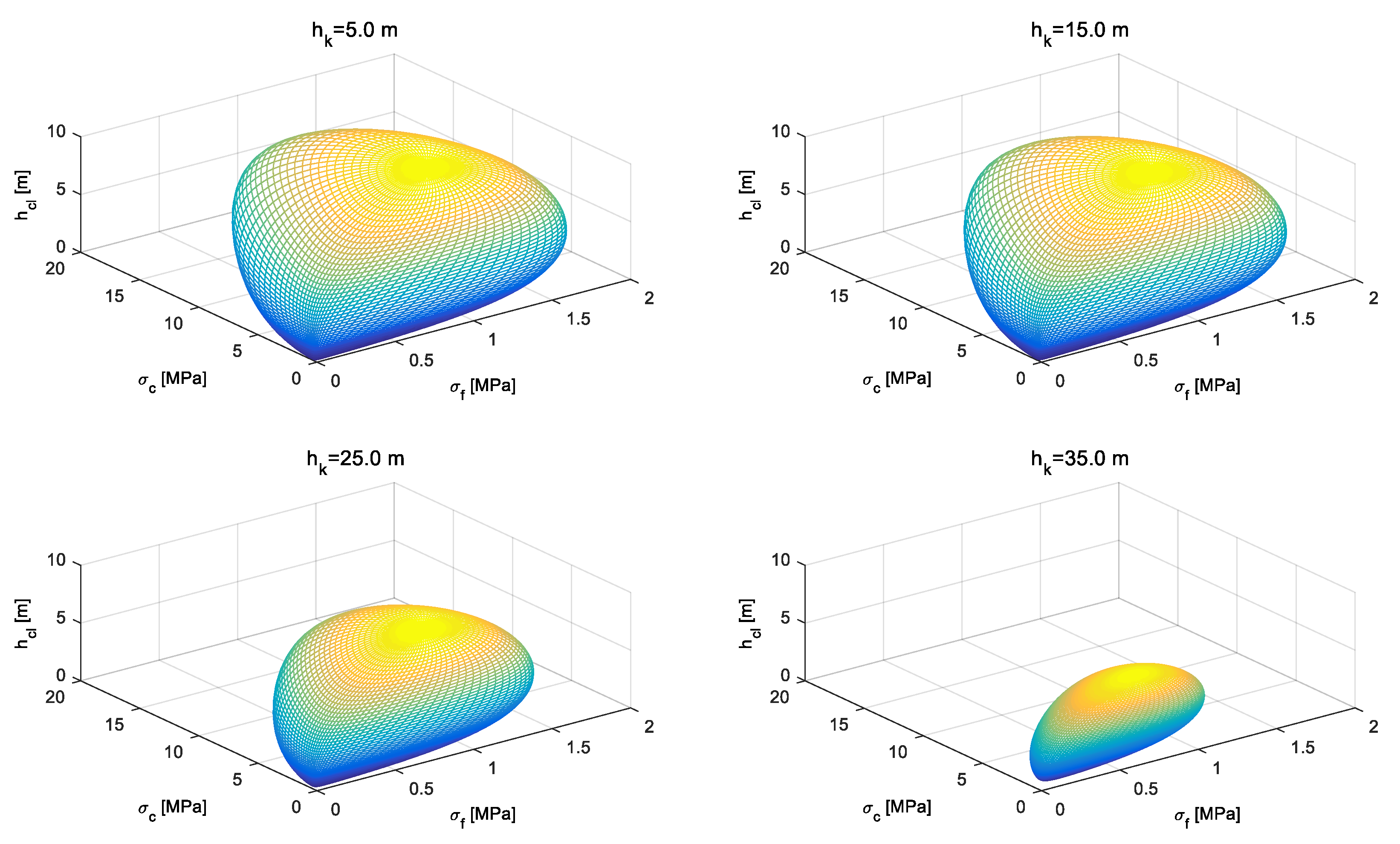
5.3. Environmental Contour for the Case with Four Parameters

Although the model just discussed with three basic ice ridge parameters is more comprehensive than the model with only two parameters, it may still not be adequate for some design purposes. As an example, the possible contribution to the ice loading caused by the unconsolidated rubble blocks is not considered. Accordingly, an even more refined four-parameter model, which also includes the keel draft as an additional random variable, can be relevant. Based on such a statistical representation, both the dynamic effects associated with the interaction between the consolidated layer and the ship hull, and the load effects due to the rubble blocks can be taken into account.

It is relevant to assume that there is no correlation between the keel draft and the other three key parameters. The other coefficients of correlation ρ_ij (with i, j = 1, 2, 3; and i ≠ j) are hence set equal to 0.5 for the purpose of illustrating the resulting contour. The other parameters, such as r and N_50years, are kept the same as for the example calculations above. For the purpose of visualizing the four-parameter contour (for a return period of 50 years), a set of environmental contour surfaces which correspond to specific values of the keel draft are displayed in Figure 12.

For a specific keel draft, the equivalent value of u₄ in normalized space is obtained by applying the transformation given by Equation (17). Then, a sphere of radius β_F (given in Equation (13)) is established in the normalized space of three standard Gaussian variables u₁, u₂, and u_3. This three-dimensional sphere is subsequently transformed into the space of physical parameters that results in the contour surfaces shown in Figure 12. The surfaces that correspond to different values of h_k are of a similar shape due to identical correlation relationships with respect to the four basic parameters. It is also seen that for keel drafts above the mean value (h_k = 8.89 m), the volume that is bounded by the contour surface decreases for increasing values of the draft. Having established such a set of contour surfaces associated with the return period of 50 years, the next task is for the designer to find the ice ridge conditions that are located on the surface (for a given draft), which cause the highest response levels in the ship hull. This requires consideration of a range of keel drafts, which adds some effort for identifying the most critical ridge characteristics, as compared to the case with only three parameters.

6. Design Contours for Growlers, Bergy Bits, and Icebergs

6.1. General

There are two mainly different populations of ice features of this type: (i) Growlers and bergy bits with water lengths of the order of 0–5 m and 5–20 m, respectively. The corresponding mass intervals are from 0 to 1000 tons for growlers and from 1000 tons to 10,000 tons for bergy bits, according to Raghuvanshi and Ehlers (2015). (ii) Icebergs classified are into small icebergs from 10,000 tons to 100,000 tons, medium icebergs from 100,000 tons to 1,000,000 tons (1 million tons), and large icebergs from 1,000,000 tons and greater [50].

The probability distribution for the mass corresponding to each of the populations is assumed to be of the exponential type. According to Fuglem et al. [51], the mass of both populations can be related to the waterline length according to the following formula:

M_Iceberg = 0.3 L_w³ (length in m and mass in tons)

(18)

A somewhat more refined formula involving the dimensions along the three orthogonal directions is given in [50].

6.2. Two-Dimensional Design Contours

The PDF for the water line length proposed in [51] is expressed as:

$$f_{Lw}\left(x\right)=0.43\left(\frac{1}{60}{e}^{-\frac{x}{60}}\right)+0.57\left(\frac{1}{8}{e}^{-\frac{x}{8}}\right)$$

(19)

This is due to the hypothesis that the number of icebergs with L greater than 20 m should approximately be equal to the number of icebergs with waterline length between 5 and 20 m. In the following, this probability model is applied for the purpose of illustrating the construction of two-dimensional environmental contours by also including the iceberg drift velocity as a random variable.

Data of ice drift speed in the Pechora Sea were collected by Løset and Onshus [48]. They found that a two-parameter Weibull distribution gave an adequate fit to the measurements:

F_X(x) = 1 − exp{−(x/θ)^γ}

(20)

where the scale and shape parameters are obtained as θ = 0.213 and γ = 1.406, respectively.

The probability for a ship to experience an impact from an ice feature is assumed to be higher for the smallest ice features (growlers and bergy bits) versus larger icebergs (given that a geographical encounter with such an object has taken place). Denoting the occurrence rates for the two main categories of ice features by ρ₁ and ρ₂ (per traveled distance unit for the ship), and the corresponding conditional collision probabilities by p_coll1 and p_coll2, the numbers of impacts during a period of N_year are then obtained as follows (with subscript 1 denoting smaller ice features and subscript 2 referring to larger features):

$$\begin{gathered} N_1=p_{coll1}\cdot N_{year}\cdot {\rho }_1\cdot L \\ {N}_2=p_{coll2}\cdot N_{year}\cdot {\rho }_2\cdot L \end{gathered}$$

(21)

where L is the average distance traveled by the ship in Polar waters per year. The corresponding probabilities of exceedance and reliability indices are then obtained as:

$$\begin{gathered} P_{f1}=\frac{1}{N_1},{\beta }_{F1}={\Phi }^{-1}\left(1-P_{f1}\right) \\ {P}_{f2}=\frac{1}{N_1},{\beta }_{F2}={\Phi }^{-1}\left(1-P_{f2}\right) \end{gathered}$$

(22)

By application of the cumulative distribution for the mass of the ice feature and the cumulative distribution for the drift speed, the corresponding two-dimensional environmental design contour can be obtained (by also assuming that mass and drift speed are uncorrelated). It is reasonable to consider collision with the two main categories of ice features as two distinctly different events, since the induced structural damage level typically is significantly different. Accordingly, the cumulative distribution function for the mass is also split in two by application of the respective terms for the density function in Equation (19).

As an example, a case where the number of impact events for the growler/bergy bit category is N₁ = 750 is considered, which implies that the corresponding exceedance probability is 0.00135. This gives a circle with radius equal to three in the normalized plane, and the resulting mass–velocity contour in the physical parameter plane is shown in Figure 13.

By also including the ship speed as a deterministic parameter, a sequence of two-dimensional contours of a similar type is obtained. These are shown as a 3D surface in Figure 14a with the relative speed (ship speed plus drift speed) along the second horizontal axis, and the drift speed along the vertical axis. The corresponding 2D projections are illustrated in Figure 14b.

In order to identify the relevant design scenario in terms of ice feature mass and relative velocity, the level curves corresponding to constant kinetic energy are required. The corresponding tangent point between these level curves and the mass–velocity contours then represent the most critical scenario along the environmental contour. This is illustrated in Figure 15. It is seen that for increasing ship speeds, the tangent points are shifted towards increasingly greater values for the mass of the ice feature.

Examples of numerically simulated structural damage for this category of ice features are shown in Figure 16 [18]. In the left part, Figure 16a shows the damage level in terms of permanent plastic deformations that would correspond to ULS/ALS-type of design criteria. In the right part, Figure 16b illustrates a damage that resulted in fracture of the steel plating, and this would correspond to an ALS-type of criterion.

6.3. Inclusion of Additional Iceberg Collision Parameters

There are a number of additional parameters that influence the amount of energy absorbed by the ship hull. Examples include local shape of the ice feature in the impact area, collision angle, material properties of the ship hull, elevation, and longitudinal position of impact location.

Some of these parameters can be characterized as belonging to the so-called “external impact mechanics”, while others correspond to the “internal impact mechanics”, e.g., [10,52,53,54]. However, little information is available in relation to statistics for the parameters that characterize the ice impact scenarios themselves. Possibly, relevant information could be extracted from collision statistics related to ship–ship interactions, e.g., [55].

It is found that the local shape of the ice feature in the impact area has strong influence on the amount of energy that is absorbed by the ship hull. Some examples of numerical models that are applied in order to represent various types of ice features are shown in Figure 17 [18]. It will be possible to include a “shape peakedness factor” as part of an extended three-dimensional environmental ice contour. A uniform probability model can initially be applied for such a parameter unless more specific information becomes available.

7. Conclusions

In this work, based on the interaction processes between ships and ice ridges/icebergs, relevant parameters associated with these ice features for determining the loading on a ship hull are addressed. Probabilistic models are applied in order to describe the available data for key design parameters. The potential for application of environmental contours for analysis and design of ships in Polar regions is illustrated. By application of the inverse FORM method (IFORM), different categories of design contours are generated by reflecting the number of parameters associated with the process of ship–ice interaction.

The effect of increasing the correlation between the environmental parameters and the influence from the encounter frequency r on the resulting environmental contour are both studied. It is important that more research should be directed toward collecting data related to the degree of correlation among the physical/mechanical parameters of first-year sea ice since this has a strong effect on the design contour and on the extreme ice loads to which the ship hull is subjected.

The total number of ridge load events experienced by a Polar ship corresponding to a given return period is important for the resulting design load. The number of such events depends, e.g., on the frequency of encounter r, the annual travel distance, and the impact probability along the sailing route. In addition, global climate change also has some potential influence on the statistical characterization of the relevant parameters for the ice features considered. Such effects could be captured by a modified formulation of the proposed environmental contour method.

The data which form the basis for construction of the statistical models typically depend on area. Additional data for characterization of the level ice and the consolidated layer of ice ridges in other Polar areas are continuously being collected. Environmental contours for characterization of input parameters that are relevant for load and response calculations can accordingly be established also for these areas.

Furthermore, there is clearly a need for more explicit statistical information in relation to many of the other parameters that define relevant impact scenarios. As increasingly more empirical data become available, more accurate and refined design methods can be achieved.

This should also be seen in the light of recent design codes that move toward a more goal-based approach rather than the prescriptive rules of today [56,57,58]. This results in less specific details and less rigid design requirements. Design against accidental loads for ships in Polar regions must also take into account relevant ship operation criteria and corresponding transit restrictions for ships in Polar waters [59,60].

References

1. Bergström, M.; Leira, B.J.; Kujala, P. Future Scenarios for Arctic Shipping. In Proceedings of the Volume 7: Polar and Arctic Sciences and Technology; ASME International: Washington, DC, USA, 2020. [Google Scholar]
2. Hahn, M.; Dankowski, H.; Ehlers, S.; Erceg, S.; Rung, T.; Huisman, M.; Sjöblom, H.; Leira, B.J.; Chai, W. Numerical prediction of ship-ice interaction: A project presentation. In Proceedings of the 36th International Conference on Ocean, Offshore and Arctic Engineering, Trondheim, Norway, 25–30 June 2017. [Google Scholar]
3. ISO. ISO 19906: Petroleum and Natural Gas Industries–Arctic Offshore Structures; ISO: Geneva, Switzerland, 2010. [Google Scholar]
4. Ehlers, S.; Cheng, F.; Jordaan, I.; Kuehnlein, W.; Kujala, P.; Luo, Y.; Freeman, R.; Riska, K.; Sirkar, J.; Oh, Y.-T.; et al. Towards mission-based structural design for arctic regions. Ship Technol. Res. 2017, 64, 115–128. [Google Scholar] [CrossRef]
5. Chai, W.; Leira, B.J.; Naess, A. Probabilistic methods for estimation of the extreme value statistics of ship ice loads. Cold Reg. Sci. Technol. 2018, 146, 87–97. [Google Scholar] [CrossRef]
6. Lensu, M. Short Term Prediction of Ice Loads Experienced by Ice Going Ships; Helsinki University of Technology: Espoo, Finland, 2002. [Google Scholar]
7. Riska, K. On the Mechanics of the Ramming Interaction between a Ship and a Massive Ice Floe: Dissertation; VTT Technical Research Centre of Finland: Espoo, Finland, 1987. [Google Scholar]
8. Riska, K.; Bridges, R. Limit state design and methodologies in ice class rules for ships and standards for Arctic offshore structures. Mar. Struct. 2019, 63, 462–479. [Google Scholar] [CrossRef]
9. Leira, B.J. A comparison of stochastic process models for definition of design contours. Struct. Saf. 2008, 30, 493–505. [Google Scholar] [CrossRef]
10. Yu, Z.; Amdahl, J. A numerical solver for coupled dynamic simulation of glacial ice impacts considering hydrody-namic-ice-structure interaction. Ocean Eng. 2021, 226, 108827. [Google Scholar] [CrossRef]
11. DNV GL. Environmental Conditions and Environmental Loads (DNV-RP-C205); Det Norske Veritas AS: Oslo, Norway, 2014. [Google Scholar]
12. Silva-González, F.; Heredia-Zavoni, E.; Montes-Iturrizaga, R. Development of environmental contours using Nataf dis-tribution model. Ocean Eng. 2013, 58, 27–34. [Google Scholar] [CrossRef]
13. Winterstein, S.R.; Ude, T.C.; Cornell, C.A.; Bjerager, P.; Haver, S. Environmental parameters for extreme response: Inverse FORM with omission factors. In Proceedings of the ICOSSAR-93, Innsbruck, Austria, 9–13 August 1993; pp. 551–557. [Google Scholar]
14. Chai, W.; Leira, B.J. Environmental contours based on inverse SORM. Mar. Struct. 2018, 60, 34–51. [Google Scholar] [CrossRef] [Green Version]
15. Eckert-Gallup, A.C.; Sallaberry, C.J.; Dallman, A.R.; Neary, V.S. Application of principal component analysis (PCA) and improved joint probability distributions to the inverse first-order reliability method (I-FORM) for predicting extreme sea states. Ocean Eng. 2016, 112, 307–319. [Google Scholar] [CrossRef] [Green Version]
16. Lu, W.; Yu, Z.; Van den Berg, M.; Dennis, M.; Lubbad, R.; Hornnes, V.; Amdahl, J.; Løset, S.; Kim, E. Loads, Design and Operations of Floaters in the Arctic (Nord ST20). 2019. Available online: https://www.scinapse.io/papers/2905273220 (accessed on 21 June 2021).
17. Kim, S.J.; Korgersaar, M.; Ahmadi, N.; Taimuri, G.; Kujala, P.; Hirdaris, S. The influence of fluid structure interaction modelling on the dynamic response of ships subject to collision and grounding. Mar. Struct. 2021, 75, 102875. [Google Scholar] [CrossRef]
18. Radhakrishnan, G. Analysis of Accidental Iceberg Impacts with Large Passenger Vessels and FPSOs. Master’s Thesis, NTNU, Trondheim, Norway, Aalto University, Espoo, Finland, 2018. [Google Scholar]
19. Madsen, H.O.; Krenk, S.; Lind, N.C. Methods of Structural Safety; Courier Corporation: Chelmsford, MA, USA, 2006. [Google Scholar]
20. Haver, S.; Winterstein, S.R. Environmental contour lines: A method for estimating long term extremes by a short term analysis. Trans. Soc. Naval Archit. Mar. Eng. 2009, 116, 116–127. [Google Scholar]
21. Rosenblatt, M. Remarks on a Multivariate Transformation. Ann. Math. Stat. 1952, 23, 470–472. [Google Scholar] [CrossRef]
22. Timco, G.; Weeks, W. A review of the engineering properties of sea ice. Cold Reg. Sci. Technol. 2010, 60, 107–129. [Google Scholar] [CrossRef]
23. Shamaei, F.; Bergstrøm, M.; Li, F.; Taylor, R.; Kujula, P. Local pressures for ships in ice: Probabilistic analysis of full-scale line load data. Mar. Struct. 2020, 74, 102822. [Google Scholar] [CrossRef]
24. Strub-Klein, L.; Sudom, D. A comprehensive analysis of the morphology of first-year sea ice ridges. Cold Reg. Sci. Technol. 2012, 82, 94–109. [Google Scholar] [CrossRef]
25. Ni, B.-Y.; Chen, Z.-W.; Zhong, K.; Li, X.-A.; Xue, Y.-Z. Numerical Simulation of a Polar Ship Moving in Level Ice Based on a One-Way Coupling Method. J. Mar. Sci. Eng. 2020, 8, 692. [Google Scholar] [CrossRef]
26. Huang, L.; Tuhkuri, J.; Igrec, B.; Li, M.; Stagonas, D.; Toffoli, A.; Cardiff, P.; Thomas, G. Ship resistance when operating in floating ice floes: A combined CFD&DEM approach. Mar. Struct. 2020, 74, 102817. [Google Scholar] [CrossRef]
27. Su, B.; Riska, K.; Moan, T. A numerical method for the prediction of ship performance in level ice. Cold Reg. Sci. Technol. 2010, 60, 177–188. [Google Scholar] [CrossRef]
28. Tan, X.; Su, B.; Riska, K.; Moan, T. A six-degrees-of-freedom numerical model for level ice–ship interaction. Cold Reg. Sci. Technol. 2013, 92, 1–16. [Google Scholar] [CrossRef]
29. Huisman, M.; Janßen, C.F.; Rung, T.; Ehlers, S. Numerical simulation of ship-ice interactions with physics engines under consideration of ice breaking. In Proceedings of the 26th International Ocean and Polar Engineering Conference, Rhodes, Greece, 26 June–1 July 2016. [Google Scholar]
30. Lu, W.; Lubbad, R.; Løset, S. Simulating Ice-Sloping Structure Interactions with the Cohesive Element Method. J. Offshore Mech. Arct. Eng. 2014, 136, 031501. [Google Scholar] [CrossRef] [Green Version]
31. Ranta, J.; Polojärvi, A.; Tuhkuri, J. Ice loads on inclined marine structures—Virtual experiments on ice failure process evolution. Mar. Struct. 2018, 57, 72–86. [Google Scholar] [CrossRef]
32. Gong, H. Discrete-Element Modelling of Ship Interaction with Unconsolidated Ice Ridges: Ridge Resistance and Failure Be-Haviour. Ph.D. Thesis, Aalto University, Espoo, Finland, 2021. [Google Scholar]
33. Sand, B.; Horrigmoe, G. Simulations of ice ridge forces on conical structures. In Proceedings of the 8th International Offshore and Polar Engineering Conference, Montreal, QC, Canada, 24–29 May 1998. [Google Scholar]
34. Myland, D. Ships Breaking Through Sea Ice Ridges. Int. J. Offshore Polar Eng. 2014, 24, 28–34. [Google Scholar]
35. Dalane, O.; Aksnes, V.; Løset, S. A Moored Arctic Floater in First-Year Sea Ice Ridges. J. Offshore Mech. Arct. Eng. 2015, 137, 011501. [Google Scholar] [CrossRef]
36. Kujala, P. On the statistics of Ice Loads on Ship Hull in the Baltic; Helsinki University of Technology: Espoo, Finland, 1994. [Google Scholar]
37. Lemee, E.; Brown, T. Review of ridge failure against the confederation bridge. Cold Reg. Sci. Technol. 2005, 42, 1–15. [Google Scholar] [CrossRef]
38. Kuuliala, L.; Kujala, P.; Suominen, M.; Montewka, J. Estimating operability of ships in ridged ice fields. Cold Reg. Sci. Technol. 2017, 135, 51–61. [Google Scholar] [CrossRef]
39. Chai, W.; Leira, B.J.; Næss, A.; Høyland, K.V.; Ehlers, S. Development of Environmental Contours for Ice Ridge Statistics Applied to Reliability-Based Design of Arctic Ships. Struct. Saf. 2020, 87, 1019906. [Google Scholar] [CrossRef]
40. Timco, G.; O’Brien, S. Flexural strength equation for sea ice. Cold Reg. Sci. Technol. 1994, 22, 285–298. [Google Scholar] [CrossRef]
41. Bonath, V.; Patil, A.; Fransson, L.; Sand, B. Laboratory testing of compressive and tensile strength on level ice and ridged ice from Svalbard region. In Proceedings of the International Conference on Port and Ocean Engineering under Arctic Conditions, Espoo, Finland, 9–13 June 2013. [Google Scholar]
42. Strub-Klein, L. A Statistical Analysis of First-Year Level Ice Uniaxial Compressive Strength in the Svalbard Area. J. Offshore Mech. Arct. Eng. 2017, 139, 011503. [Google Scholar] [CrossRef]
43. Samardžija, I.; Høyland, K.V. Analysis of relationship between level ice draft, ridge frequency and ridge keel draft for use in probabilistic assessment of ice ridge loads on offshore structures. Cold Reg. Sci. Technol. 2020, submitted. [Google Scholar]
44. Wadhams, P. A comparison of sonar and laser profiles along corresponding tracks in the Arctic Ocean. In Sea Ice Process and Models, Proceedings of the Arctic Ice Dynamics Joint Experiment International Commission on Snow and Ice Symposium; Pritchard, R.S., Ed.; University of Washington Press: Seattle, WA, USA, 1980; pp. 283–299. [Google Scholar]
45. Ervik, Å.; Høyland, K.V.; Shestov, A.; Nord, T.S. On the decay of first-year ice ridges: Measurements and evolution of rubble macroporosity, ridge drilling resistance and consolidated layer strength. Cold Reg. Sci. Technol. 2018, 151, 196–207. [Google Scholar] [CrossRef]
46. Wang, Q.; Li, Z.; Lei, R.; Lu, P.; Han, H. Estimation of the uniaxial compressive strength of Arctic sea ice during melt season. Cold Reg. Sci. Technol. 2018, 151, 9–18. [Google Scholar] [CrossRef]
47. Arpiainen, M.; Kiili, R. Arctic Shuttle Container Link from Alaska US to Europe; Aker Arctic Technology: Helsinki, Finland, 2006. [Google Scholar]
48. Liu, P.-L.; Der Kiureghian, A. Multivariate distribution models with prescribed marginals and covariances. Probabilistic Eng. Mech. 1986, 1, 105–112. [Google Scholar] [CrossRef]
49. Haugen, I. Analysis of Hull Structure Response for a Sevan Arctic Mobile Drilling Unit in Arctic Areas Subjected to Ice Loading. Master’s Thesis, Norwegian University of Science and Technology, Trondheim, Norway, 2014. [Google Scholar]
50. Raghuvanshi, U.; Ehlers, S. An Assessment of Iceberg Loads for Operations in the North Barents Sea. In Proceedings of the Volume 9: Ocean Renewable Energy; ASME International: Washington, DC, USA, 2015. [Google Scholar]
51. Fuglem, M.; Jordaan, I.; Crocker, G.; Cammaert, G.; Berry, B. Environmental factors in iceberg collision risks for floating systems. Cold Reg. Sci. Technol. 1996, 24, 251–261. [Google Scholar] [CrossRef]
52. Løset, S.; Onshus, D. Analysis of speeds of drift ice in the Pechora Sea. In Proceedings of the 4th International, Development of the Russian Arctic Offshore (RAO ’99), Saint Petersburg, Russia, 6–9 July 1999; Volume I, pp. 248–253. [Google Scholar]
53. Gagnon, R. Analysis of data from bergy bit impacts using a novel hull-mounted external Impact Panel. Cold Reg. Sci. Technol. 2008, 52, 50–66. [Google Scholar] [CrossRef]
54. Pedersen, P.T.; Zhang, S. On impact mechanics in ship collisions. Mar. Struct. 1998, 11, 429–449. [Google Scholar] [CrossRef]
55. Ståhlberg, K.; Goerlandt, F.; Ehlers, S.; Kujala, P. Impact scenario models for probabilistic risk-based design for ship–ship collision. Mar. Struct. 2013, 33, 238–264. [Google Scholar] [CrossRef]
56. IMO. International code for ships operating in polar waters (Polar Code). In MEPC 68/21/Add.1 Annex 10; International Maritime Organization: London, UK, 2015. [Google Scholar]
57. Bergström, M. A Simulation-Based Design Method for Arctic Maritime Transport Systems. Ph.D. Thesis, Norwegian University of Science and Technology, Trondheim, Norway, 2017. [Google Scholar]
58. Bergström, M.; Idrissova, S.; Farhang, S.; Huuhtanen, J.; Li, F.; Hirdaris, S.; Ni, B.; Kujala, P. Some new insights towards goal-based design of Arctic ships. In Proceedings of the 8th Transport Research Arena TRA 2020, Helsinki, Finland, 27–30 April 2020. [Google Scholar]
59. Foo-Nielsen, A.C. Guidelines for Assessing Ice Operational Risk; Transport Canada: Ottawa, ON, Canada, 2019.
60. Transport Canada. Arctic Ice Regime Shipping System Standard TP 12259 (AIRSS); Transport Canada: Ottawa, ON, Canada, 2018.
Figure 1. ULS, shared design, and ALS. The vertical axis shows energy absorbed by structure divided by energy absorbed by ice feature (energy ratio).
Applsci 11 05749 g001
Figure 2. Energy absorption and examples of force–displacement curves: (a) impact by ice floe and (b) comparison of load–displacement curves and energy absorption for different impact scenarios (blue curves: ice mass is 288 tons; red curves: ice mass is 500 tons; magenta curves: ice mass is 1000 tons; violet curves: ice mass is 1500 tons).
Applsci 11 05749 g002aApplsci 11 05749 g002b
Figure 3. First-year ice ridge with the key parameters: sail width ws, sail draft hs, consolidated layer thickness hcl, level ice thickness hl, keel width wk, and keel draft hk [24].
Applsci 11 05749 g003
Figure 4. Illustration of a ship and ice ridge interaction process.
Applsci 11 05749 g004
Figure 5. Density function for the thickness of the consolidated layer hcl fitted to the measurements.
Applsci 11 05749 g005
Figure 6. Density function for the flexural strength for first-year level ice σf, fitted to measurements.
Applsci 11 05749 g006
Figure 7. Fit of PDF for the first-year level ice crushing strength σc,, versus measured data.
Applsci 11 05749 g007
Figure 8. The circle in normalized space with radius βF (a) and the resulting design contour line in the physical domain (b) for a case with N50years = 250,000.
Applsci 11 05749 g008
Figure 9. Effect on the shape of the contour lines caused by increasing correlation between the flexural strength and the consolidated layer thickness (for a specific value of the return period, which is N = 50 years for the present case).
Applsci 11 05749 g009
Figure 10. Example of computed deformations and von Mises stress levels caused by the impact of an ice ridge on the upward sloping hull of a mobile drilling unit (MODU).
Applsci 11 05749 g010
Figure 11. The contour surface based on three parameters: thickness of consolidated layer, flexural strength, and crushing strength, for a return period of 50 years.
Applsci 11 05749 g011
Figure 12. Three-dimensional 50-year contours that represent level surfaces corresponding to different keel drafts hk.
Applsci 11 05749 g012
Figure 13. Mass–velocity contour for growlers/bergy bits corresponding to N1 = 750.
Applsci 11 05749 g013
Figure 14. Sequence of 2D mass–velocity contours for increasing (deterministic) ship velocity. (a) 3D surface and (b) 2D projections.
Applsci 11 05749 g014aApplsci 11 05749 g014b
Figure 15. Level curves of constant kinetic energy versus mass–velocity contours.
Applsci 11 05749 g015
Figure 16. Examples of simulated damage caused by impacting ice floe/ridge. (a)ULS/ALS-type of damage and (b) ALS-type of damage.
Applsci 11 05749 g016
Figure 17. Examples of numerical models of ice features of different geometries: (a) growler, (b) bergy bit, and (c) iceberg.
Applsci 11 05749 g017
Publisher’s Note: MDPI stays neutral with regard to jurisdictional claims in published maps and institutional affiliations.