1. Introduction
Cardiovascular diseases account for 31% of global deaths, and blood velocity estimation with ultrasound has become a commonly used tool for diagnosing them [
1]. To increase the chances of diagnosing critical diseases at an early stage, a better understanding of the blood flow dynamics is needed. Currently, the velocity estimation in most commercial scanners is limited to 1D or 2D. However, the vascular flow propagates in all three dimensions with large temporal variations, and 3D vector flow imaging (VFI) at a very high frame rate is necessary for visualizing the complex velocity field in time and space.
Several methods have been proposed for estimating the 2D vector flow: speckle tracking [
2], transverse oscillation (TO) [
3], spatial quadrature [
4], multibeam Doppler [
5], synthetic aperture flow [
6], plane waves [
7], and Doppler vortography [
8]. 2D vector flow gives a realistic estimate of the flow, but does not provide information about the out-of-plane velocity component.
The transition from 2D to 3D requires a 2D distribution of transducer elements to steer the ultrasound beam in 3D. The first to make 3D vector flow imaging was Fox in 1978 [
9]. A crossed-beam method was used to obtain calibrated 3D Doppler velocimetry information. The system used continuous-wave transmit/receive, sacrificing depth information and had to be manually adjusted for a specific area of interest. Hein [
10] implemented a triple-beam lens transducer, where three piezoelectric elements mounted on the surface of a lens produced three identical beams with the same focus depth but at different azimuthal and elevation positions. These three beams created a equilateral triangle, and the velocity component estimation was performed by tracking the receive signal from scattering and correlating it with the signal received from one of the two other beams.
Smith et al. [
11] presented a 2D matrix array of transducer elements for real-time 3D volumetric imaging. Pihl et al., combined a
matrix array with the TO method in simulations [
12] and measurements [
13]. The method requires five beamformed IQ data samples to estimate the three velocity components simultaneously and from the same data set. Holbek et al. used the same array to estimate peak velocities and flow rates in-vivo in the carotid artery [
14] and validated the measured velocities against magnetic resonance imaging [
15]. Wigen et al. [
16] showed cardiac volumetric 3D VFI using a commercial matrix array requiring electrocardiogram (ECG) gating. Makouei et al. [
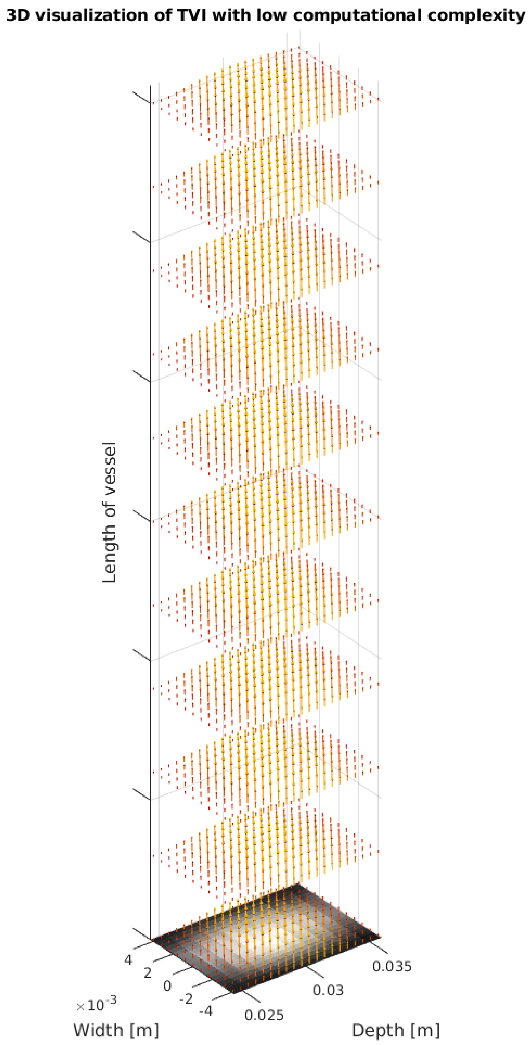
17] presented volumetric tensor velocity imaging (TVI) using a 1024 element fully addressed transducer array and computationally heavy synthetic aperture (SA) flow estimation. In TVI, the full 3D velocity vector is estimated throughout the imaged volume, providing complete flow information. An example of a tensor velocity image is shown in
Figure 1.
One major drawback of the matrix probe is that the total number of interconnections in an
element transducer scales with
. This causes issues with both fabrication and with data rates that easily exceed 100 GB/s. Morton and Lockwood [
18,
19] proposed to address the rows and the columns of the matrix array rather than the individual elements to have a linear scaling of the interconnect. Rasmussen et al. [
20] and Christiansen et al. [
21] showed how to obtain good images using such row-column (RC) addressed arrays at interconnect complexities and data rates similar to those found in current 2D systems. Holbek et al., demonstrated 3D VFI in a plane [
22] and in a volume [
23] for stationary, laminar flow, but with a very low aliasing limit of a few cm/s in the axial direction. Schou et al. [
24] demonstrated volumetric 4D (3D+time) VFI without this aliasing limit by using a computationally very expensive synthetic aperture (SA) imaging sequence, making real-time implementation extremely difficult at best. Also, Schou et al. presented volumetric flow in 4D with RC addressed array by using SA. This study was implemented for simulation and measurement and showed capability of only 62 channels in receive to make 4D volumetric imaging. To do SA the entire volume must be beamformed with every emission making real-time difficult at best. Jørgensen et al. [
25] improved SA tensor velocity estimates for RC arrays by motion compensation of low-resolution volumes. Sauvage et al., implemented Power Doppler estimation on a large 128 + 128 elements RCA with plane wave emissions [
26]. The same method was used in functional brain imaging [
27]. However, Power Doppler provides no directional information and gives only qualitative measure of blood flow, and one can not get the velocity components by this method. Moreover, in this paper were used coherently-compounded orthogonal plane waves, investigated by Flesch et al. [
28]. For that purpose is necessary to reconstruct the whole volume for every emission, which gives the similar computational complexity as SA imaging mentioned above.
This paper presents volumetric tensor velocity imaging (TVI) simulations of parabolic flow using RC addressed array and shows that TVI can be done with the same computational complexity as conventional 2D imaging and without ECG gating. Directional TO [
29] and interleaved emission sequences [
30] are combined and adapted for use with RC arrays to achieve full volumetric 3D TVI. The interleaved sequence introduced to reduce time difference between correlated signals in SA flow from
N *
to
. Achieved by interleaving two identical sequences. In this work, it is adapted to non-SA flow. The interleaved sequence is compared to a non-interleaved sequence with the same parameters.
Section 2 describes the methods including the RC array, the emission sequence, and the velocity estimator.
Section 3 presents the results, and
Section 4 and
Section 5 discusses the results and presents conclusions.
2. Methods
This section gives a brief introduction to RC arrays and explains the emission sequence and velocity estimator.
2.1. Row-Column Addressed Arrays and Velocity Estimation
The principles of a 2D RC addressed arrays are explained already in previous papers [
18,
20], and a brief introduction is given here.
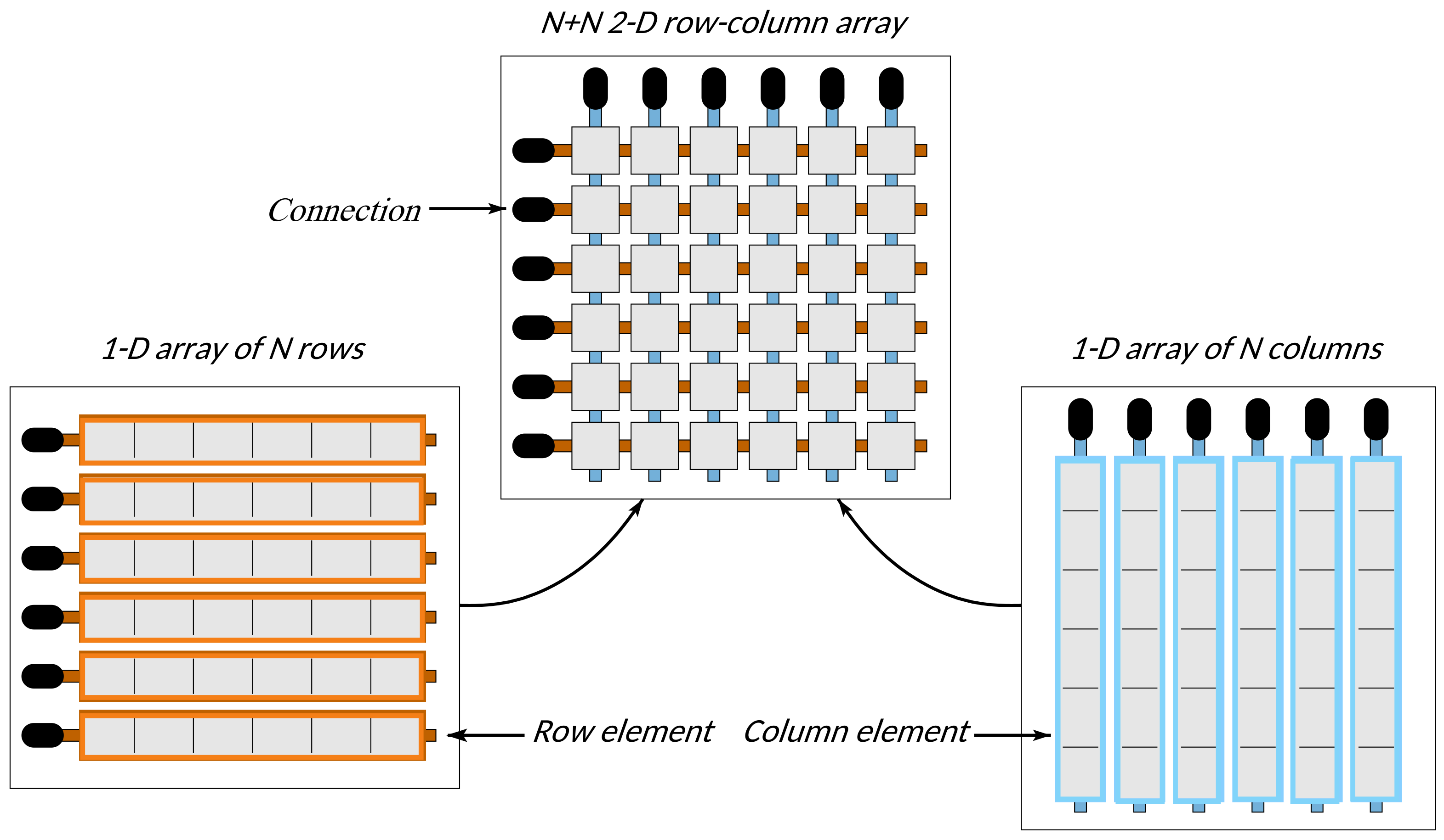
An RC addressed array can be viewed as two orthogonal 1-D arrays with tall elements, mounted on top of each other. Compared with an
matrix array, the total number of interconnections in an
RC array is reduced by a factor of
, which simplifies the interconnect and opens up for transducers with both a large footprint and a small pitch.
Figure 2 illustrates this principle.
The long elements generate cylindrical waves, and the delay-and-sum beamformer must be adjusted accordingly [
20]. Using the convention that row-elements are parallel to the
x-axis, and column-elements are parallel to the
y-axis, Holbek et al. [
22] showed that a cylindrical wave emitted by row elements allows the
x and
z velocity components to be estimated in a
-plane. Similarly, an emission with column elements allows the
y and
z velocity components to be estimated in a
-plane. The full 3D velocity vector is available in the intersection of these planes. The
x and
z velocity components are obtained in a volume by steering the beam in different directions using emissions by the rows, and the
y and
z components were measured similarly by steered column emissions [
23]. The base emission sequence employed used 9 steered column emissions followed by 11 steered row emissions that were then repeated a number of times to provide continuous data. The
nth emission in the
ith sequence was then correlated with the
nth emission in the
st sequence, i.e., the two signals given to the velocity estimator were separated in time by
, where
is the pulse repetition period. For an auto-correlation estimator, the aliasing limit
is
where
is the wavelength of the ultrasound pulse, and
is the effective pulse repetition period, which in this case was
.
This work extends on these principles and introduces modifications to overcome the aliasing limit.
2.2. Emission Sequence and Velocity Estimation
Holbek et al. [
23] steered the beam emissions by the rows and columns. A scheme of this sequence is presented below. Denoting the
mth column emission in sequence repetition
i , and the
nth row emission
, the emission sequence is written as
This sequence has the issue described above that . Such a sequence is also simulated to provide a comparison with the interleaved sequence.
Adapting the interleaved sequences for SA imaging [
30] to plane-by-plane RC TVI, the emission sequence becomes
reducing the time between two emissions being correlated to
.
The directional transverse oscillation velocity was used [
29]. To perform the velocity estimation, two sets of lines are beamformed for each emission: one set in the respective lateral direction (
x for row and
y for column emissions, respectively) and one line in the
z-direction [
29]. To estimate the velocity in a single point, the lines beamformed in the lateral direction are centered on the estimation point and span a pulse length in the
z-direction and have a two-peak apodization on the receiving aperture to induce a TO. A line length of
at
= 5 kHz corresponds to a velocity of 25 m/s. The line beamformed in the
z-direction is also centered on the estimation point, spans a pulse length and has a symmetric Hann apodization on the receiving aperture. The lateral sets of lines are pre-processed to remove the axial oscillation [
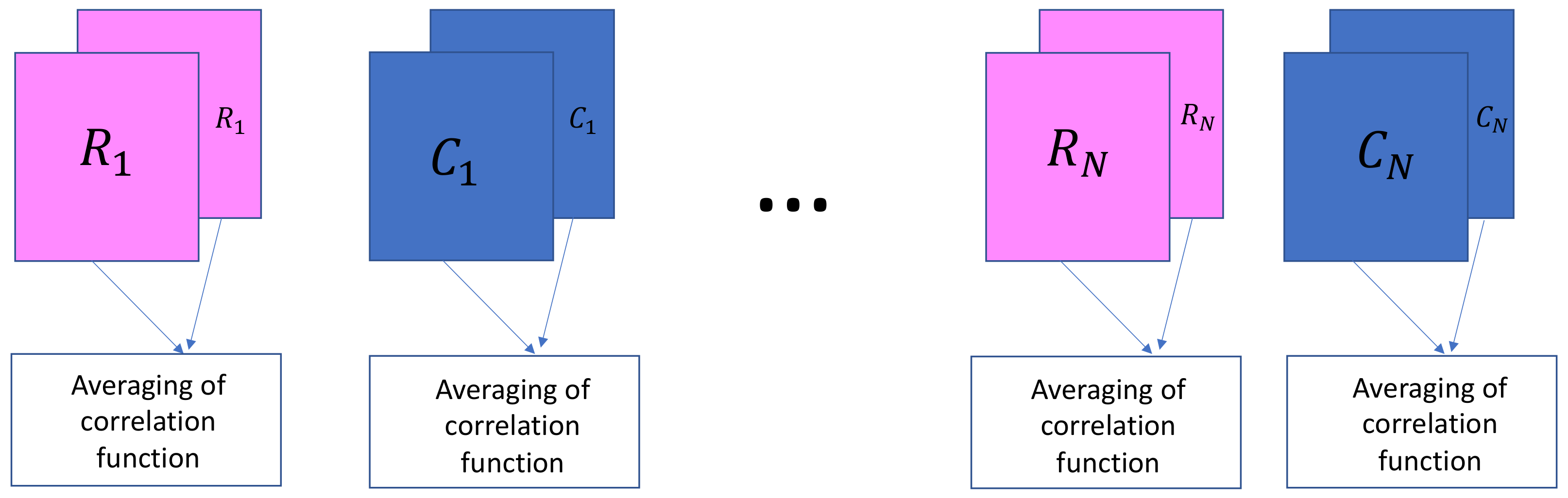
29]. The two sets of lines are correlated between emissions
and
for
i odd resulting in the correlation function
, and the
K correlation functions
are averaged. The location of the peak is found and interpolated to find the estimated velocity component. This is illustrated in
Figure 3.
In this work, , and the different row and column emissions are performed by sliding a window of 32 elements in transmit with a 9 elements step. Stationary echo cancelling was conducted by averaging 16 emissions for each direction and subtracting this mean value to remove the tissue signal.
2.3. Simulation Setup
The simulations in this study were performed using the program Field II [
31,
32]. This section describes how the simulations were carried out, and which parameters were used. The transducer, image and phantom parameters are presented in
Table 1.
A 2-D row-column array with integrated apodization was simulated with a center frequency = 3.0 MHz. The first simulation was performed for a straight vessel along the x direction.
A 4-cycles sinusoidal pulse was transmitted at from either row or column elements. The emitted ultrasound wave was focused at a line at depth of 30 mm. The pulse repetition frequency was 5.0 kHz.
A fixed symmetric Hann window spanning 32 elements was applied as apodization when transmitting the pulse from either row or column elements. In receive, a symmetric Hann window apodization across all elements orthogonal to the transmit aperture was applied for the axial velocity estimator.
A 20 × 20 × 20 mm
3 cubic phantom containing a cylindrical blood vessel (Radius = 6 mm) located at 3 cm depth was used. Scatterers inside the cylinder were translated according to a circular symmetric parabolic velocity profile, and scatterers outside the cylinder were stationary. In total, 57,600 scatterers were distributed in the phantom to ensure that more than 10 scatterers per resolution cell were present [
33]. The peak velocity
in the parabolic flow was set to 0.3 m/s.
A total of 128 frames for each vessel orientation were simulated. With a sequence length, , of 44, a total of 44 × 128 emissions were used for each parameter setup. 968 velocity profiles were estimated for the whole volume in both the lateral and transverse direction and 1936 velocity profiles in the axial directions due to the alternating between row and column emissions. 44 emissions in total were made to provide data for estimation of all components of the flow inside the vessel. Simulations were also performed for 75 and 60 degree beam-to-flow angles and 0 and 45 degree azimuth rotation. These were made with the same conditions.
2.4. Quantification of the Study
To quantify the performance when estimating the 3-D vector flow for different settings, a statistical approach was used. All estimated velocity profiles for a given setting were independent and comparable across parameter choice, as the same random number initialization seed was used for scatter distribution.
At each sample point
r inside the vessel, the mean velocity
and the standard deviation
averaged over
N frames for each velocity component, was found as
The mean relative bias
between the estimated velocity and the expected velocity
at each depth was calculated as
with
beeing the theoretical peak velocity and where
was the number of depth points. A similar relative mean standard deviation
was calculated as
The two quantitative performance metrics and were used in the study for a comparison between different parameter settings.
3. Results
In this section, the results of all simulations are presented.
First, the case with 0 degree azimuthal rotation are considered.
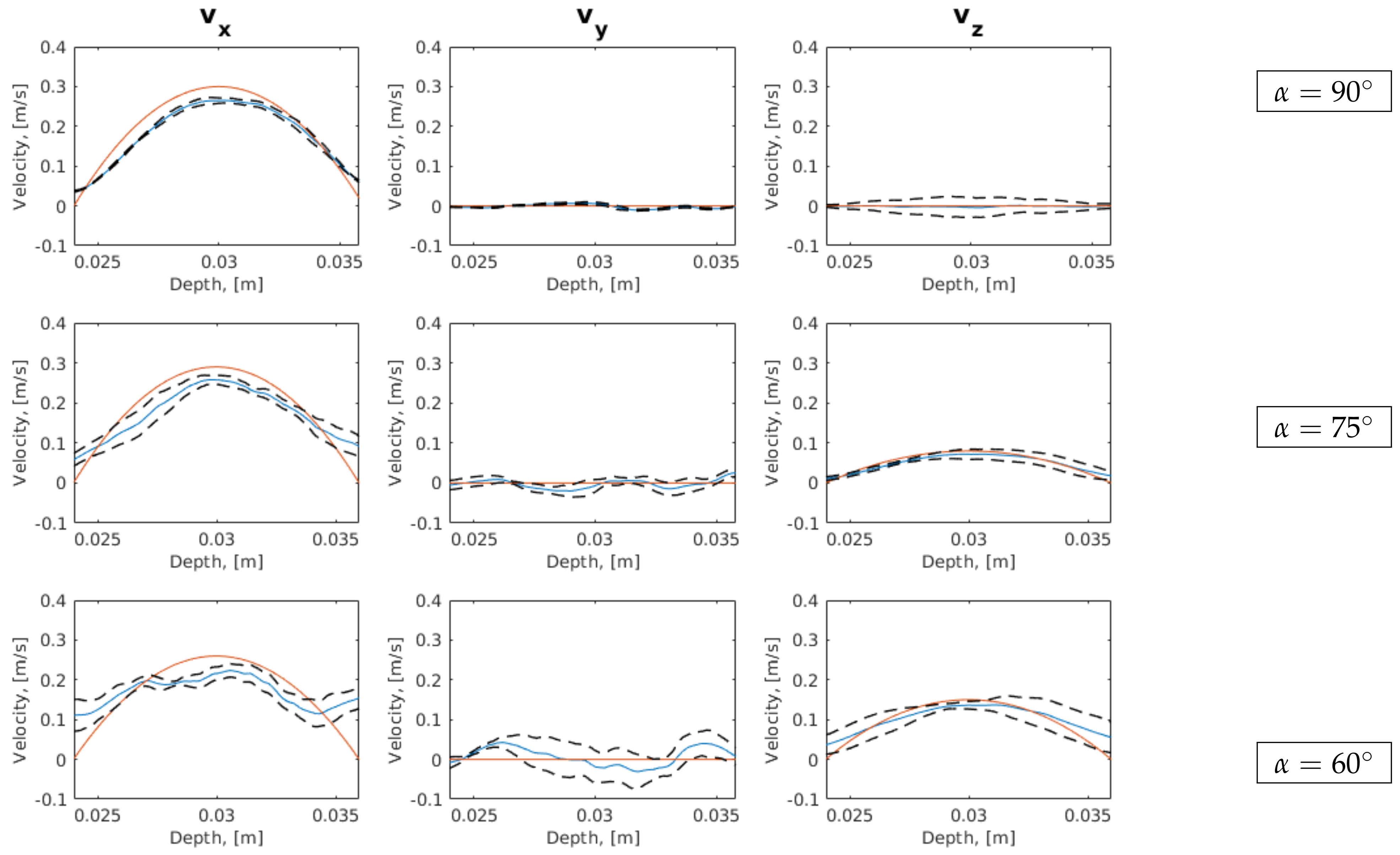
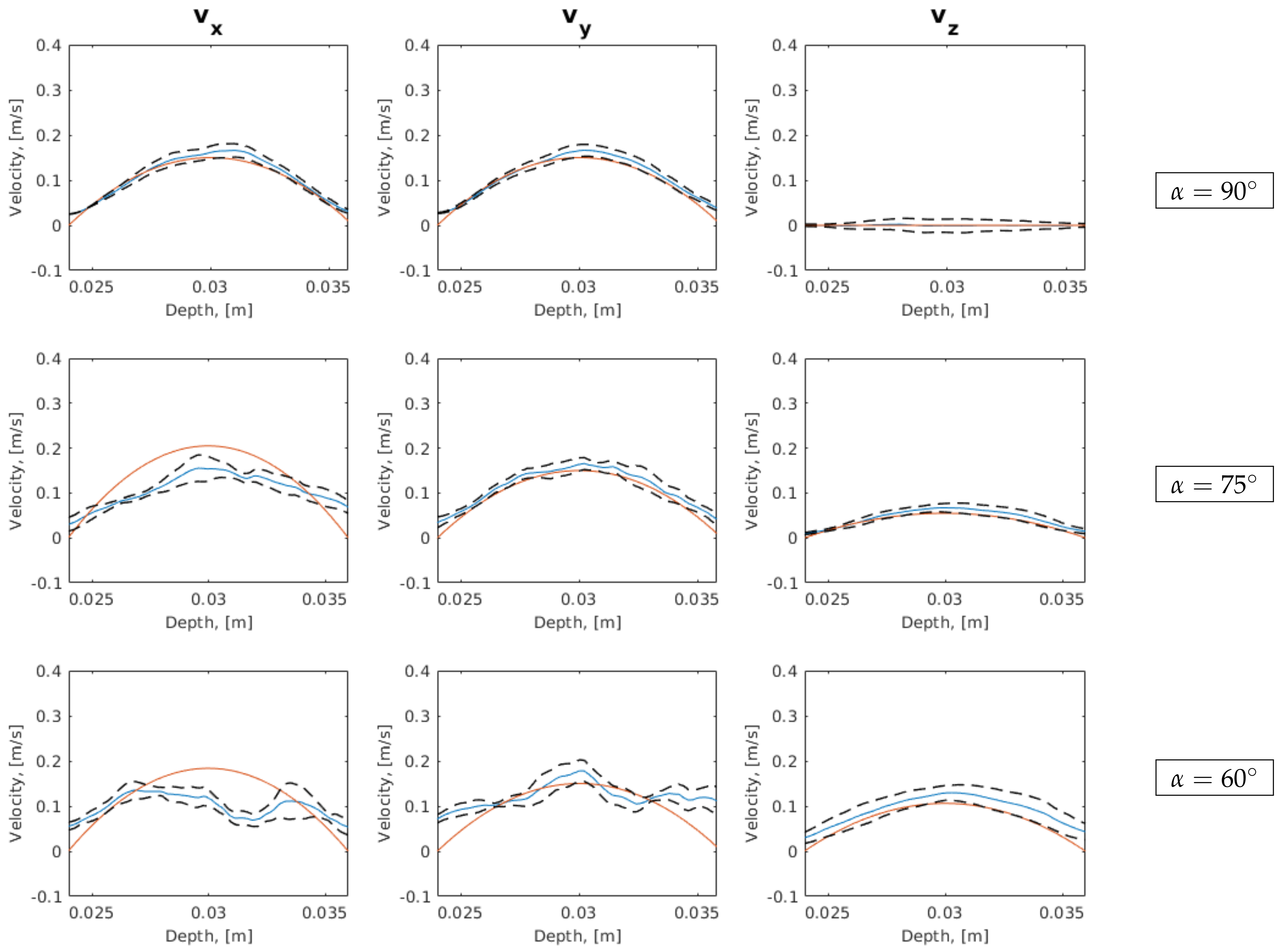
Figure 4 shows the center-line profiles along the
z-axis. The true theoretical profiles are shown in red. The blue curve is the estimated mean profile (
), and the dashed black curves shows the relative standard deviation (
).
The top row shows the case with 90 degrees beam-to-flow angle. Since the beamforming was performed along the x, y or z direction, the method is expected to perform better when the flow is parallel to one of these directions. When the flow deviates from the cardinal directions, the beamformed signals start to decorrelate, which negatively affects the method’s precision.
It is visible that the profile for the component (blue curve) of the flow matches the theoretical profile well (red line).
Further the middle and bottom rows show the cases for beam-to-flow angles of 75 and 60 degrees, respectively. These cases both have a z component of the flow as well. It can be seen that the profiles matches the theoretical profiles well. It is seen that the bias and standard deviation increase with decreasing beam-to-flow angle.
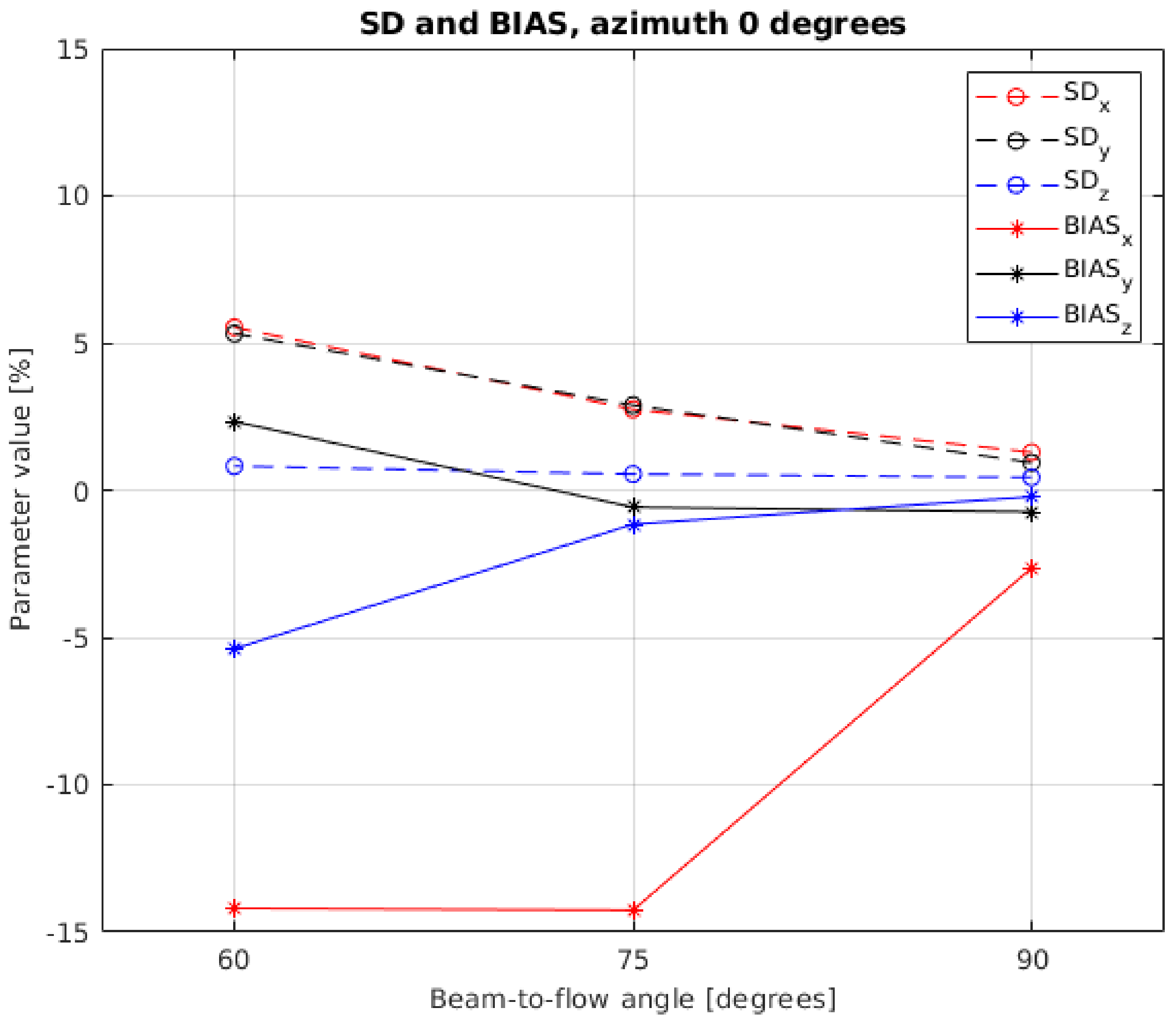
Figure 5 presents relative standard deviation (RSD) and relative bias (RB) for the entire center plane of the cases above to quantify the performance in the volume rather than along a single line. RSD is less than (1.288%, 0.934%, 0.434%) for the first case (90 degrees beam-to-flow angle) for all three velocity components (
,
,
). The RB varies from −2.64% to −0.22%. At a 75 degree beam-to-flow angle, RSD increases to 2.88% for
component. RB is also growing and varies from −0.57% to −14.25%. In the case with a 60 degrees beam-to-flow angle all parameters are increasing again. The RSD is (5.53%, 5.31%, 0.82%) for (
,
,
), respectively. The RB is (−14.1%, 2.33%, −5.38%) for (
,
,
).
Figure 6 shows the profiles along the center lines for a 45 degree azimuthal rotation and the three beam-to-flow angles.
The top row presents the case with a 90 degrees beam-to-flow angle, the middle row for 75 degrees, and the bottom row presents for 60 degrees. For all these cases the flow will also have a y-component. Good correspondence is seen between estimated and true profiles, although with increasing deviations when the beam-to-flow angle is decreased.
Comparing
Figure 4 and
Figure 6, it is seen that changes to the beam-to-flow angle have greater effect than azimuthal rotation. This is supported by the RSD and RB in
Figure 5 and
Figure 7.
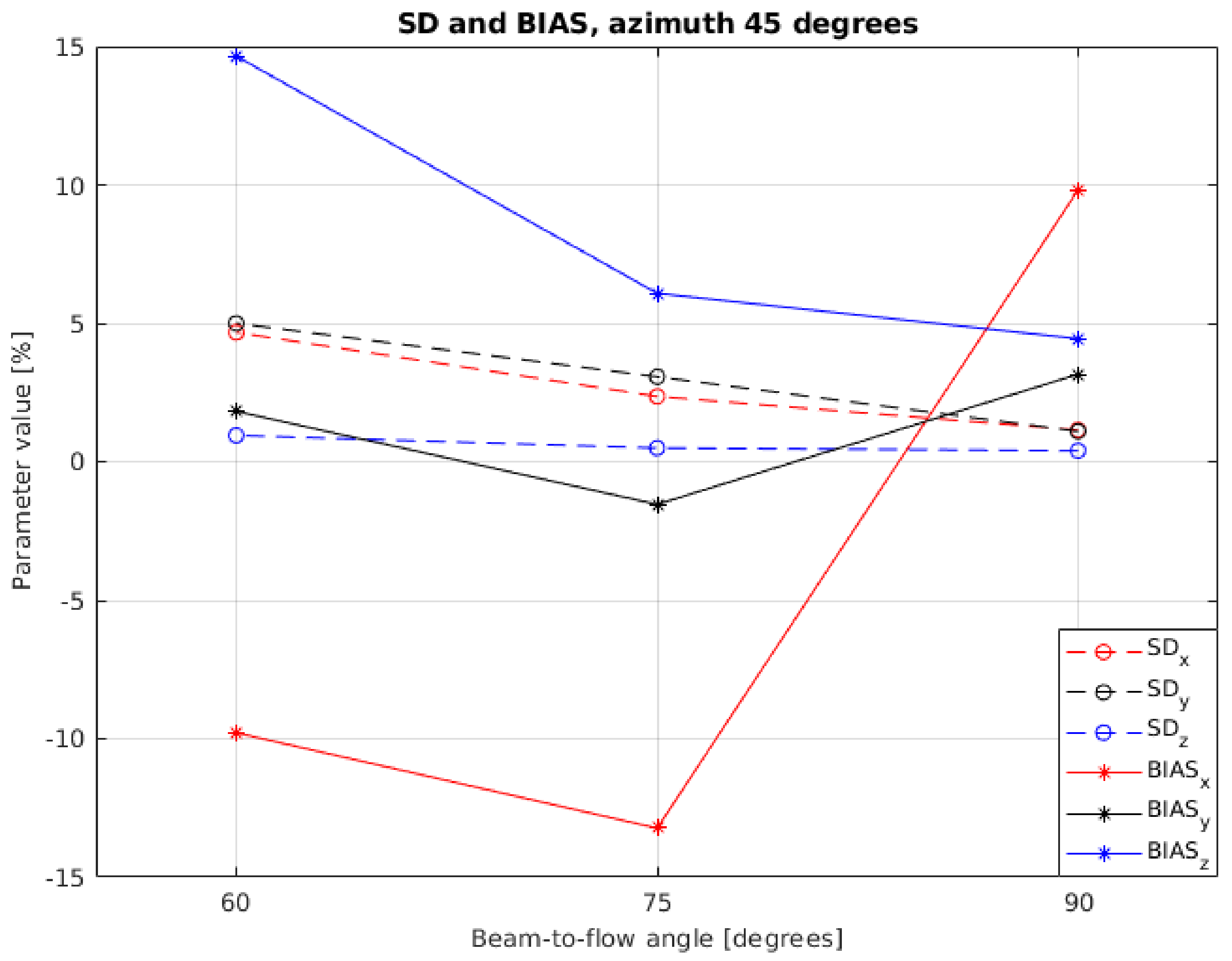
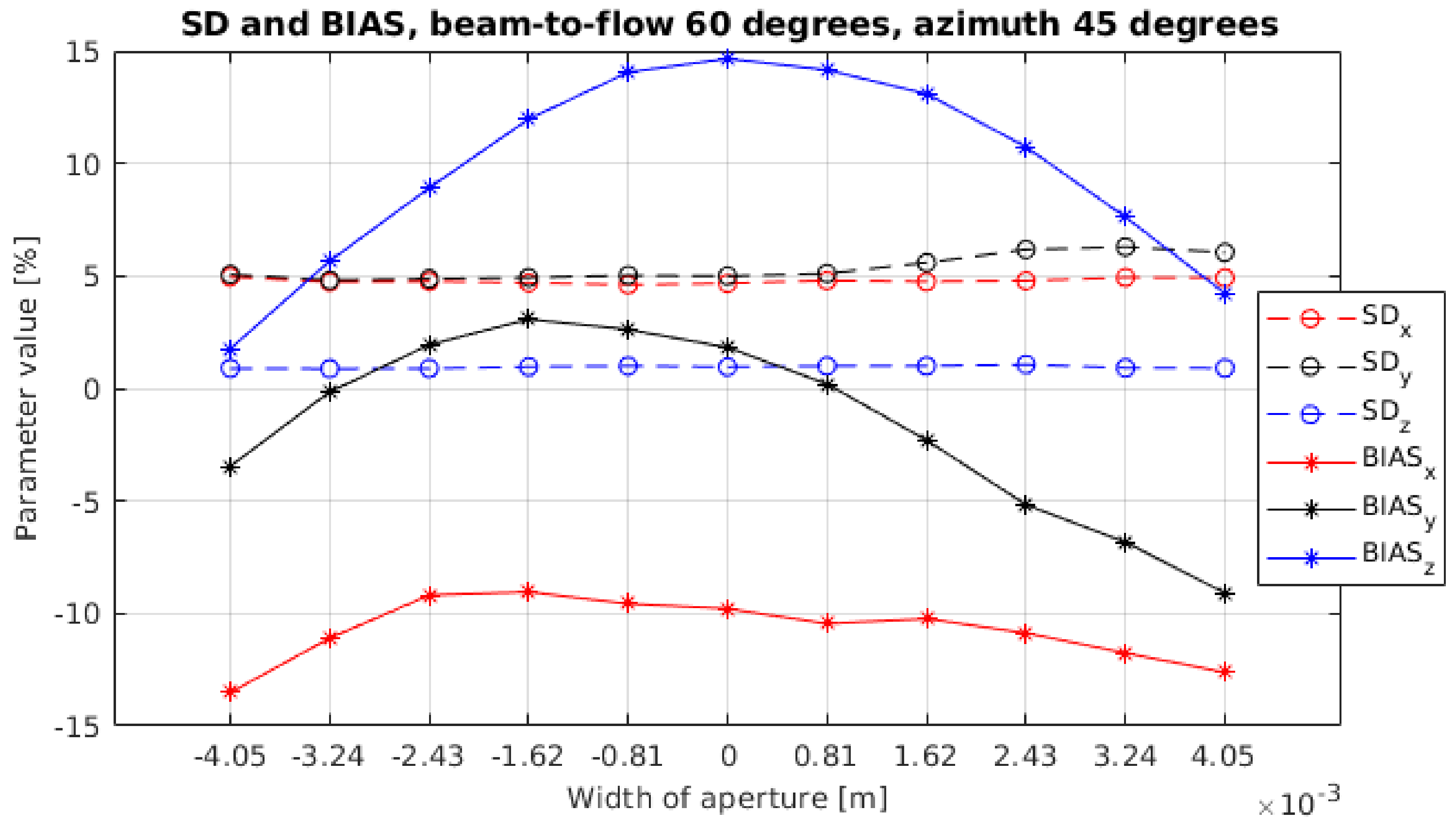
Figure 7 shows the RSD and RB for three cases from
Figure 6, again calculated from the entire center plane. One can see that the RSD is (1.15%, 1.10%, 0.39%) for 90 degrees beam-to-flow angle, the RB is (9.81%, 3.16%, 4.45%). The RSD for 75 degrees beam-to-flow angle (2.36%, 3.07%, 0.49%) and the RB is (−13.23%, −1.54%, 6.08%). The RSD for 60 degrees beam-to-flow angle is (4.67%, 4.99%, 0.96%) and the RB is (−9.78%, 1.82%, 14.65%). It is visible that the RSD is the same for cases without a rotation angle and for cases with 45 degrees rotation angle as stated above, but the RB shows larger variations.
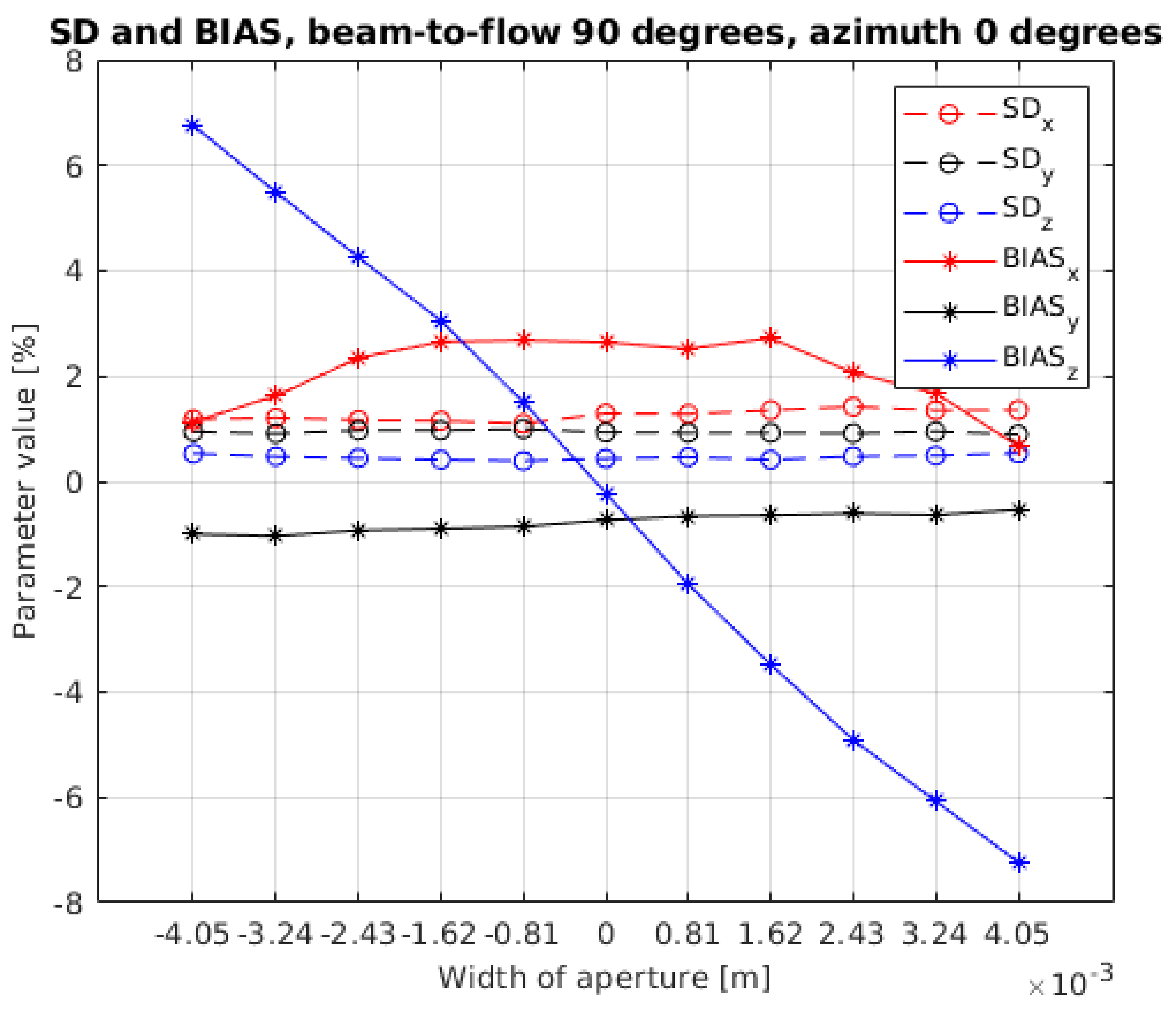
Figure 8 presents statistics for the case with a 90 degrees beam-to-flow angle and 0 degrees rotation angle for all 11 planes along the vessel. The RSD varies between 1.09% and 1.41% for
, between 0.89% and 0.99% for
, between 0.39% and 0.54% for
components of the flow. The RB for
varies between 0.67% and 2.72%, between −1.04% and −0.53% for
and for
component is between −7.23% and 6.75%. The
component was estimated using the full Hann apodized aperture. This effectively introduces an angle between the axis of the array and the line used to estimate the
component, which causes a bias in the estimates.
Figure 9 shows the RSD and the RB for 60 degrees beam-to-flow angle and 45 degrees rotation angle for all 11 cross planes along the vessel. The RSD varies between 4.61% and 4.95% for
, between 4.81% and 6.29% for
, between 0.88% and 1.06% for
components of the flow. The RB for
varies between −13.52% and −9.04%, between −9.09% and 3.08% for
and for
component is between 1.76% and 14.65%.
On both
Figure 8 and
Figure 9 the RB varies for the
component with position in the imaged volume.
4. Discussion
Plane-by-plane interleaved technique for TVI in a full 3D volume using TO in combination with a cross-correlation estimator was investigated. Implementation and validation was performed by simulations. In this paper TO was combined with a sliding aperture sequence. The highest RSD is 6.29% and is calculated for the case in which the beam-to-flow angle is 60 degrees and 45 degrees of rotation angle. The lowest RSD is 1.288% for non-zero component and is calculated for 90 degrees beam-to-flow angle and 0 degrees rotation angle.
For comparison, a non-interleaved sequence was also simulated with the same setup in all other aspects. Such method was first presented by Holbek et al. [
22] who achieved 8.7% of RSD for 90 degree beam-to-flow angle. They used
= 10 kHz and 9 + 11 steered planes. Here, the non-interleaved sequence was simulated for
= 5 kHz and for
= 10 kHz.
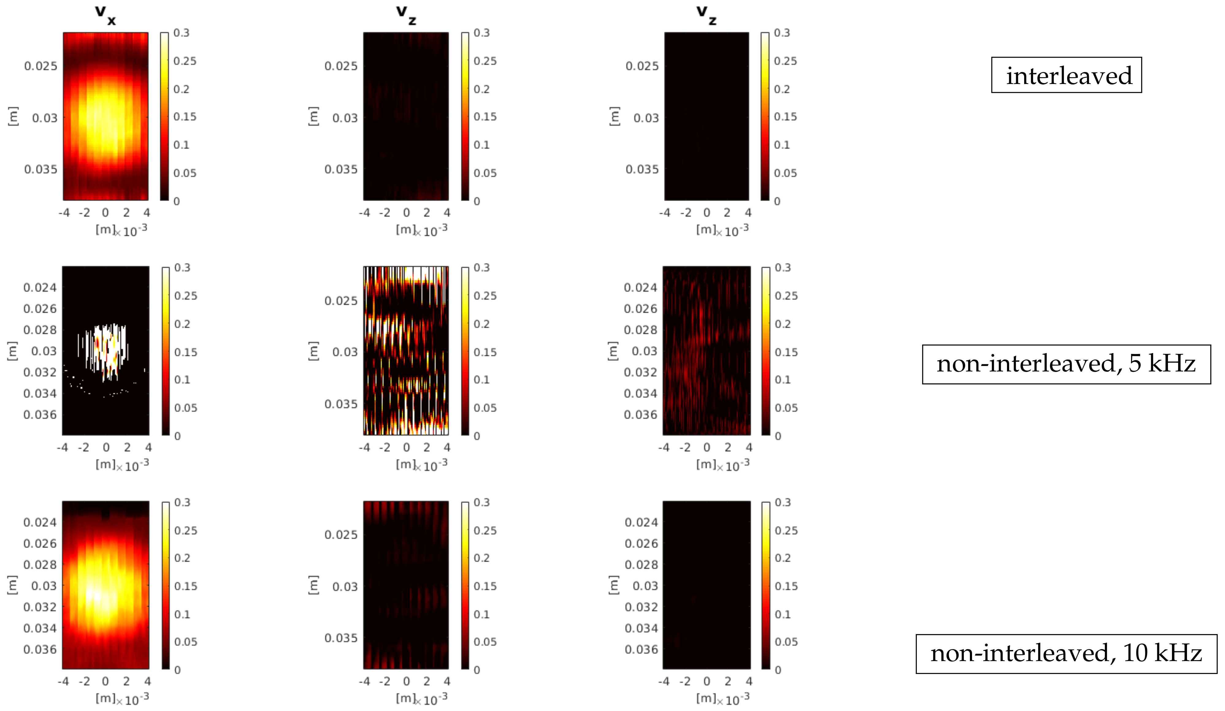
Figure 10 presents results for 90 degrees beam-to-flow angle and 0 degrees rotation angle for interleaved, non-interleaved with
= 5 kHz and non-interleaved with
= 10 kHz.
Cross planes for each velocity component are shown for all three sequences, which were mentioned above. The top line shows cross planes for the interleaved sequence with
= 5 kHz, and the second line shows the non-interleaved sequence with
= 5 kHz. On the bottom line the non-interleaved sequence with
= 10 kHz is shown. As seen, the non-interleaved sequence with
= 5 kHz (middle line) fails to estimate the flow. In comparison, the interleaved sequence and non-interleaved with
= 10 kHz show good results. The time between lines being correlated is
for the interleaved sequence and 22
for the non-interleaved sequence. At
= 0.3 m/s, the scatterers move 0.06 mm or
between the emissions correlated for interleaved sequence, 1.32 mm or
for non-interleaved sequence with
= 5 kHz and 0.66 mm or
for non-interleaved sequence with
= 10 kHz. Holbek et al designed their sequence in this way to have continuous data throughout the volume [
22]. The interleaved sequence attains this goal with only 1 Tprf between correlations.
Full 3D velocity vector field in a volume by row-column addressed array was presented by Schou el al. [
24]. They also used an interleaved sequence and SA imaging, which requires beamforming of the entire volume for all emissions. Our method only needs beamforming of small sub-planes for
and
components of the flow and only one line for the
component. Thus, in the method presented here, the
velocity component requires 188 samples to beamform, and the
or
components requires 1474 samples each. The SA method requires 11 times as many beamforming operations per emission. In
Table 2 the results of Schou et al and the method in this work are compared. The top part shows the RSD and RB for 90 degrees beam-to-flow angle and 45 degrees rotation angle. The bottom part shows the RSD and RB for 60 degrees beam-to-flow angle and 45 degrees rotation angle. Our method attains a smaller RSD, but a higher RB. However, the small RSD enables compensating for the RB.
Jørgensen et al. [
25] expanded Schou’s work [
24] to add motion correction to improve the velocity estimation. However, due the motion correction the SA beamforming needs to be done multiple times for each estimate. It improved on the method without motion compensation, but at the expense of at least twice higher computational complexity than SA flow without motion compensation.
TVI has been investigated in other works as well. Makouei et al. [
34] did TVI using a fully addressed, 1024 element matrix array and synthetic aperture imaging. A RSD of 1.46% was attained for the same range of vessel orientations, but at a more shallow depth. This study also used SA imaging with beamforming of the full volume for all emissions. It used a 1024-element fully addressed array, which require 8 times more channels for 1/4 surface area of the array at the same center frequency compared to RC addressed array. Scaling the fully addressed array to the same size as the 62 + 62 RC array used in this work, the computational complexity is increased 62 times in addition to the increase in complexity from SA imaging. Such a method would furthermore require a system with 4 k channels, which is 16 times more than modern commercial systems have.
Wigen et al. [
16] presented 4D vector flow imaging using a commercial 2D matrix array transducer with ECG-gating. The ECG-gating is utilized to separate a full volume into multiple sub-volume acquisitions. They also used a subaperture beamforming (SAP) to perform a partial in-probe beamforming to reduce the number of channels coming from the transducer with a subsequent beamforming stage in the system. After that to make second beamforming stage is necessary. The computational complexity of this method is comparable with SA imaging. RSD and RB were presented in absolute units (m/s) and from a different evaluation setup with a spinning disk. By normalizing with the peak velocity of this disk as done in (
7), gives a RSD of 1 to 3%, which is comparable to the results of the method presented here.
Commercial ultrasound systems handle 128–256 transducer channels, and they can beamform around 16–32 lines in parallel. These values are comparable to the method, presented here. The computational complexity thus is similar to what is performed in modern ultrasound systems, and this method should be implementable on such systems. In comparison, SA imaging or other methods with similar computational complexity can currently not be implemented in real-time on such systems.
In the review paper by Jensen et al. [
35] results for different techniques were presented. For 2D vector flow imaging (VFI) RSD is typically between 5.5% and 14.7%. As was shown in this work, TVI with low computational complexity can provide similar precision. Additionally, VFI and TVI are angle-independent methods that do not require the beam-to-flow angle to be estimated by hand as it does in e.g., spectral Doppler, which is commonly used in the clinic. 2D VFI has been shown to measure peak systolic velocities (PSV) that agree with magnetic resonance angiography, as opposed to spectral Doppler that overestimates the PSV [
36]. 2D VFI only measure two of the three velocity components, thus TVI can be expected to perform comparably or better.


