
A Machine Learning Method Based on 3D Local Surface Representation for Recognizing the Inscriptions on Ancient Stele


1
Future Convergence Engineering, Department of Electrical, Electronics and Communication Engineering, Korea University of Technology and Education, Cheonan 31253, Korea
2
Future Convergence Engineering, Interdisciplinary Program in Creative Engineering, Korea University of Technology and Education, Cheonan 31253, Korea
*
Author to whom correspondence should be addressed.
Appl. Sci. 2021, 11(12), 5758; https://0-doi-org.brum.beds.ac.uk/10.3390/app11125758
Submission received: 6 May 2021
/
Revised: 10 June 2021
/
Accepted: 12 June 2021
/
Published: 21 June 2021
Abstract
:It is challenging to extract reliefs from ancient steles due to their rough surfaces, which contain relief-like noise such as dents and scratches. In this paper, we propose a method to segment relief region from 3D scanned ancient stele by exploiting local surface characteristics. For each surface point, four points that are apart from the reference point along the direction of the principal curvatures of the point are identified. The spin images of the reference point and the four relative points are concatenated to provide additional local surface information of the reference point. A random forest model is trained with the local surface features and, thereafter, used to classify 3D surface point as relief or non-relief. To effectively distinguish relief from the degraded surface region containing relief-like noise, the model is trained using three-class labels consisting of relief, background, and degraded surface region. The initial three-class result obtained from the model is refined using the k-nearest neighbors algorithm, and, finally, the degraded region is re-labeled to background region. Experimental results show that the proposed method performed better than the state-of-the-art, SVM-based method with a margin of 0.68%, 3.53%, 2.25%, and 2.36%, in accuracy, precision, F1 score, and SIRI, respectively. When compared with the height- and curvature-based methods, the proposed method outperforms these existing methods with accuracy, precision, F1 score, and SIRI gains of over 4%, 20%, 11%, and 12%, respectively.
1. Introduction
Stone monuments are important artifacts that provide artistic, cultural, political, or historical background to events during the time they were created [1]. Due to the long exposure of these stones to wind, heat, rain, animal activities, and other factors in the environment where they are located, their surfaces degrade over time [2,3]. As a result, the contents (or information) which are sometimes in the form of ancient characters or drawings carved on the surfaces fade before archaeologists excavate them. One of the problems that archaeologists encounter after collecting these stones is how to accurately recover the information on the external surface of the monuments.
In the past, the stone rubbing method was commonly used to recover inscriptions on monuments. This method extracts important features from the surface of the stone by rubbing rendering materials over paper placed on top of the stone monuments [4]. The quality of the relief extracted through this method depends on the professional experience of the epigrapher. If the technique is applied carelessly, the cultural monuments which have undergone abrasion can be further damaged or contaminated. To prevent damages and avoid labor costs for repairs, non-physical methods for extracting relief from monuments have received considerable attention lately in the field of computer graphics and computer vision [5,6,7,8,9,10]. The decorrelation stretch (DStretch), an image processing plug-in made by Defrasne [5], was applied to enhance images of faint reliefs carved on rocks [11]. DStretch involves the application of the Karhunen–Loeve transformation to a 2D colored image of the surface of a rock to obtain a 3 × 3 transformation matrix. The product of the obtained transformation matrix and the image that contains faint reliefs on rock produced a new image with enhanced reliefs. However, the performance of this functional software is not reliable in extracting reliefs when the surfaces of the monuments contain severely damaged regions. In another study, a feature extraction method, known as the Hough transform, was used for the representation of surface features by applying the feature curve approximation function to a family of curves [9]. This transformation was demonstrated to be effective in the recognition of decorative patterns from the surface of defective or severely degraded archaeological objects. Recently, Romanengo et al. [10] extended the application of Hough transform for surface representation by defining new set of rules and conditions for selecting suitable curve approximation that guarantees reliable recognition of decorative surface points. Furthermore, new curve models were analyzed and added to the existing family of curves to increase the accuracy of identifying the characteristic curves.
With the introduction of sophisticated 3D scanners, it is now realistic to extract reliefs from 3D scanned surfaces of stone monuments. The 3D scanned monument is represented as surface mesh with triangular faces. Several 3D data processing techniques can thereafter be applied to the 3D mesh to gain meaningful insights about the ancient monuments, such as changing the angle of views at various scales without optical illusions in the material pattern or discoloration [6,7,12,13,14,15]. Scanning defects in the form of outliers, noise, ghost geometry, and holes are usually introduced to the 3D mesh surface during the scanning process. A set of tools based on point modeling techniques was presented to address these problems [16]. The point modeling techniques mainly involve data structures, i.e., the moving least square optimization and point relaxation functions. Another post-processing method based on normalized vector field was introduced and applied in operations such as surface smoothing, details enhancement, and artificial coloring of the 3D scanned surface [6].
Considering a smooth base normal, a relief extraction technique that estimates the height distribution of reliefs and background by integrating relative heights between adjacent vertices was presented by Zatzarinni et al. [8]. The normals of the base surface were first estimated to determine the height of the surface points and a Gaussian mixture model was applied to the height distribution to obtain a threshold that was used to decide if a surface point is a relief or background. Degraded regions were identified and removed using a filter that relies on the size and shape of the identified regions. This technique was demonstrated to be reliable in applications such as detail exaggeration and dampening, cut and paste of relief, and drawing of prominent curves. Recently, a digital 3D stone rubbing approach which also estimates the heights of mesh vertices using a weighted least square method was presented by Pan et al. [15]. The estimated heights were transformed subsequently to grey values using a nonlinear transformation function. The transformed heights were segmented into black, white, or grey colors based on the relationship between the individual height and the mean and standard deviation of the heights of neighboring vertices. In this manner, a digital stone rubbing similar to the traditional rubbing was determined from the 3D mesh.
Following the successful application of the Frangi filter in the detection of blood vesselness [17], a modified Frangi filter was developed to extract relief details from the surface of 3D mesh [7,18]. Considering the canal-like shape of the reliefs, curvatures are intuitive and effective measures for detecting reliefs. At a position corresponding to the relief, its minimum and maximum curvatures, and , would be close to zero and a large value, respectively. The earlier modification of the Frangi filter is based on the computation of curvature to obtain carvings. This is achieved by clustering the surface regions and using a measure of saliency to rank the detected carvings on weathered plasters [7]. In addition, the authors presented a flexible and interactive tool with simple visualization for modifying reliefs. While this method is not suitable for extracting reliefs from the rough surfaces of stele because the presence of degraded regions disrupt the ranking of the saliency, another variants of the Frangi filter handles this problem by applying two vesselness values of different curvature sizes and selecting an acceptable threshold to effectively remove the irregular surface regions [18].
A handful of machine learning techniques have been introduced lately to analyze prehistoric cultural heritage [19,20,21]. The features extracted from these monuments can include the textural information of the soil samples of the monuments or the digital contents of the 2D/3D images that are captured by electronic cameras and scanners. Liu et al. [22] presented a supervised machine learning method to refine bas-relief surfaces for reversed engineering. Initially, the surface of the bas-relief was segmented using a snake-based method and the background region was estimated using b-spline surface fitting curves. Although the results obtained are promising, the roughness nature of the surface of the stele affects the performance of this method. In addition, the method considered only the relief and background labels, and ignored the degraded surface region. The use of the two-class labels affects the performance of these models since the degraded surface region share geometrical features similar to the reliefs, and this interferes in the conditions set for extracting reliefs [23].
More recently, support vector machine (SVM) was applied to extract relief region from the surface of stone monument [24]. The modified curvature-based method [18] was initially used to identify relief candidate segments from mesh partitions. The relief candidates include actual reliefs and relief-like noise. From each candidate segment, 79-dimensional geometrical features were extracted, which consist of the appearance, quadratic approximation for cross section, and local extrema of the candidate segments. The geometrical information was learned by the SVM to determine whether the candidate is relief or not. While this machine learning method outperformed the height estimation [8] and curvature-based methods [7,18], the superior performance of the SVM-based method [24] is largely dependent on the local surface features that were identified on the 3D mesh and the conditions for the removal of degraded region.
In this paper, we consider the spin image (SI) as features to describe the local surface of 3D mesh. SI is widely used in computer vision and computer-aided design because of its efficient shape representation of 3D objects which was posed as surface matching problem [25]. The effectiveness of SI for describing the surface of steles had been promisingly demonstrated [26]. The main contribution of this paper is the training of a machine learning classifier based on the SI descriptions that are extracted from the 3D mesh of very rough stele. In order to effectively distinguish the relief region from the background surface, we enhance the representation of the SI description by structurally configuring multiple SIs. Considering the canal-like shape of the reliefs, the minimal curvature direction, follows the canal at a position within the relief, while the maximal curvature direction, climbs up the canal along the cross section. As a result, the locations apart with a certain distance along from the given relief position tend to belong to the identical relief, while the locations apart along would be the background. Using the principal curvature directions at a particular vertex with reference, four relative surface points are identified on the 3D mesh. We refer to the aggregation of the SIs of these five points including the reference and its four relative points as cross spin image (CSI). In the proposed approach, the CSIs are extracted as features per vertex to train a three-class label random forest (RF) model. The class labels of the surface points include the relief, background, and the degraded region. The k-nearest neighbors (k-NN) algorithm is used to refine the classification results. The degraded region is identified and re-labeled to background region. As such, the proposed method classifies the surface points as relief or non-relief region. In contrast with the SVM-based method which classifies relief using candidate segment [24], the classification of the proposed machine learning-based method is done per vertex.
The remaining sections of the paper are divided as follows: Studies relevant to the proposed method are discussed in Section 2. We present the proposed approach in Section 3. Various parameters used in the proposed method are determined and the performance of the proposed method is compared with existing techniques based on intuitive geometrical features in Section 4. Finally, we conclude our findings in Section 5.
2. Related Work
2.1. Basic Geometrical Features
In this subsection, we discuss the two conventional geometrical feature-based relief extraction methods: height (depth)-based and curvature-based methods. The height-based method is one of the simplest and most prominent methods for relief extraction [8]. The height estimation of the new surface point is considered using a given path on the mesh surface with the surface normal vector. The height estimate at on the surface along the path from to is given as
where is the reference point location on the surface mesh, and the vertices along the path are , such that , and is the base normals associated with each corresponding edge between two vertices. Assuming that the heights of the reliefs and background follow Gaussian distributions, respectively, the Gaussian mixture model is applied to determine the threshold that intersects the two height distributions. This implies that the accuracy of this technique relies on the selection of a good threshold value. Furthermore, depth cannot be an absolute measure for detecting reliefs because dents and cracks on the surface of the stele can also be deep, particularly in a severely weathered stele.
For the curvature-based methods, the authors exploited the distribution of surface curvatures to extract reliefs from wall carvings [7,18]. Letting and () denote the minimal and maximal curvatures, respectively. In a relief region, it is expected that and . The Frangi filter is modified and applied to measure the vesselness, , at each vertex within the surface mesh as [17]
where A and B are and , respectively, and and are parameters that are used to control the effect of the first and second term of the filter. From Equation (2), when , the first term identifies regions of interest relating to the local shape of the surface. This term becomes large when the local surface is curved like a valley. The second term is related to the structure of the local surface and increases as the valley becomes steep and deep.
After the vesselness, , for all the vertices has been determined, vertices with non-zero values of are identified as reliefs and the zero values as background. However, the computation of the curvatures requires derivative operation, and thus is prone to be affected by noise from the scanning process and the roughness of the surfaces of the monuments. These noisy curvatures give inaccurate vesselness values because of the small marginal difference in the principal curvatures, which result in unsatisfactory reliefs.
2.2. Relief Extraction Using Machine Learning
Among the machine learning models with acceptable performance in the extraction of reliefs is the SVM-based approach [24]. The main idea of this method involves the initial extraction of relief candidate segments which includes actual reliefs and relief-like noise (cracks/dents). Then, various geometrical features are extracted from the candidate segments, and, lastly, the SVM model is trained to carefully determine if each candidate is actual relief or non-relief. The relief candidate segments are extracted from the stele using the modified curvature-based method [18]. The geometrical features extracted from the segments consist of appearance, cross-section, and local extrema information.
The size and positions of relief candidate segment are important parameters for describing the appearance of objects. While the number of vertices in the segment determines the area of the segments, the statistical values of the surface points and their corresponding normalized surface points of the relief segments provide useful information relating to the positions of the surface points that are identified within the candidate segments. To obtain the cross-section features, 2D skeleton information of the segments are derived from the x- and y-coordinates of the surface points within the segments. The width and depth of the cross section and the magnitude of the curvatures are extracted as the cross-section features. For the local extrema information, the location of the maximum depth point along the skeleton of the segments is considered. This local feature relies on the depth value and the distance separation between the point of interest and the skeleton.
The numbers of features extracted for the appearance, cross-section, and local extrema are 31, 25, and 23, respectively. Altogether, these features are used to train a binary SVM classifier with a third-order polynomial kernel.
2.3. Spin Images
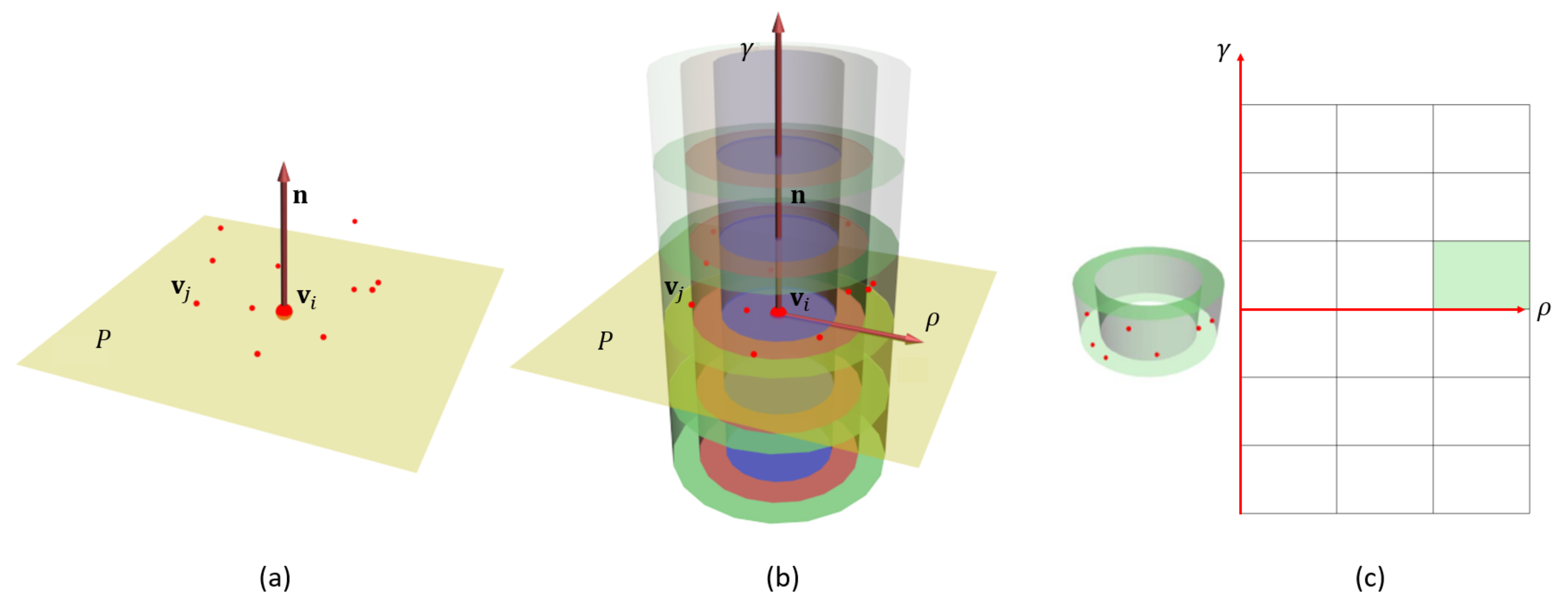
Many papers describe the characteristics of local surfaces of 3D objects [27,28,29,30,31,32]. Spin image representation, one of the local surface descriptors, has been widely used for face recognition and object classification. Originally, the technique was introduced to address the problems of surface matching in computer vision [25]. The generation of SIs on the surface of a 3D object can reveal the local structural properties around each surface point. Assume that oriented points are distributed in the 3D space, each point is represented as a pair of its position and normal vector , as shown in Figure 1a.
An imaginary plane P that contains and has the same normal divides the 3D space around into two non-overlapping subspaces: the upper subspace above the plane and the lower subspace below it. Similarly, several imaginary planes that are parallel to P and equally spaced apart from each other also divide the space into smaller non-overlapping subspaces. Each subspace can be further partitioned radially from based on the distance to , as shown in Figure 1b. The SI for a certain oriented point (, ), denoted by , is computed by encoding the coordinates of neighboring points, , around into a 2D histogram with two indices, and , as shown in Figure 1c. Specifically, the coordinates of the SI, and , indicate the indices of discrete intervals defined along the radial direction from and the direction of , respectively. As a result, a bin of the SI represents a cylindrical space with a hole whose axis coincides with , as shown in the left image in Figure 1c, and the bin value indicates the number of points belonging to the space. The mathematical representation of the spin image coordinate of any 3D surface point, , is mathematically given as
The generation of SI is dependent on the bin sizes and image dimension. While the bin sizes and determine the volume of each cylindrical subspace, the image dimension is the number of rows, , and columns, , of the SI.
3. Proposed Method
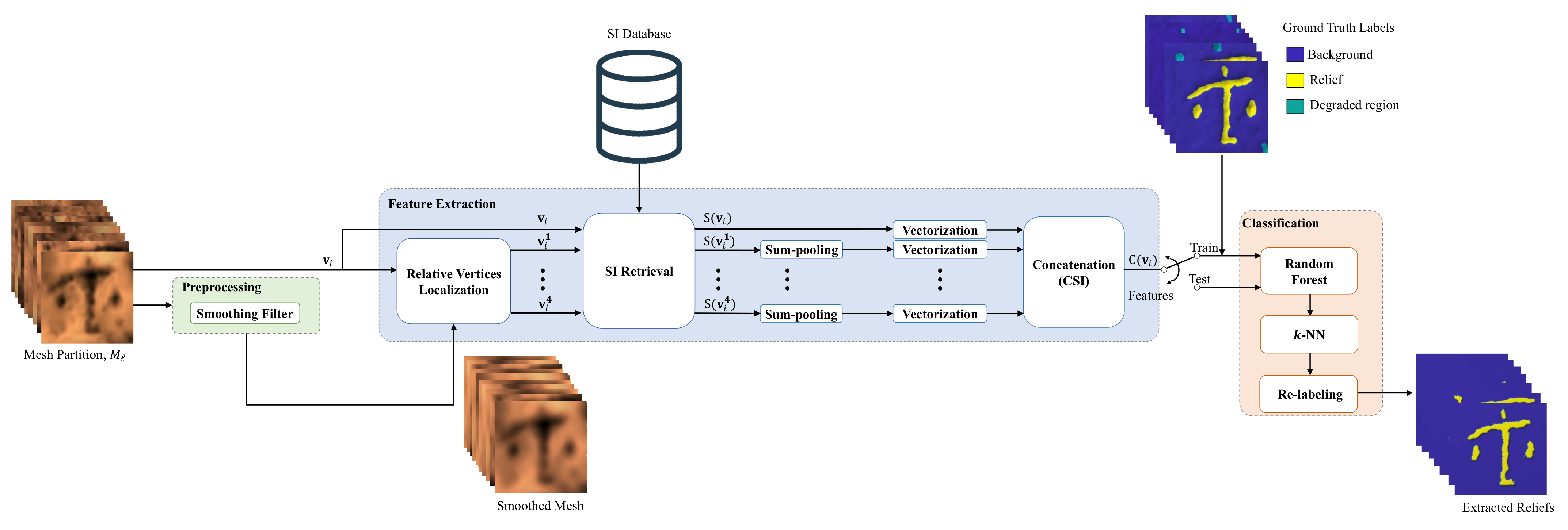
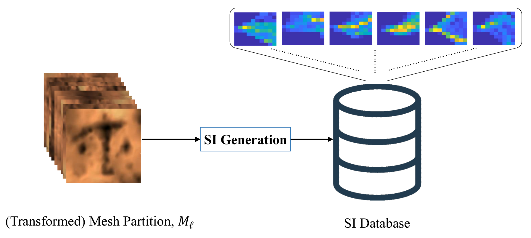
We present the proposed approach of extracting relief regions from the stone monuments in this section. A simple block diagram of the proposed relief extraction method is shown in Figure 2. Mesh partitions that contain identifiable characters are cropped from the 3D mesh. For very uneven steles, the cropped mesh partition can be slanted. To correct this, principal components of vertices of the mesh partition are obtained using the principal component analysis. The mesh partition is transformed to make the eigenvector corresponding to the smallest eigenvalue point vertically upward. The transformed mesh partition is denoted by . The generation of SI involves the creation of SI for every vertex of all the 3D mesh partitions, and the information is stored offline in an SI database (Figure 3). For a reference vertex , four relative surface points, , , , and , are searched along the bi-directions of the two principal curvatures. The five SI representation, , , , , and , are easily queried offline from the SI database.
The simple concatenation of the five SIs, however, causes the feature dimension to increase five times. In order to avoid overfitting and training time increase, the dimensions of the SIs of the four localized vertices are reduced effectively by the sum-pooling operation. The spin image information of the five vertices are merged to form a feature vector, which is referred to as the CSI of and is denoted by . The CSI is used for the training of a three-class label RF model.
Classification per vertex may cause isolated misclassified vertices. The k-NN algorithm is applied to correct such noisy misclassification, which improves the performance of the proposed method as well as enhances the visualization of the classification results.
3.1. Preprocessing
As mentioned above, the roughness nature of the surface of the ancient stele hinders the reliable estimation of surface curvatures. To address this problem, the input mesh is smoothed using the Gaussian filter with the standard deviation before estimating the curvatures. It is notable that the smoothed mesh is exploited only for curvature calculation. The SIs are generated using the original mesh without smoothing.
3.2. CSI Feature Extraction
The modules involved in the feature extraction process are explained as follows:
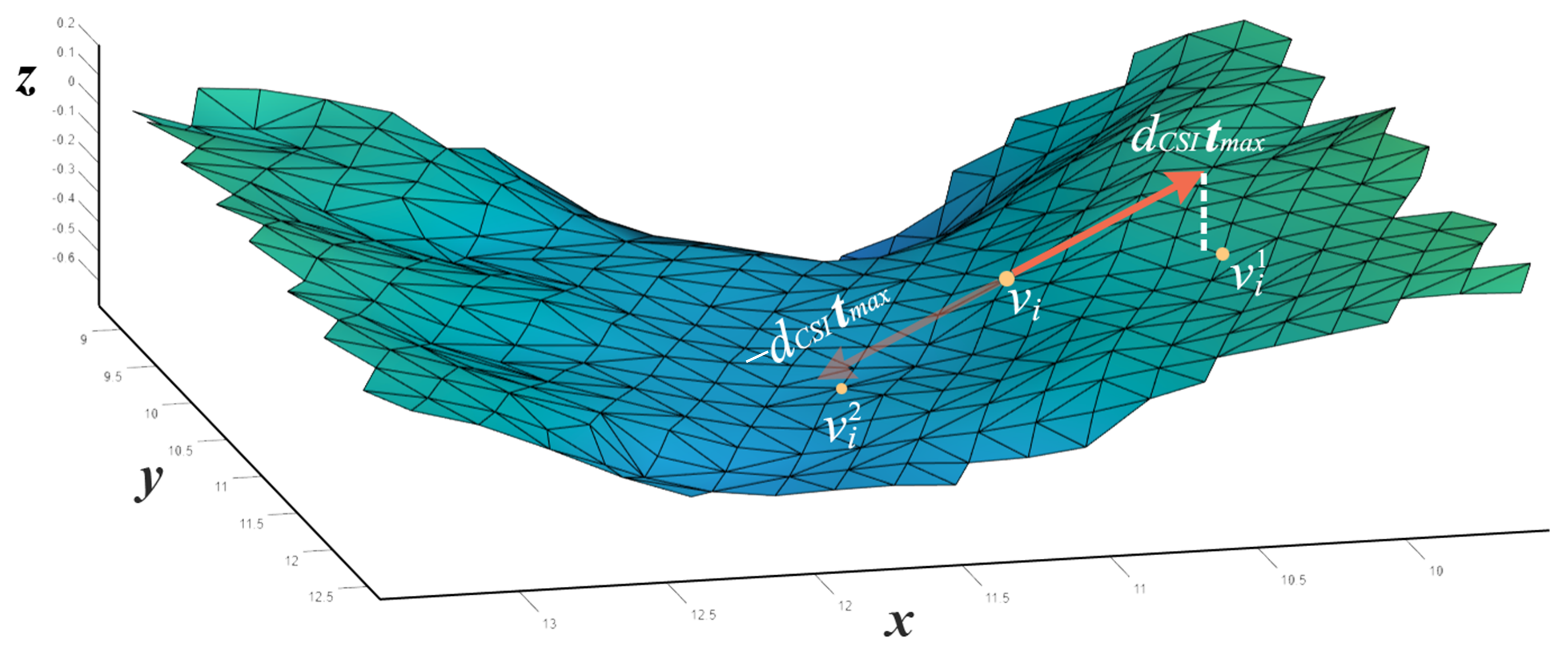
- Relative vertices localization: As mentioned above, to enhance the classification performance at each vertex, the representation of a single SI is augmented with the SIs of its neighboring vertices. To estimate the position of the vertices along the principal curvatures of , the curvature tensors and the curvature derivatives are initially determined, and then the principal curvatures whose directions are denoted by and are obtained [33]. 3D points at a distance of from along , , , and are identified. Since the points are probably not on the mesh surface, we project the 3D points on the mesh and find the vertices closest to the projections. For clarity, we illustrate in Figure 4 how and are searched along the maximal principal direction; the same procedures are repeated in the minimal principal direction to search for and . Once , , , and are determined, the SI information of these surface points and are retrieved from the SI database.
- Sum-pooling: To reduce the dimension of , each SI is subsampled by using a sum-pooling operation with filters and stride s. That is, adjacent bins of the SI are summed up to yield a single bin of the subsampled SI. Therefore, the dimensions of each SI reduces from to . The purpose of this operation is to reduce the size of the SIs while preserving important information before they are vectorized. The sum-pooling operation is inspired by the multi-resolution SI, which applies the concept of pyramid structure of an image to compress a high resolution SI [27]. It is notable that the sum-pooling operation is actually identical to generating SI by partitioning the same 3D space into smaller number of larger subvolumes. In our experiments, s was set to 2.
- Vectorization: This operation converts the original SI information to vector of length for easy merging with the four subsampled SIs. The operation is also repeated for the four subsampled SIs before they are merged. For each of the subsampled SI, the length of the vector is .
- Concatenation: All five vectors obtained from the output of the vectorization stages are concatenated to a single feature vector of length . The concatenated array forms the CSI and it is denoted as .
3.3. Classification
Random forest has been widely and successfully used for various classification problems. We trained a three-class label RF classifier and searched for the optimal set of hyperparameters by varying the number of trees and maximum depth during training. The search for the optimal set of parameters guarantees that the RF model with the best performance is used for the extraction of reliefs from the surface of the stele. The k-NN search algorithm is applied to refine the classification results of the trained RF. The idea of this complementary application is to re-label the surface points by considering the dominant label class of the nearest k neighbors of each vertex. Although the application of k-NN algorithm does not significantly improve the performance of the RF model, it gives a better visualization of the relief, background, and the degraded region. The final result with two classes of the relief and the background is obtained by re-labeling the degraded region class to the background class.
4. Experimental Results and Discussion
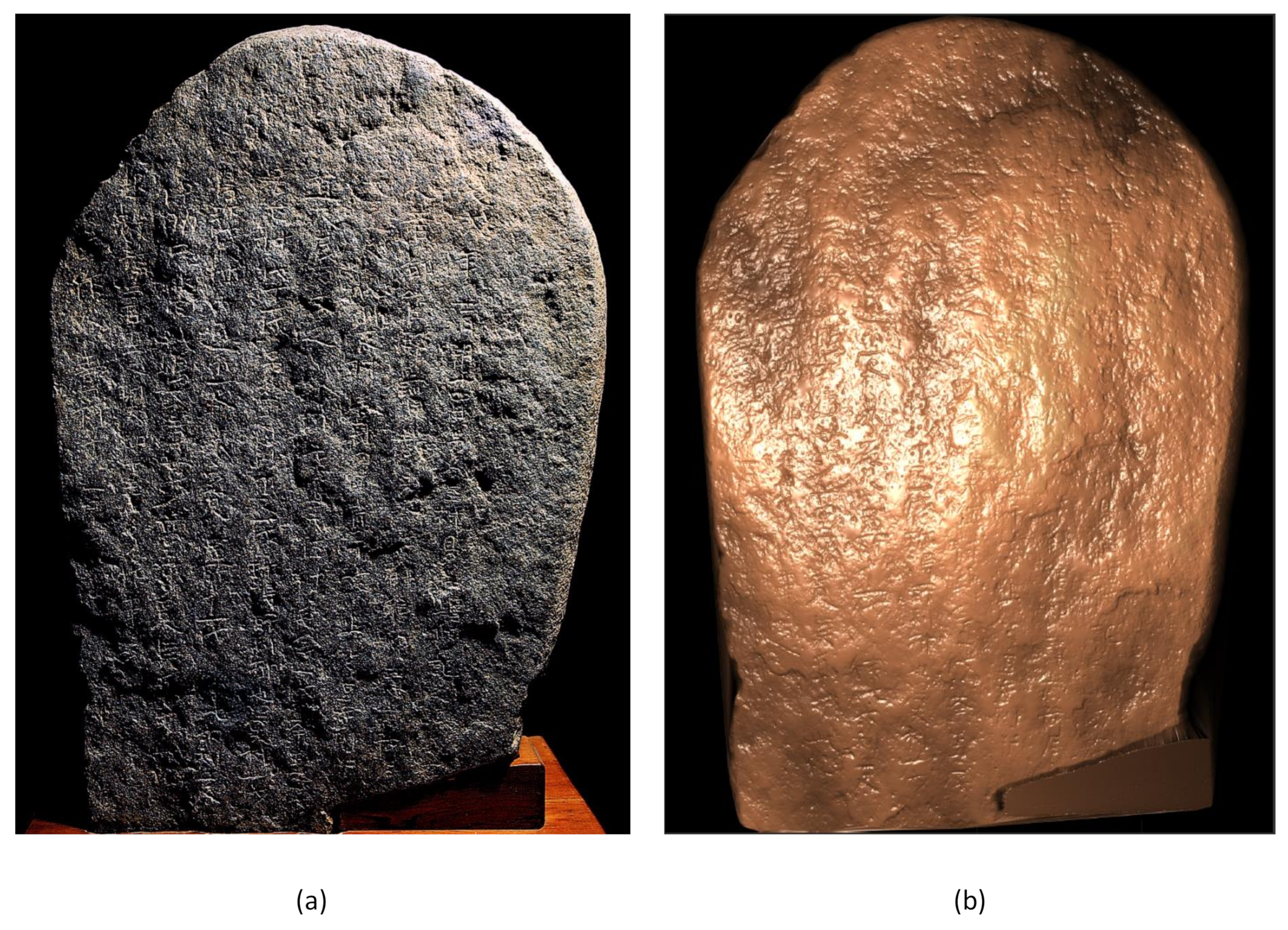
For our experiments, we scanned the stele “Musul-ojakbi” to obtain a 3D mesh with size of mm. The mesh contains over five million vertices, with an average resolution and accuracy of 250 µm and 30 µm, respectively. Musul-ojakbi monument is recorded to have been created in AD 578 during the Silla Dynasty. The monument has a rough surface because it was not ground before engraving and has undergone severe weathering. As illustrated in Figure 5, the characters inscribed on the surface are very difficult to interpret by visual inspection, especially at the center and the lower right portions of the stele. For further information on the Musul-ojakbi stele, we refer the reader to the previous study [24].
To reduce the presence of the degraded region in the ground truth dataset before extracting important features, we carefully cropped fine partitions of the 3D scanned data using the MeshLab 3D processing tool [34]. The ancient stele has 169 partitions containing different characters, but we selected 70 partitions because the reliefs pattern on their surfaces can be traced and labeled as relief, background, or degraded region. The SI and CSI information was extracted per vertex for all the surface points of the 70 partitions. From the information obtained from these 70 partitions, 56 mesh partitions were used for training while 14 partitions for testing. The experiments are presented in the following subsections.
4.1. Hyperparameters Search
We determined the various parameters for the proposed relief extraction method before comparing the performance with existing methods. For clarity, RF models that were trained using the SI and CSI information are denoted as RF(SI) and RF(CSI), respectively.
4.1.1. SI Parameters Search
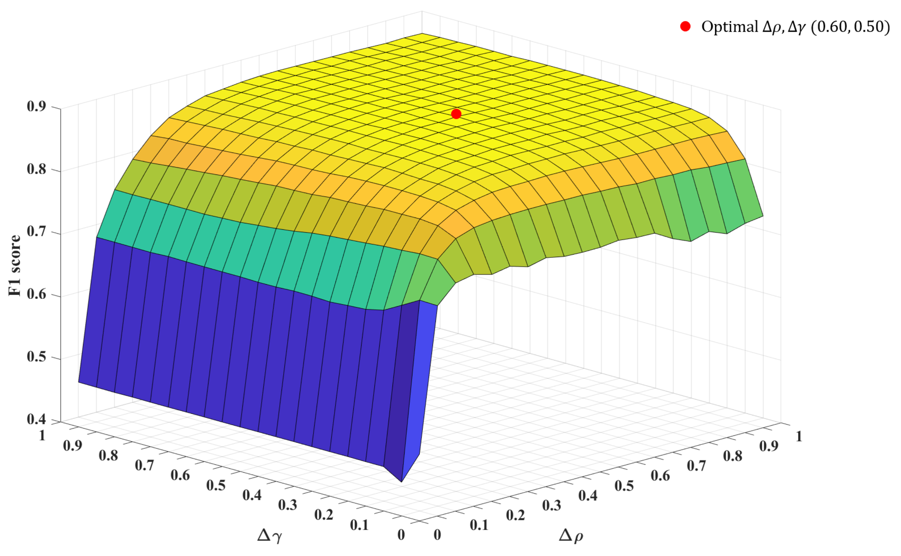
Before generating the CSI, it is important to investigate thoroughly the optimal SI parameter combination. The SI generator requires four parameters: , , , and . In order to limit the feature dimension, and were fixed to 10, resulting in 100 bins of SI. We performed a grid search for and ranging from 0.05 to 1. For fair comparison among different SI combinations, the number of trees and maximum depth for the RF models were initially fixed to 500 and 32, respectively. The F1 scores of the RF models of different SI combinations were compared, as shown by the plot in Figure 6. The plot produces a smooth and concave shape with a peak value of 0.8730 at (, ) = (0.6, 0.5). Since the variation of F1 score is very small when both and are greater than 0.2, the performance of the RF model is insensitive to the SI parameters near the optimal combination. It is noteworthy that the average relief width of the stele is about 2 mm. Since SI of 0.2 and 10 covers a circular area with a radius of 2 mm, it is expected that the SI with a higher contains sufficient information to represent reliefs.
Consequently, other parameter combinations near 0.6 and 0.5 does not reduce the performance much. This SI parameter combination that yielded the highest F1 score of 0.8730 is the optimal.
4.1.2. RF Hyperparameters Search
Following the investigation of the optimal SI parameters, were searched for the RF hyperparameters. Several RF models with different number of trees, , and maximum depth, , were trained with the optimal SI parameter combination, i.e., , , , and selected as 0.6, 0.5, 10, and 10, respectively. The performances of 12 RF models are presented in Table 1. From the search results, the RF model of 1000 trees and maximum depth of 32 performed better than other models in terms of accuracy, F1 score, and recall; however, the precision was slightly lower than 0.8814. Based on these results, the number of trees and maximum depth selected for all subsequent RF models were 1000 and 32, respectively.
4.1.3. Effect of the Smoothing Filter
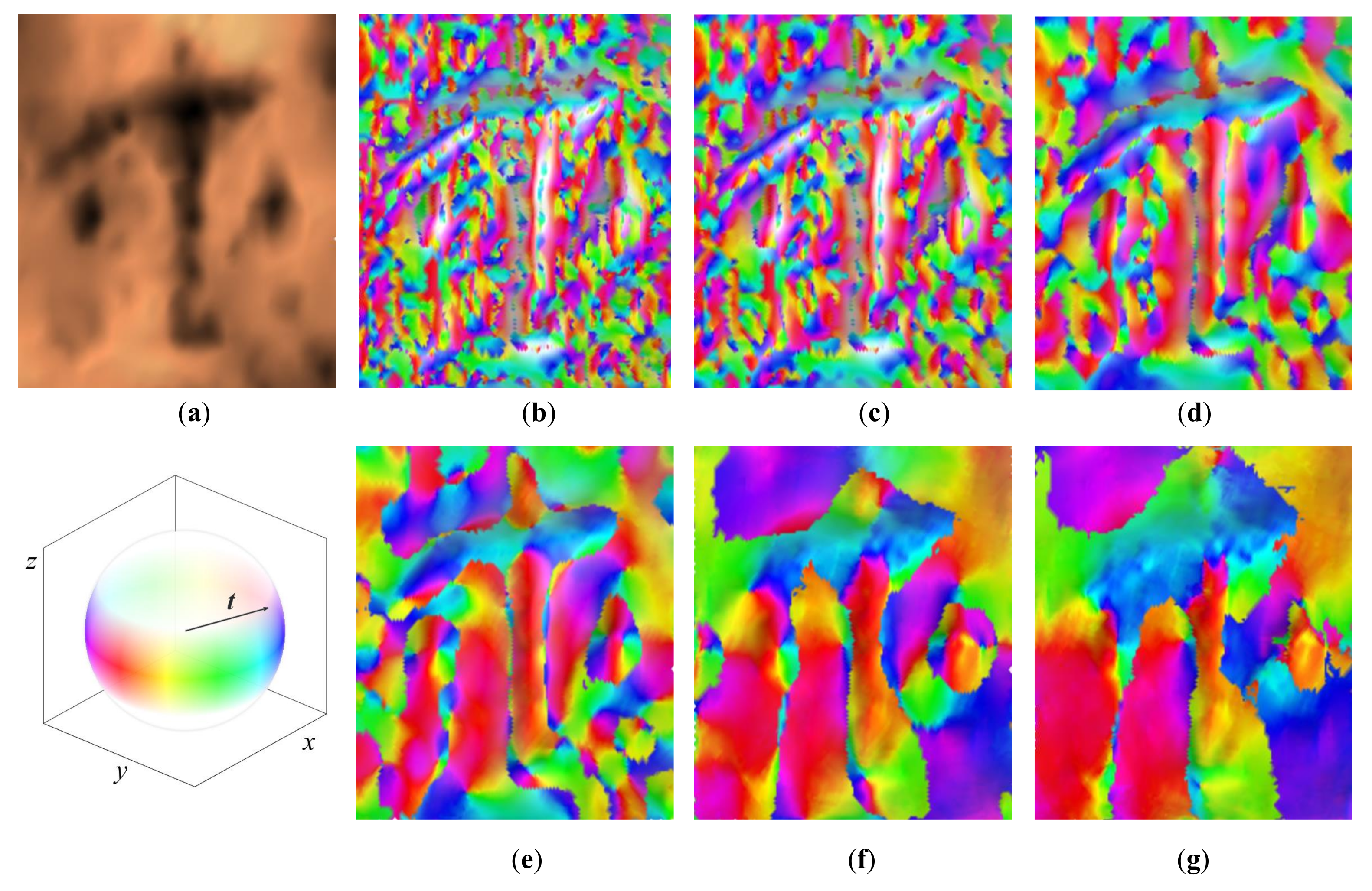
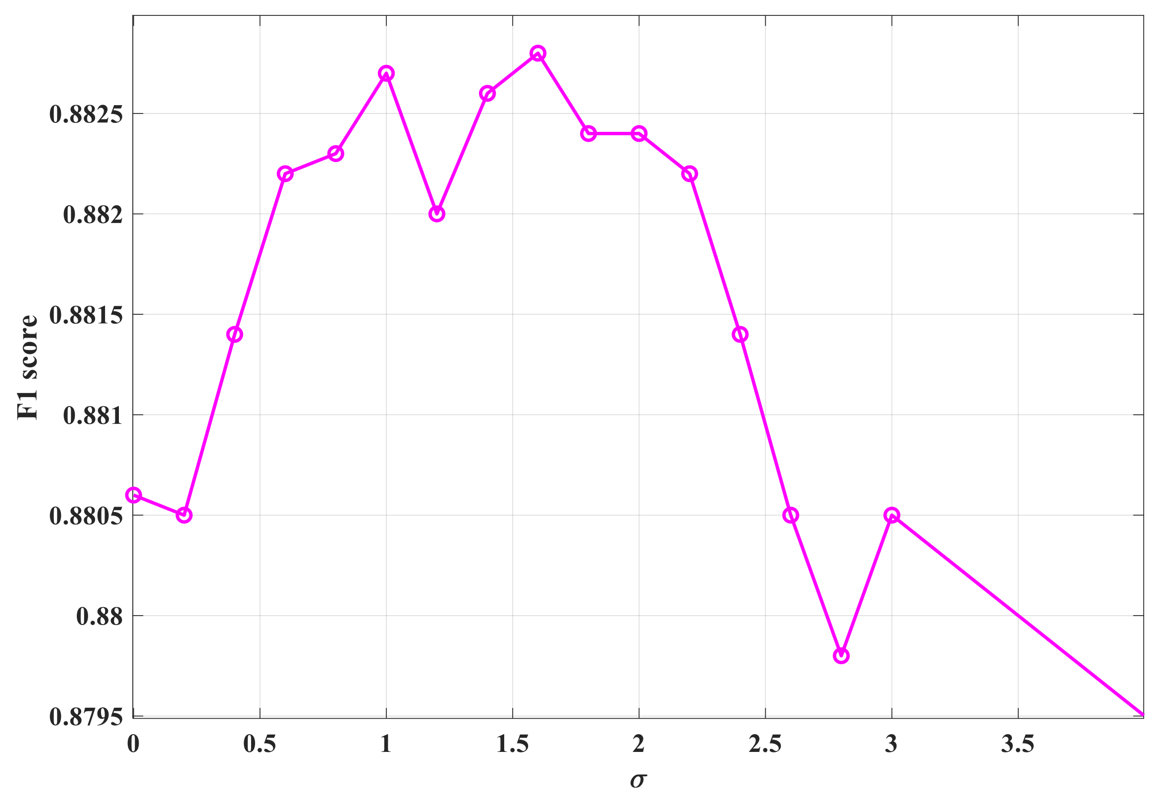
The effect of the Gaussian smoothing on the estimation of curvatures was investigated. Figure 7 illustrates the maximal principal curvature direction of a mesh partition in colors. Hue changes with respect to the azimuthal angle of the curvature direction, while saturation reduces as its elevation angle increases. When the standard deviation of the filter, , is 0.9 and 1.6 (Figure 7d,e), the vertices are realigned such that surfaces with similar principal directions have the same color. At = 4, the principal direction of the vertices are seriously disoriented, and this standard deviation value is not recommended to be used (Figure 7g). Since the estimation of curvatures is directly linked to the localization of the four relative points used in CSI, it is also vital to demonstrate how the variation in affects the extraction of reliefs. For s = 2, the size of the subsampled SI is 5 × 5, and is initially selected as 1. Figure 8 shows that, as the value of increases from 0, the performances of the models also increase up to the highest F1 score of 0.8828. However, after 1.6, the performances of the RF models start to decline. This observation is in line with the colormap of curvature directions reported in Figure 7, in which, when is large, the surface becomes severely flattened and the curvature directions does not provide any useful information. In the proposed method, = 1.6 was used for the Gaussian filter before estimating the principal curvatures of the mesh surface.
4.1.4. Search
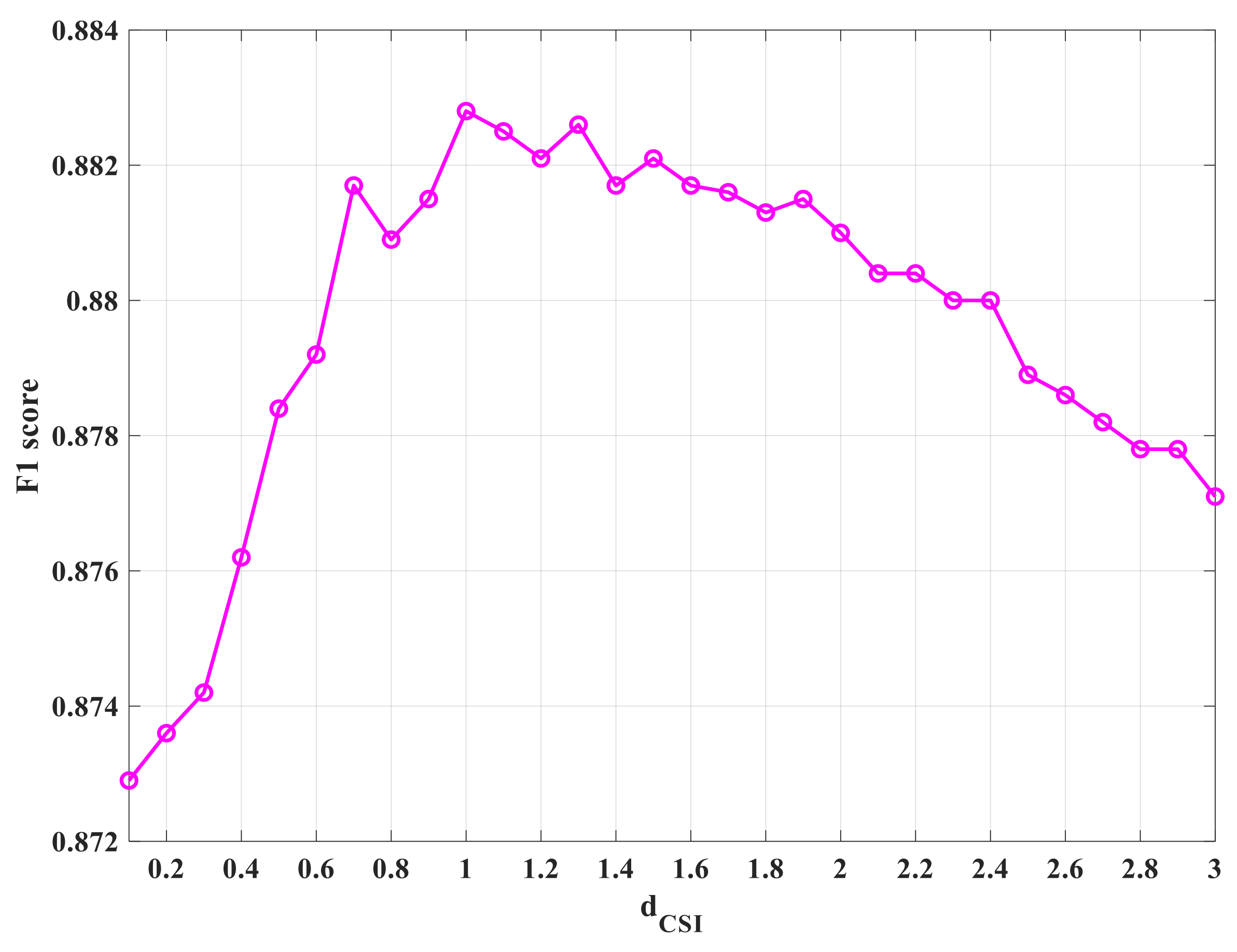
The distance of relative vertices from the reference vertex is also a factor that influences the CSI. Using the parameters of , , , , and as determined, i.e., 0.6, 0.5, 1000, 32, and 1.6, respectively, the performances of several RF models trained using the CSI generated from several values of are illustrated in Figure 9. The plot reveals that, when the value is small, that is, close to zero, the subsampled SI of the relative vertices has similar information as that of the reference vertex. However, as increases, the subsampled SI provides additional information, thereby improving the performance of the RF models in the detection of reliefs. At 2, the performances of the RF models consistently decrease. According to the plot, the RF model with acceptable performance is observed when is 1 with the F1 score of 0.8828.
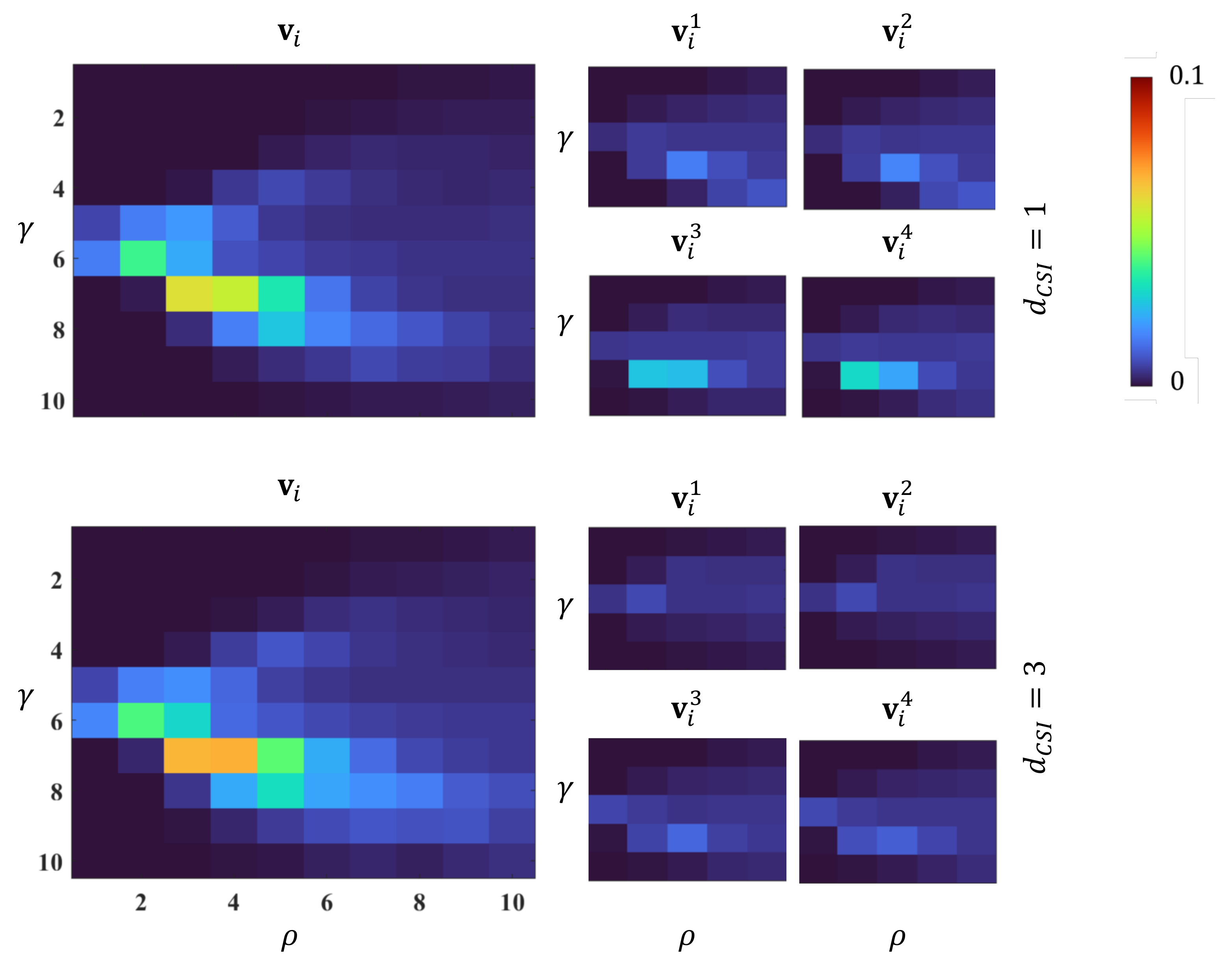
The feature importance of two RF(CSI)s with the same SI parameters (, , , and of 10, 10, 0.6, and 0.5, respectively) but different are compared in Figure 10. The additional information of the relative surface points in RF(CSI) with 1 shows that the model is more descriptive than RF(CSI) of 3. Specifically, the incremental performance is related to the subsampled SI of and searched along the minimal principal direction, . These two relative points contain important features and their uniqueness is what make the model accurately identify relief or non-relief regions. Another interpretation is that, if the reference vertex is in the valley, then and would also be in the valley (within relief).
4.1.5. Size of Neighboring Vertices in k-NN
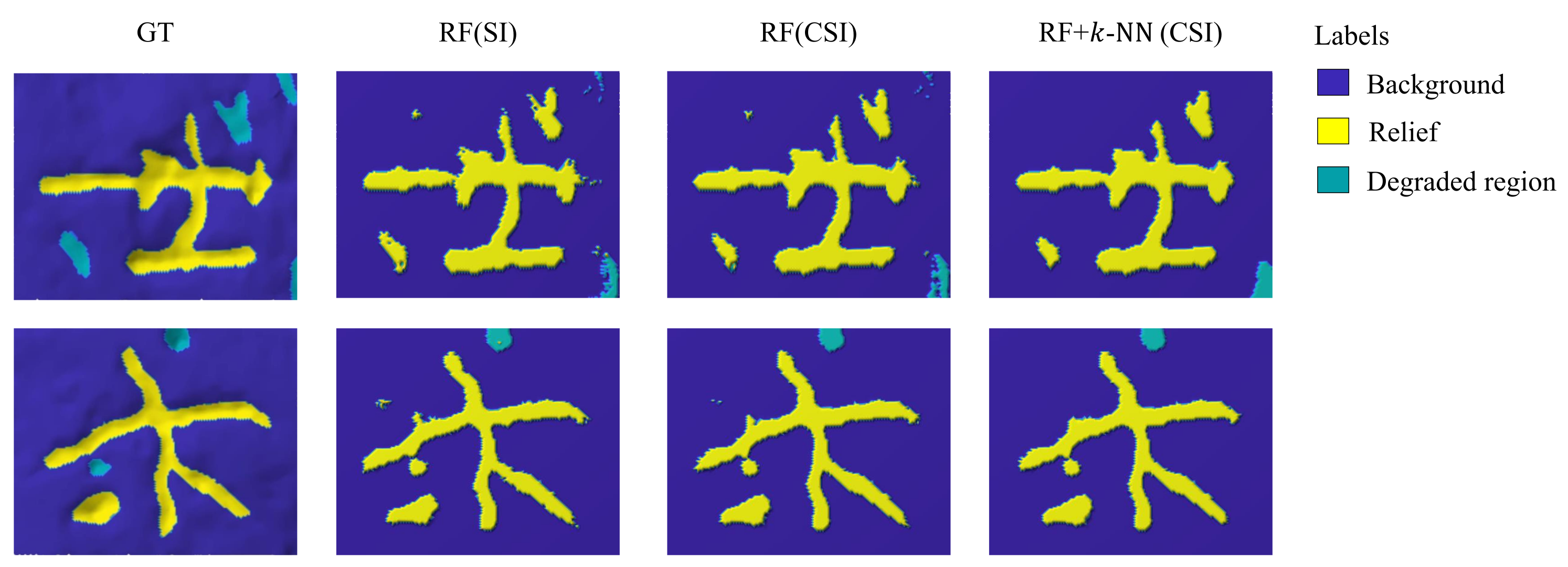
Lastly, we investigated the influence of different k-neighbors in refining the classification results of RF(CSI). Table 2 presents the performance of the RF model with suitable hyperparameters and eight different k sizes. The accuracy and F1 score are highest at 60. Considering the case when 60, the accuracy and F1 score of the classification results are higher than the other cases. Although the application of the k-NN does not significantly improve the result, it provides a good visualization as the relief, background, and degraded region are well clustered, as shown in Figure 11. The second and third columns of Figure 11 were obtained using the RF models trained using SI and CSI, respectively. The fourth column was obtained after applying k-NN to the results in the third column. The k-NN fills the holes and gets rid of isolated points. Once the relief, background, and degraded region are well clustered, it is possible to change the degraded region to the background region, thereby making the classification a two-class label consisting of relief and background regions.
4.2. Effectiveness of the Proposed Method
4.2.1. SI and CSI
In the proposed method, the CSI is geometrically configured by multiple SIs to enhance the surface representation. In order to demonstrate the effectiveness of the CSI, we compared the RF models that were trained using CSI and SI information, respectively. For fair comparison, except feature vectors fed to both the RF models, the identical pipeline, i.e., three-class classifier followed by the k-NN algorithm and re-labeling, was employed. Considering that the dimension of CSI is 200, i.e., = 10 and = 10, the SI of 200 bins was generated using , , , and as 20, 10, 0.3, and 0.5, respectively. Note that 0.3 in the SI of 200 bins to make the spin image coverage area the same as that of CSI in the -direction. Since in SI was doubled, was halved.
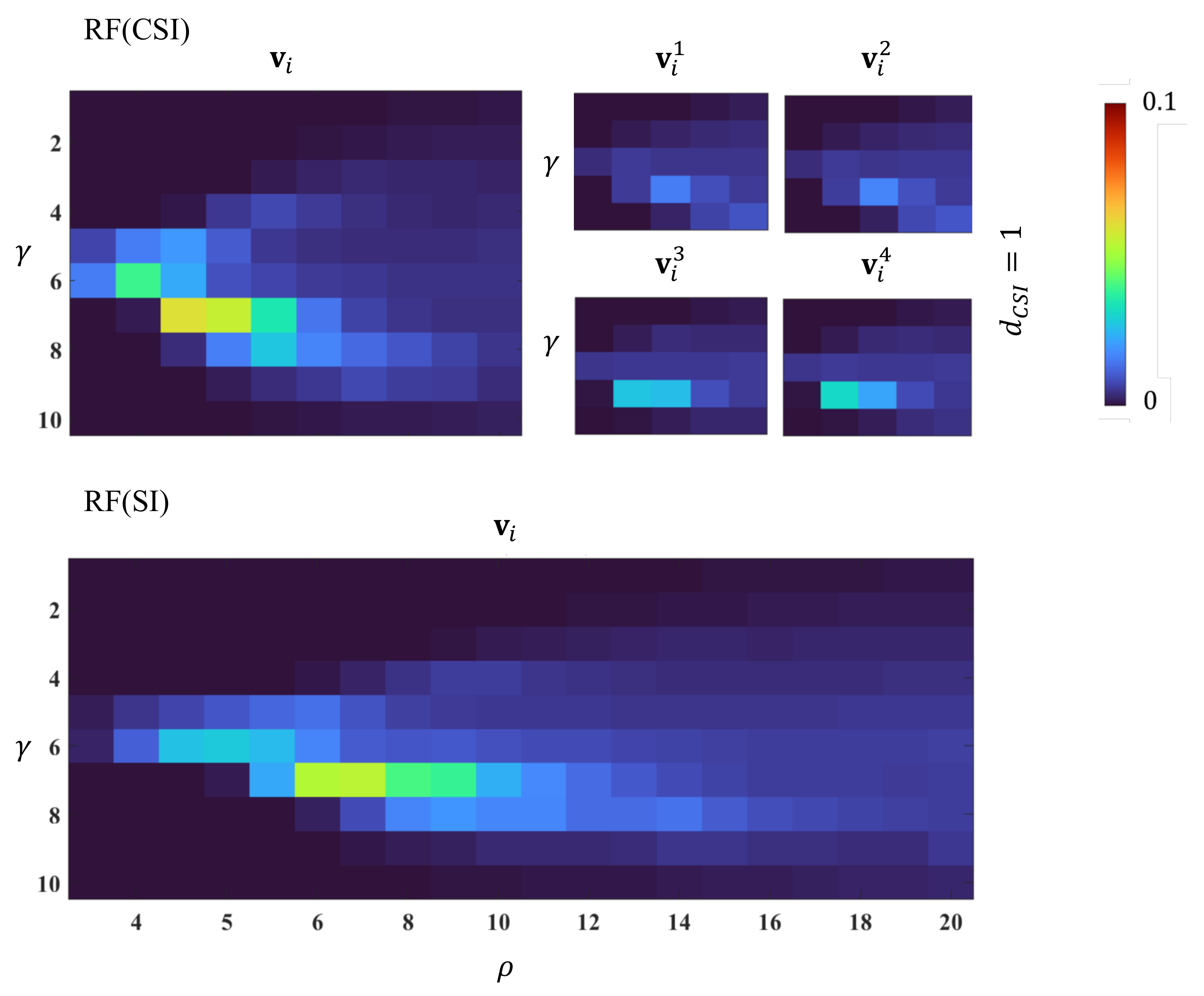
Table 3 shows the performance of the two RF models after applying k-NN. The RF(CSI) has a better performance than the RF(SI) in all metrics. This impressive performance is attributed to the additional features (from the subsampled SI) contained in CSI, which makes the classifier understand the differences between the class labels of the surface regions. The feature importance of the two RF models are illustrated in Figure 12. There are many bins in RF(SI) with less significance compared to RF(CSI). In addition, the important feature bins in RF(SI) are also contained in the feature bins of the RF(CSI), which implies that the original local surface information is preserved in the CSI.
4.2.2. Two-Class and Three-Class RF(CSI)
Another way to verify the effectiveness of the proposed method is to perform a direct two-class relief extraction, i.e., the RF classifier was trained with two classes, relief and background background. The comparison of the classification results between the two-class and three-class RF(CSI) is presented in Table 4. The performance of the three-class RF is higher than the two-class RF in all metrics except precision. Based on this result, the three-class RF(CSI) is more reliable in the extraction of reliefs when compared to the two-class RF(CSI).
4.3. Evaluation of the Proposed Method with Other Existing Methods
In order to evaluate the performance of the proposed method, we compared it with several methods including the height-based method [8], the curvature-based method [7], the modified curvature-based method [18], and the SVM trained on appearance, cross-section, and local extrema-based features [24]. The parameters used in the proposed method and existing methods are given in Table 5.
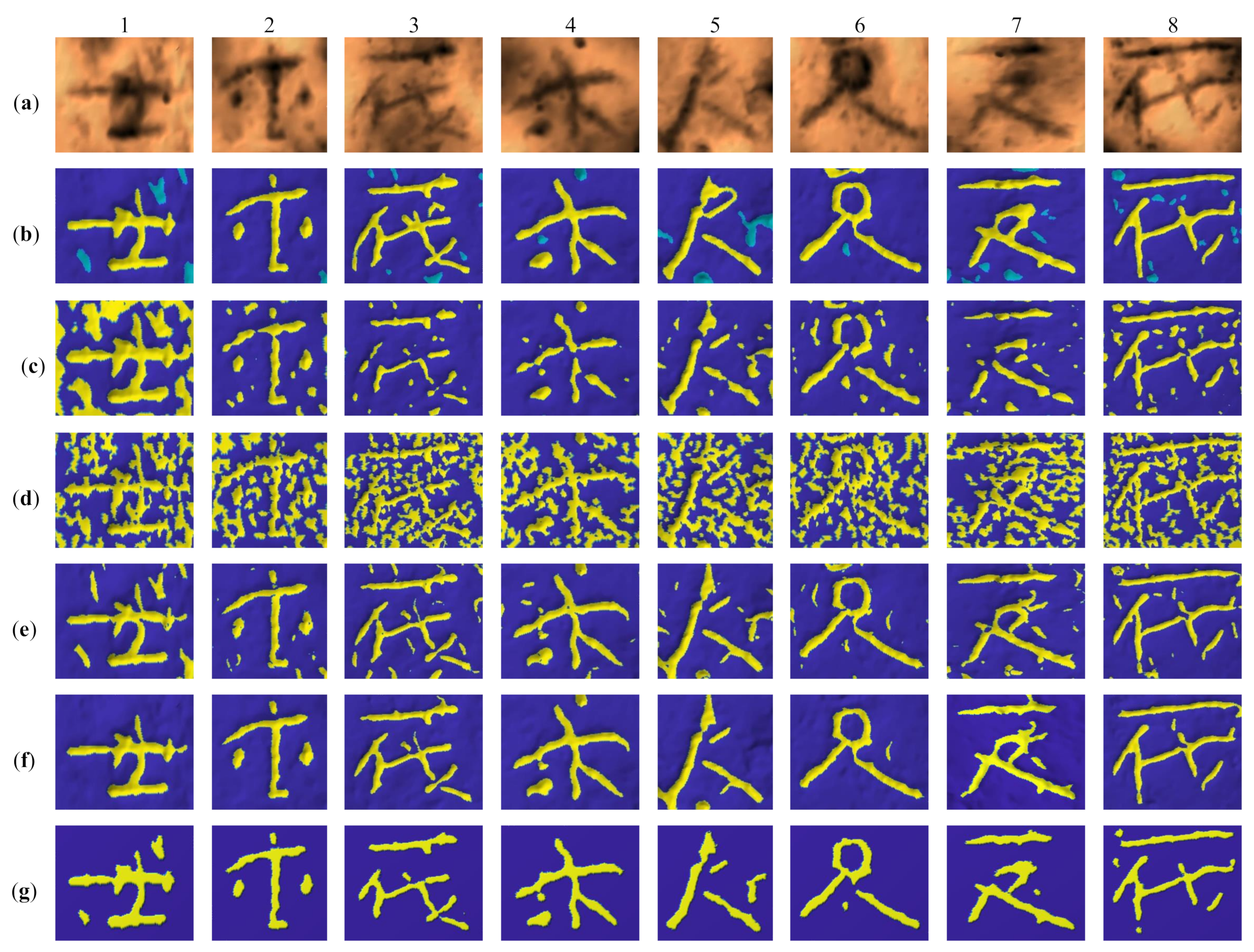
Figure 13a shows eight mesh partitions of the test data and Figure 13b illustrates the corresponding ground truth labels of the mesh partitions with three classes. The degraded region label is utilized in the SVM-based method and the proposed method, while the label is treated as background in the other methods.
As shown in Figure 13c, the height-based method produces unsatisfactory classification results because of the inconsistencies with the distribution of the heights, largely from the degraded region. Figure 13d shows the relief regions extracted using the curvature-based method. The method yields an unreliable extraction of reliefs due to noisy curvatures without the consideration of the rough surface of the stele. Furthermore, the boundaries of the extracted relief regions are not smooth, and it is obvious that the reliefs are not accurately extracted. There is significant improvement in the modified curvature-based method when compared with results from the curvature-based method. However, the modified curvature-based method cannot distinguish degraded region from reliefs, and thus results in many false detections, as shown in Figure 13e.
The machine learning-based methods using SVM and RF are both promising and they outperformed all other methods by eliminating degraded regions (see Figure 13f,g). However, the SVM-based method misclassifies many thin and small degraded regions as reliefs, which hinders recognition of the characters. The proposed method yielded more pleasant results by suppressing those thin degraded regions and producing reliefs with smooth boundaries.
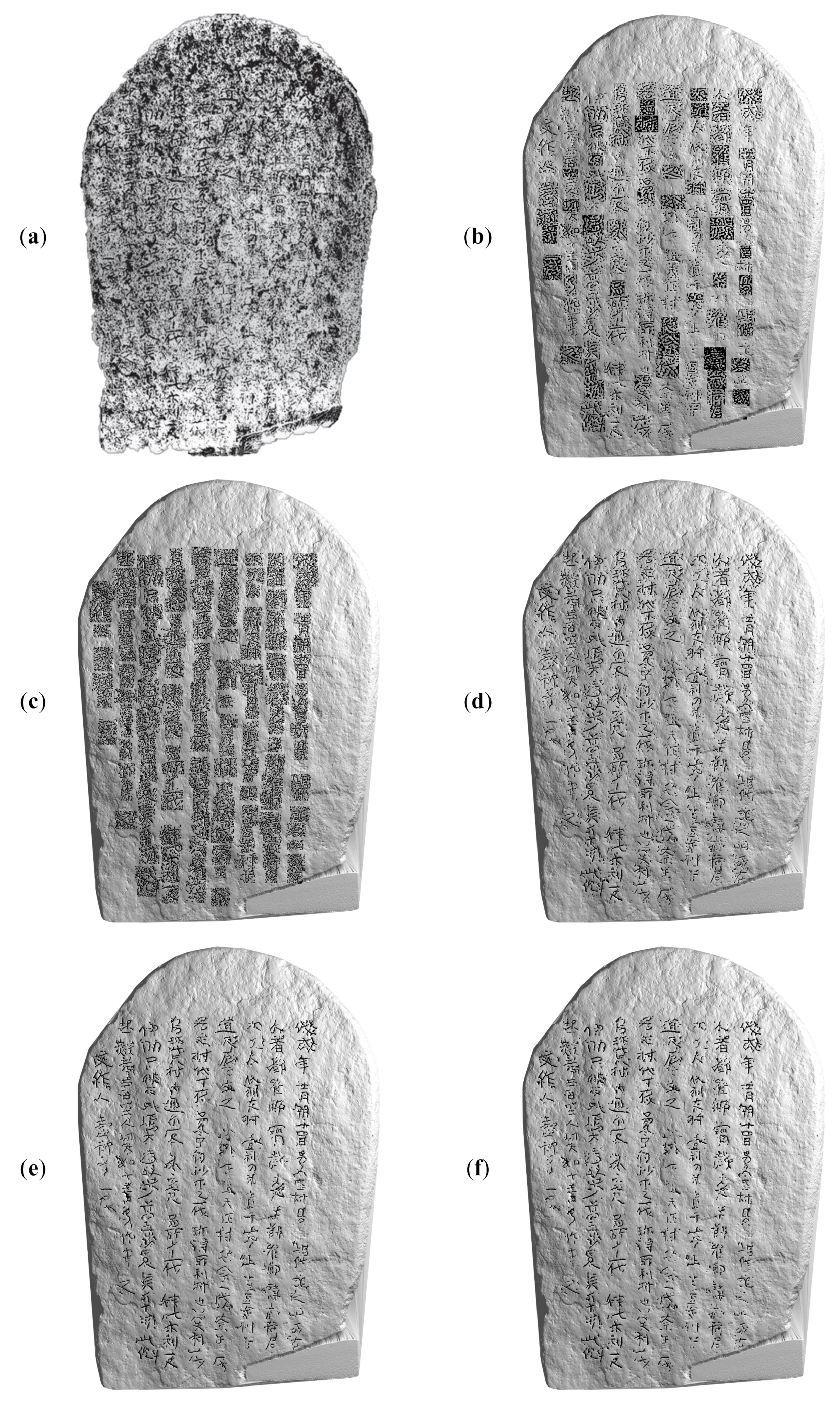
Figure 14 illustrates the results of the comparative methods with respect to the entire ancient stele. The stone rubbing image in Figure 14a indicates not only the reliefs but also cracks and scratches, which makes it difficult for the epigraphists to recognize the characters correctly. The results obtained using the height-based method and the curvature-based method are presented in Figure 14b,c. The classification results are inconsistent as the methods are affected by the degraded regions. There is a significant improvement in the modified curvature-based method, but the extracted reliefs are not accurate and precise (see Figure 14d). For the proposed method, we cross-validated the CSI information by separating the 70 mesh partitions into five folds. Four folds were used to train the RF model in the proposed method and the last fold was selected as test data. This process was repeated until we were able to extract the reliefs for all 70 mesh partitions. One of the RF models trained from the fold was applied to the remaining 113 mesh partitions that were not included in the train. The initial classification result of the 169 mesh partitions were refined with the k-NN, and the result is presented in Figure 14f. The classification result for the SVM-based method in Figure 14e was obtained in the same procedure, but the SVM models were trained using the appearance, cross-section, and local extrema features extracted from the surface of the mesh partitions. From visual inspection, the classification results obtained from the machine learning-based methods involving SVM and RF models were promising when compared to other existing methods, as illustrated in Figure 14e,f. This indicates that the geometrical features extracted in the SVM-based method contained useful information for identifying reliefs and background, and this observation is the same in the proposed RF-based method involving CSI features. It is difficult to quantitatively analyze the performance of these methods on the entire stele because there is no ground truth label for the 113 mesh partitions.
The performance of the machine learning methods, based on SVM and RF (with and without k-NN), were further evaluated using a fold containing the same 14 mesh partitions selected as test data. These machine learning methods were considered for comparison since their classification results are relatively similar. The comparison of the performance of these methods is presented in Table 6. The initial classification result obtained using the proposed method without k-NN, denoted as RF(CSI), is better than the SVM-based method in all metrics except recall. To further improve the reliability of the proposed method, the initial classification results is refined with the k-NN. As such, the proposed method, RF(CSI), refined with k-NN leads the SVM-based method with an increase of approximately , , , and in accuracy, precision, recall, and F1 score, respectively.
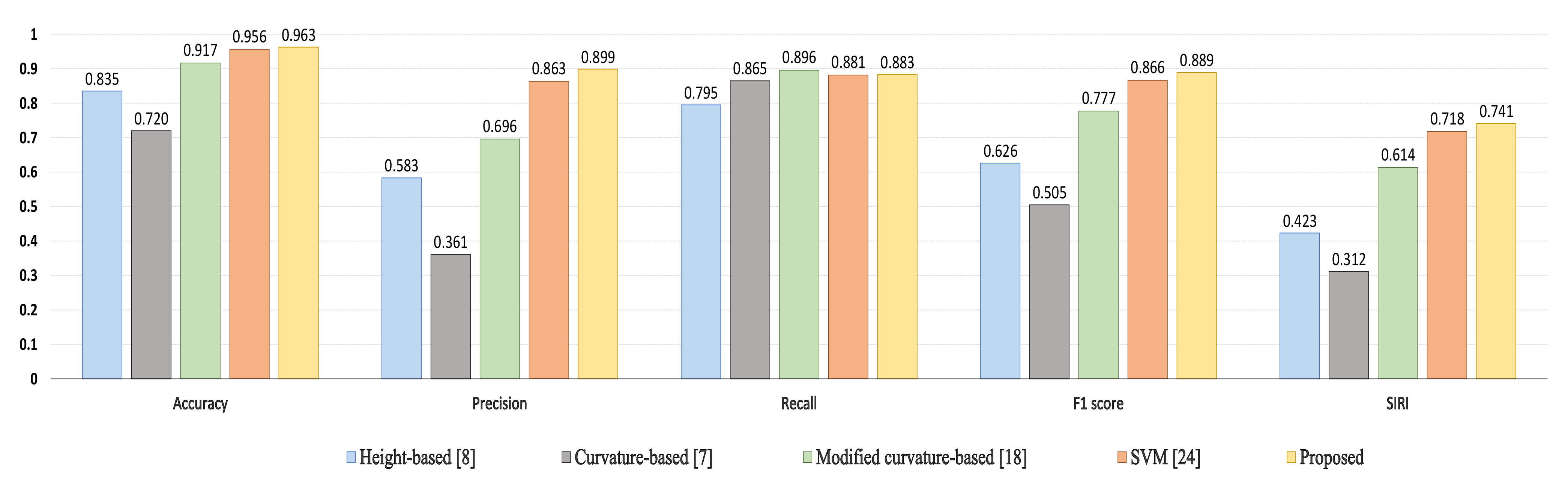
Figure 15 depicts the objective comparison of these methods in terms of accuracy, precision, recall, F1 score, and segmented inscription recognition index (SIRI) [35]. The SIRI can evaluate the inscriptions extracted from the 3D scanning data by imitating human subjective inscription recognition. If a region slightly thinner or thicker than the actual relief segment is detected, it has little effect on the perceived quality of the inscription. In contrast, unexpected misdetection makes the perceived quality degrade significantly. Based on these observations, SIRI evaluates the quality of extracted inscriptions with different importance with respect to region.
For the height-based method, false detection reduces precision and F1 score. The curvature-based method yields a number of false detections, resulting in much lower precision and F1 score. With the modified curvature-based method, all metrics increased but results are not acceptable. The SVM-based method significantly increases in precision, F1 score, and SIRI. The proposed method achieves the highest performance in all metrics except recall. The precision value improves by 0.0353 as compared to the second best method, which also leads to 2.66% higher F1 score. It is noteworthy that the proposed method achieves a larger improvement of 3.2% in SIRI. That indicates that the proposed method produces more recognizable characters, as confirmed in Figure 14f.
5. Conclusions
In this study, we proposed a machine learning-based approach for extracting reliefs from ancient stele. By exploiting the local surface description of the surface of the stele, a cross spin image is used to train a RF model. The optimal parameter combination required for generating the spin image and cross spin image were thoroughly searched. The suitable number of trees and maximum depth for the random forest model were investigated. The initial classification results obtained from the random forest model were refined using k-NN algorithm to cluster regions belonging to the same class label. The degraded regions were identified and re-labeled as background. Experimental results show that the proposed method outperformed previous methods by more than , , , and in accuracy, precision, F1 score, and SIRI, respectively. Especially, the proposed method successfully improved recognizability. With the proposed method, users with little or no experience in epigraphy can accurately identify relief patterns on rough ancient stele.
As part of future work, we would investigate further other advanced machine learning models trained on local surface descriptors, with the objective to improve the classification results, without the need to employ k-NN for refining the results.
Author Contributions
Conceptualization, S.M. and K.-S.C.; methodology, S.M. and K.-S.C.; software, S.M., Y.-C.C., and K.-S.C.; validation, S.M., Y.-C.C., and K.-S.C.; formal analysis, S.M. and K.-S.C.; investigation, S.M.; resources, K.-S.C.; data curation, S.M. and K.-S.C.; writing—original draft preparation, S.M.; writing—review and editing, S.M. and K.-S.C.; visualization, S.M. and K.-S.C.; supervision, K.-S.C.; project administration, K.-S.C.; and funding acquisition, K.-S.C. All authors have read and agreed to the published version of the manuscript.
Funding
This research was supported by Basic Science Research Program through the National Research Foundation of Korea (NRF) funded by the Ministry of Education (2019R1I1A3A01060600). This work was supported by the BK-21 four program through National Research Foundation of Korea (NRF) under Ministry of Education.
Institutional Review Board Statement
Not applicable.
Informed Consent Statement
Not applicable.
Data Availability Statement
Not applicable.
Conflicts of Interest
The authors declare no conflict of interest.
Abbreviations
The following abbreviations are used in this manuscript:
| CSI | Cross spin image |
| k-NN | k-nearest neighbor |
| RF | Random forest |
| SI | Spin image |
| SIRI | Segmented inscription recognition index |
| SVM | Support vector machine |
References
- Johnson, N. Cast in Stone: Monuments, Geography, and Nationalism. Environ. Plan. Soc. Space 1995, 13, 51–65. [Google Scholar] [CrossRef]
- Fitzner, B.; Heinrichs, K. Damage diagnosis at stone monuments-weathering forms, damage categories and damage indices. Acta Univ. Carol. Geol. 2001, 1, 12–13. [Google Scholar]
- Camuffo, D. Physical weathering of stones. Sci. Total. Environ. 1995, 167, 1–14. [Google Scholar] [CrossRef]
- Wikipedia Contributors. Wikipedia. Available online: Https://en.wikipedia.org/wiki/Stone-rubbing (accessed on 18 March 2021).
- Defrasne, C. Digital image enhancement for recording rupestrian engravings: Applications to an alpine rockshelter. J. Archaeol. Sci. 2014, 50, 31–38. [Google Scholar] [CrossRef]
- Kolomenkin, M.; Shimshoni, I.; Tal, A. Prominent field for shape processing and analysis of archaeological artifacts. Int. J. Comp. Vis. 2011, 94, 89–100. [Google Scholar] [CrossRef] [Green Version]
- Lawonn, K.; Trostmann, E.; Preim, B.; Hildebrandt, K. Visualization and extraction of carvings for heritage conservation. IEEE Trans. Vis. Comput. Graph. 2016, 23, 801–810. [Google Scholar] [CrossRef] [PubMed] [Green Version]
- Zatzarinni, R.; Tal, A.; Shamir, A. Relief analysis and extraction. ACM Trans. Graph. (TOG) 2009, 28, 1–9. [Google Scholar] [CrossRef]
- Torrente, M.L.; Biasotti, S.; Falcidieno, B. Recognition of feature curves on 3D shapes using an algebraic approach to Hough transforms. Pattern Recognit. 2018, 73, 111–130. [Google Scholar] [CrossRef] [Green Version]
- Romanengo, C.; Biasotti, S.; Falcidieno, B. Recognising decorations in archaeological finds through the analysis of characteristic curves on 3D models. Pattern Recognit. Lett. 2020, 131, 405–412. [Google Scholar] [CrossRef]
- Harman, J. Using decorrelation stretch to enhance rock art images. In Proceedings of the American Rock Art Research Association Annual Meeting, Sparks, NV, USA, 28–30 May 2005; Volume 28. [Google Scholar]
- Gomes, L.; Regina Pereira Bellon, O.; Silva, L. 3D reconstruction methods for digital preservation of cultural heritage: A survey. Pattern Recognit. Lett. 2014, 50, 3–14. [Google Scholar] [CrossRef]
- Liu, S.; Martin, R.R.; Langbein, F.C.; Rosin, P.L. Segmenting periodic reliefs on triangle meshes. In IMA International Conference on Mathematics of Surfaces; Springer: Berlin/Heidelberg, Germany, 2007; pp. 290–306. [Google Scholar]
- Anderson, S.; Levoy, M. Unwrapping and visualizing cuneiform tablets. IEEE Comput. Graph. Appl. 2002, 22, 82–88. [Google Scholar] [CrossRef]
- Pan, R.; Tang, Z.; Da, W. Digital stone rubbing from 3D models. J. Cult. Herit. 2019, 37, 192–198. [Google Scholar] [CrossRef]
- Weyrich, T.; Pauly, M.; Keiser, R.; Heinzle, S.; Scandella, S.; Gross, M.H. Post-processing of scanned 3D surface data. In Proceedings of the First Eurographics Conference on Point-Based Graphics, Zurich, Switzerland, 2–4 June 2004; pp. 85–94. [Google Scholar]
- Frangi, A.F.; Niessen, W.J.; Vincken, K.L.; Viergever, M.A. Multiscale vessel enhancement filtering. In International Conference on Medical Image Computing and Computer-Assisted Intervention; Springer: Berlin/Heidelberg, Germany, 1998; pp. 130–137. [Google Scholar]
- Heo, E.J.; Sa, J.M.; Choi, K.S. Relief extraction from stone monuments. IEIE Trans. Smart Process. Comput. 2018, 7, 321–324. [Google Scholar] [CrossRef]
- Fiorucci, M.; Khoroshiltseva, M.; Pontil, M.; Traviglia, A.; Del Bue, A.; James, S. Machine learning for cultural heritage: A survey. Pattern Recognit. Lett. 2020, 133, 102–108. [Google Scholar] [CrossRef]
- Grilli, E.; Remondino, F. Classification of 3D Digital Heritage. Remote Sens. 2019, 11, 847. [Google Scholar] [CrossRef] [Green Version]
- Belhi, A.; Bouras, A.; Al-Ali, A.K.; Foufou, S. A machine learning framework for enhancing digital experiences in cultural heritage. J. Enterp. Inf. Manag. 2020. [Google Scholar] [CrossRef]
- Liu, S.; Martin, R.R.; Langbein, F.C.; Rosin, P.L. Background surface estimation for reverse engineering of reliefs. Int. J. CAD/CAM. 2007, 7, 31–40. [Google Scholar]
- Zeppelzauer, M.; Poier, G.; Seidl, M.; Reinbacher, C.; Schulter, S.; Breiteneder, C.; Bischof, H. Interactive 3D segmentation of rock-art by enhanced depth maps and gradient preserving regularization. J. Comput. Cult. Herit. (JOCCH) 2016, 9, 1–30. [Google Scholar] [CrossRef]
- Choi, Y.C.; Murtala, S.; Jeong, B.C.; Choi, K.S. Relief Extraction from a Rough Stele Surface using SVM-based Relief Segment Selection. IEEE Access. 2021, 9, 4973–4982. [Google Scholar] [CrossRef]
- Johnson, A.E. Spin-Images: A Representation for 3-D Surface Matching. Ph.D. Dissertation, The Robotics Institute, Carnegie Mellon University, Pittsburgh, PA, USA, 1997. [Google Scholar]
- Park, D.R.; Choi, K.S. A technique for extracting 3D tombstone carvings using spin images. J. Inst. Electron. Eng. 2019, 56, 52–59. [Google Scholar]
- Dinh, H.Q.; Kropac, S. Multi-Resolution Spin-Images. In Proceedings of the IEEE Computer Society Conference on Computer Vision and Pattern Recognition (CVPR’06), New York, NY, USA, 17 June 2006; Volume 1, pp. 863–870. [Google Scholar]
- Belongie, S.; Malik, J.; Puzicha, J. Shape context: A new descriptor for shape matching and object recognition. In Advances in Neural Information Processing Systems; Leen, T.K., Dietterich, T.G., Tresp, V., Eds.; MIT Press: Cambridge, MA, USA, 2001; pp. 831–837. [Google Scholar]
- Tombari, F.; Salti, S.; Di Stefano, L. Unique shape context for 3D data description. In Proceedings of the ACM Workshop on 3D Object Retrieval (3DOR ’10), Firenze, Italy, 25 October 2010; Association for Computing Machinery: New York, NY, USA, 2010; pp. 57–62. [Google Scholar]
- Belongie, S.; Malik, J.; Puzicha, J. Shape matching and object recognition using shape contexts. IEEE Trans. Pattern Anal. Mach. Intell. 2002, 24, 509–522. [Google Scholar] [CrossRef] [Green Version]
- Mikolajczyk, K.; Schmid, C. A performance evaluation of local descriptors. IEEE Trans. Pattern Anal. Mach. Intell. 2005, 27, 1615–1630. [Google Scholar] [CrossRef] [PubMed] [Green Version]
- Choi, K.-S.; Kim, D.-H. Angular-partitioned spin image descriptor for robust 3D facial landmark detection. Electron. Lett. 2013, 49, 1454–1455. [Google Scholar] [CrossRef]
- Rusinkiewicz, S. Estimating curvatures and their derivatives on triangle meshes. In Proceedings of the 2nd International Symposium on 3D Data Processing, Visualization and Transmission 3DPVT 2004, Thessaloniki, Greece, 9 September 2004; pp. 486–493. [Google Scholar]
- Cignoni, P.; Callieri, M.; Corsini, M.; Dellepiane, M.; Ganovelli, F.; Ranzuglia, G. MeshLab: An Open-Source Mesh Processing Tool. In Proceedings of the Eurographics Italian Chapter Conference, Salerno, Italy, 2–4 July 2008; pp. 129–136. [Google Scholar]
- Jeong, B.-C.; Choi, Y.-C.; Murtala, S.; Choi, K.-S. Segmented inscription recognition index for measuring the inscription quality extracted from 3-D data. IEIE Trans. Smart Process. Comput. 2020, 9, 445–451. [Google Scholar] [CrossRef]
Figure 1.
SI representation for a reference oriented point (, ): (a) 3D point cloud and an imaginary plane P containing and having the normal, ; (b) the 3D space around is partitioned into non-overlapping subspaces; and (c) the 2D histogram of the spin image with axes and .
Figure 1.
SI representation for a reference oriented point (, ): (a) 3D point cloud and an imaginary plane P containing and having the normal, ; (b) the 3D space around is partitioned into non-overlapping subspaces; and (c) the 2D histogram of the spin image with axes and .

Figure 2.
The proposed relief extraction method.

Figure 3.
Offline SI generation and storage.

Figure 4.
Relative vertices localization. For , a 3D point located at a distance of in direction is identified. The 3D point is projected on the mesh and the closest vertex is obtained as the relative vertex . Similarly, is identified using the opposite direction of .
Figure 4.
Relative vertices localization. For , a 3D point located at a distance of in direction is identified. The 3D point is projected on the mesh and the closest vertex is obtained as the relative vertex . Similarly, is identified using the opposite direction of .

Figure 5.
Musul-ojakbi stele: (a) 2D photograph; and (b) 3D scanned data.

Figure 6.
The performance of SI-based RF models for different SI parameter combinations ( and ). Both and were set to 10. Each RF model was trained with 500 trees and maximum depth of 32. The best SI parameter combination is (, ) = (0.60, 0.50).
Figure 6.
The performance of SI-based RF models for different SI parameter combinations ( and ). Both and were set to 10. Each RF model was trained with 500 trees and maximum depth of 32. The best SI parameter combination is (, ) = (0.60, 0.50).

Figure 7.
Effects of mesh smoothing on reliability of estimated curvature: (a) mesh partition; (b) no filtering; (c) = 0.3; (d) = 0.9; (e) = 1.6; (f) = 2.0; and (g) = 4.0.
Figure 7.
Effects of mesh smoothing on reliability of estimated curvature: (a) mesh partition; (b) no filtering; (c) = 0.3; (d) = 0.9; (e) = 1.6; (f) = 2.0; and (g) = 4.0.

Figure 8.
Performance of RF models (in terms of F1 score) under different values.

Figure 9.
Performance of RF models (in terms of F1 score) for various values.

Figure 10.
Feature importance of RF (CSI) models 1 and 3.

Figure 11.
Subjective comparison of the classification results before re-labeling. The second and third columns were obtained using the RF models trained using SI and CSI, respectively. The fourth column was obtained after applying k-NN to the third column. The k-NN fills the holes and gets rid of isolated points.

Figure 12.
Comparison of feature importance of RF(CSI) and RF(SI).

Figure 13.
The comparison of the proposed method and existing methods: (a) mesh partitions; (b) ground truth; (c) the height-based method [8]; (d) the curvature-based method [7]; (e) the modified curvature-based method [18]; and (f) the SVM-based method [24]. (g) The proposed method.

Figure 14.
The comparison of the existing relief extraction methods and the proposed method: (a) stone rubbing; (b) the height-based method [8]; (c) the curvature-based method [7]; (d) the modified curvature-based method [18]; (e) the SVM-based method [24]; and (f) the proposed method.

Figure 15.
Performance evaluation of the relief extraction methods in terms of precision, accuracy, recall, F1 score, and SIRI.
Figure 15.
Performance evaluation of the relief extraction methods in terms of precision, accuracy, recall, F1 score, and SIRI.


Table 1.
Search for suitable number of trees and maximum depth for RF.
| Trees () | Max. Depth () | Accuracy | Precision | Recall | F1 Score |
|---|---|---|---|---|---|
| 200 | 16 | 0.9548 | 0.8755 | 0.8628 | 0.8691 |
| 200 | 32 | 0.9560 | 0.8808 | 0.8636 | 0.8721 |
| 200 | 64 | 0.9559 | 0.8811 | 0.8631 | 0.8720 |
| 500 | 16 | 0.9549 | 0.8755 | 0.8632 | 0.8693 |
| 500 | 32 | 0.9562 | 0.8810 | 0.8651 | 0.8730 |
| 500 | 64 | 0.9562 | 0.8814 | 0.8646 | 0.8729 |
| 1000 | 16 | 0.9549 | 0.8756 | 0.8635 | 0.8695 |
| 1000 | 32 | 0.9562 | 0.8808 | 0.8655 | 0.8731 |
| 1000 | 64 | 0.9562 | 0.8813 | 0.8642 | 0.8728 |
| 1500 | 16 | 0.9550 | 0.8756 | 0.8637 | 0.8696 |
| 1500 | 32 | 0.9562 | 0.8809 | 0.8649 | 0.8728 |
| 1500 | 64 | 0.9561 | 0.8812 | 0.8642 | 0.8726 |
Table 2.
Search for acceptable size of k.
| k | Accuracy | Precision | Recall | F1 Score |
|---|---|---|---|---|
| 10 | 0.9610 | 0.8907 | 0.8836 | 0.8851 |
| 20 | 0.9612 | 0.8921 | 0.8839 | 0.8860 |
| 30 | 0.9615 | 0.8929 | 0.8843 | 0.8866 |
| 40 | 0.9619 | 0.8944 | 0.8846 | 0.8875 |
| 50 | 0.9622 | 0.8959 | 0.8848 | 0.8883 |
| 60 | 0.9625 | 0.8985 | 0.8832 | 0.8889 |
| 70 | 0.9623 | 0.9006 | 0.8793 | 0.8880 |
| 80 | 0.9622 | 0.9026 | 0.8757 | 0.8873 |
Table 3.
Comparison of the representation performance of SI and CSI. The dimension of both SI and CSI feature vectors is 200.
Table 3.
Comparison of the representation performance of SI and CSI. The dimension of both SI and CSI feature vectors is 200.
| Metrics | Using SI | Using CSI |
|---|---|---|
| Accuracy | 0.9594 | 0.9625 |
| Precision | 0.8914 | 0.8985 |
| Recall | 0.8716 | 0.8832 |
| F1 score | 0.8796 | 0.8889 |
Table 4.
Comparison of the two-class and three-class RF(CSI). and are 1000 and 32 in both models.
| Metrics | Two-Class | Three-Class |
|---|---|---|
| Accuracy | 0.9606 | 0.9625 |
| Precision | 0.9120 | 0.8985 |
| Recall | 0.8557 | 0.8832 |
| F1 score | 0.8810 | 0.8889 |
Table 5.
Summary of parameters for comparative methods.
| Proposed | Curvature-Based [7,18] | ||||
|---|---|---|---|---|---|
| CSI | RF | 0.7 | |||
| 0.6 | 1000 | 0.1 | |||
| 0.5 | 32 | ||||
| 10 | |||||
| 10 | |||||
| 1.6 | |||||
| 1 | |||||
| s | 2 | ||||
Table 6.
Comparative performance of machine learning methods.
| Method | Accuracy | Precision | Recall | F1 Score |
|---|---|---|---|---|
| SVM | 0.9557 | 0.8632 | 0.8814 | 0.8664 |
| RF(CSI) | 0.9596 | 0.8914 | 0.8744 | 0.8828 |
| RF(CSI), k-NN | 0.9625 | 0.8985 | 0.8832 | 0.8889 |
Publisher’s Note: MDPI stays neutral with regard to jurisdictional claims in published maps and institutional affiliations. |
© 2021 by the authors. Licensee MDPI, Basel, Switzerland. This article is an open access article distributed under the terms and conditions of the Creative Commons Attribution (CC BY) license (https://creativecommons.org/licenses/by/4.0/).
Share and Cite
MDPI and ACS Style
Murtala, S.; Choi, Y.-C.; Choi, K.-S. A Machine Learning Method Based on 3D Local Surface Representation for Recognizing the Inscriptions on Ancient Stele. Appl. Sci. 2021, 11, 5758. https://0-doi-org.brum.beds.ac.uk/10.3390/app11125758
AMA Style
Murtala S, Choi Y-C, Choi K-S. A Machine Learning Method Based on 3D Local Surface Representation for Recognizing the Inscriptions on Ancient Stele. Applied Sciences. 2021; 11(12):5758. https://0-doi-org.brum.beds.ac.uk/10.3390/app11125758
Chicago/Turabian StyleMurtala, Sheriff, Ye-Chan Choi, and Kang-Sun Choi. 2021. "A Machine Learning Method Based on 3D Local Surface Representation for Recognizing the Inscriptions on Ancient Stele" Applied Sciences 11, no. 12: 5758. https://0-doi-org.brum.beds.ac.uk/10.3390/app11125758
Note that from the first issue of 2016, this journal uses article numbers instead of page numbers. See further details here.