A Survey on Change Detection and Time Series Analysis with Applications

Abstract

With the advent of the digital computer, time series analysis has gained wide attention and is being applied to many fields of science. This paper reviews many traditional and recent techniques for time series analysis and change detection, including spectral and wavelet analyses with their advantages and weaknesses. First, Fourier and least-squares-based spectral analysis methods and spectral leakage attenuation methods are reviewed. Second, several time-frequency decomposition methods are described in detail. Third, several change or breakpoints detection methods are briefly reviewed. Finally, some of the applications of the methods in various fields, such as geodesy, geophysics, remote sensing, astronomy, hydrology, finance, and medicine, are listed in a table. The main focus of this paper is reviewing the most recent methods for analyzing non-stationary time series that may not be sampled at equally spaced time intervals without the need for any interpolation prior to the analysis. Understanding the methods presented herein is worthwhile to further develop and apply them for unraveling our universe.

1. Introduction

A periodic oscillation can be described by a smooth sinusoidal function. It may be a function of time or distance. Consider the sinusoidal wave $f\left(t\right)=Asin(2\pi \omega t+\theta )$, where f is a function of time t. The parameters A, $\omega$ and $\theta$ are called the amplitude, cyclic frequency or number of cycles per unit time and phase of the sinusoid, respectively. This function is periodic with period $T=1/\omega$ [1,2]. A time series is an ordered sequence of data points measured at discrete time intervals that may not be equally spaced or may contain data gaps, and so the time series is unequally spaced or unevenly sampled. In certain experiments, measurements may also have uncertainties introduced by random noise and thus may also be unequally weighted [3,4].

In many areas of research, such as geodesy, geophysics, geodynamics, astronomy and speech communications, researchers deal with series of data points measured over time or distance to study the periodicity and/or power of certain constituents. For example, in a speech record, one may be interested in certain signals in the record, such as the voice of a person obscured by other simultaneously recorded constituents, noise from musical instruments and the environment. It is often difficult to study these signals by direct analysis of the time series; however, decomposing the time series into another domain may result in detecting the constituents of interest much easier. Furthermore, the physical series of data are usually a combination of various sinusoidal waves, such as light emitted from a star, sound waves, ocean waves, and thus certain phenomena may be studied more accurately by decomposing the data into a new domain, e.g., frequency or time-frequency domains. The decomposition of a series of data points into sinusoidal waves of various frequencies may be imagined as dispersing sunlight to waves of different frequencies representing different colors when it passes through a triangular prism, e.g., a rainbow. In other words, a triangular prism separates the sunlight to different wavelengths; the longer wavelength is red, and the shorter wavelength is blue. The word spectrum was first referred to the range of colors observed when white light was refracted through a prism.

If all statistical properties of a time series, i.e., the mean, variance, all higher-order statistical moments and auto-correlation function, do not change in time, then the time series is called stationary. A time series is called non-stationary if it violates at least one of the assumptions of stationarity [2]. A non-stationary time series may contain systematic noise, such as trends, datum shifts, and jumps, indicating that its mean value is not constant in time. The second moments, central and mixed moments, of the time series values form a symmetric matrix called the covariance matrix [5,6]. In certain fields, such as geodesy, geophysics, and astronomy, a time series is usually associated with a covariance matrix, which means that the time series is stationary or non-stationary in its second statistical moments. In geodynamics applications, seismic noise may contaminate the time series of interest or certain components of the time series may exhibit variable frequency, such as linear, quadratic, exponential or hyperbolic chirps.

To solve problems regarding heat transfer and vibrations, Fourier [7] introduced the Fourier series and showed that certain functions can be written as an infinite sum of harmonics or sinusoids. The Fourier transform and Fourier’s law are also named after him. The Fourier transform basically decomposes a time series into the frequency domain using sinusoidal basis functions. The amplitudes of the sinusoids for a set of frequencies generate a spectrum like the light spectrum. The Fourier transform is one of the equations that changed our world. Since then, numerous Fourier-based methods have been proposed by researchers for various purposes, such as time series analysis.

In many practical applications, researchers have to deal with non-stationary and unequally spaced time series. This paper starts by reviewing the most popular and traditional time series analysis methods and continues by reviewing some of the most recent methods of analyzing non-stationary and unequally spaced time series. More specifically:

• In Section 2, several popular frequency decomposition methods are briefly reviewed, such as the Fourier transform and least-squares spectral analysis along with their modifications.
• In Section 3, several popular time-frequency decomposition methods are discussed, including the short-time Fourier and wavelet transforms, Hilbert–Huang transform, constrained least-squares spectral analysis, and least-squares wavelet analysis, and then two methods of analyzing multiple time series together are reviewed.
• In Section 4, several change or breakpoint detection methods within non-stationary time series are studied.
• In Section 5, many applications of the methods in applied sciences along with other techniques of time series analysis are briefly mentioned.
• Finally, the conclusion, findings, and limitations of this investigation are briefly summarized in Section 6.

The advantages and weaknesses of each method are briefly discussed herein. For the sake of consistency and fluency, all the methods presented herein are described in terms of time and frequency. In general, all the methods can be applied to analyze any data series, e.g., distance and wavenumber instead of time and frequency, respectively.

Herein, we discuss how one may: (1) extract useful information from a time series theoretically and empirically, (2) attenuate noise and regularize time series, (3) detect and classify changes in the time series components, and (4) analyze unequally spaced time series without any interpolations while considering the observational uncertainties.

2. Decomposition Methods into Frequency Domain

In this section, several spectral analysis methods are briefly reviewed in short sections, and their advantages and weaknesses are discussed. The review has the purpose of focusing on the most popular and state-of-the-art spectral analysis methods applied in almost every field of science. The section starts with the Fourier transform defined for equally spaced or evenly sampled time series and continues by reviewing its modifications that ease the stringent conditions of Fourier transform.

2.1. Fourier Transform

An absolutely integrable function f on $\mathbb{R}$ is a real- or complex-valued function such that ${\int }_{-\infty }^{\infty }\left|f\left(t\right)\right|\mathrm{d}t<\infty$. If f is an absolutely integrable function on $\mathbb{R}$, then the Fourier transform of f for cyclic frequency $\omega$, denoted $\widehat{f}\left(\omega \right)$ is defined as

$$\widehat{f}\left(\omega \right)={\int }_{-\infty }^{\infty }f\left(t\right)e^{-2\pi i\omega t}\mathrm{d}t,$$

(1)

where “e” is the Euler’s number, and “i” stands for the imaginary number that is a solution of $x^2=-1$. The spectrum of f is defined as $s\left(\omega \right)=|\widehat{f}{\left(\omega \right)|}^2$, which measures how many oscillations of cyclic frequency $\omega$ contribute to f, where for a complex number z, $\left|z\right|$ denotes its absolute value or Abs [1,2]. Note that the absolute value of a complex number $z=a+ib$ is $\left|z\right|=\sqrt{a^2+b^2}$.

A square-integrable function f on $\mathbb{R}$ is a real- or complex-valued function such that ${\int }_{-\infty }^{\infty }{\left|f\left(t\right)\right|}^2\mathrm{d}t<\infty$. Now if f is also a square-integrable function on $\mathbb{R}$, e.g., an energy signal, then the Parseval’s theorem [1] (Chapter 2) states that

$${\int }_{-\infty }^{\infty }{\left|f\left(t\right)\right|}^2\mathrm{d}t={\int }_{-\infty }^{\infty }{\left|\widehat{f}\left(\omega \right)\right|}^2\mathrm{d}\omega .$$

(2)

Equation (2) implies that the total energy may be determined either by integrating ${\left|f\left(t\right)\right|}^2$ over all time or by integrating $|\widehat{f}{\left(\omega \right)|}^2$ over all cyclic frequencies. Therefore, $|\widehat{f}{\left(\omega \right)|}^2$ is interpreted as Energy Spectral Density (ESD) of f. For inverse of the Fourier transform to exist, function $\widehat{f}$ should be absolutely integrable on $\mathbb{R}$ [1] (Chapter 2).

The average power P of f over all time is given by $P={lim}_{\tau \to \infty }(1/\tau ){\int }_0^{\tau }{\left|f\left(t\right)\right|}^2\mathrm{d}t$. For many signals of interest, the Fourier transform does not formally exist. Therefore, one may use a truncated Fourier transform where the signal is integrated only over a finite interval:

$$\widehat{f}\left(\omega \right)={\displaystyle \frac{1}{\sqrt{\tau }}}{\int }_0^{\tau }f\left(t\right)e^{-2\pi i\omega t}\mathrm{d}t,$$

(3)

that is the amplitude spectral density. Then the Power Spectral Density (PSD) can be defined as ${lim}_{\tau \to \infty }\mathrm{E}\left[|\widehat{f}{\left(\omega \right)|}^2\right]$, where $\mathrm{E}\left[X\right]$ is the expected value of X [8] (Chapter 10). The PSD describes how the power of a signal is distributed over frequencies.

In the Discrete-Time Fourier Transform (DTFT), the integral in Equation (1) may be replaced with the summation multiplied by a factor, see Equation (4). More precisely, suppose that $\mathbf{f}=\left[f\left(t_1\right),\dots ,f\left(t_n\right)\right]$ is a time series of size n. One may define $\Delta t_{\ell }=\frac{1}{2}(t_{\ell +1}-t_{\ell -1})$ for $1<\ell <n$, and for the two special cases $\ell =1$ and $\ell =n$, define $\Delta t_1=t_2-t_1$ and $\Delta t_n=t_n-t_{n-1}$, respectively. Let $\Delta t={\sum }_{\ell =1}^n\Delta t_{\ell }$. The forward discrete summation of the Fourier integral (after dividing by the summation range) for cyclic frequency $\omega$ is defined as

$$\widehat{f}\left(\omega \right)=\frac{1}{\Delta t}\sum _{\ell =1}^n\Delta t_{\ell }f\left(t_{\ell }\right)e^{-2\pi i\omega t_{\ell }}.$$

(4)

when $t_{\ell }$ are equally spaced, $\Delta t_{\ell }$ is independent of ℓ, and $\Delta t_{\ell }/\Delta t=1/n$. The Discrete Fourier Transform (DFT) can be seen as the sampled version (in frequency-domain) of DTFT output because computers can only handle a finite number of values, i.e., in DFT, the frequencies are also discretized. The complexity of computing DFT is in the order of $n^2$ floating operations or $\mathcal{O}\left(n^2\right)$ for a time series of n data points. The Fast Fourier Transform (FFT) is an optimized algorithm that computes DFT (for equally spaced time series) but has an order of $nlog\left(n\right)$ floating operations or $\mathcal{O}(nlogn)$ [1]. The DFT spectrum may be obtained by taking the absolute value of the Fourier coefficients in Equation (4).

The Fourier transform is not defined for unequally spaced time series. Even DFT is not an appropriate method of estimating the signal amplitudes and frequencies of unequally spaced time series [3,9]. The Fourier transform and its modifications do not consider trends and/or datum shifts present in time series, and they are not appropriate for analyzing non-stationary time series. Moreover, there is no rigorous statistical testing for assessing the Fourier transform results.

2.2. Least-Squares Spectral Analysis (LSSA)

The LSSA is an appropriate method of analyzing unequally spaced time series that comprise trends and/or datum shifts [10,11]. The LSSA and its modifications have been described in detail in many publications [3,12,13,14]. Its basic definition for time series is described below.

Suppose that $\mathbf{f}$ is a real times series of n data points, $\mathbf{f}={\left[f\left(t_1\right),f\left(t_2\right),\dots ,f\left(t_n\right)\right]}^{\mathrm{T}}$, where $\mathrm{T}$ is the transpose and $t_j$ may not be equally spaced. Furthermore, suppose that ${\mathbf{C}}_{\mathbf{f}}$ is the covariance matrix of dimension n associated with the time series. Note that each data point $f\left(t_j\right)$ can be generally assumed to be a random variable with mean ${\mu }_j$ and variance ${\sigma }_j^2$, so the covariance between any two data points may be calculated [6] (Chapter 3). Let $\mathbf{P}={\mathbf{C}}_{\mathbf{f}}^{-1}$, and $\mathsf{\Omega }$ be a set of cyclic frequencies (positive real numbers) that may be chosen based on the scope of analysis.

The LSSA estimates a vector $\mathbf{c}={[c_1,\dots ,c_m]}^{\mathrm{T}}$ satisfying $\mathbf{f}=\Phi \mathbf{c}$. Matrix $\Phi$ of dimension $n\times m$, which models the physical relationship between the time series (the vector of measurements) and the unknown vector $\mathbf{c}$, is called the design matrix [10]. If the dimension of $\mathbf{f}$ is larger than m, then the system $\mathbf{f}=\Phi \mathbf{c}$ is overdetermined, i.e., the system has more equations than unknowns. In order to solve the system, one can recall the least-squares principle to minimize quadratic form ${(\mathbf{f}-\Phi \mathbf{c})}^{\mathrm{T}}\mathbf{P}(\mathbf{f}-\Phi \mathbf{c})$. This results in the well-known expression

$$\widehat{\mathbf{c}}={({\Phi }^{\mathrm{T}}\mathbf{P}\Phi )}^{-1}{\Phi }^{\mathrm{T}}\mathbf{P}\mathbf{f},$$

(5)

where $\widehat{\mathbf{c}}={[{\widehat{c}}_1,\dots ,{\widehat{c}}_m]}^{\mathrm{T}}$ [13]. If $\mathbf{Y}=\mathbf{B}\mathbf{X}$, then by the covariance law, ${\mathbf{C}}_{\mathbf{Y}}=\mathbf{B}{\mathbf{C}}_{\mathbf{X}}{\mathbf{B}}^{\mathrm{T}}$ [15] (Chapter 2). Thus, by the covariance law, the covariance matrix of $\widehat{\mathbf{c}}$ can be obtained as

$${\mathbf{C}}_{\widehat{\mathbf{c}}}={({\Phi }^{\mathrm{T}}\mathbf{P}\Phi )}^{-1}.$$

(6)

The design matrix $\Phi$ comprises sine and cosine basis functions of various cyclic frequencies ${\omega }_k\in \mathsf{\Omega }$ as well as other basis functions that characterize systematic noise (e.g., trends and offsets). The simplest case (out-of-context) is when $\mathbf{c}={[c_1,c_2]}^{\mathrm{T}}$, and $\Phi$ is a $n\times 2$ matrix whose columns are the cosine and sine basis functions of a cyclic frequency ${\omega }_k$. In this case, the least-squares spectrum (LSS) of $\mathbf{f}$ for ${\omega }_k$ is defined as

$$s\left({\omega }_k\right)={\displaystyle \frac{{\mathbf{f}}^{\mathrm{T}}\mathbf{P}\Phi \widehat{\mathbf{c}}}{{\mathbf{f}}^{\mathrm{T}}\mathbf{P}\mathbf{f}}},$$

(7)

which shows how much the wave of cyclic frequency ${\omega }_k$ contributes to $\mathbf{f}$. Note that $s\left({\omega }_k\right)$ is in $(0,1)$. Aliasing may not occur in time series that are inherently unequally spaced [3,16] underlining yet another important advantage of LSSA when applied to unequally spaced time series. LSSA can also consider constituents of known forms, such as trends, datum shifts, and sinusoidal basis functions of particular frequencies [14].

In order to find the underlying probability distribution function of LSS, one may assume that $\mathbf{f}$ is a random vector of dimension n following the multidimensional normal distribution $\mathcal{N}(\mathbf{0},{\mathbf{C}}_{\mathbf{f}})$, where ${\mathbf{C}}_{\mathbf{f}}$ may be singular. Note that $\mathbf{f}$ can also have any arbitrary mean that may be modeled by constituents of known forms [13]. It is shown that LSS follows the beta distribution from which the critical value at $(1-\alpha )$ confidence level is calculated as $\zeta =1-{\alpha }^{2/(n-q-2)}$, where $\alpha$ is the significance level, usually $0.01$ or $0.05$, n is the time series size, and q is the number of constituents of known forms [13]. Therefore, if $s\left({\omega }_k\right)>\zeta$, then the spectral peak in the spectrum corresponding to ${\omega }_k$ is statistically significant at a certain confidence level, usually $99\%$ or $95\%$.

It is worth mentioning that the least-squares minimization has many applications in wireless networking and telecommunications. For instance, Seberry et al. in [17] showed that if $\Phi$ is a weighing design whose entries are $\pm 1$, and the covariance matrix associated with $\mathbf{f}$ is ${\mathbf{C}}_{\mathbf{f}}={\sigma }^2\mathbf{I}$, then $\Phi$ is optimal if ${\Phi }^{\mathrm{T}}\Phi =n\mathbf{I}$, and so Equation (6) gives ${\mathbf{C}}_{\widehat{\mathbf{c}}}=({\sigma }^2/n)\mathbf{I}$. That means $\Phi$ is optimal, i.e., the variances of the elements of $\widehat{\mathbf{c}}$ are minimum, if $\Phi$ is a $\pm 1$ matrix whose columns are orthogonal and are taken from a Hadamard matrix (a Hadamard matrix is a square matrix $\mathbf{H}$ of order n with $\pm 1$ entries such that $\mathbf{H}{\mathbf{H}}^{\mathrm{T}}=n\mathbf{I}$) [18].

Craymer [3] showed that the Fourier analysis is a special case of LSSA when the time series is strictly stationary, equally spaced, equally weighted, and with no gaps. The Fourier transform of a function f for cyclic frequency $\omega$ is obtained by considering the entire domain of f similar to LSSA that obtains the spectrum of a time series by fitting sinusoidal functions of cyclic frequency $\omega$ to the entire time series; this is not a satisfactory approach for analyzing non-stationary time series comprising constituents with a variability of amplitude and frequency over time.

2.3. Recent Methods of Mitigating Spectral Leakages in Spectrum

Since the sinusoidal basis functions in the Fourier transform are not orthogonal over irregularly spaced series, spectral leakages appear in the Fourier spectrum, that is, power or energy leaks from one spectral peak into another [19,20]. In LSSA, since the selected frequencies are examined one by one (out-of-context), spectral leakages still appear, which can result in a poor signal estimation, although the non-orthogonality between the sine and cosine basis functions is taken into account for each frequency.

To visualize the spectral leakages, a synthetic unequally spaced time series is generated, as described below, that may represent a geophysical time series for one year. Suppose that $f\left(t_{\ell }\right)=1.5sin(2\pi ·6t_{\ell })+sin(2\pi ·15t_{\ell })$ and $t_{\ell }$ ($\ell =1,...,70$) are random numbers in $[0,1]$ generated by the MATLAB command “rand” and sorted in ascending order (Figure 1a). For example, $f\left(t\right)$ may be an ambient temperature in degree Celsius (${}^{\circ }$C) at time t, and so the amplitude will be in ${}^{\circ }$C in Figure 1. The time series contains two sine waves of frequencies 6 and 15 cycles per year with amplitudes $1.5$ and 1, respectively. The ideal spectrum in terms of amplitudes is shown in Figure 1b, which clearly shows the spectral peaks corresponding to the two sine waves. LSS of this time series calculated by Equation (7) (suppose $\mathbf{P}=\mathbf{I}$, the identity matrix) is illustrated in Figure 1c. It can be seen that the spectral peaks corresponding to the two sine waves are significant.

In LSSA, the estimated amplitudes of this time series are obtained by Equation (5), then the square root of ${\widehat{\mathbf{c}}}^{\mathrm{T}}\widehat{\mathbf{c}}$ is calculated, and its corresponding spectrum is illustrated in Figure 1d. Alternatively, the absolute values of the Fourier coefficients obtained from Equation (4) (Figure 1e) show severe spectral leakages (see arrows). The absolute value of Fourier coefficients is approximately half of the amplitudes shown in Figure 1d but with more severe spectral leakages. Note that DFT of a real time series has an identical response to both positive and negative frequencies. In solving physical problems, negative frequencies in DFT have no meaning; however, it is mathematically a useful concept that can simplify the frequency domain representation of signals.

The LSS peaks are cleaner and sharper in the percentage variance mode (Figure 1c) than amplitude mode (Figure 1d), and also, the statistics of the significant peaks are on the percentage variance and not on the amplitude. This is a fundamental and crucial approach in the development of the antileakage LSSA algorithm [19]. Moreover, the identification of signal frequencies in DFT is more difficult and challenging compared to LSSA because DFT does not consider the correlations among the sine and cosine basis functions [3,14].

One of the purposes of mitigating spectral leakages in the spectrum is regularization. Regularization is a process of introducing additional information in order to solve an ill-posed problem or to prevent over-fitting. This process usually uses the spectrum of an equally or unequally spaced time series in an inverse mode to produce an equally spaced time series that will have the same spectrum as the original time series but with attenuated random noise. In other words, regularization places a time series onto any desired equally spaced series. The same concept is true for data series, i.e., a sequence of data points that are distance indexed, so instead of time and frequency, distance and wavenumber are used, respectively.

2.3.1. Antileakage and Arbitrary Sampled Fourier Transforms

The AntiLeakage Fourier Transform (ALFT) [20,21] and Arbitrarily Sampled Fourier Transform (ASFT) [22] are two Fourier-based methods that try to mitigate the spectral leakages in the Fourier spectrum of unequally spaced time series. The ALFT and ASFT estimate the Fourier coefficients of a time series, first by searching for the peak of maximum energy and subtracting its component from the time series and then repeating the procedure again on the residual series until all the significant Fourier coefficients are estimated. This way, the spectral leakages of Fourier coefficients emerging from the non-orthogonality of the global Fourier basis functions will be attenuated. The accuracy of signal frequency in ALFT depends on the preselected set of frequencies. The denser the set is, the better the estimation but the slower the computation. On the other hand, ASFT is a direct cost function minimization approach. Upon finding a frequency ${\omega }_1$ in the preselected set of frequencies minimizing the cost function, ASFT searches a small neighborhood around ${\omega }_1$ to find a more accurate frequency. ALFT and ASFT have been applied to regularize unevenly sampled seismic data. Flowcharts of ALFT and ASFT are shown in Figure A1 and Figure A2, respectively.

Although ALFT and ASFT perform much better than DFT for analyzing unequally spaced time series, they usually cannot find the correct location of a peak of maximum energy from a preselected set of frequencies due to the correlation between the sinusoids, and so these methods do not effectively reduce the leakage [19]. This shortcoming becomes more severe when a time series has more spectral components. Moreover, the constituents of known forms, such as datum shifts and trends, are not explicitly considered in these algorithms. Therefore, if the trends or datum shifts are present in a time series, then ALFT and ASFT implicitly approximate them by sinusoids of different frequencies [20]. Hollander et al. proposed a method that uses an Orthogonal Matching Pursuit (OMP) to improve the ALFT results [23]. In the OMP approach, the coefficients of all previously selected Fourier components are re-optimized, producing better interpolation results compared to the ALFT results.

2.3.2. Interpolation by Matching Pursuit (IMAP)

The IMAP is a least-squares-based method proposed to mitigate the spectral leakages in the spectrum and can be used to regularize seismic data [24]. In IMAP, a frequency ${\omega }_1$ corresponding to the largest peak in the spectrum [12] is selected, i.e., a frequency ${\omega }_1$ such that Equation (7) (or just its numerator) is maximized. Then the contribution of the sinusoidal basis functions of frequency ${\omega }_1$ to the time series is subtracted from it to obtain the residual series. In the next step, the residual series is treated as a new input time series to choose a frequency ${\omega }_2$ corresponding to the largest peak in the new residual spectrum, and this procedure continues until the desired frequencies are estimated. This iterative method mitigates the spectral leakages in the spectrum and results in a faster convergence. A flowchart of IMAP is shown in Figure A3.

Unlike ALFT, IMAP matches the basis functions to the data rather than the data being mapped to the basis-function domain [25]. Since the correlation between the sine and cosine basis functions are considered in IMAP, its spectrum generally shows much fewer leakages than ALFT and ASFT, and so it performs better for regularization. Although IMAP improves the spectral leakages in the spectrum, it does not explicitly account for the correlations among the sinusoids of different frequencies, and so its spectrum contains many frequencies due to leakages that increase the computational cost and reduce the accuracy of the regularization results. Vassallo et al. [26] have also studied estimating many frequencies per iteration and have documented several de-aliasing schemes.

2.3.3. AntiLeakage Least-Squares Spectral Analysis (ALLSSA)

The ALLSSA is an iterative method based on LSSA that usually uses a preselected set of frequencies to accurately estimate the statistically significant spectral peaks [19]. After simultaneously suppressing several significant spectral peaks with the highest percentage variance from the spectrum, ALLSSA revisits the previously estimated frequencies to estimate them more accurately in the next step, and so it can significantly reduce the computational cost while it estimates the signal frequencies and amplitudes more accurately than LSSA. Once the frequencies and amplitudes are estimated, they can be used to reconstruct the time series to any desired equally spaced series while attenuating noise down to a certain confidence level. A flowchart of ALLSSA is shown in Figure A4.

Unlike IMAP, ALLSSA simultaneously considers the correlations among sinusoids of different frequencies and constituents of known forms, such as trends, as well as the covariance matrix associated with the time series if provided. The ALLSSA, in many practical applications, usually performs fast; however, its computational cost may increase for large size time series with many components.

2.4. Recent Methods of Mitigating Spectral Leakages in Spectrum Beyond Aliasing

Aliasing is an effect that causes different signals to be indistinguishable when sampled. In other words, signals with different frequencies may have the same samples over the given time intervals. Aliasing occurs whenever a signal is sampled at a rate below its Nyquist rate, and so when decomposing a time series into the frequency domain, two or more different sinusoids identically fit the same set of samples. Figure 2a shows an example of two aliased sinusoids that are indistinguishable from the samples in black diamonds. The two sinusoids are a sine wave of 4 Hz, shown in red, and a sine wave of 36 Hz, shown in blue, that differs from the first sine wave by the sampling frequency of 32 Hz. Mitigating the aliasing effect is crucial in many areas of research, such as interpolation of seismic data that are coarsely sampled [25]. Additional information or assumptions must be provided to overcome the aliasing effect and identify the true signals. For instance, the gradients in Figure 2b, i.e., the derivative of the sinusoids, has different values at sample positions and can be used to identify the true sinusoid.

2.4.1. Interpolation by Matching Pursuit (MIMAP)

The MIMAP is a spectral analysis method that uses the gradients of a coarsely sampled time series, presenting severe aliasing to estimate the true frequency spectrum of the time series [25]. For each frequency, MIMAP simultaneously minimizes the L2 norm of the residual series and gradients to estimate the coefficients of cosine and sine functions. The rest of the process is similar to IMAP, i.e., a frequency ${\omega }_1$ corresponding to the largest peak in the spectrum is selected, and the contributions of the sinusoidal basis functions of frequency ${\omega }_1$ to the time series and its gradients are subtracted to obtain the residual series and gradients. In the next step, the residual series and residual gradients are treated as new inputs to choose a frequency ${\omega }_2$ corresponding to the largest peak in the new residual spectrum, and this procedure continues until the desired frequencies are estimated.

Like IMAP, MIMAP estimates the frequencies and corresponding amplitudes one at a time (out-of-context), ignoring the correlations between the sinusoids of different frequencies. Therefore, the estimated frequencies and amplitudes may not be accurate, resulting in a large number of iterations and less accuracy compared to when these correlations are considered [19,27].

2.4.2. Multichannel AntiLeakage Least-Squares Spectral Analysis (MALLSSA)

The MALLSSA uses the idea of MIMAP to estimate a frequency spectrum for a coarsely sampled time series with the aid of its corresponding gradients [27]. Unlike MIMAP, the cost function in MALLSSA is defined in such a way that it considers the covariance matrices associated with the time series and its gradients and also can get updated iteratively to simultaneously estimate the statistically significant spectral peaks. Since MALLSSA is based on ALLSSA, it inherits all the advantages of ALLSSA.

The MALLSSA, like MIMAP or almost any regularization method in the presence of aliasing, has the potential overlap of two or more spectral replicas at the same frequency. The perfect overlap of aliased events happens only in the ideal case of perfectly regular sampling.

3. Decomposition Methods into Time-Frequency Domain

This section briefly reviews several popular time-frequency decomposition methods and eventually continues to recent techniques for processing unequally spaced and weighted time series. Two popular cross-wavelet methods for analyzing multiple time series together are also reviewed at the end of this section.

3.1. Short-Time Fourier Transform (STFT)

In order to measure the frequency variation of sounds, Gabor introduced STFT, which is one way of analyzing piece-wise stationary and equally spaced time series [28]. He basically endeavored to obtain the spectrum of a time series in short-time intervals (or within a window that translates or slides through the whole time series) rather than considering the entire time series at once. Mathematically, let f be a square-integrable function on $\mathbb{R}$ (e.g., an energy signal), and w be a normalized (${\parallel w\parallel }^2={\int }_{-\infty }^{\infty }{\left|w\left(t\right)\right|}^2\mathrm{d}t=1$) real and symmetric ($w\left(t\right)=w(-t)$) window function (e.g., Hann or Gaussian). The continuous STFT is defined as

$$\widehat{f}(\tau ,\omega )={\int }_{-\infty }^{\infty }f\left(t\right)w(t-\tau )e^{-2\pi i\omega t}\mathrm{d}t,$$

(8)

where w is centered at time $\tau$, the translation parameter. The STFT energy density of f (spectrogram) is $|\widehat{f}{(\tau ,\omega )|}^2$, which measures the energy of f in the time-frequency neighborhood of $(\tau ,\omega )$ [1] (Chapter 4). For a time series, a spectrogram can be obtained by calculating $|\widehat{f}{(\tau ,\omega )|}^2$ (in the summation form) for all pairs $(\tau ,\omega )$.

The rectangular boxes centered at $(\tau ,\omega )$ with side lengths ${\sigma }_{\tau }$ and ${\sigma }_{\omega }$ (standard deviation) are illustrated in Figure 3, and they are called the Heisenberg boxes [1]. Resolution is referred to the side lengths of the Heisenberg boxes in the time-frequency domain—time or frequency support. In other words, resolution means the ability to resolve frequencies or times in a spectrogram. It is shown that ${\sigma }_{\tau }$ and ${\sigma }_{\omega }$ are independent of $\tau$ and $\omega$, and so STFT has the same resolution across the time-frequency domain, i.e., the area and the side lengths of the Heisenberg boxes do not change across the time-frequency domain, and the Heisenberg boxes do not rotate across the time-frequency domain [1]. If the selected window is wider, then ${\sigma }_{\tau }$ is larger and ${\sigma }_{\omega }$ is smaller, meaning that the spectrogram has poorer time resolution but better frequency resolution across the time-frequency domain (Figure 3a). Similarly, if the selected window is narrower, then ${\sigma }_{\tau }$ is smaller and ${\sigma }_{\omega }$ is larger, meaning that the spectrogram has better time resolution but poorer frequency resolution across the time-frequency domain (Figure 3b).

Since in STFT the sinusoidal functions that do not complete an integer number of cycles within a window are not orthogonal, the segment of the time series within such window cannot be represented as a linear combination of these sinusoids properly, resulting in spectral leakages. Note that the STFT does not consider the correlation between the sinusoidal functions when they are not orthogonal within a window [1]. Using an appropriate window function, the segment of the time series within the window can be tapered to zero at both ends to prevent leakages. It is shown in [29] that if w is Gaussian, then the area of the Heisenberg box is minimum, a property that is similar to the least-squares principle and highly desirable (optimal). In STFT, the window length is fixed during translation in time, which is inappropriate for analyzing time series with components of high amplitude and frequency variability over time.

3.2. Continuous Wavelet Transform (CWT)

A wavelet is a wave-like function whose values start from zero and end at zero after a number of oscillations, a very useful function in signal and image processing [30,31,32]. A wavelet can be visualized as a short oscillation like one recorded by a seismograph or heart monitor. The CWT maps an equally spaced time series into wavelets to construct a time-frequency representation of the time series, providing a good time and frequency determination.

In CWT, the dilation of a (mother) wavelet defines a window, and a scalogram in the time-scale domain is calculated instead of a spectrogram in the time-frequency domain. The scalogram is a three-dimensional analog of the wavelet transform representation in which the x-axis, y-axis, and z-axis represent time, scale, and absolute value of Fourier coefficients at particular times, respectively. The spectrogram is slightly different from the scalogram in that its y-axis values represent frequencies rather than scales, and thus is more appropriate to study the periodicity of various components in the time series. One may convert the scalogram to a spectrogram using several approaches, such as conversion based on the center frequencies of the scales [33]. In CWT, the window length decreases as frequency increases, allowing the detection of short-time or short-duration components of high frequencies, and vice versa: the window length increases as frequency decreases, allowing the detection of the low-frequency components in the time series. Mathematically, assume that the functions

$${\psi }_{\tau ,s}\left(t\right)={\displaystyle \frac{1}{\sqrt{s}}}\psi \left({\displaystyle \frac{t-\tau }{s}}\right),$$

(9)

are a family of (daughter) wavelets that are generated by dilating $\psi$ (mother wavelet) with a scale parameter $s>0$ and translating it by $\tau$, that is, time or position or location. For theoretical reasons, one may choose a special wavelet $\psi$ (mother wavelet) from the space of all square-integrable functions over $\mathbb{R}$ such that it is normalized, i.e., ${\parallel \psi \parallel }^2={\int }_{-\infty }^{\infty }{\left|\psi \left(\eta \right)\right|}^2\mathrm{d}\eta =1$ and integrates to zero, i.e., ${\int }_{-\infty }^{\infty }\psi \left(\eta \right)\mathrm{d}\eta =0$ [34,35]. The wavelet transform of a square-integrable function f on $\mathbb{R}$ (e.g., an energy signal) at time $\tau$ and scale s is then defined as

$${\widehat{f}}_{\psi }(\tau ,s)=〈f,{\psi }_{\tau ,s}〉={\displaystyle \frac{1}{\sqrt{s}}}{\int }_{-\infty }^{\infty }f\left(t\right){\psi }^{*}\left({\displaystyle \frac{t-\tau }{s}}\right)\mathrm{d}t,$$

(10)

where ${\psi }^{*}$ is the complex conjugate of $\psi$[1] (Chapter 4). Therefore, the values of time $\tau$ and scale s as well as the choice of wavelet affect the values of the coefficients ${\widehat{f}}_{\psi }(\tau ,s)$. An analytic wavelet transform defines a local time-frequency energy density $|{\widehat{f}}_{\psi }{(\tau ,s)|}^2$, which measures the energy of f in the Heisenberg box of each wavelet ${\psi }_{\tau ,s}$. This energy density is called a scalogram [1] (Chapter 4). The Fourier transform in Equation (1) is a special case of the CWT in Equation (10) when ${\psi }_{\tau ,s}\left(t\right)=e^{2\pi i\omega t}$ and f is absolutely integrable, ignoring scale s.

The CWT in MATLAB operates on a discrete time series, where the integral in Equation (10) is implemented by a simple summation over the elements [36]. More precisely, suppose that $\mathbf{f}=\left[f\left(t_1\right),\dots ,f\left(t_n\right)\right]$ is an equally spaced time series of n data points, where $t_{\ell }=\ell /n$ ($\ell =1,\dots ,n$). The CWT coefficients are calculated as

$${\widehat{f}}_{\psi }(t_j,s)={\displaystyle \frac{1}{\sqrt{ns}}}\sum _{\ell =1}^{n}f\left(t_{\ell }\right){\psi }^{*}\left({\displaystyle \frac{t_{\ell }-t_j}{s}}\right),$$

(11)

where ${\psi }^{*}$ is the complex conjugate of $\psi$, and the wavelet is dilated in time by varying its scale (s) and normalizing it to have unit energy [37,38]. For a time series, a scalogram can be obtained by calculating wavelet power $|{\widehat{f}}_{\psi }(t_j,s){|}^2$ for all pairs $(t_j,s)$.

The time and frequency resolutions of CWT depend on the scale s. It can be seen from Figure 3c that CWT has high-frequency resolution at low frequencies and high-time resolution at high frequencies [1]. The Discrete Wavelet Transform (DWT) of a time series is calculated by passing it through a series of filters, calculated differently from CWT for different purposes [1,34,39]. CWT is more useful for feature extraction and time series analysis due to its fine resolution; whereas, DWT is a fast transform that represents a time series in a more redundant form and often used for data compression and noise attenuation of two-dimensional signals or images [1,34].

Note that unequally spaced wavelets are not defined, so CWT and DWT are not defined for an unequally spaced time series unless one interpolates to fill in the missing data or shrinks the wavelet [40,41]. However, interpolation may produce undesirable biases in spectrograms, especially for non-stationary time series [42,43]. Moreover, the covariance matrix associated with the time series is not considered in STFT and CWT [43].

There are a bewildering variety of wavelets to use in CWT, such as Biorthogonal, Coiflets, Daubechies, Harr, Meyer, Morlet, and Symlet, and if one uses an inappropriate wavelet to correlate with a time series, then the CWT spectrogram may give misleading and nonphysical results [36,39,44,45]. In order to study the periodicity of the constituents and to detect the periodic fluctuations in a time series, one may choose a (mother) wavelet, which fluctuates based on the periodic sinusoidal basis functions [31,42]. A simple and commonly used wavelet possessing this property is the Morlet wavelet defined as

$$\psi \left(\eta \right)={\pi }^{-1/4}{e}^{-{\eta }^2/2}{e}^{2\pi i{\omega }_0\eta },$$

(12)

where $\eta$ may represent time, and the cyclic frequency ${\omega }_0$ is chosen to be $6/\left(2\pi \right)$ cycles per unit time to satisfy the wavelet admissibility condition of the mother wavelet and provides a good balance between time and frequency resolution [35,37,38]. The condition ${\int }_0^{\infty }{\left(\right|\mathsf{\Psi }\left(\omega \right)|}^2/\omega )\mathrm{d}\omega <\infty$ is called the wavelet admissibility condition that is a necessary condition for the inverse of CWT, where $\mathsf{\Psi }$ is the Fourier transform of $\psi$[1]. For this choice of ${\omega }_0$, the Fourier period of the Morlet wavelet ($T=1/{\omega }_0$) is almost equal to $1.03$ s.

To match the inverse of scale factor s exactly to frequency, Foster [42] applied a simple transformation to define the Morlet wavelet as

$$\psi \left(z\right)=e^{-c{z}^2}{e}^{iz}=e^{-c{\left(2\pi \omega (t-\tau )\right)}^2}{e}^{2\pi i\omega (t-\tau )},$$

(13)

where $\omega$ is the cyclic frequency and $z=2\pi {\omega }_0\eta$, so $c=1/\left(8{\pi }^2{\omega }_0^2\right)$, disregarding coefficient ${\pi }^{-1/4}$ in Equation (12) because it does not affect the results of the least-squares methods. For MATLAB users, the command “scal2frq” may be used to convert the scales to frequencies in CWT [36]. Note that when ${\omega }_0=6/\left(2\pi \right)$, $c=1/72$, that is, approximately close to $c=0.0125$ used in [42]. Figure 4 shows the construction and analyses of a Morlet wavelet given by Equation (13) for cyclic frequency $\omega =10$ cycles per second (Hertz or Hz). Figure 4a,c are generated using $e^{2\pi i\omega (t-\tau )}$ and $e^{-c{\left(2\pi \omega (t-\tau )\right)}^2}$, respectively, which are the two components of the Morlet wavelet shown in Figure 4e. Comparing Figure 4b–f, one can see that the bandwidth of the Morlet wavelet is larger (poor frequency resolution) than the pure sinusoids. There are several definitions for bandwidth in the literature. The bandwidth is typically understood as the frequency interval in the spectrum where the main part ($95\%$ or $99\%$) of its power is located; others use $50\%$ to be compatible with the definition of the cutoff frequency of a filter: $-3$ decibel (dB) half-power point [1,46]. Software packages for CWT are freely available online [47].

3.3. Hilbert–Huang Transform (HHT)

The HHT is an alternative method of analyzing non-stationary time series with or without trends [48,49,50,51]. The HHT is the result of the Empirical Mode Decomposition (EMD) and the Hilbert Spectral Analysis (HSA). The EMD decomposes the time series into Intrinsic Mode Functions (IMFs) with a trend via a procedure called sifting, and then HSA applies IMFs to obtain instantaneous frequency data.

An IMF is a function whose number of extrema and zero-crossings are either equal or differ by at most one. Moreover, the mean value of the envelope defined by the local maxima and the envelope defined by the local minima is zero at any point [49]. The sifting process identifies all the local extrema in time series $\mathbf{f}$, then it connects all the local maxima by a cubic spline as the upper envelope and does the same for all the local minima to produce the lower envelope. Therefore, the upper and lower envelopes with mean $\mu \left(t\right)$ should cover all the data points between them (this generally may not occur). Then the difference between the time series values and $\mu \left(t\right)$ is ideally an IMF. Otherwise, the same process on the difference may be repeated, which is one of the weaknesses of HHT [49]. Denote this IMF by ${\mathbf{c}}_1$. The sifting process will now continue on ${\mathbf{r}}_1=\mathbf{f}-{\mathbf{c}}_1$ (residual) to obtain ${\mathbf{c}}_2$ (IMF), and so ${\mathbf{r}}_2={\mathbf{r}}_1-{\mathbf{c}}_2$. The sifting process stops when residual ${\mathbf{r}}_n$ becomes a monotonic function from which no more IMF can be extracted [48]. Therefore, the time series is decomposed into IMFs, i.e., $\mathbf{f}={\sum }_{j=1}^n{\mathbf{c}}_j+{\mathbf{r}}_n$. After obtaining the IMFs, ${\mathbf{c}}_j$, the instantaneous frequencies, ${\omega }_j\left(t\right)$, and instantaneous amplitudes, $a_j\left(t\right)$, of IMFs can be obtained using the Hilbert transform, the convolution integral of ${\mathbf{c}}_j$ with $1/t$ [48,49,50,51]. The distribution of amplitude $a_j$(t) in the time-frequency domain, $H(t,\omega )$, can be regarded as a skeleton form of that in CWT [49].

Although HHT is an empirical method based on the physical meaning of non-stationary time series, it also comes with several weaknesses, such as the limitation of EMD in distinguishing different components in narrow-band time series, end effects, and the mode mixing problem occurring in the EMD process [52,53]. The performance and limitations of HHT with particular applications to irregular water waves are comprehensively investigated in [54]. As a result, an appropriate interpolation technique is needed to determine better envelopes for this method.

3.4. Constrained Least-Squares Spectral Analysis (CLSSA)

Puryear et al. [55] introduced CLSSA as a seismic spectral decomposition method and showed that it has spectral resolution advantages over the conventional methods, such as CWT. Suppose that ${\Phi }_w$ is a design matrix consisting of the sinusoidal functions truncated by the end points of a window in the time domain. More precisely, let

$${\Phi }_w=\left[\begin{array}{cccc}{e}^{2\pi i{\omega }_1(t_1-\tau )}& e^{2\pi i{\omega }_2(t_1-\tau )}& \cdots & e^{2\pi i{\omega }_n(t_1-\tau )}\\ e^{2\pi i{\omega }_1(t_2-\tau )}& e^{2\pi i{\omega }_2(t_2-\tau )}& \cdots & e^{2\pi i{\omega }_n(t_2-\tau )}\\ ⋮& ⋮& \cdots & ⋮\\ e^{2\pi i{\omega }_1(t_m-\tau )}& e^{2\pi i{\omega }_2(t_m-\tau )}& \cdots & e^{2\pi i{\omega }_n(t_m-\tau )}\end{array}\right],$$

(14)

be a $m\times n$ matrix, where m is the number of data points within the time window, n is the number of frequencies (equal to the size of the entire data series according to DFT), and $\tau$ is the center of the window (the translating parameter). Now consider system (model) ${\Phi }_w\mathbf{u}=\mathbf{y}$, where $\mathbf{y}$ is the windowed seismic data series (complex segment) of size m and $\mathbf{u}$ is the column vector of unknown Fourier coefficients. Since m is less than n, this system is underdetermined, and specific constraints are needed to estimate the unknowns and achieve a unique solution. Note that an underdetermined system is a system that has more unknowns than equations.

The CLSSA uses two diagonal matrices ${\mathbf{W}}_{\mathbf{u}}$ and ${\mathbf{W}}_{\mathbf{y}}$, which are the model and data weights, respectively, to constrain the underdetermined system. Matrix ${\mathbf{W}}_{\mathbf{u}}$ changes in iteration (starts with $\mathbf{I}$), and ${\mathbf{W}}_{\mathbf{y}}$ is constant throughout the iteration. Applying these two matrices, the underdetermined system becomes ${\mathbf{W}}_{\mathbf{y}}{\Phi }_w{\mathbf{W}}_{\mathbf{u}}{\mathbf{W}}_{\mathbf{u}}^{-\mathbf{1}}\mathbf{u}={\mathbf{W}}_{\mathbf{y}}\mathbf{y}$. Let ${\Phi }_{\mathbf{w}}={\mathbf{W}}_{\mathbf{y}}{\Phi }_w{\mathbf{W}}_{\mathbf{u}}$ and ${\mathbf{u}}_{\mathbf{w}}={\mathbf{W}}_{\mathbf{u}}^{-\mathbf{1}}\mathbf{u}$. The CLSSA minimizes the following cost function

$${\rm Y}=\parallel {\Phi }_{\mathbf{w}}{\mathbf{u}}_{\mathbf{w}}-{\mathbf{W}}_{\mathbf{y}}{\mathbf{y}\parallel }^2+\alpha {\parallel {\mathbf{u}}_{\mathbf{w}}\parallel }^2,$$

(15)

where $\parallel .\parallel$ is the L2 norm and parameter $\alpha$ is selected empirically which varies at each iteration step. Note that for a n-dimensional complex vector $\mathbf{z}=[z_1,\dots ,z_n]$, the L2 norm of $\mathbf{z}$ is $\parallel \mathbf{z}\parallel =\sqrt{|z_1{|}^2+\cdots +{\left|z_n\right|}^2}=\sqrt{z_1{\overline{z}}_1+\cdots +z_n{\overline{z}}_n}$. The solution of Equation (15) is

$${\widehat{\mathbf{u}}}_{\mathbf{w}}={\Phi }_{\mathbf{w}}^{*}{({\Phi }_{\mathbf{w}}{\Phi }_{\mathbf{w}}^{*}+\alpha \mathbf{I})}^{-1}{\mathbf{W}}_{\mathbf{y}}\mathbf{y},$$

(16)

where * is the conjugate transpose. The estimated Fourier coefficients are $\widehat{\mathbf{u}}={\mathbf{W}}_{\mathbf{u}}{\widehat{\mathbf{u}}}_{\mathbf{w}}$.

The approach of constrained least-squares solutions incorporated to bypass the problem of a singular normal equation matrix (rank-deficient matrix) has a much longer history. In the 1970s, there were many attempts to solve underdetermined problems in geodesy, resulting in minimal constraints and inner constraints, etc., which in the end satisfied the least-squares g-inverse and Moore–Penrose inverse, etc. [5,56].

Although CLSSA results in a time-frequency analysis with improved frequency resolution compared to STFT and CWT, no detailed discussion and analyses are provided for analyzing unequally spaced time series by Puryear [57]. CLSSA may not be able to handle the constituents of known forms, such as trends and/or datum shifts, and so it may not be appropriate for the detection of hidden signatures in time series. Furthermore, no discussion is made for incorporating the covariance matrix in the model as well as the rigorous statistical analyses for a possible test on the significance of spectral peaks.

3.5. Weighted Wavelet Z-Transform (WWZ)

Foster [42] proposed a robust method of analyzing astronomical time series that are non-stationary and unequally spaced, namely, the Weighted Wavelet Z-transform (WWZ). In this section, the same notation is used as in [42] to define the WWZ. Suppose that $\mathbf{f}=\left[f\left(t_j\right)\right]$ is a time series of n data points. For each $\tau$ (the window location; can be the $t_j$ or equally spaced times) and each ${\omega }_k\in \mathsf{\Omega }$, let ${\Phi }_1=\left[\mathbf{1}\right]$

$$\begin{array}{cc}\hfill {\Phi }_2& =\left[cos\left(2\pi {\omega }_k(t_1-\tau )\right),\dots ,cos\left(2\pi {\omega }_k(t_n-\tau )\right)\right],\hfill \end{array}$$

(17)

$$\begin{array}{cc}\hfill {\Phi }_3& =\left[sin\left(2\pi {\omega }_k(t_1-\tau )\right),\dots ,sin\left(2\pi {\omega }_k(t_n-\tau )\right)\right],\hfill \end{array}$$

(18)

where $\left[\mathbf{1}\right]$ is the all-ones vector of dimension n. The inner product of two vectors $\mathbf{u}=[u\left(t_1\right),\dots ,u\left(t_n\right)]$ and $\mathbf{v}=[v\left(t_1\right),\dots ,v\left(t_n\right)]$ is defined as

$$\langle \mathbf{u}|\mathbf{v}\rangle ={\displaystyle \frac{{\sum }_{i=1}^n{w}_{i}u\left(t_i\right)v\left(t_i\right)}{{\sum }_{i=1}^n{w}_i}},$$

(19)

where $w_i$ is the statistical weight chosen as $w_i=e^{-c{\left(2\pi {\omega }_k(t_i-\tau )\right)}^2}$, and c is a window constant, which may be selected to be $c=0.0125$, as described in Section 3.2, see Equation (13). The constant c determines how rapidly the analyzing wavelet decays [42]. Let $\mathbf{S}$ be the square matrix of order three whose entries are $\langle {\Phi }_a|{\Phi }_b\rangle$ ($1\le a,b\le 3$). The Weighted Wavelet Z-transform (WWZ) (power) is defined as

$$Z={\displaystyle \frac{(N_{\mathrm{eff}}-3)V_y}{2(V_x-V_y)}},$$

(20)

where $N_{\mathrm{eff}}={\left({\sum }_{i=1}^n{w}_i\right)}^2/\left({\sum }_{i=1}^n{w}_i^2\right)$ is the effective number of data points, $V_x=\langle \mathbf{f}|\mathbf{f}\rangle -{\langle \mathbf{1}|\mathbf{f}\rangle }^2$ is the weighted variation of the data, and $V_y={\sum }_{a,b}{\mathbf{S}}_{ab}^{-1}\langle {\Phi }_a|\mathbf{f}\rangle \langle {\Phi }_b|\mathbf{f}\rangle -{\langle \mathbf{1}|\mathbf{f}\rangle }^2$ is the weighted variation of the model function obtained by the least-squares method [42]. Assuming the normality condition, Foster also showed that Equation (20) follows the F-distribution with $N_{\mathrm{eff}}-3$ and two degrees of freedom and expected value of one [42].

The WWZ is based on the least-squares optimization that is a robust method of analyzing non-stationary and unequally spaced time series; however, WWZ is a poor estimator of amplitude [42], and the spectral peaks in WWZ lose their power toward higher frequencies similar to CWT. Therefore, it may not detect possible hidden signatures in time series. The latter shortcoming is caused mainly by the effective number of data points that decreases when the frequency increases, making the numerator of Equation (20) smaller. Note that the term $V_y/(V_x-V_y)$ in Equation (20) is the estimated signal-to-noise ratio [42]. Subtracting $V_y$ from $V_x$ in the denominator of Equation (20) significantly alters the true power of the signals that may not allow one to see the behavior of the time series, especially when searching for possible hidden signals with low power in a time series. Furthermore, in WWZ, constituents of known forms and the covariance matrix associated with the time series are not considered, which may potentially alter the results. After the signal period is estimated via WWZ, the signal amplitude may be obtained via the Weighted Wavelet Amplitude (WWA) that is the square root of the sum of squares of the estimated cosine and sine coefficients [42].

3.6. Least-Squares Wavelet Analysis (LSWA)

The LSWA is a natural extension of LSSA that decomposes a time series from the time domain into the time-frequency domain using an appropriate segmentation of the time series [43]. This segmentation is linked to a translating window (rectangular or Gaussian) whose size decreases as frequency increases within a frequency band of interest. The segmentation results in the detection of constituents with amplitude and/or frequency variability over time as well as detection of short-duration signatures buried in the time series by simultaneously removing the constituents of known forms from the time series. The LSWA can statistically analyze any non-stationary and unequally spaced time series without any need for editing of the original time series, which is indeed a breakthrough in signal processing and time series analysis. The flowchart of the LSWA algorithm is illustrated in Figure A5. Note that the locations of the translating windows may also be chosen to be equally spaced, and the translating windows may also be set up in such a way that they do not overlap each other for the sake of faster computation.

The normalized spectrogram in LSWA shows percentage variances of the spectral peaks corresponding to the time series segments, i.e., it shows how much the time-frequency localized sinusoids contribute to the corresponding residual segment of the time series. Assuming the normality condition, the LSWA normalized spectrogram follows the beta distribution, and so a stochastic confidence level surface is defined to identify the statistically significant peaks in the spectrogram, see Appendix C in [4]. The amplitude spectrogram in LSWA shows the localized signal amplitudes. Selection of the Gaussian window, i.e., the weight matrix whose diagonal elements are the Gaussian values, generates smoother spectral peaks but wider bandwidth in the spectrogram. Simultaneous estimation and removal (suppression) of the constituents of known forms in the spectrogram allows one to search for any hidden signatures in the residual time series.

Unlike CWT, the least-squares-based methods, such as WWZ, WWA, and LSWA, are more robust in estimating the signal frequency and amplitude. However, they generally have a higher computational cost than CWT. Like LSSA, LSWA can also consider the constituents of known forms and covariance matrices associated with the time series.

3.7. Methods of Analyzing Multiple Time Series Together

3.7.1. Cross-Wavelet Transform (XWT)

To examine two equally spaced time series together having the same sampling rates and study the coherency and phase differences between their corresponding constituents, Torrence and Compo [38,47] proposed a method called the Cross-Wavelet Transform (XWT). Briefly, suppose that ${\mathbf{f}}_{\mathbf{1}}$ and ${\mathbf{f}}_{\mathbf{2}}$ are two equally spaced time series of size n. For each pair $(t_j,s)$, let ${\widehat{f}}_{1\psi }(t_j,s)$ and ${\widehat{f}}_{2\psi }(t_j,s)$ be their corresponding CWT coefficients calculated by Equation (11). XWT is defined as

$$X_{\psi }(t_j,s)=\left({\widehat{f}}_{1\psi }(t_j,s)\right)\left({\widehat{f}}_{2\psi }^{*}(t_j,s)\right),$$

(21)

where ${\widehat{f}}_{2\psi }^{*}(t_j,s)$ is the complex conjugate of ${\widehat{f}}_{2\psi }(t_j,s)$, and the XWT power is defined as $|X_{\psi }(t_j,s)|$[37,38]. The argument $\arg \left[X_{\psi }(t_j,s)\right]$ defines the phase differences (local relative phase or coherence phase) between the constituents of the two series [37,38]. Note that the argument of a complex number $z=a+ib$ is $\arg \left[z\right]={tan}^{-1}(b/a)$.

Torrence and Compo [38] showed that if a time series is derived from a population of random variables following the multidimensional normal distribution, then the real and imaginary parts of the Fourier coefficients and thus the CWT coefficients are also normally distributed. Therefore, the continuous wavelet power, that is, the sum of squares of two normally distributed random variables, follows ${\chi }_2^2$ (chi-squared distribution with two degrees of freedom). Now, if both time series are independently derived from populations of random variables following the multidimensional normal distribution, then the underlying probability distribution function of the squared absolute value of XWT, i.e., $|X_{\psi }(t_j,s){|}^2=|{\widehat{f}}_{1\psi }(t_j,s){|}^2{\left|{\widehat{f}}_{2\psi }(t_j,s)\right|}^2$, is in fact the product of two chi-squared distributions each with two degrees of freedom. The underlying probability distribution function of the XWT power ($|X_{\psi }(t_j,s)|$) is $f\left(z\right)=z{K}_0\left(z\right)$, where $K_0\left(z\right)$ is the modified Bessel function of order zero defined as $K_0\left(z\right)={\int }_0^{\infty }cos(zsinht)\mathrm{d}t={\int }_0^{\infty }cos\left(xt\right)/\sqrt{t^2+1}\mathrm{d}t$ [58,59].

Because in the locations toward the edges of the CWT spectrogram, the wavelet is not completely localized, edge artifacts occur in those locations. The cone of influence (COI) in CWT or XWT is defined as the area outside which the edge effects can be neglected [37,38]. Although CWT and XWT are well-established methods of time-frequency analysis, they cannot be used directly for analyzing unequally spaced series with associated covariance matrices. Furthermore, these methods cannot handle the constituents of known forms, such as trends and/or datum shifts, and thus are not appropriate for analyzing time series in many geodetic and geophysical applications.

3.7.2. Least-Squares Cross Wavelet Analysis (LSCWA)

The LSCWA is a robust method of analyzing two time series together [60]. Since the sampling rates of the time series may not be the same, one may choose a common set of times for both time series, e.g., the union of the times in both time series, and compute a normalized spectrogram for each time series, namely, $s_1$ and $s_2$. Then, the Least-Squares Cross-Wavelet Spectrogram (LSCWS) is defined by $X_s=s_1{s}_2$, which shows the coherency of the components in percentage variance when multiplied by 100. Higher and lower values of $X_s$ indicate that the components of both series are highly coherent and incoherent within the corresponding time-frequency neighborhoods, respectively.

Like XWT, LSCWA also provides the phase differences between the components of interest in both time series, usually displayed by arrows in the cross-spectrogram. The arrows follow the trigonometric circle principle in the two-dimensional Cartesian coordinate system. If an arrow points to the right or toward the positive x-axis for a peak in the cross-spectrogram, then the corresponding components of both time series are in-phase, and they are out-of-phase if the arrow points to the left. If an arrow is in the first or second quadrant with an angle ${\psi }_1$ ($0<{\psi }_1<180$ degrees) counterclockwise from the positive x-axis, then the component of the second time series lags the one in the first time series by ${\psi }_1$ degrees. Furthermore, if an arrow is in the third or fourth quadrant with an angle ${\psi }_2$ ($0<{\psi }_2<180$ degrees) clockwise from the positive x-axis, then the component of the second time series leads the one in the first time series by ${\psi }_2$ degrees. Given the frequency, one may convert the angle to time.

The Least-Squares Cross-Spectral Analysis (LSCSA) is a special case of LSCWA, which multiplies the Least-Squares Spectra of both time series, and no windowing method is applied. Thus, LSCSA is not suitable for estimating the phase differences of unstable components over time because it averages them out, similarly for the signal estimation of LSSA vs. LSWA. Finally, the statistical properties of LSCWA and LSCSA follow from the normality assumption of the time series such as in LSSA and LSWA [60]. LSCWA inherits the advantages of LSWA over CWT, but it can be computationally slower than XWT. The time series in LSCWA do not have to be equally spaced with the same sampling rate. The LSCWA considers the covariance matrices associated with the time series as well as the constituents of known forms. A MATLAB software package for LSWA and LSCWA including a graphical user interface is freely available [61,62,63].

4. Change or Breakpoint Detection within Non-Stationary Time Series

Abrupt changes may occur in the trend component of the time series due to various reasons. For example, in remotely-sensed satellite image time series, an abrupt change may occur due to wildfire, drought, flood, insect attack, urbanization, etc. To visualize this, a simulated Normalized Difference Vegetation Index (NDVI) time series [64] is illustrated in Figure 5. In environmental applications, accurate estimation of breakpoints, e.g., the abrupt change in panel b, their types and magnitudes are very challenging due to the presence of noise, complexity of trend and seasonal components, and missing values. This section briefly reviews the most recent change detection methods that can detect the location and magnitude of such changes. The methods are also able to detect seasonal changes that, for instance, may be the result of climate change in environmental applications.

4.1. Breaks for Additive Seasonal and Trend (BFAST)

The BFAST is based on an iterative process that decomposes a time series into trend, seasonal, and remainder components [65,66]. The trend component between any two consecutive jump locations is assumed to be linear, and the seasonal component is estimated by summing the cosine and sine functions of fixed frequencies. For example, in remote sensing applications, the frequencies are 1,2,3 cycles per year. The Ordinary Least-Squares (OLS) residual segment is obtained by subtracting the estimated trend and/or sinusoidal functions of fixed frequencies via the least-squares fit from the segment.

The iterative process begins by estimating the seasonal component via a standard season-trend decomposition. The Ordinary Least-Squares Residuals-Based Moving Sum (OLS-MOSUM) is applied to investigate whether there exist any breakpoints in the trend component. If the OLS-MOSUM test shows that breakpoints are happening in the trend component, then their numbers and locations are estimated by the Least-Squares from the seasonally adjusted data, i.e., from the time series minus the estimated seasonal component. Given the breakpoints, the intercepts and slopes of the linear trends are estimated via a robust regression based on M-estimation. If the OLS-MOSUM test indicates breakpoints are occurring in the seasonal component, then their numbers and locations are estimated by the Least-Squares from the de-trended data, i.e., from the time series minus the estimated trend component. The amplitudes of the sinusoidal functions are estimated using a robust regression based on M-estimation to estimate the seasonal component. This process is iterated until the numbers and positions of the breakpoints no longer change.

The BFAST R-code is available online [67]. The BFAST is a popular change detection method applied in many applications. For example, Saxena et al. in [68] showed that BFAST rarely failed to detect breakpoints. Since BFAST analyzes the entire time series by implementing a harmonic seasonal model, it is robust to noise and minimally influenced by outliers [66]. Though BFAST is a robust and popular change detection method, it also has weaknesses. For example, Awty-Carroll et al. in [69] demonstrated that BFAST performed very poorly at detecting seasonal changes, such as a change in amplitude or change in the number of seasons. They showed that BFAST is affected by missing data due to the use of linear interpolation to fill in the missing values. Watts and Laffan in [70] showed that BFAST did not clearly detect changes caused by fires in semi-arid regions. Moreover, BFAST does not consider the observational uncertainties, e.g., the error bars shown in Figure 5f.

4.2. BFAST Monitor

The BFAST Monitor is a near-real-time monitoring method that uses a stable historical variation to enable change detection within newly acquired data [71]. Verbesselt et al. suggest the use of the reversed-ordered-cumulative sum (CUSUM) of residuals or BFAST, slower than CUSUM, to select a stable history period [71]. Then they use the moving sums of residuals in the monitoring period to determine whether the stable season-trend model remains stable for new observations. Thus, if a disturbance occurs, the moving sums will deviate systematically from zero. A break is detected if the absolute value of moving sums exceeds some threshold that is asymptotically only crossed with $5\%$ probability under structural stability.

Unlike BFAST, BFAST Monitor can handle missing values and is considered a robust near-real-time monitoring method. The BFAST Monitor has been recently implemented on the Google Earth Engine to support large-area and sub-annual change monitoring using Earth observation data [72]. Since BFAST Monitor only needs a single observation to exceed a boundary for a change to be detected, it can potentially increase the false positive rate. Like BFAST, BFAST Monitor also has the over/under-fitting issue due to the use of sinusoids of fixed frequencies. Furthermore, the observational uncertainties are not considered in BFAST Monitor, meaning that the model is more sensitive to noisy observations. Using simulated data sets, Awty-Carroll et al. in [69] showed that BFAST Monitor performs poorly in estimating break magnitude.

4.3. Continuous Change Detection and Classification (CCDC)

The CCDC is like BFAST Monitor with the aim of detecting changes in near-real-time; however, CCDC uses a robust regression technique, called the Least Absolute Shrinkage and Selection Operator (LASSO) [73]. Unlike OLS used in BFAST and BFAST Monitor, LASSO is used in CCDC to fit the season-trend model to the history period, which minimizes over-fitting by limiting the total absolute value of the coefficients [74,75]. The Root Mean Square Error (RMSE) of the fitted history model and residuals of incoming observations are used to detect a change, so if the new residuals deviate from the fitted model about six times in a row, the breakpoint location and magnitude will be identified. Then a sliding windowing strategy is used to determine the next stable period [69,73].

The advantages of CCDC include its fully automated monitoring, capability of monitoring many kinds of land cover change as soon as new data become available, and its independence from empirical or global thresholds. The thresholds in CCDC are calculated through the original observations. Furthermore, LASSO used in CCDC can also prevent the over-fitting issue, but it is more likely to under-fit the seasonal curve and unlikely to overestimate the number of breaks [69]. CCDC has high computational complexity, and it requires high temporal frequency of clear observations to reliably estimate the model coefficients. Furthermore, CCDC does not explicitly consider the observational uncertainties into its model and may not be reliable for time series with more complex intra-annual variation [73]. Noisy data are more likely to affect the efficacy of CCDC in the correct detection of breakpoints than missing values [69].

4.4. Jumps Upon Spectrum and Trend (JUST)

The JUST is established based on ALLSSA or the Ordinary Least-Square (OLS) with an appropriate windowing technique [76]. Using ALLSSA, JUST simultaneously searches for trends and statistically significant spectral components of each time series segment to identify the potential jumps by considering appropriate weights associated with the time series. Within each translating window, a sequential approach is implemented to find the jump location in the trend component within the window. Then all the potential jump locations are sorted according to their maximum occurrences, then the minimum distance to the window locations where they were estimated. The flowchart of JUST is given in [76]. Although using OLS instead of ALLSSA in JUST reduces the computational cost, it can significantly reduce the accuracy of breakpoints due to over/under-fitting issues.

One of the advantages of JUST over BFAST is the simultaneous estimation of trends and seasonal components. In BFAST, removing the seasonal component estimated by the harmonic functions of fixed frequencies can propagate error into the residual series. The error propagation in BFAST can also occur when removing the estimated trend from the time series. In other words, the correlation between the trend and seasonal components is not carried forward in BFAST, making it less accurate and less compatible with unequally spaced time series or even equally spaced time series with unknown signal frequencies [76].

4.5. JUST Monitor

The JUST Monitor is like BFAST Monitor and CCDC, proposed for the purpose of near-real-time monitoring [77]. It first searches to find a stable history period via JUST, and then it forecasts the stable historical time series into the monitoring period. Thus, the simultaneously estimated seasonal and trend components will be subtracted from the time series to obtain the residual series from which LSSA will determine whether the spectrum of the residual series remains statistically insignificant as the new observations become available. If a peak in LSS becomes statistically significant, then a change will be identified as abrupt or seasonal. If ALLSSA is used in JUST instead of OLS, then the over/under-fitting issue may not occur, resulting in more reliable change detection in near-real-time. Unlike BFAST Monitor and CCDC, JUST Monitor can explicitly consider the observational uncertainties, e.g., the error bars shown in Figure 5f, and is expected to perform well in estimating generally unknown seasonal components of any time series. JUST and JUST Monitor are new methods that promise nice features for change detection and classification; however, similarly to any other method, their usability in real-world applications needs to be further investigated. The MATLAB and python software package for JUST and JUST Monitor is freely available [63,78].

5. Other Methods and Applications

There are many other time-frequency decomposition methods for analyzing non-stationary time series, such as the Wigner–Ville distribution [79,80,81], Empirical Wavelet Transform (EWT) [82], tunable-Q wavelet transform [83], and ensemble empirical mode decomposition [50,84]. Amato et al. [85] used a wavelet-based Hilbert space reproducing kernel method and showed its advantages in terms of the mean squared error. Furthermore, Mathias et al. [86] proposed a least-squares-based technique to deal with undesirable side effects of nonuniform sampling in the presence of constant offsets. There are other methods of analyzing two unequally spaced time series together, such as the least-squares self-coherency analysis that splits the series into shorter and independent segments depending on the study to be conducted. Each segment is then analyzed via LSSA, and the resulting spectra are multiplied to derive the product spectrum that strengthens common spectral peaks, particularly if the phenomenon contains signals with signal-to-noise ratios in the vicinity of $-40$ dB [87,88]. The least-squares self-coherency method may be considered the precursor of the LSCWA mentioned herein. There are also other change detection techniques, such as Detecting Breakpoints and Estimating Segments in Trend (DBEST) [89], Exponentially Weighted Moving Average Change Detection (EWMACD) [90,91], and others [92,93].

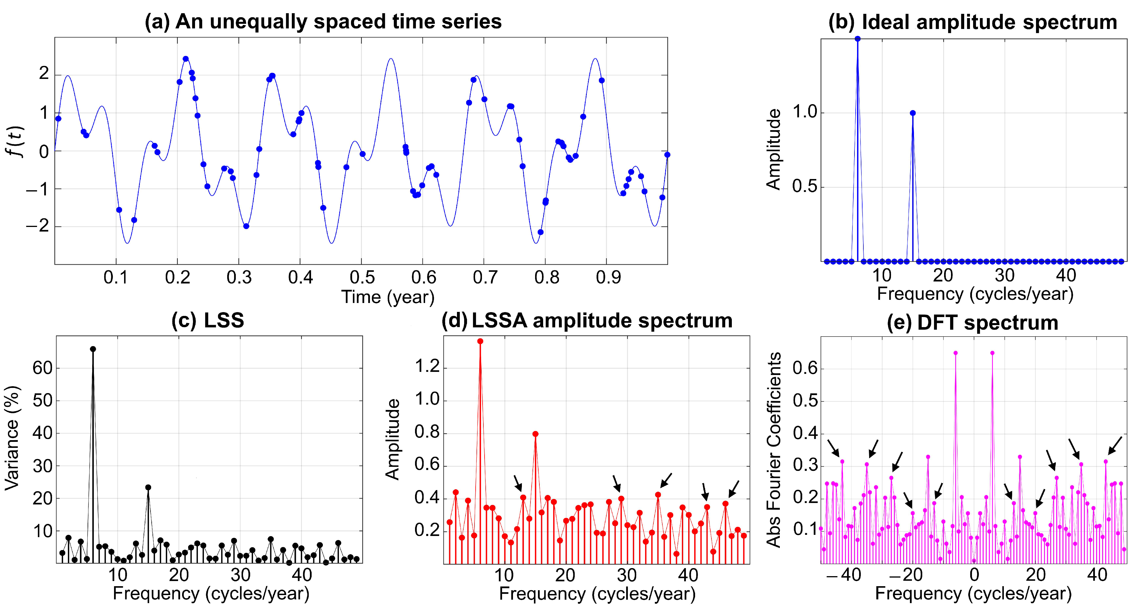
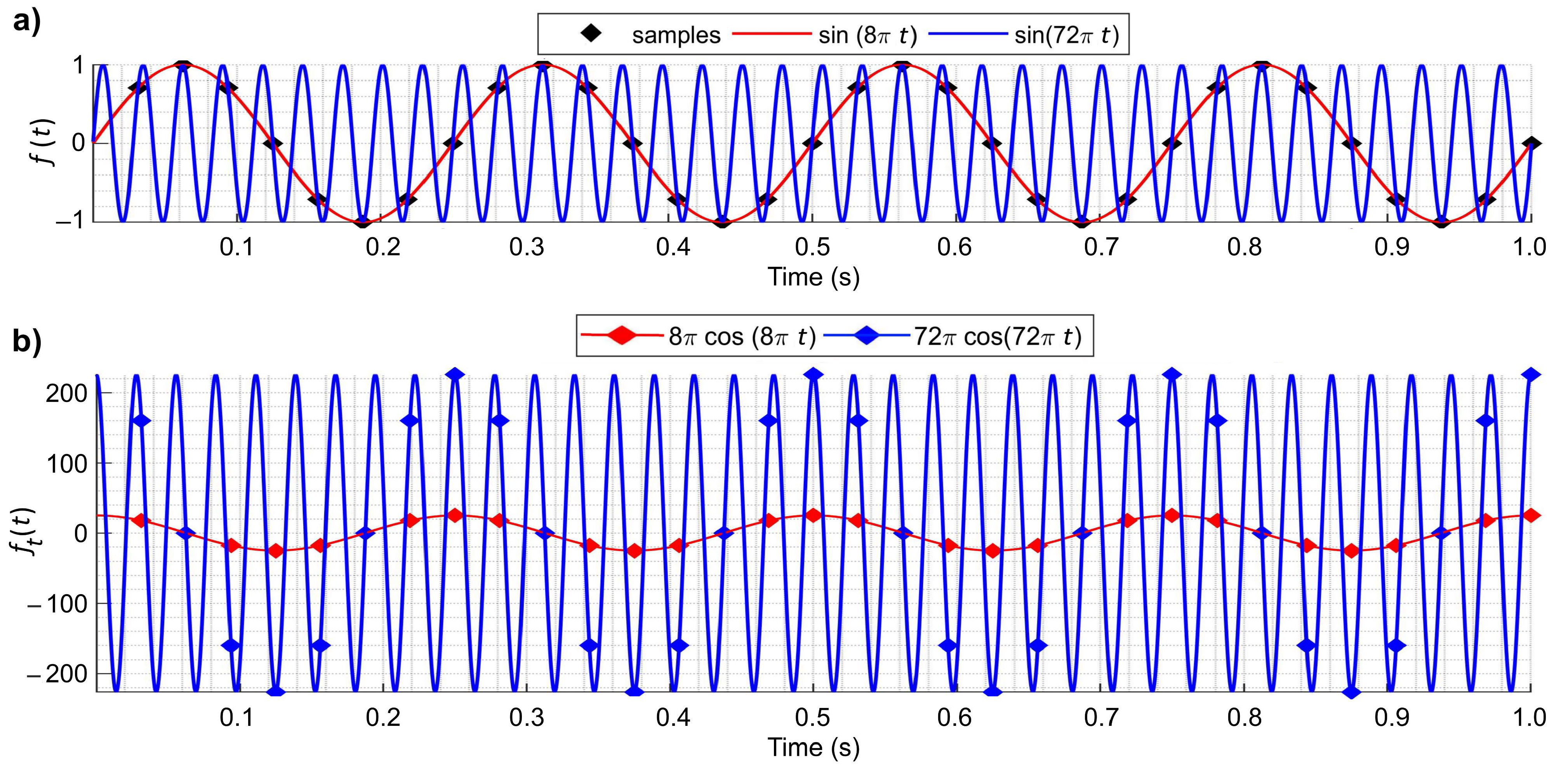
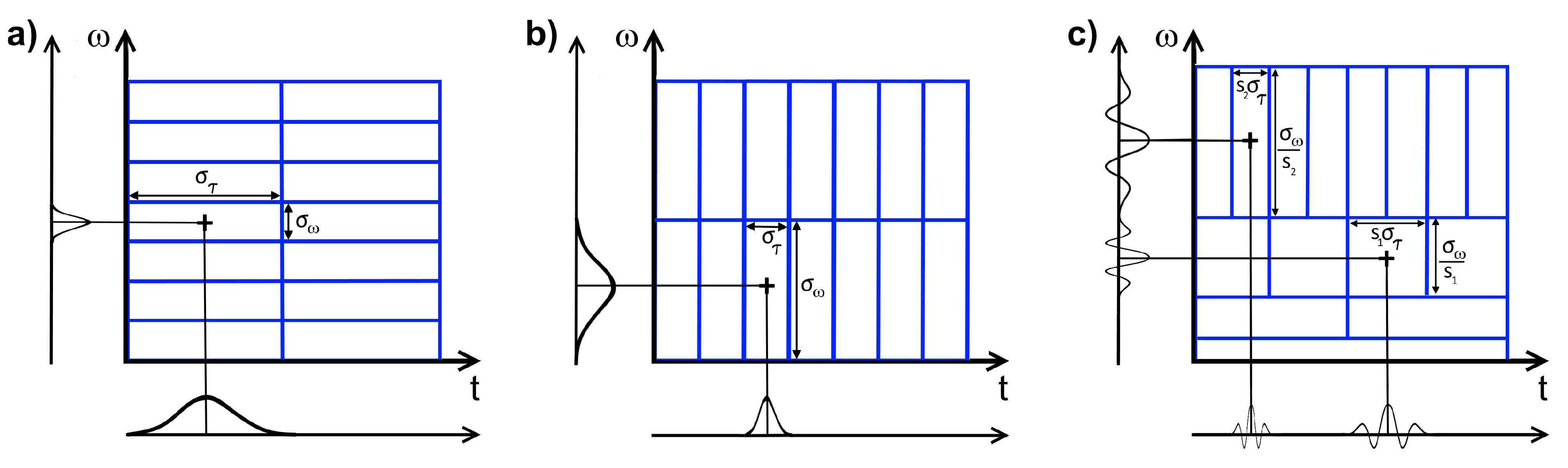
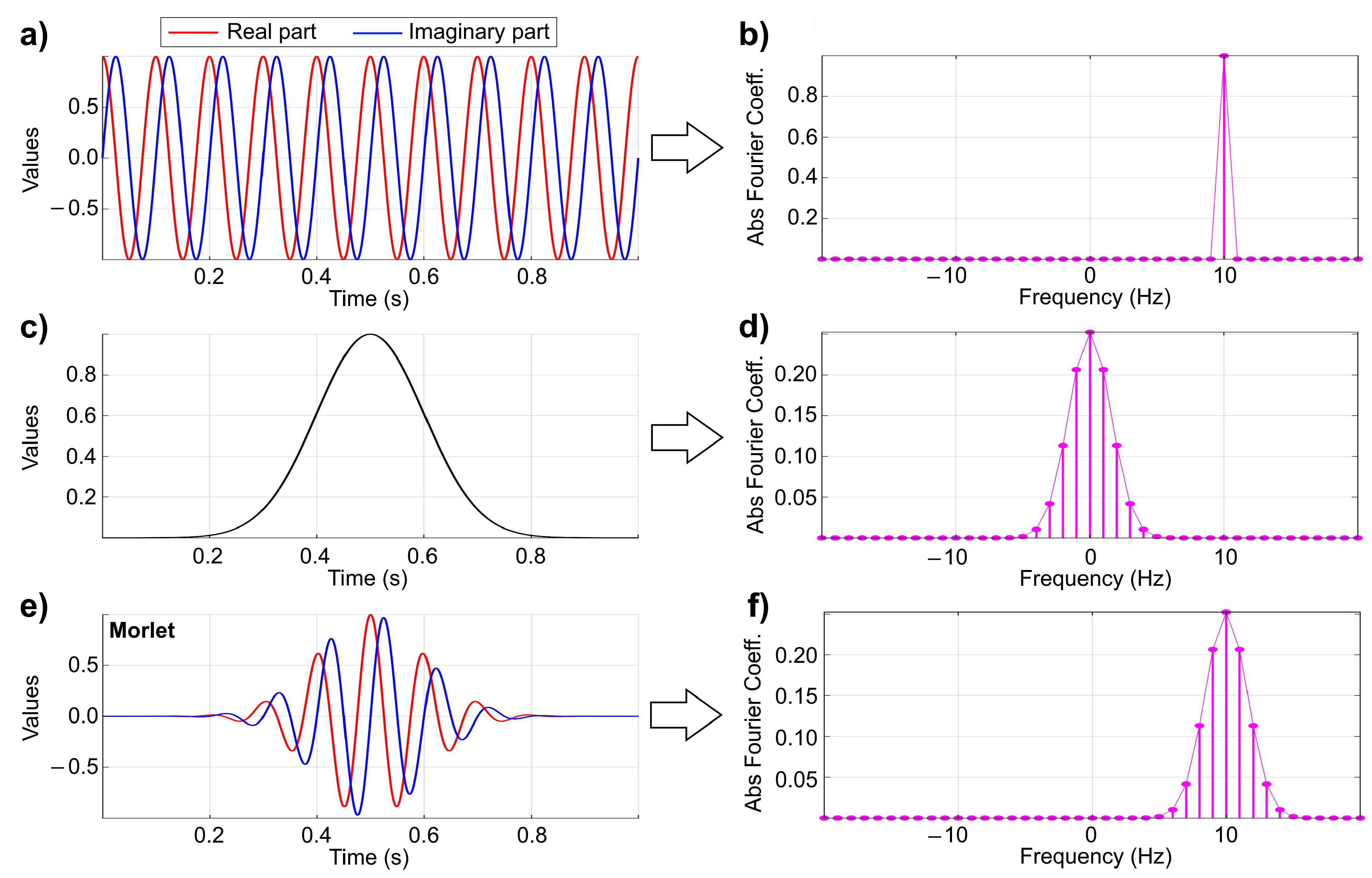
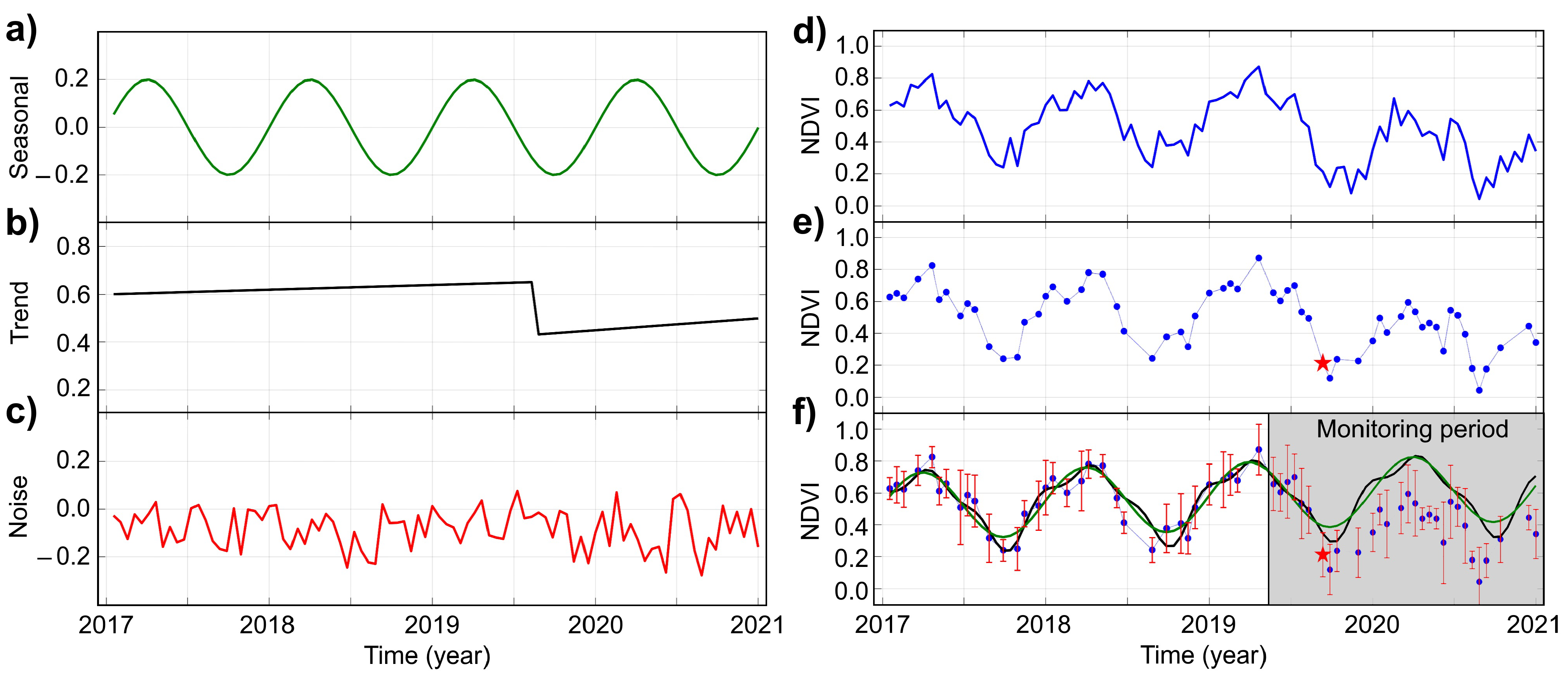
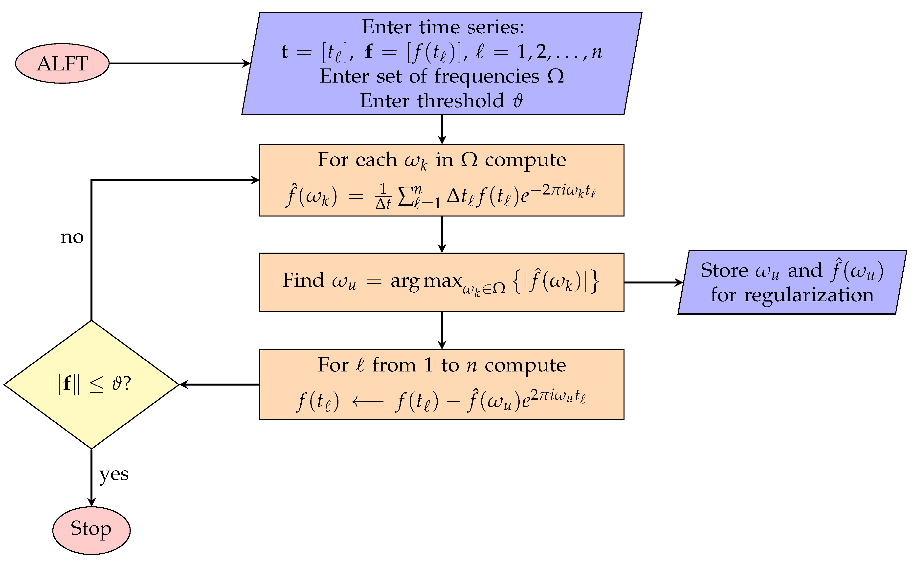
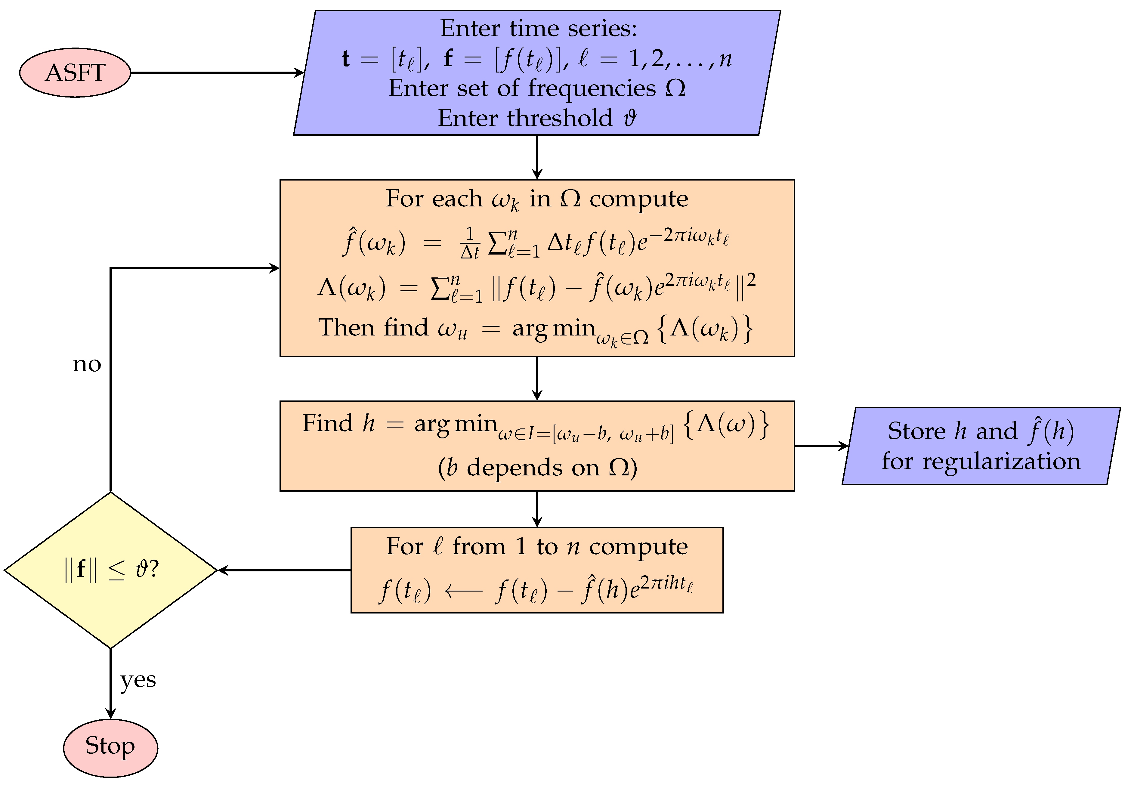
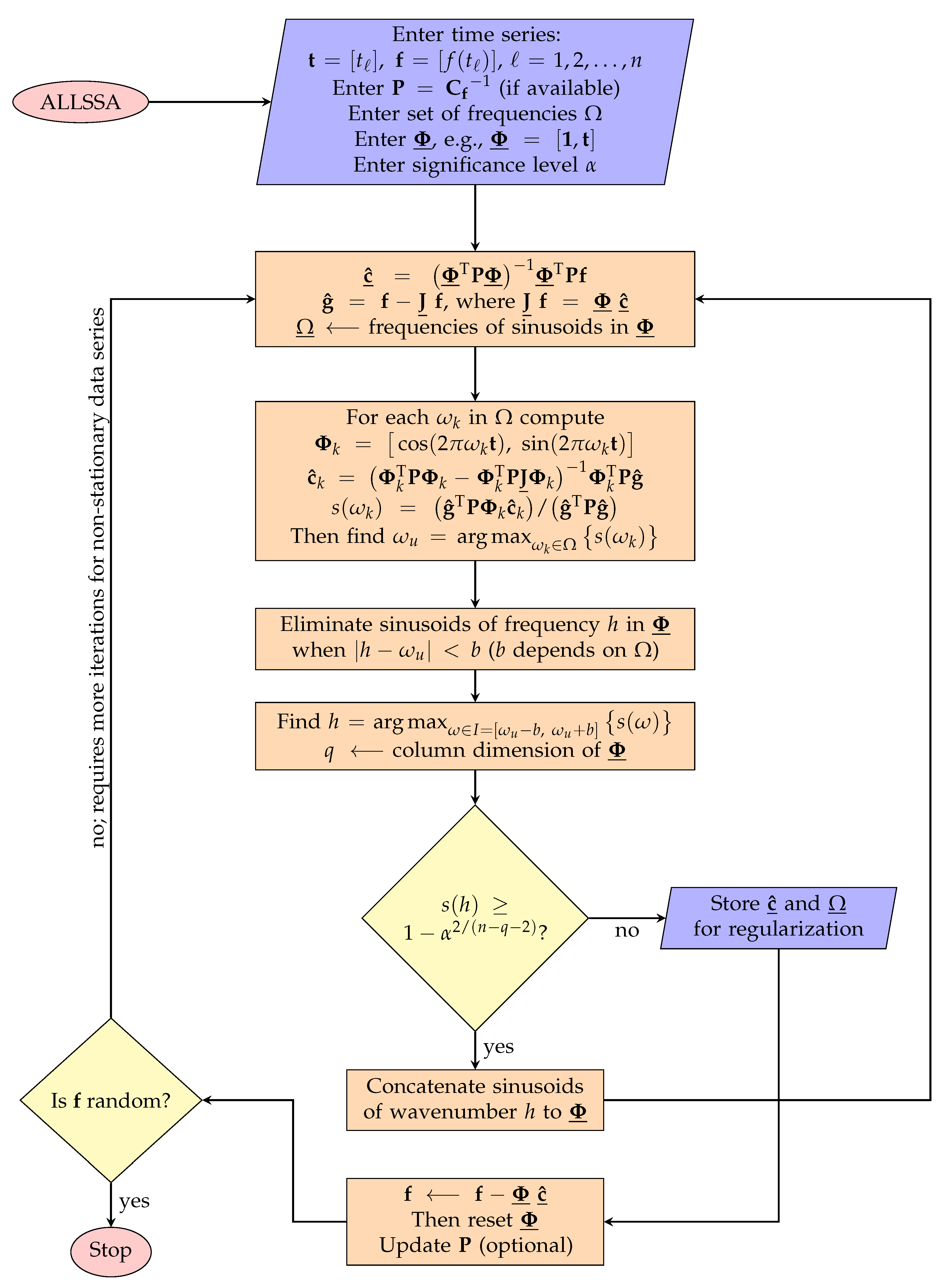
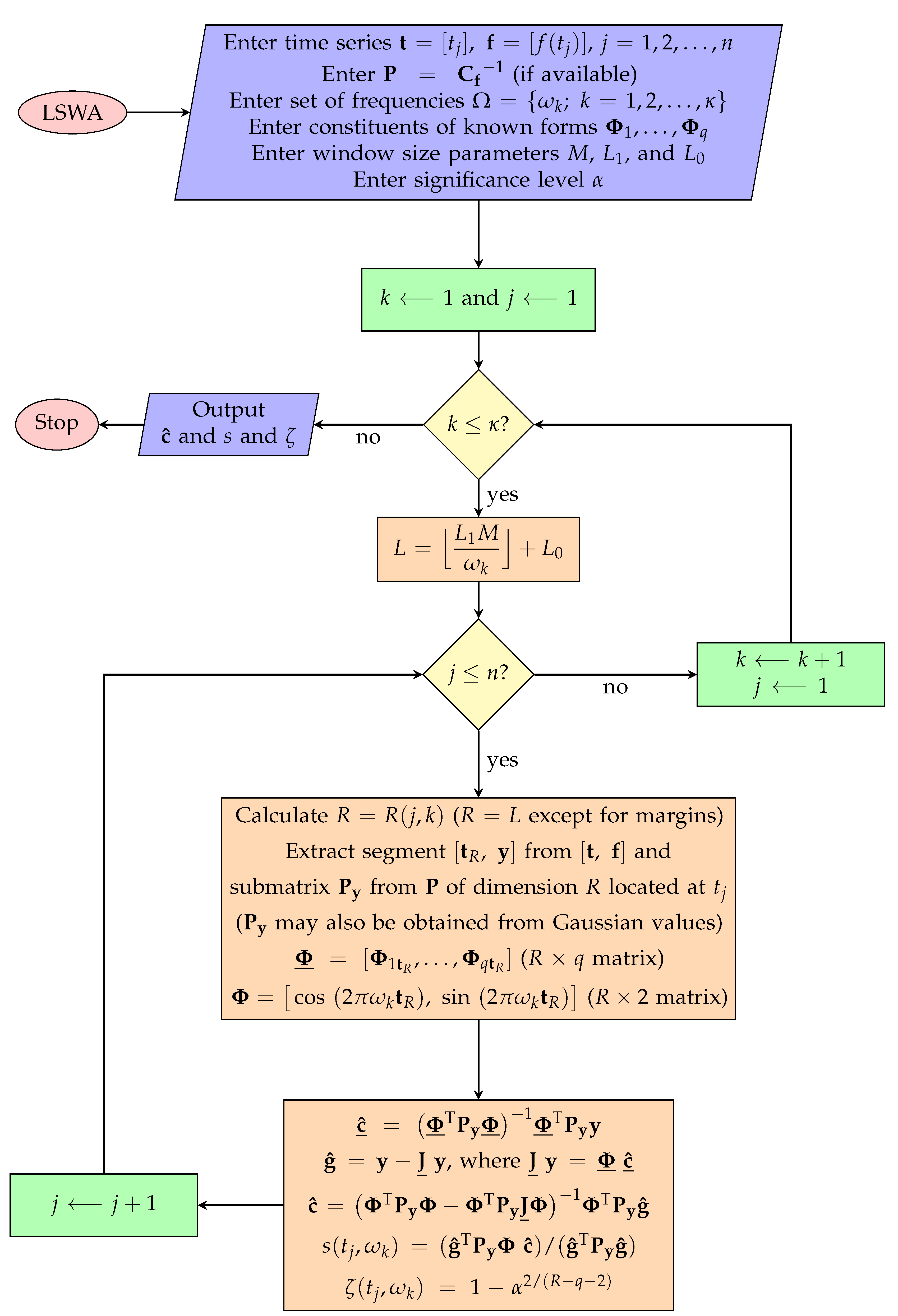
Table 1. Some of the applications of the methods reviewed in this paper.

Field	Data/Time Series	Description	References
Geodesy	Very Long Baseline Interferometry (VLBI) and Temperature Data—GRACE and GOCE Data	LSSA, LSWA, and LSCWA are applied to VLBI and temperature time series; the methods are also applied to study the behavior of GRACE stripes in space-frequency domains	[43,60,94,95]
Geophysics	Marine Seismic and Multicomponent Streamer Data	ALFT, ASFT, IMAP, MIMAP, ALLSSA and MALLSSA are applied to regularize coarsely sampled seismic data	[19,20,21,22,23,24,25,26,27]
Remote Sensing	MODIS and Landsat Imagery	BFAST, BFAST Monitor, CCDC, DBEST, EWMACD, JUST, and JUST Monitor as well as LSWA and LSCWA and other similar methods are applied for vegetation and drought monitoring, forecasting forest fire danger conditions, and crop yield forecasting	[65,66,71,73,76,77,89,90,91,92,96,97,98,99,100]
Astronomy	Telescope Observations—AAVSO	WWA, WWZ, HHT, LSSA, ALLSSA, and LSWA are applied to study the orbital, pulsation, and spin periods of variable stars and others	[42,51,101]
Hydrology	Streamflow and Climate Data	CWT, XWT, HHT, LSWA, LSCWA, and other similar methods are applied to study inter- and intra-annual fluctuations in streamflow and climate time series for flow forecasting and other purposes	[102,103,104,105,106,107]
Finance	Stock exchange and price series; daily Eurozone stock market	CWT, DWT, maximal overlap DWT, and wavelet coherency are applied to analyze financial time series	[108,109,110,111]
Medicine	Electroencephalogram (EEG) and Electrocardiogram (ECG) Signals	CWT, DWT, EMD, and EWT are applied to the EEG and ECG signals to study brain and heart activities	[112,113,114]

MODIS: Moderate Resolution Imaging Spectroradiometer; AAVSO: American Association of Variable Star Observers; GRACE: Gravity Recovery and Climate Experiment; GOCE: Gravity field and steady-state Ocean Circulation Explorer.

lists some of the applications of the change detection and time-frequency analyses mentioned herein.

6. Conclusions

In this paper, many frequency and time-frequency decomposition methods via Fourier and least-squares analyses were studied. Many change detection and monitoring methods were also briefly reviewed, and some of the applications of all methods were listed in Table 1. There are many more robust time series analysis techniques proposed by researchers that were not mentioned here. In many practical applications, time series contain seasonal and trend components. Simultaneous estimation of the statistically significant components can provide more accurate and reliable estimates for the time series components and thus are more appropriate for change detection and monitoring. The time series components can also be estimated more accurately when considering the observational uncertainties. Therefore, the observations with higher uncertainties hold less weight during the analysis and vice versa. Computational complexity optimization is another major challenge in time series analysis when dealing with big data sets. An inappropriate algorithm modification for reducing the computational cost can produce unreliable and inaccurate results. Each method presented herein has advantages and weaknesses, and there is plenty of room for researchers and scientists to expand and improve the existing methods. Finally, we conclude this by the following quote from Nikola Tesla (1856–1943).

If you want to find the secrets of the universe, think in terms of energy, frequency, and vibration. We are just waves in time and space, changing continuously, and the illusion of individuality is produced through the concatenation of the rapidly succeeding phases of existence. What we define as likeness is merely the result of the symmetrical arrangement of molecules that compose our bodies.

References

- Mallat, S. A Wavelet Tour of Signal Processing; Academic Press: Cambridge, UK, 1999. [Google Scholar]
- Brown, R.G.; Hwang, P.Y.C. Introduction to Random Signals and Applied Kalman Filtering; John Wiley and Sons, Inc.: Hoboken, NJ, USA, 2012. [Google Scholar]
- Craymer, M.R. The Least-Squares Spectrum, Its Inverse Transform and Autocorrelation Function: Theory and Some Application in Geodesy. Ph.D. Thesis, University of Toronto, Toronto, ON, Canada, 1998. [Google Scholar]
- Ghaderpour, E. Least-Squares Wavelet Analysis and Its Applications in Geodesy and Geophysics. Ph.D. Thesis, York University, Toronto, ON, Canada, 2018. [Google Scholar]
- Vaníček, P.; Krakiwsky, E.J. Geodesy the Concepts, 2nd ed.; Elsevier: Amsterdam The Netherlands, 1986. [Google Scholar]
- Craig, A.T.; Hogg, R.V.; McKean, J. Introduction to Mathematical Statistics, 7th ed.; Pearson Education: London, UK, 2013. [Google Scholar]
- Fourier, J.B.J. The Analytical Theory of Heat; Translated by Alexander Freeman; The University Press: Cambridge, UK, 1878. [Google Scholar]
- Miller, S.; Childers, D. Probability and Random Processes; Academic Press: Cambridge, MA, USA, 2012. [Google Scholar]
- Ware, A.F. Fast approximate Fourier transforms for irregularly spaced data. SIAM Rev. 1998, 40, 838–856. [Google Scholar] [CrossRef]
- Vaníček, P. Approximate spectral analysis by least-squares fit. Astrophys. Space Sci. 1969, 4, 387–391. [Google Scholar] [CrossRef]
- Vaníček, P. Further development and properties of the spectral analysis by least-squares. Astrophys. Space Sci. 1971, 12, 10–33. [Google Scholar] [CrossRef]
- Lomb, N.R. Least-squares frequency analysis of unequally spaced data. Astrophys. Space Sci. 1976, 39, 447–462. [Google Scholar] [CrossRef]
- Pagiatakis, S. Stochastic significance of peaks in the least-squares spectrum. J. Geod. 1999, 73, 67–78. [Google Scholar] [CrossRef]
- Wells, D.E.; Vaníček, P.; Pagiatakis, S.D. Least-Squares Spectral Analysis Revisited; Department of Surveying Engineering, University of New Brunswick: Fredericton, NB, Canada, 1985. [Google Scholar]
- Wells, D.E.; Krakiwsky, E.J. The Method of Least-Squares; Department of Surveying Engineering, University of New Brunswick: Fredericton, NB, Canada, 1971. [Google Scholar]
- VanderPlas, J.T. Understanding the Lomb–Scargle Periodogram. Astrophys. J. Suppl. Ser. 2018, 236, 28. [Google Scholar] [CrossRef]
- Seberry, J.; Wysocki, B.J.; Wysocki, T.A. On some applications of Hadamard matrices. Metrika 2005, 62, 221–239. [Google Scholar] [CrossRef] [Green Version]
- Ghaderpour, E.; Kharaghani, H. The asymptotic existence of orthogonal designs. Australas. J. Comb. 2014, 58, 333–346. [Google Scholar]
- Ghaderpour, E.; Liao, W.; Lamoureux, M.P. Antileakage least-squares spectral analysis for seismic data regularization and random noise attenuation. Geophysics 2018, 83, V157–V170. [Google Scholar] [CrossRef]
- Xu, S.; Zhang, Y.; Pham, D.; Lambaré, G. Antileakage Fourier transform for seismic data regularization. Geophysics 2005, 70, V87–V95. [Google Scholar] [CrossRef]
- Xu, S.; Zhang, Y.; Lambaré, G. Antileakage Fourier transform for seismic data regularization in higher dimensions. Geophysics 2010, 75, WB113–WB120. [Google Scholar] [CrossRef]
- Guo, Z.; Zheng, Y.; Liao, W. High Fidelity Seismic Trace Interpolation. In SEG Technical Program Expanded Abstracts; Society of Exploration Geophysicists: Tulsa, OK, USA, 2015; pp. 3915–3919. [Google Scholar] [CrossRef] [Green Version]
- Hollander, Y.; Kosloff, D.; Koren, Z.; Bartana, A. Seismic Data Interpolation by Orthogonal Matching Pursuit. In Proceedings of the 74th EAGE Conference and Exhibition Incorporating EUROPEC, Copenhagen, Denmark, 4 June 2012. [Google Scholar] [CrossRef]
- Özbek, A.; Özdemir, A.K.; Vassallo, M. Interpolation by Matching Pursuit. In SEG Technical Program Expanded Abstracts; Society of Exploration Geophysicists: Tulsa, OK, USA, 2009; pp. 3254–3258. [Google Scholar] [CrossRef]
- Vassallo, M.; Özbek, A.; Özdemir, A.K.; Eggenberger, K. Crossline wavefield reconstruction from multicomponent streamer data: Part 1-multichannel interpolation by matching pursuit (MIMAP) using pressure and its crossline gradient. Geophysics 2010, 75, WB53–WB67. [Google Scholar] [CrossRef]
- Vassallo, M.; Özbek, A.; Özdemir, A.K.; WesternGeco; Eggenberger, K. Crossline wavefield reconstruction from multicomponent streamer data: Multichannel interpolation by matching pursuit. In SEG Technical Program Expanded Abstracts; Society of Exploration Geophysicists: Tulsa, OK, USA, 2010; pp. 3594–3598. [Google Scholar] [CrossRef] [Green Version]
- Ghaderpour, E. Multichannel antileakage least-squares spectral analysis for seismic data regularization beyond aliasing. Acta Geophys. 2019, 67, 1349–1363. [Google Scholar] [CrossRef]
- Gabor, D. Theory of communication. J. IEEE 1946, 93, 429–457. [Google Scholar] [CrossRef]
- Weyl, H. The Theory of Groups and Quantum Mechanics; Courier Corporation: Dutton, NY, USA, 1931. [Google Scholar]
- Morlet, J. Sampling theory and wave propagation. In Issues in Acoustic Signal-Image Processing and Recognition; Chen, C.H., Ed.; NATO ASI Series (Series F: Computer and System Sciences); Springer: Berlin, Germany, 1983; Volume 1, pp. 233–261. [Google Scholar]
- Grossmann, A.; Morlet, J.; Paul, T. Transforms associated to square integrable group representations. I General results. J. Math. Phys. 1985, 26, 2473–2479. [Google Scholar] [CrossRef]
- Grossmann, A.; Morlet, J.; Paul, T. Transforms associated to square integrable group representations. II examples. Ann. Inst. Henri Poincare Phys. Theor. 1986, 45, 293–309. [Google Scholar]
- Hlawatsch, F.; Boudreaux-Bartels, F. Linear and quadratic time-frequency signal representations. IEEE Signal Process. Mag. 1992, 9, 21–67. [Google Scholar] [CrossRef]
- Daubechies, I. The wavelet transform, time-frequency localization and signal analysis. IEEE Trans. Inf. Theory 1990, 36, 961–1005. [Google Scholar] [CrossRef] [Green Version]
- Farge, M. Wavelet transforms and their applications to turbulence. Ann. Rev. Fluid Mech. 1992, 24, 395–457. [Google Scholar] [CrossRef]
- Misiti, M.; Misiti, Y.; Oppenheim, G.; Poggi, J.M. Wavelet Toolbox: User’s Guide (MATLAB). Available online: http://ailab.chonbuk.ac.kr/seminar_board/pds1_files/w7_1a.pdf (accessed on 30 June 2021).
- Grinsted, A.; Moore, J.C.; Jeverjeva, S. Application of the cross-wavelet transform and wavelet coherence to geophysical time series. Nonlinear Process. Geophys. 2004, 11, 561–566. [Google Scholar] [CrossRef]
- Torrence, C.; Compo, G.P. A practical guide to wavelet analysis. Bull. Am. Meteorol. Soc. 1998, 79, 61–78. [Google Scholar] [CrossRef] [Green Version]
- Rhif, M.; Ben Abbes, A.; Farah, I.R.; Martinez, B.; Sang, Y. Wavelet transform application for/in non-stationary time-series analysis: A review. Appl. Sci. 2019, 9, 1345. [Google Scholar] [CrossRef] [Green Version]
- Hall, P.; Turlach, B.A. Interpolation methods for nonlinear wavelet regression with irregularly spaced design. Ann. Stat. 1997, 25, 1912–1925. [Google Scholar] [CrossRef]
- Sardy, S.; Percival, D.B.; Bruce, A.G.; Gao, H.; Stuetzle, W. Wavelet shrinkage for unequally spaced data. Stat. Comput. 1999, 9, 65–75. [Google Scholar] [CrossRef]
- Foster, G. Wavelet for period analysis of unevenly sampled time series. Astron. J. 1996, 112, 1709–1729. [Google Scholar] [CrossRef]
- Ghaderpour, E.; Pagiatakis, S.D. Least-squares wavelet analysis of unequally spaced and non-stationary time series and its applications. Math. Geosci. 2017, 49, 819–844. [Google Scholar] [CrossRef]
- Qian, S. Introduction to Time-Frequency and Wavelet Transforms; Prentice-Hall Inc.: Upper Saddle River, NJ, USA, 2002. [Google Scholar]
- Wijaya, D.R.; Sarno, R.; Zulaika, E. Information Quality Ratio as a novel metric for mother wavelet selection. Chemom. Intell. Lab. Syst. 2017, 160, 59–71. [Google Scholar] [CrossRef]
- Van Valkenburg, M.E. Network Analysis, 3rd ed.; Pearson Education: London, UK, 2006. [Google Scholar]
- A Practical Guide to Wavelet Analysis–by Torrence and Compo. Software for Fortran, IDL, Matlab, and Python. Available online: https://atoc.colorado.edu/research/wavelets/ (accessed on 30 June 2021).
- Huang, N.E.; Shen, Z.; Long, S.R.; Wu, M.C.; Shih, H.H.; Zheng, Q.; Yen, N.C.; Tung, C.C.; Liu, H.H. The empirical mode decomposition and the Hilbert spectrum for nonlinear and non-stationary time series analysis. Proc. R. Soc. Lond. A 1998, 454, 903–995. [Google Scholar] [CrossRef]
- Huang, N.E.; Wu, Z. A review on Hilbert-Huang transform: Method and its applications to geophysical studies. Rev. Geophys. 2008, 46, 1–23. [Google Scholar] [CrossRef] [Green Version]
- Huang, N.E.; Wu, Z. Ensemble empirical mode decomposition: A noise-assisted data analysis method. Adv. Adapt Data Anal. 2009, 1, 1–41. [Google Scholar]
- Barnhart, B.L. The Hilbert-Huang Transform: Theory, Application, Development. Ph.D. Thesis, University of Iowa, Iowa, IA, USA, 2011. [Google Scholar]
- Chen, Y.; Feng, M.Q. A technique to improve the empirical mode decomposition in the Hilbert-Huang transform. Earthq. Eng. Eng. Vib. 2003, 2, 75–85. [Google Scholar] [CrossRef] [Green Version]
- Guang, Y.; Sun, X.; Zhang, M.; Li, X.; Liu, X. Study on ways to restrain end effect of Hilbert-Huang transform. J. Comput. 2014, 25, 22–31. [Google Scholar]
- Datig, M.; Schlurmann, T. Performance and limitations of the Hilbert-Huang transformation (HHT) with an application to irregular water waves. Ocean Eng. 2004, 31, 1783–1834. [Google Scholar] [CrossRef]
- Puryear, C.I.; Portniaguine, O.N.; Cobos, C.M.; Castagna, J.P. Constrained least-squares spectral analysis: Application to seismic data. Geophysics 2012, 77, 143–167. [Google Scholar] [CrossRef]
- Rao, C.R.; Mitra, S.K. Generalized Inverse of Matrices and Its Applications; John Wiley: New York, NY, USA, 1971. [Google Scholar]
- Puryear, C.I. Constrained Least-Squares Spectral Analysis: Application to Seismic Data. Ph.D. Thesis, University of Houston, Houston, TX, USA, 2012. [Google Scholar]
- Abramowitz, M.; Stegun, I.A. Handbook of Mathematical Functions with Formulas, Graphs, and Mathematical Tables; National Bureau of Standards Applied Mathematics Series; USA Department of Commerce: Washington, DC, USA, 1972. [Google Scholar]
- Ge, Z. Significance tests for the wavelet cross-spectrum and wavelet linear coherence. Ann. Geophys. 2008, 26, 3819–3829. [Google Scholar] [CrossRef]
- Ghaderpour, E.; Ince, E.S.; Pagiatakis, S.D. Least-squares cross-wavelet analysis and its applications in geophysical time series. J. Geod. 2018, 92, 1223–1236. [Google Scholar] [CrossRef]
- Ghaderpour, E.; Pagiatakis, S.D. LSWAVE: A MATLAB software for the least-squares wavelet and cross-wavelet analyses. GPS Solut. 2019, 23, 50. [Google Scholar] [CrossRef]
- LSWAVE: AMATLAB Software for the Least-SquaresWavelet and Cross-Wavelet Analyses–by E. Ghaderpour and S. D. Pagiatakis. National Geodetic Survey (NGS)—National Oceanic and Atmospheric Administration (NOAA). Available online: https://geodesy.noaa.gov/gps-toolbox/LSWAVE.htm (accessed on 30 June 2021).
- Signal Processing by E. Ghaderpour. GitHub. Available online: https://github.com/Ghaderpour/LSWAVE-SignalProcessing/ (accessed on 30 June 2021).
- Liu, H.Q.; Huete, A. A feedback based modification of the NDVI to minimize canopy background and atmospheric noise. IEEE Trans. Geosci. Remote Sens. 1995, 33, 457–465. [Google Scholar] [CrossRef]
- Verbesselt, J.; Hyndman, R.; Newnham, G.; Culvenor, D. Detecting trend and seasonal changes in satellite image time series. Remote Sens. Environ. 2010, 114, 106–115. [Google Scholar] [CrossRef]
- Verbesselt, J.; Hyndman, R.; Zeileis, A.; Culvenor, D. Phenological change detection while accounting for abrupt and gradual trends in satellite image time series. Remote Sens. Environ. 2010, 114, 2970–2980. [Google Scholar] [CrossRef] [Green Version]
- Breaks for Additive Seasonal and Trend (BFAST) R-Code. Available online: https://cran.r-project.org/web/packages/bfast/index.html (accessed on 30 June 2021).
- Saxena, R.; Watson, L.T.; Wynne, R.H.; Brooks, E.B.; Thomas, V.A.; Zhiqiang, Y.; Kennedy, R.E. Towards apolyalgorithm for land use change detection. ISPRS J. Photogramm. Remote. Sens. 2018, 144, 217–234. [Google Scholar] [CrossRef]
- Awty-Carroll, K.; Bunting, P.; Hardy, A.; Bell, G. An evaluation and comparison of four dense time series change detection methods using simulated data. Remote Sens. 2019, 11, 2779. [Google Scholar] [CrossRef] [Green Version]
- Watts, L.M.; Laffan, S.W. Effectiveness of the BFAST algorithm for detecting vegetation response patterns in a semi-arid region. Remote Sens. Environ. 2014, 154, 234–245. [Google Scholar] [CrossRef]
- Verbesselt, J.; Zeileis, A.; Herold, M. Near real-time disturbance detection using satellite image time series. Remote Sens. Environ. 2012, 123, 98–108. [Google Scholar] [CrossRef]
- Hamunyela, E.; Rosca, S.; Mirt, A.; Engle, E.; Herold, M.; Gieseke, F.; Verbesselt, J. Implementation of BFASTmonitor algorithm on Google Earth Engine to support large-area and sub-annual change monitoring using Earth Observation Data. Remote Sens. 2020, 12, 2953. [Google Scholar] [CrossRef]
- Zhu, Z.; Woodcock, C.E. Continuous change detection and classification of land cover using all available Landsat data. Remote Sens. Environ. 2014, 144, 152–171. [Google Scholar] [CrossRef] [Green Version]
- Zhu, Z.; Woodcock, C.E.; Holden, C.; Yang, Z. Generating synthetic Landsat images based on all available Landsat data: Predicting Landsat surface reflectance at any given time. Remote Sens. Environ. 2015, 162, 67–83. [Google Scholar] [CrossRef]
- Bento, J. On the complexity of the weighted fused lasso. IEEE Signal Process. Lett. 2018, 25, 1595–1599. [Google Scholar] [CrossRef] [Green Version]
- Ghaderpour, E.; Vujadinovic, T. Change detection within remotely-sensed satellite image time series via spectral analysis. Remote Sens. 2020, 12, 4001. [Google Scholar] [CrossRef]
- Ghaderpour, E.; Vujadinovic, T. The potential of the least-squares spectral and cross-wavelet analyses for near-real-time disturbance detection within unequally spaced satellite image time series. Remote Sens. 2020, 12, 2446. [Google Scholar] [CrossRef]
- Ghaderpour, E. JUST: MATLAB and Python software for change detection and time series analysis. GPS Solut. 2021, 25, 85. [Google Scholar] [CrossRef]
- Classen, T.A.C.M.; Mecklenbrauker, W.F.G. The Wigner distribution: A tool for time-frequency analysis (Parts I, II, III). Philips J. Res. 1980, 35, 217–249. [Google Scholar]
- Waldo, D.; Chitrapu, P.R. On the Wigner-Ville distribution of finite duration signals. Signal Process. 1991, 24, 231–237. [Google Scholar] [CrossRef]
- Baydar, N.; Ball, A. A comparative study of acoustic and vibration signals in detection of gear failures using Wigner-Ville distribution. Mech. Syst. Signal Process. 2001, 15, 1091–1107. [Google Scholar] [CrossRef]
- Gilles, J. Empirical wavelet transform. IEEE Trans. Signal Process. 2013, 61, 3999–4010. [Google Scholar] [CrossRef]
- Selesnick, I.V. Wavelet transform with tunable Q-factor. IEEE Trans. Signal Process. 2011, 59, 3560–3575. [Google Scholar] [CrossRef]
- Ren, H.; Wang, Y.L.; Huang, M.Y.; Chang, Y.L.; Kao, H.M. Ensemble empirical mode decomposition parameters optimization for spectral distance measurement in hyperspectral remote sensing data. Remote Sens. 2014, 6, 2069–2083. [Google Scholar] [CrossRef] [Green Version]
- Amato, U.; Antoniadis, A.; Pensky, M. Wavelet kernel penalized estimation for non-equispaced design regression. Stat. Comput. 2006, 16, 37–55. [Google Scholar] [CrossRef]
- Mathias, A.; Grond, F.; Guardans, R.; Seese, D.; Canela, M.; Diebner, H.H. Algorithms for spectral analysis of irregularly sampled time series. J. Stat. Softw. 2004, 11, 1–27. [Google Scholar] [CrossRef]
- Pagiatakis, S.D.; Yin, H.; Abd El-Gelil, M. Least-squares self-coherency analysis of superconducting gravimeter records in search for the Slichter triplet. Phys. Earth Planet. Inter. 2007, 160, 108–123. [Google Scholar] [CrossRef]
- Abd El-Gelil, M.; Pagiatakis, S.D. Least-squares self-coherence for sub-ngal signal detection in the superconducting gravimeter records. J. Geodyn. 2009, 48, 310–315. [Google Scholar] [CrossRef]
- Jamali, S.; Jönsson, P.; Eklundh, L.; Ardö, J.; Seaquist, J. Detecting changes in vegetation trends using time series segmentation. Remote Sens. Environ. 2015, 156, 182–195. [Google Scholar] [CrossRef]
- Brooks, E.B.; Wynne, R.H.; Thomas, V.A.; Blinn, C.E.; Coulston, J.W. On-the-fly massively multitemporal change detection using statistical quality control charts and landsat data. IEEE Trans. Geosci. Remote Sens. 2014, 52, 3316–3332. [Google Scholar] [CrossRef]
- Brooks, E.B.; Yang, Z.; Thomas, V.A.; Wynne, R.H. Edyn: Dynamic signaling of changes to forests using exponentially weighted moving average charts. Forests 2017, 8, 304. [Google Scholar] [CrossRef] [Green Version]
- Zhu, Z. Change detection using Landsat time series: A review of frequencies, preprocessing, algorithms, and applications. ISPRS J. Photogramm. Remote Sens. 2017, 130, 370–384. [Google Scholar] [CrossRef]
- Aminikhanghahi, S.; Cook, D.J. A survey of methods for time series change point detection. Knowl. Inf. Syst. 2017, 51, 339–367. [Google Scholar] [CrossRef] [Green Version]
- Ghaderpour, E. Least-squares wavelet and cross-wavelet analyses of VLBI baseline length and temperature time series: Fortaleza-Hartrao-Westford-Wettzell. Publ. Astron. Soc. Pac. 2020, 133, 1019. [Google Scholar]
- Peidou, A.; Pagiatakis, S. Stripe mystery in GRACE geopotential models revealed. Geophy. Res. Lett. 2020, 47, 9. [Google Scholar]
- Ahmed, M.R.; Hassan, Q.K.; Abdollahi, M.; Gupta, A. Processing of near real time land surface temperature and its application in forecasting forest fire danger conditions. Sensors 2020, 20, 984. [Google Scholar] [CrossRef] [Green Version]
- Ahmed, M.R.; Hassan, Q.K.; Abdollahi, M.; Gupta, A. Introducing a new remote sensing-based model for forecasting forest fire danger conditions at a four-day scale. Remote Sens. 2019, 11, 2101. [Google Scholar] [CrossRef] [Green Version]
- Ghaderpour, E.; Ben Abbes, A.; Rhif, M.; Pagiatakis, S.D.; Farah, I.R. Non-stationary and unequally spaced NDVI time series analyses by the LSWAVE software. Int. J. Remote Sens. 2019, 41, 2374–2390. [Google Scholar] [CrossRef]
- Mosleh, M.K.; Hassan, Q.K.; Chowdhury, E.H. Development of a remote sensing-based rice yield forecasting model. Span. J. Agric. Res. 2016, 14, e0907. [Google Scholar]
- Hazaymeh, K.; Hassan, Q.K. Remote sensing of agricultural drought monitoring: A state of art review. AIMS Environ. Sci. 2016, 3, 604–630. [Google Scholar] [CrossRef]
- Ghaderpour, E.; Ghaderpour, S. Least-squares spectral and wavelet analyses of V455 Andromedae time series: The life after the super-outburst. Publ. Astron. Soc. Pac. 2020, 132, 1017. [Google Scholar] [CrossRef]
- Labat, D. Wavelet analysis of the annual discharge records of the world’s largest rivers. Adv. Water Resour. 2008, 31, 109–117. [Google Scholar] [CrossRef]
- Rudi, J.; Pabel, R.; Jager, G.; Koch, R.; Kunoth, A.; Bogena, H. Multiscale analysis of hydrologic time series data using the Hilbert-Huang transform. Vadose Zone J. 2010, 9, 925–942. [Google Scholar] [CrossRef]
- Fang, Z.; Bogena, H.R.; Kollet, S.; Koch, J.; Vereecken, H. Spatio-temporal validation of long-term 3D hydrological simulations of a forested catchment using empirical orthogonal functions and wavelet coherence analysis. J. Hydrol. 2015, 529, 1754–1767. [Google Scholar] [CrossRef]
- Schultea, J.A.; Najjar, R.G.; Li, M. The influence of climate modes on streamflow in the Mid-Atlantic region of the United States. J. Hydrol. Reg. Stud. 2016, 5, 80–99. [Google Scholar] [CrossRef] [Green Version]
- Ghaderpour, E.; Vujadinovic, T.; Hassan, Q.A. Application of the Least-Squares Wavelet software in hydrology: Athabasca River Basin. J. Hydrol. Reg. Stud. 2021, 36C, 100847. [Google Scholar] [CrossRef]
- Veiga, V.B.; Hassan, Q.K.; He, J. Development of flow forecasting models in the Bow River at Calgary, Alberta, Canada. Water 2015, 7, 99–115. [Google Scholar] [CrossRef] [Green Version]
- Gallegati, M. Wavelet analysis of stock returns and aggregate economic activity. Comput. Stat. Data Anal. 2008, 52, 3061–3074. [Google Scholar] [CrossRef]
- Fernández-Macho, J. Wavelet multiple correlation and cross-correlation: A multiscale analysis of Eurozone stock markets. Phys. A Stat. Mech. Appl. 2012, 391, 1097–1104. [Google Scholar] [CrossRef] [Green Version]
- Masset, P. Analysis of financial time series using wavelet methods. In Handbook of Financial Econometrics and Statistics; Springer: Berlin, Germany, 2015; pp. 539–573. [Google Scholar]
- Chakrabarty, A.; De, A.; Gunasekaran, A.; Dubey, R. Investment horizon heterogeneity and wavelet: Overview and further research directions. Phys. A Stat. Mech. Appl. 2015, 429, 45–61. [Google Scholar] [CrossRef]
- Addison, P.S. Wavelet transforms and the ECG: A review. Physiol. Meas. 2005, 26, 155–199. [Google Scholar] [CrossRef] [PubMed] [Green Version]
- Bhattacharyya, A.; Sharma, M.; Pachori, R.B.; Sircar, P.; Acharya, U.R. A novel approach for automated detection of focal EEG signals using empirical wavelet transform. Neural Comput. Appl. 2018, 29, 47–57. [Google Scholar] [CrossRef]
- Alickovic, E.; Kevric, J.; Subasi, A. Performance evaluation of empirical mode decomposition, discrete wavelet transform, and wavelet packed decomposition for automated epileptic seizure detection and prediction. Biomed. Signal Process. Control 2018, 39, 94–102. [Google Scholar] [CrossRef]
Figure 1.
Spectral leakages in DFT and LSSA for unequally spaced time series. Arrows show many of the leakages.
Figure 2.
(a) Two aliased sinusoids with identical values at sampling frequency 32 Hz, and (b) their gradients with many different values at sample positions.
Figure 3.
A few adjacent Heisenberg boxes of the STFT (a,b), and CWT (c).
Figure 4.
Morlet wavelet of frequency 10 Hz and its analyses (1000 samples per second). (a) Sinusoids of frequency 10 Hz, (b) DFT spectrum of panel a, (c) a Gaussian function, (d) DFT spectrum of panel c, (e) a Morlet wavelet, and (f) DFT spectrum of panel e.
Figure 5.
Simulation of a 16-day NDVI time series: (a) seasonal component, (b) trend component with an abrupt change in 2019 with a negative magnitude, (c) noise component, (d) the sum of seasonal, trend, and noise components, (e) of the observations are randomly removed, and (f) illustration of near-real-time monitoring. The breakpoint or jump is shown by a red star. The red vertical bars are the error bars. The black curve is the result of an over-fitting issue that arises when the sinusoids of frequencies 1,2,3 cycles per year are forced to be fitted to the stable time series segment, so when the result is forecast into the monitoring period, shown in the gray background, the breakpoint may not be correctly detected.