
Comparative Analysis of Low Discrepancy Sequence-Based Initialization Approaches Using Population-Based Algorithms for Solving the Global Optimization Problems

 , , ,
, , ,  and
and
Abstract
:1. Introduction
2. Related Work
3. Methodology
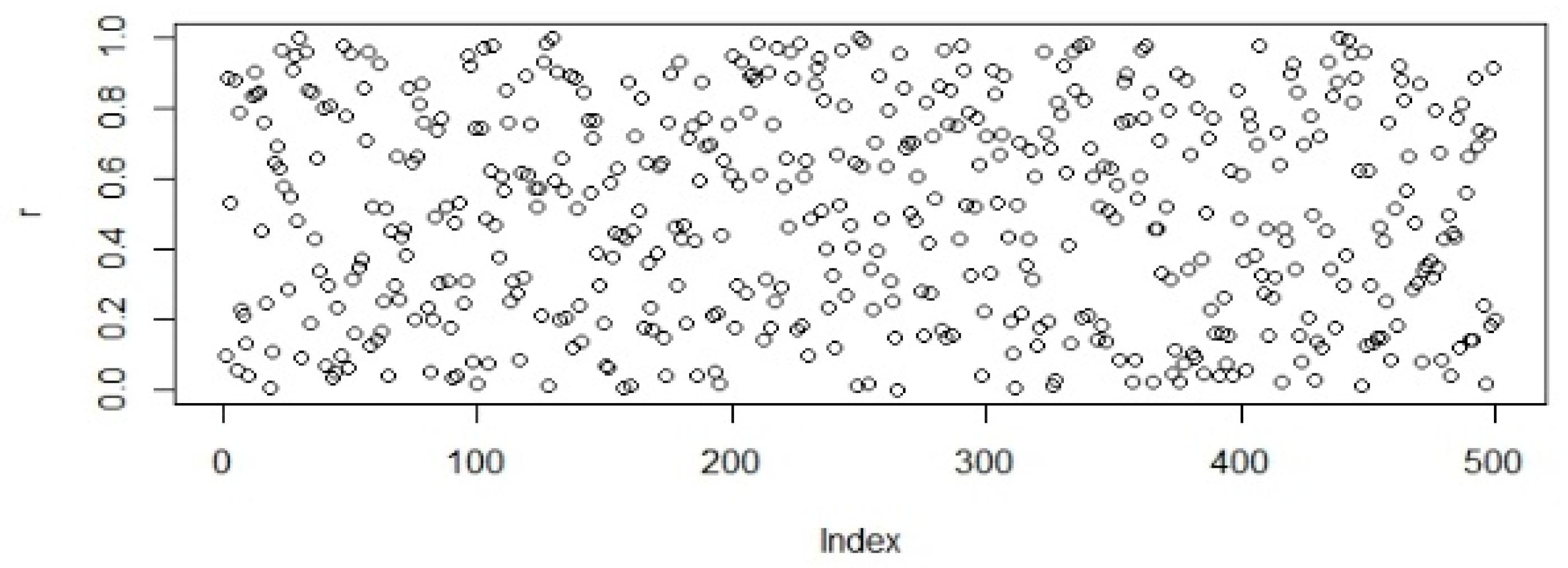
3.1. Random Number Generator
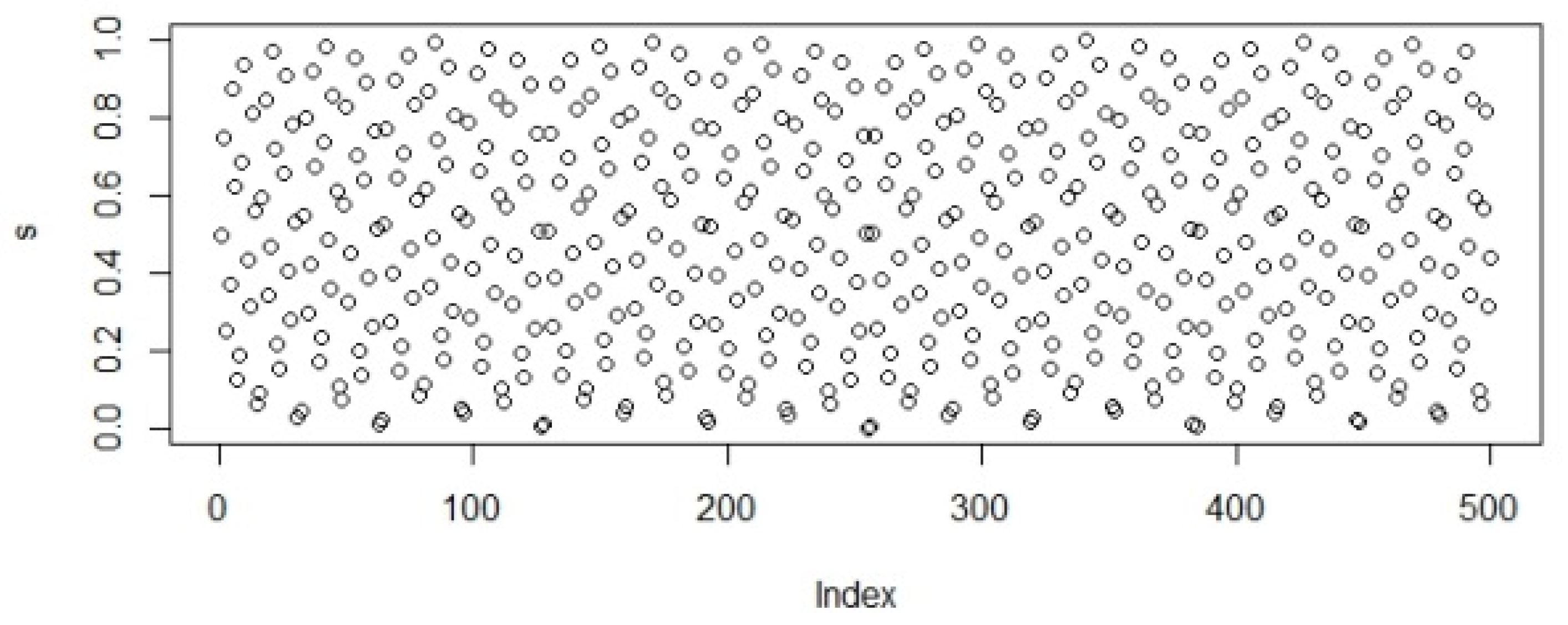
3.2. The Sobol Sequence
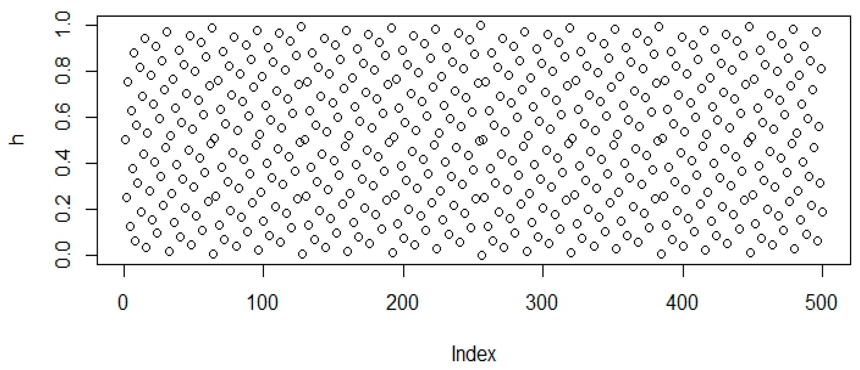
3.3. The Halton Sequence
| Algorithm 1 Halton Sequences |
| Halton (): // input: Size = and base = with Dimension = // output: population instances = Fix the interval over For each iteration : do For each particle |
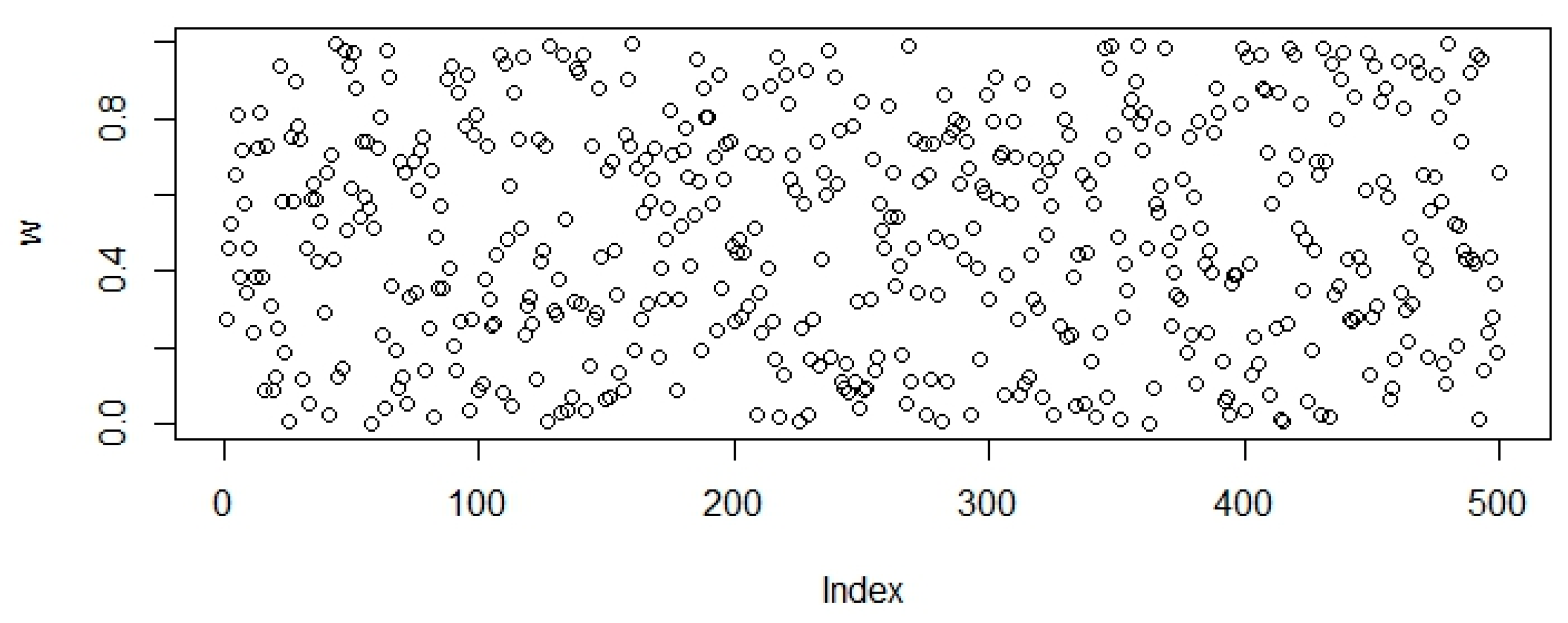
3.4. The Well Sequence
| Algorithm 2 WELL Sequences |
| WELL (): for Return |
3.5. The Knuth Sequence
3.6. The Torus Sequence
| Algorithm 3 Proposed Pseudocode of PSO Using Novel Method of Initialization |
|
| Algorithm 4 Proposed Pseudo Code of DE Using Novel Method of Initialization |
| Input: 𝑥𝑖 = (𝑥𝑖,1, 𝑥𝑖,2, 𝑥𝑖,3, …, 𝑥𝑖,𝐷), Population size ‘N-P’, Problem Size ‘D’, Mutation Rate ‘F’, Crossover Rate ‘C-R’; Stopping Criteria {Number of Generation, Target}, Upper Bound ‘U’, Lower Bound ‘L’ Output: 𝑥𝑖, = Global fitness vector with minimal fitness value Pop = Initialize of Paraments (N-P, D, U, L); Generate initial population Using WELL,Knuth,Torus While (Stopping Criteria ≠ True) do Best Vector = Evaluate Pop (Pop); vx = Select Rand Vector (Pop); I = Find Index Vector (vx); Select Rand Vector (Pop,v1,v2,v3) where v1 ≠ v2 ≠ v3 ≠ vx vy = v1, + F(v2−v3) For (i = 0; i++; i < D−1) If (randj [0, 1) < C-R) Then U[i] = vx [i]. else U[i] = vy [i] End For loop If (Cost Fun Vector(U) ≤ Cost Fun Vector (vx)) Then Update Pop (U, I, Pop); End IF End While Retune Best Vector |
4. Experimental Setup
5. Simulation Results and Discussion
5.1. Results and Graphs on PSO Approaches
5.2. Friedman and Kruskal–Wallis Test on PSO Approaches
5.3. Discussion on PSO Results
A. Discussion
- Effect of using different initializing PSO approaches
- Effect of using different dimensions for problems
- A comparative analysis
- i.
- Effect of Using Different Initializing PSO Approaches
- ii.
- Effect of Using Different Dimensions for Problems
- iii.
- Comparative Analysis
5.4. Discussion on DE Results
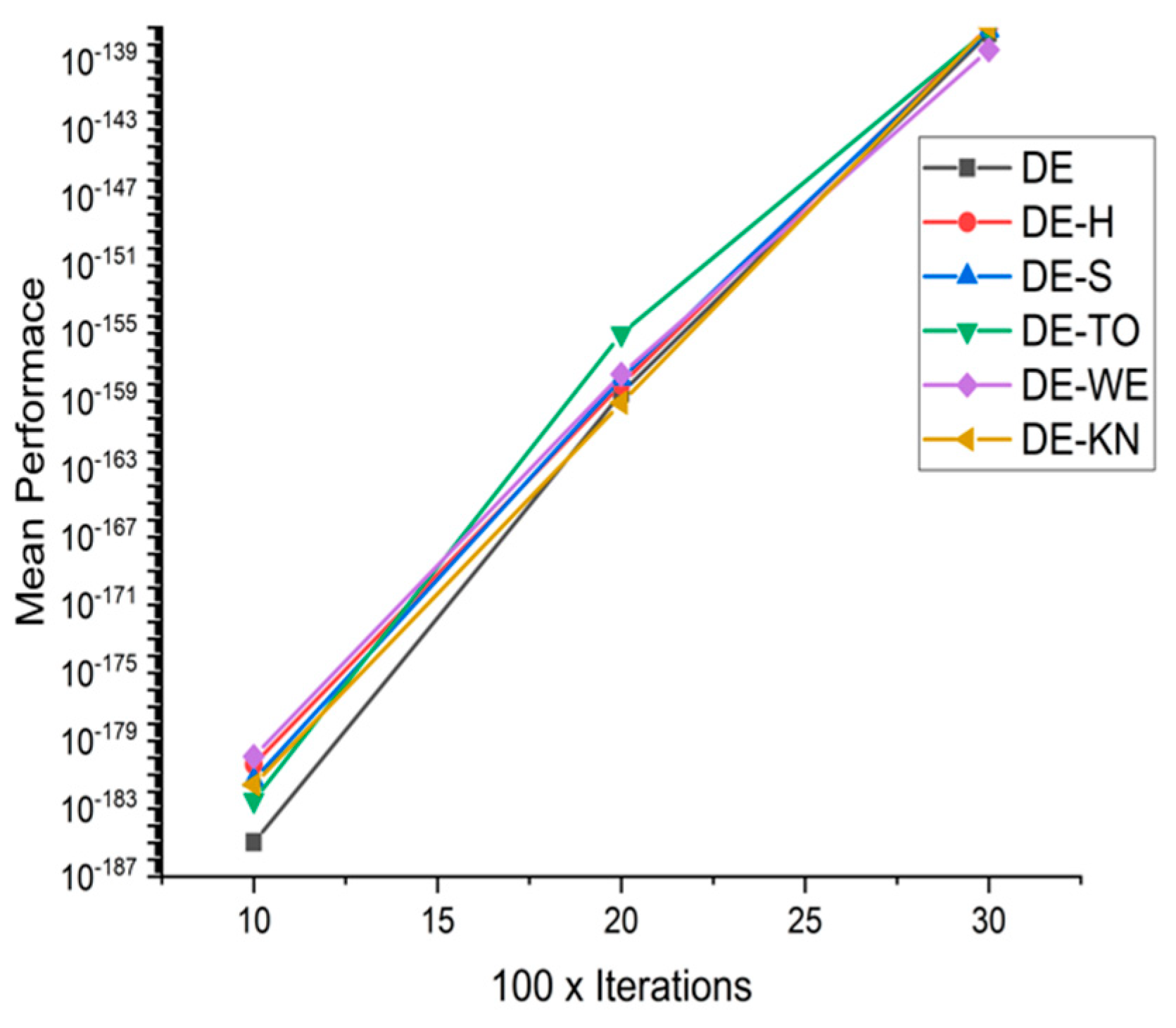
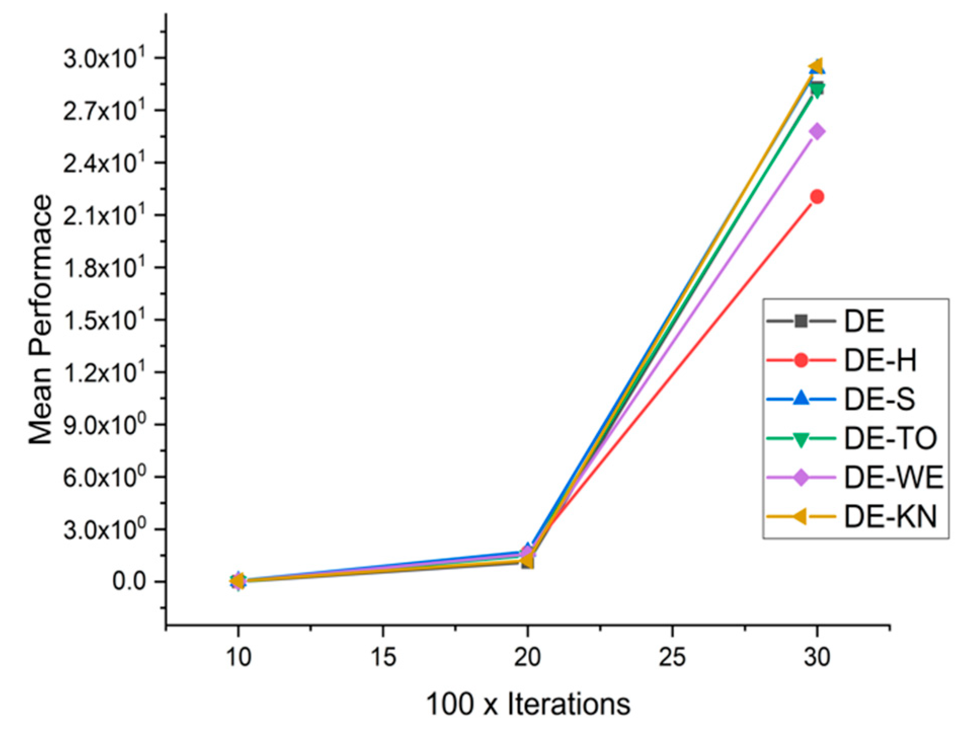
5.5. Results and Graphs on DE Approaches

| Functions | DIM × Iter | DE | DE-H | DE-S | DE-TO | DE-WE | DE-KN |
|---|---|---|---|---|---|---|---|
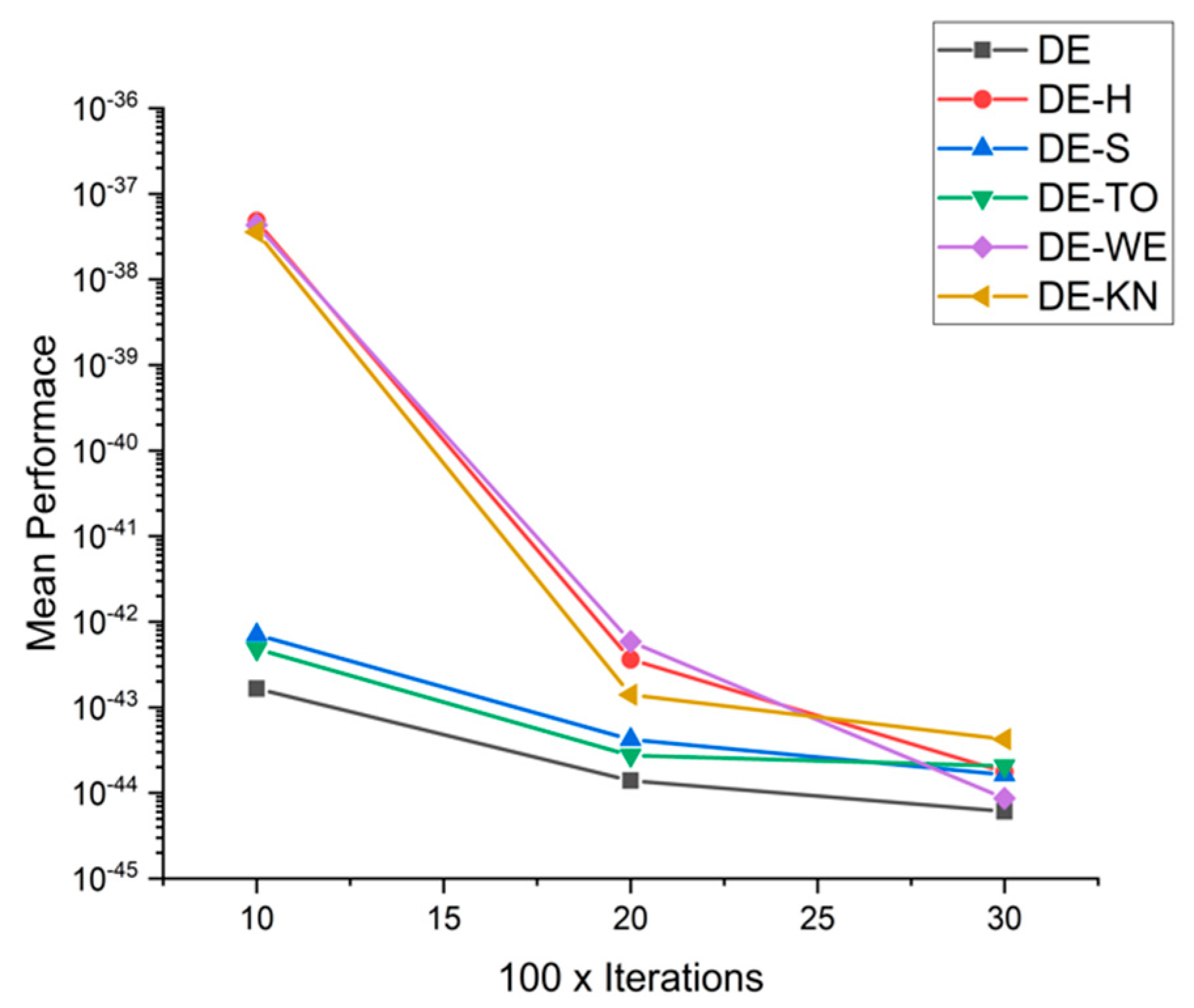
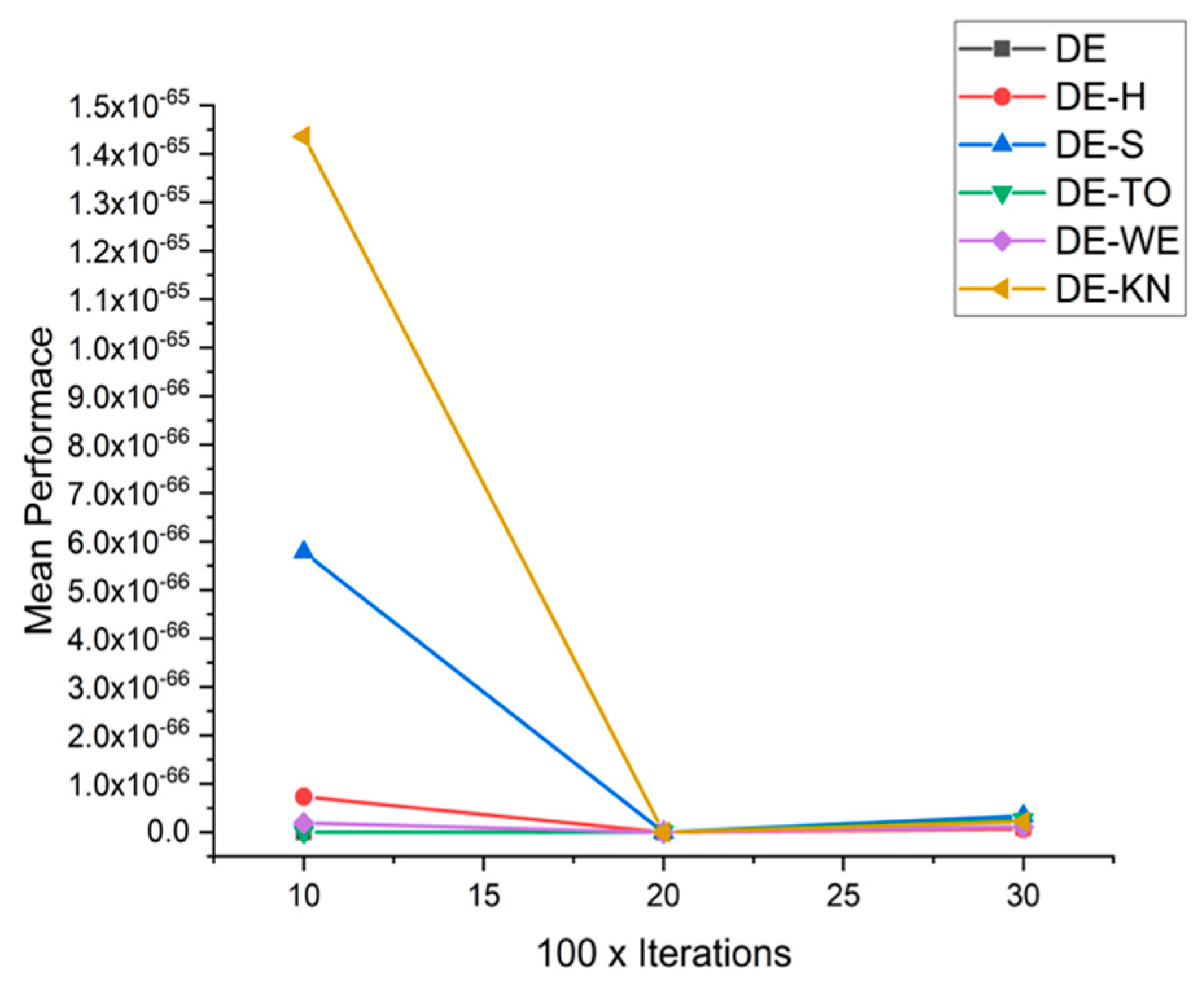
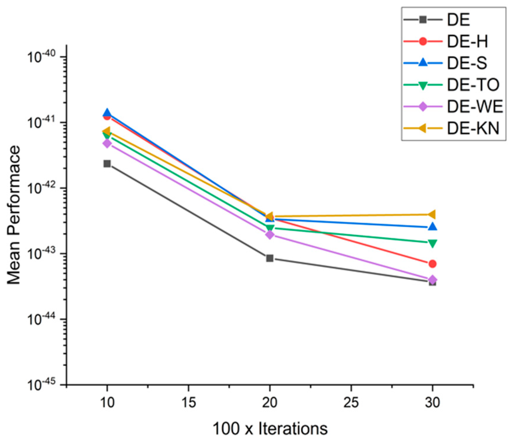
| F1 | 10 × 1000 | 1.1464 × 10−44 | 2.1338 × 10−44 | 5.8561 × 10−44 | 7.4117 × 10−45 | 7.4827 × 10−39 | 5.7658 × 10−39 |
| 20 × 2000 | 3.3550 × 10−46 | 7.2338 × 10−46 | 1.3545 × 10−45 | 1.2426 × 10−45 | 9.6318 × 10−45 | 7.1501 × 10−45 | |
| 30 × 3000 | 8.8946 × 10−47 | 1.2273 × 10−45 | 9.4228 × 10−46 | 1.6213 × 10−46 | 6.2007 × 10−46 | 5.7425 × 10−46 | |
| F2 | 10 × 1000 | 0.0000 × 10+00 | 0.0000 × 10+00 | 0.0000 × 10+00 | 0.0000 × 10+00 | 0.0000 × 10+00 | 0.0000 × 10+00 |
| 20 × 2000 | 0.0000 × 10+00 | 0.0000 × 10+00 | 0.0000 × 10+00 | 0.0000 × 10+00 | 0.0000 × 10+00 | 0.0000 × 10+00 | |
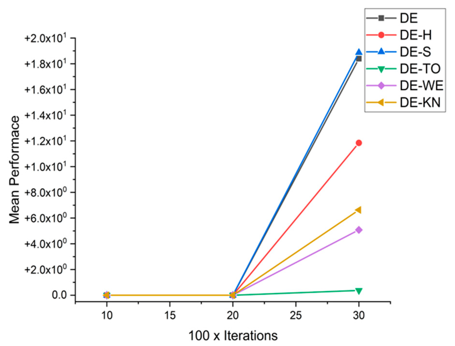
| 30 × 3000 | 1.8392 × 10+01 | 1.1846 × 10+01 | 1.8871 × 10+01 | 3.7132 × 10−01 | 5.0821 × 10+00 | 6.6313 × 10+00 | |
| F3 | 10 × 1000 | 5.00325 × 10−44 | 1.5019 × 10−38 | 9.3956 × 10−44 | 4.7807 × 10−44 | 1.6251 × 10−38 | 1.3411 × 10−38 |
| 20 × 2000 | 2.56987 × 10−45 | 4.1485 × 10−44 | 1.5339 × 10−44 | 3.0262 × 10−45 | 9.5984 × 10−44 | 1.3606 × 10−43 | |
| 30 × 3000 | 1.01692 × 10−45 | 2.7349 × 10−45 | 4.0581 × 10−45 | 4.5726 × 10−45 | 4.5686 × 10−45 | 5.4659 × 10−45 | |
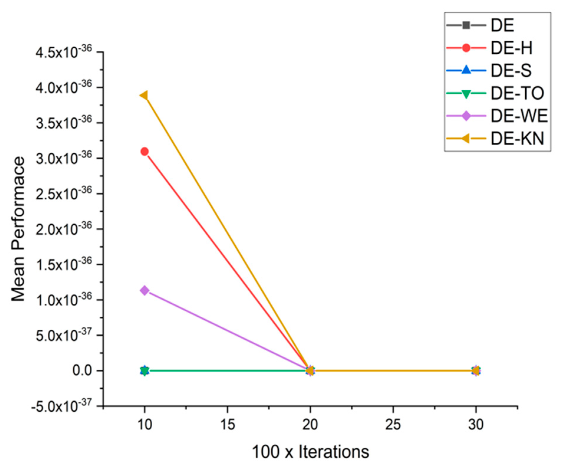
| F4 | 10 × 1000 | 5.81825 × 10−42 | 3.0950 × 10−36 | 2.2300 × 10−41 | 1.6903 × 10−41 | 1.1331 × 10−36 | 3.8869 × 10−36 |
| 20 × 2000 | 2.70747 × 10−43 | 1.0658 × 10−41 | 1.6730 × 10−42 | 1.3490 × 10−42 | 1.3094 × 10−41 | 6.0053 × 10−42 | |
| 30 × 3000 | 2.99887 × 10−43 | 1.4032 × 10−42 | 4.4442 × 10−42 | 5.9186 × 10−43 | 4.6922 × 10−43 | 1.4829 × 10−42 | |
| F5 | 10 × 1000 | 1.65318 × 10−43 | 4.7939 × 10−38 | 7.0329 × 10−43 | 4.8106 × 10−43 | 4.3219 × 10−38 | 3.5770 × 10−38 |
| 20 × 2000 | 1.39082 × 10−44 | 3.6325 × 10−43 | 4.2191 × 10−44 | 2.7448 × 10−44 | 5.8557 × 10−43 | 1.4008 × 10−43 | |
| 30 × 3000 | 6.07162 × 10−45 | 1.7557 × 10−44 | 1.6295 × 10−44 | 2.0582 × 10−44 | 8.6773 × 10−45 | 4.2285 × 10−44 | |
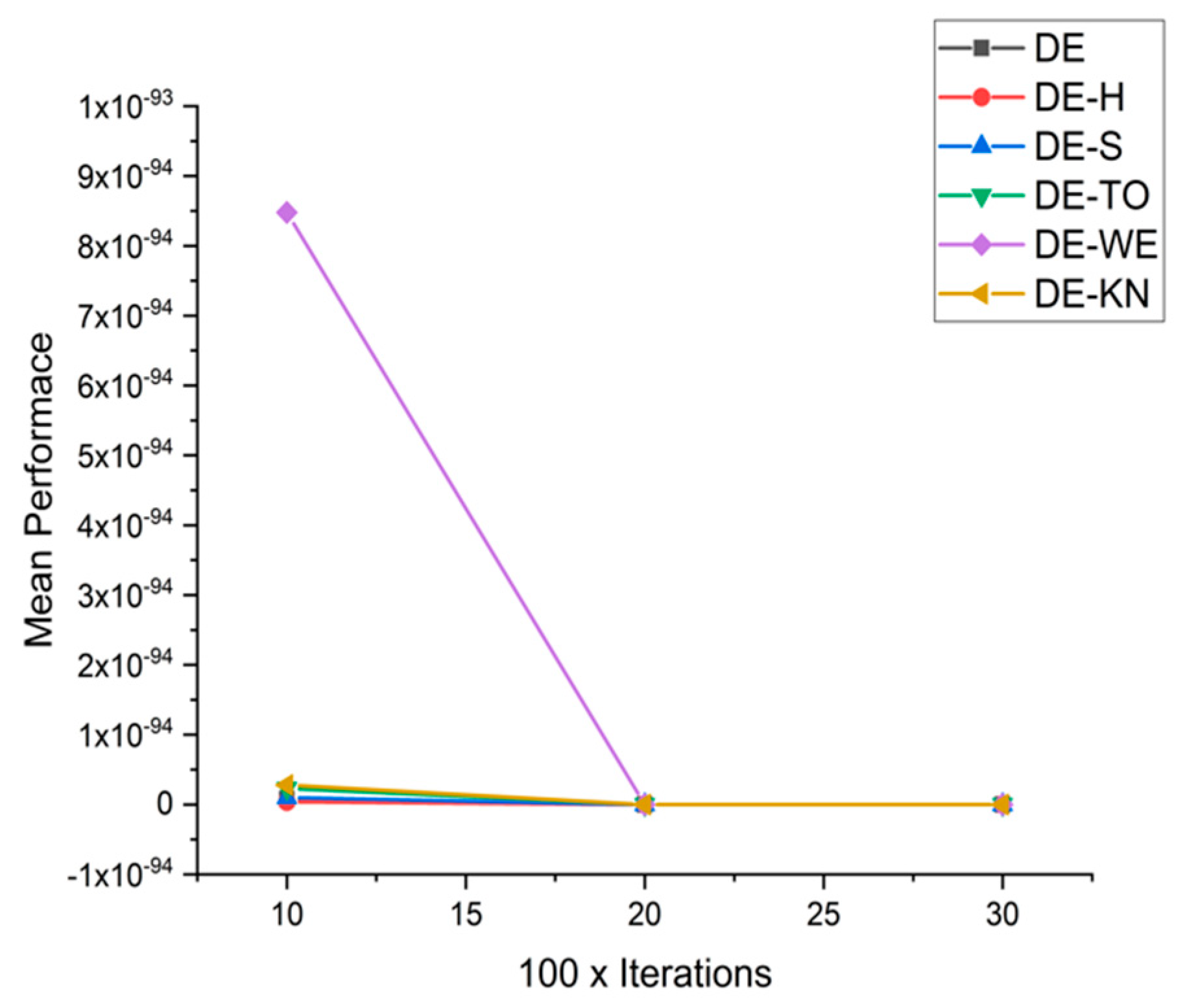
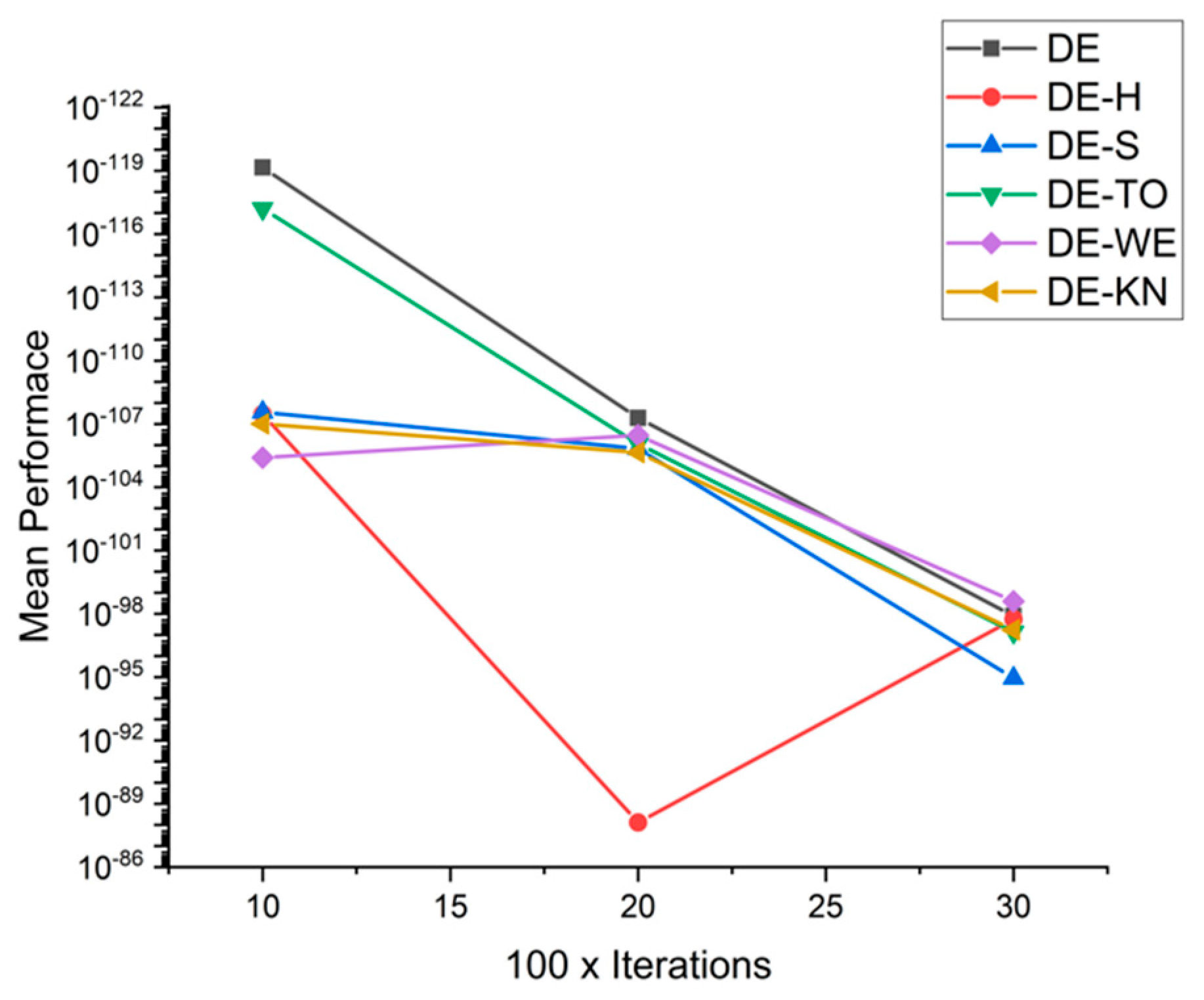
| F6 | 10 × 1000 | 7.8201 × 10−96 | 3.8819 × 10−96 | 9.7956 × 10−96 | 2.3292 × 10−95 | 8.4774 × 10−94 | 2.8037 × 10−95 |
| 20 × 2000 | 1.6847 × 10−125 | 8.6880 × 10−124 | 5.9005 × 10−122 | 8.7800 × 10−123 | 3.7438 × 10−124 | 1.3947 × 10−124 | |
| 30 × 3000 | 2.4533 × 10−140 | 1.5487 × 10−139 | 5.7211 × 10−138 | 4.4492 × 10−137 | 6.5749 × 10−140 | 3.4442 × 10−137 | |
| F7 | 10 × 1000 | 8.0217 × 10−75 | 7.3243 × 10−67 | 5.7807 × 10−66 | 1.0243 × 10−73 | 1.9035 × 10−67 | 1.4359 × 10−65 |
| 20 × 2000 | 4.0682 × 10−71 | 1.5037 × 10−70 | 1.5747 × 10−69 | 1.0623 × 10−70 | 5.5546 × 10−70 | 2.3507 × 10−70 | |
| 30 × 3000 | 8.5895 × 10−68 | 6.6009 × 10−68 | 3.3919 × 10−67 | 2.6036 × 10−67 | 1.1587 × 10−67 | 2.1901 × 10−67 | |
| F8 | 10 × 1000 | 7.0221 × 10−120 | 3.4271 × 10−108 | 2.7718 × 10−108 | 6.3092 × 10−118 | 3.9423 × 10−106 | 9.9394 × 10−108 |
| 20 × 2000 | 5.2096 × 10−108 | 7.7158 × 10−89 | 1.4732 × 10−106 | 8.8720 × 10−107 | 3.4490 × 10−107 | 2.2539 × 10−106 | |
| 30 × 3000 | 1.2538 × 10−98 | 1.8071 × 10−98 | 1.1085 × 10−95 | 7.2462 × 10−98 | 2.5375 × 10−99 | 5.8040 × 10−98 | |
| F9 | 10 × 1000 | 0.0000 × 10+00 | 0.0000 × 10+00 | 0.0000 × 10+00 | 0.0000 × 10+00 | 0.0000 × 10+00 | 0.0000 × 10+00 |
| 20 × 2000 | 0.0000 × 10+00 | 0.0000 × 10+00 | 0.0000 × 10+00 | 0.0000 × 10+00 | 0.0000 × 10+00 | 0.0000 × 10+00 | |
| 30 × 3000 | 0.0000 × 10+00 | 0.0000 × 10+00 | 0.0000 × 10+00 | 0.0000 × 10+00 | 0.0000 × 10+00 | 0.0000 × 10+00 | |
| F10 | 10 × 1000 | 1.3459 × 10−75 | 2.6493 × 10−66 | 2.6884 × 10−66 | 3.6168 × 10−67 | 3.8397 × 10−67 | 1.8408 × 10−66 |
| 20 × 2000 | 3.0478 × 10−71 | 1.6106 × 10−69 | 5.5253 × 10−69 | 2.7746 × 10−70 | 5.3662 × 10−70 | 5.0931 × 10−70 | |
| 30 × 3000 | 8.2514 × 10−68 | 1.0937 × 10−66 | 4.1120 × 10−67 | 1.3055 × 10−67 | 3.5397 × 10−68 | 6.0736 × 10−67 | |
| F11 | 10 × 1000 | 2.3417 × 10−42 | 1.2483 × 10−41 | 1.3726 × 10−41 | 6.3337 × 10−42 | 4.8161 × 10−42 | 7.3464 × 10−42 |
| 20 × 2000 | 8.4769 × 10−44 | 3.5140 × 10−43 | 3.3777 × 10−43 | 2.4721 × 10−43 | 1.9553 × 10−43 | 3.6961 × 10−43 | |
| 30 × 3000 | 3.6888 × 10−44 | 6.9938 × 10−44 | 2.5123 × 10−43 | 1.4710 × 10−43 | 4.0019 × 10−44 | 3.9503 × 10−43 | |
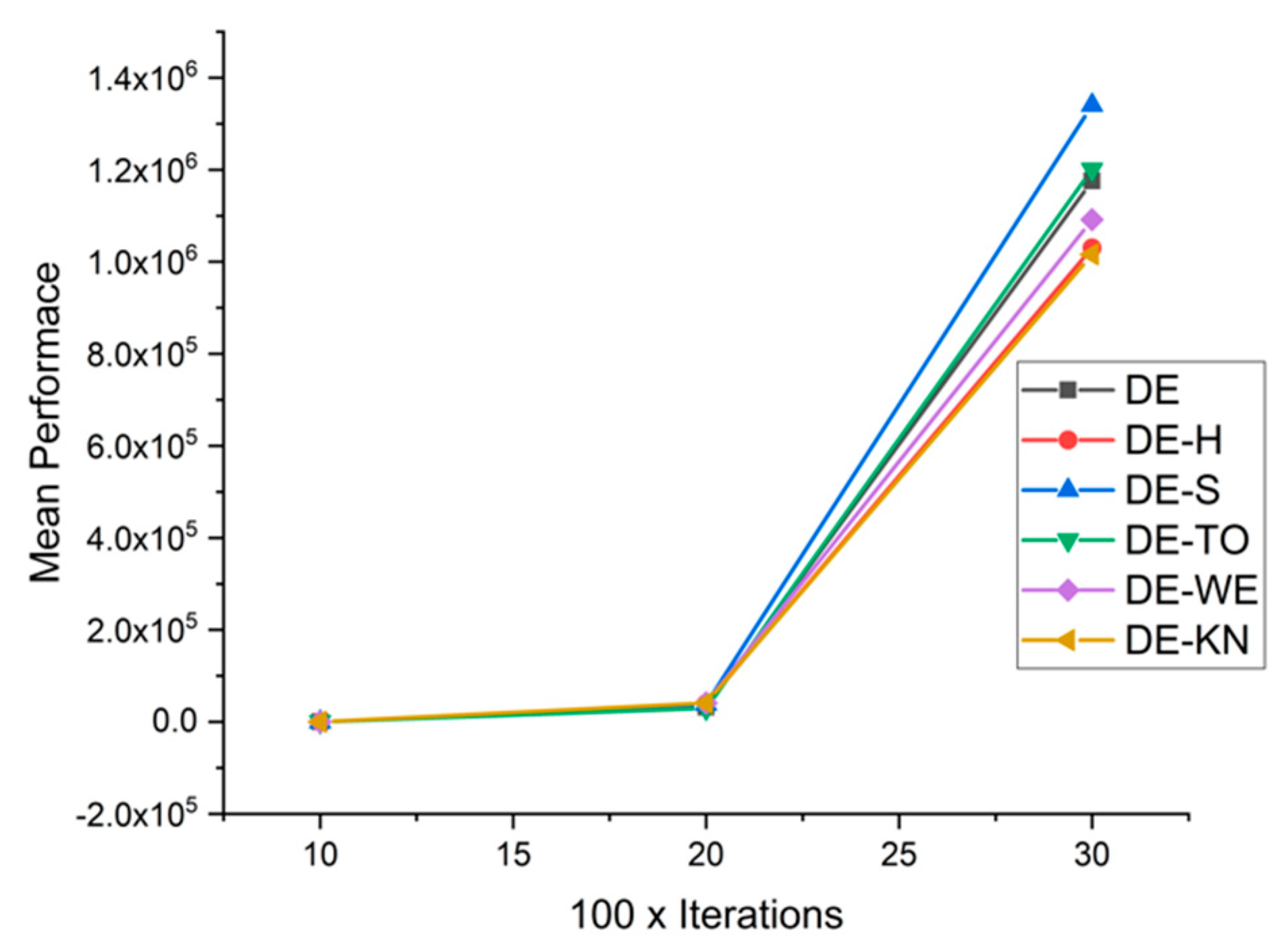
| F12 | 10 × 1000 | 2.3304 × 10+00 | 4.4354 × 10+00 | 3.4520 × 10+00 | 5.1229 × 10+00 | 3.8782 × 10+00 | 2.7840 × 10+00 |
| 20 × 2000 | 3.1768 × 10+04 | 3.9596 × 10+04 | 3.8814 × 10+04 | 2.9488 × 10+04 | 4.1181 × 10+04 | 4.0914 × 10+04 | |
| 30 × 3000 | 1.1760 × 10+06 | 1.0300 × 10+06 | 1.3402 × 10+06 | 1.2008 × 10+06 | 1.0916 × 10+06 | 1.0160 × 10+06 | |
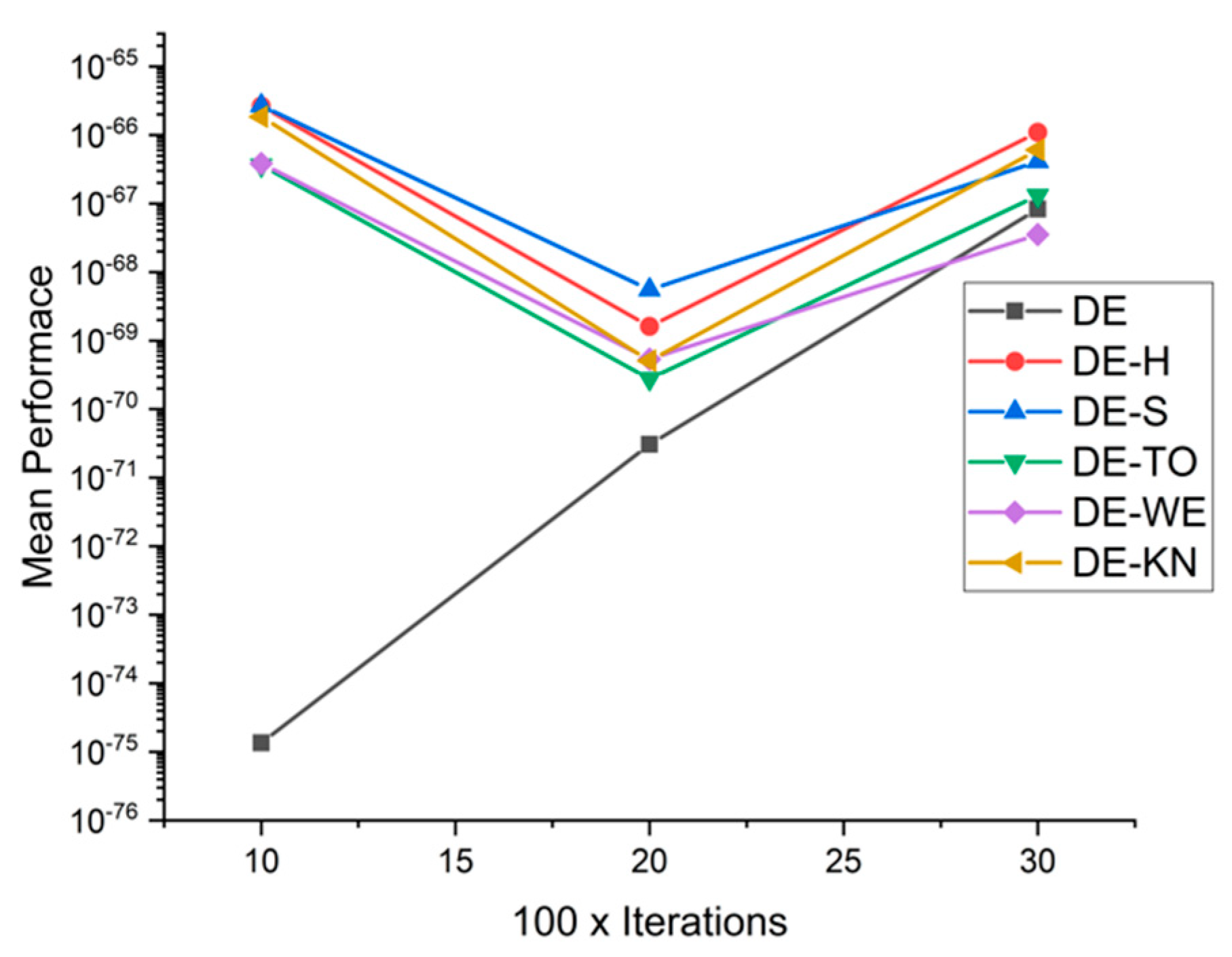
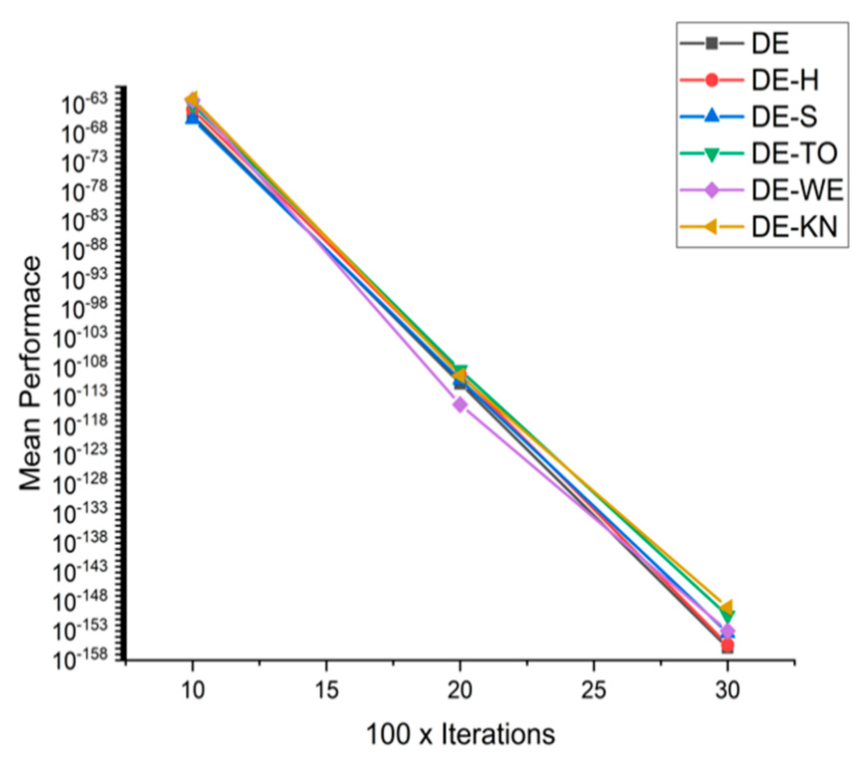
| F13 | 10 × 1000 | 1.3940 × 10−65 | 1.3756 × 10−64 | 3.1956 × 10−66 | 9.3609 × 10−64 | 5.4864 × 10−63 | 9.2695 × 10−63 |
| 20 × 2000 | 2.0163 × 10−111 | 8.5333 × 10−110 | 8.5260 × 10−111 | 3.9836 × 10−109 | 5.0102 × 10−115 | 4.4624 × 10−110 | |
| 30 × 3000 | 1.4146 × 10−156 | 4.3434 × 10−156 | 4.4702 × 10−154 | 4.3862 × 10−151 | 1.0781 × 10−153 | 1.0142 × 10−149 | |
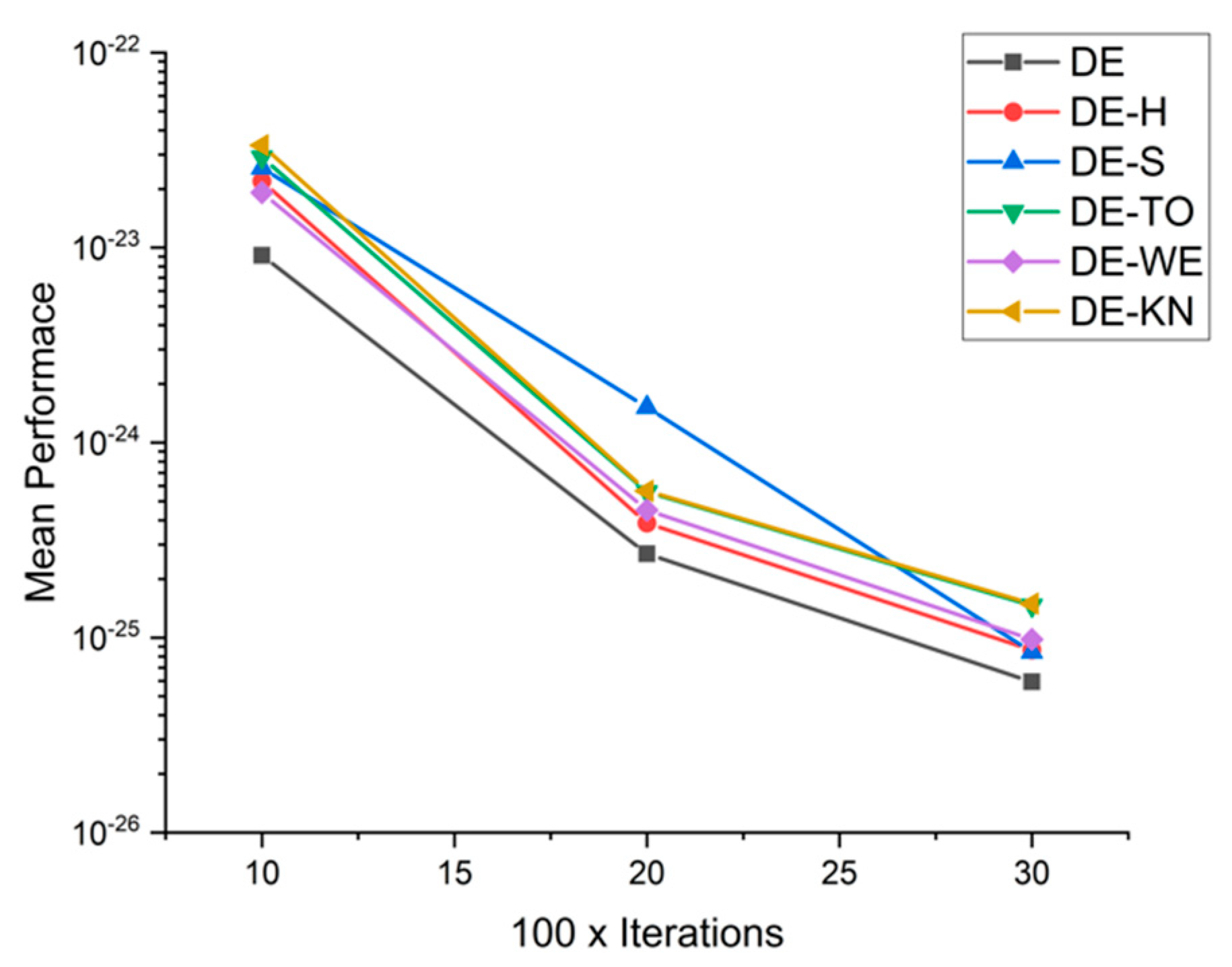
| F14 | 10 × 1000 | 9.1259 × 10⁻²⁴ | 2.1900 × 10⁻²³ | 2.5559 × 10⁻²³ | 2.9039 × 10⁻²³ | 1.9174 × 10⁻²³ | 3.3427 × 10⁻²³ |
| 20 × 2000 | 2.6867 × 10⁻²⁵ | 3.8631 × 10⁻²⁵ | 1.5177 × 10⁻²⁴ | 5.5714 × 10⁻²⁵ | 4.5049 × 10⁻²⁵ | 5.6503 × 10⁻²⁵ | |
| 30 × 3000 | 5.9241 × 10⁻²⁶ | 8.6401 × 10⁻²⁶ | 8.4348 × 10⁻²⁶ | 1.4630 × 10⁻²⁵ | 9.7932 × 10⁻²⁶ | 1.4921 × 10⁻²⁵ | |
| F15 | 10 × 1000 | 1.0493 × 10−185 | 4.0276 × 10−181 | 5.0331 × 10−182 | 3.1770 × 10−183 | 1.1698 × 10−180 | 2.6563 × 10−182 |
| 20 × 2000 | 2.9407 × 10−159 | 9.9152 × 10−159 | 2.1401 × 10−158 | 9.0345 × 10−156 | 3.8871 × 10−158 | 8.0144 × 10−160 | |
| 30 × 3000 | 4.6769 × 10−138 | 1.0737 × 10−137 | 7.0544 × 10−138 | 8.0376 × 10−138 | 4.9091 × 10−139 | 1.1054 × 10−137 | |
| F16 | 10 × 1000 | 1.8635 × 10−04 | 1.8109 × 10−02 | 4.9798 × 10−02 | 5.8605 × 10−04 | 1.4858 × 10−02 | 3.7220 × 10−02 |
| 20 × 2000 | 1.1032 × 10+00 | 1.6605 × 10+00 | 1.7157 × 10+00 | 1.4875 × 10+00 | 1.5697 × 10+00 | 1.2008 × 10+00 | |
| 30 × 3000 | 2.8283 × 10+01 | 2.2049 × 10+01 | 2.9388 × 10+01 | 2.8205 × 10+01 | 2.5794 × 10+01 | 2.9526 × 10+01 |
5.6. Friedman and Kruskal–Wallis Test on DE Approaches
| Friedman Value | Kruskal-Wallis | |
|---|---|---|
| DE | 63.74 | 65.11 |
| DE-H | 59.31 | 60.41 |
| DE-S | 64.01 | 65.05 |
| DE-TO | 63.76 | 65.35 |
| DE-WE | 63.35 | 63.93 |
| DE-KN | 63.33 | 64.06 |
6. Comparison of PSO and DE Regarding Data Classification
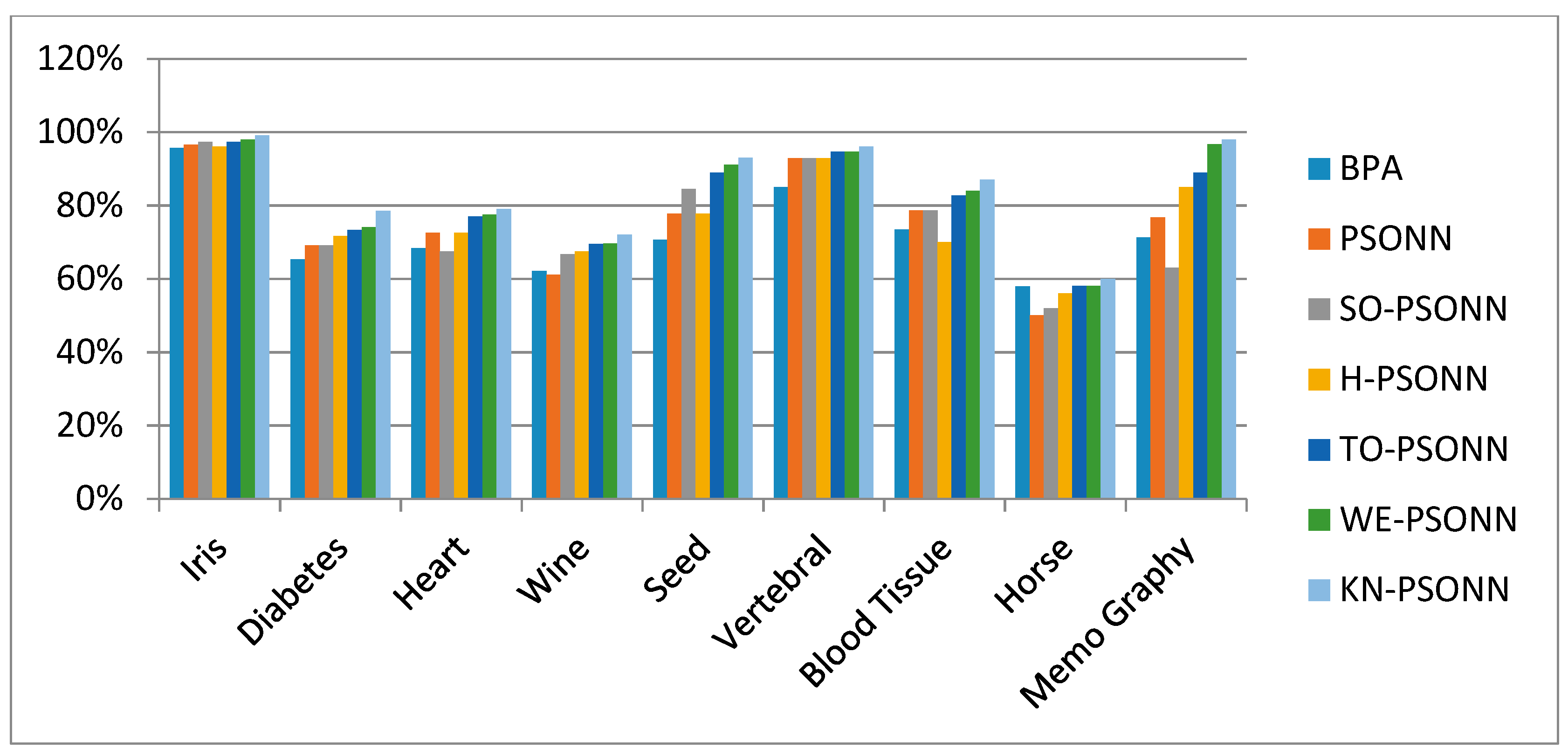
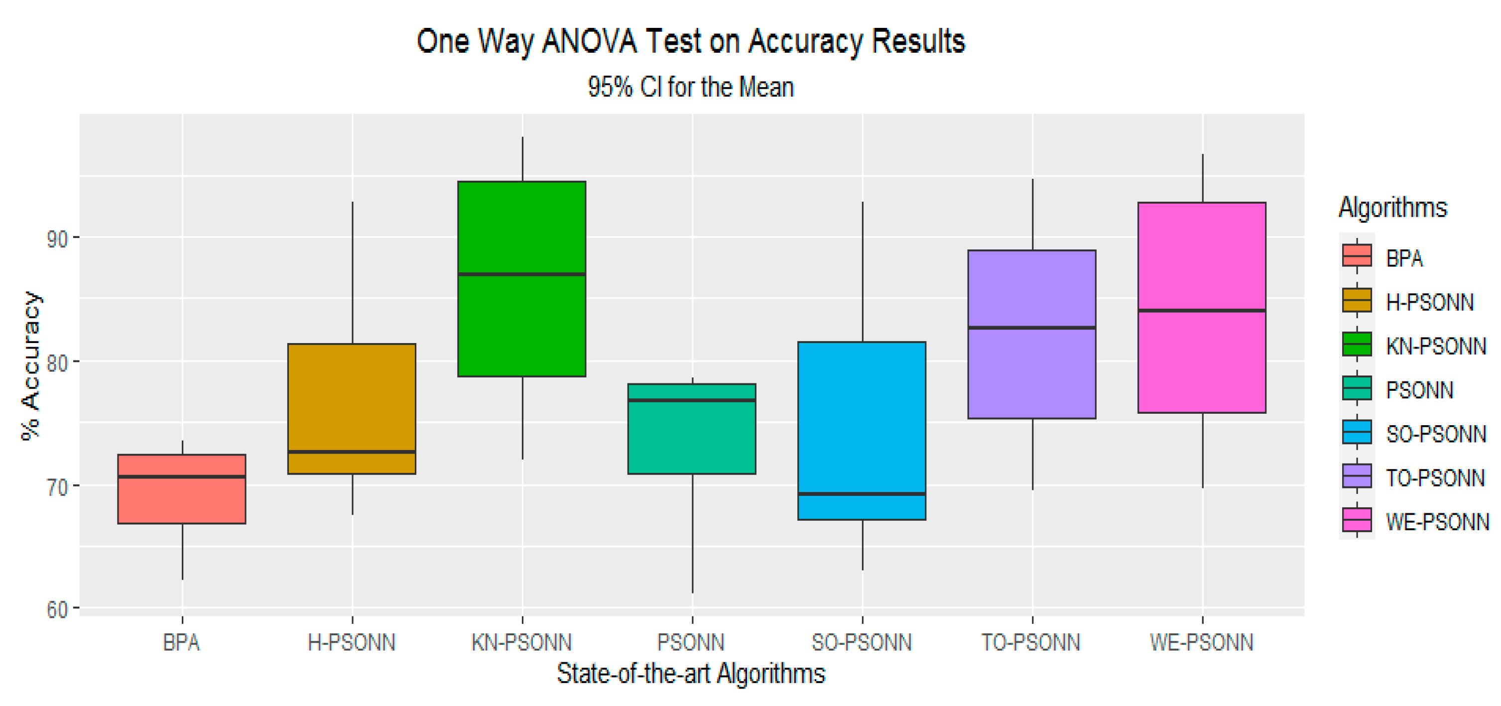
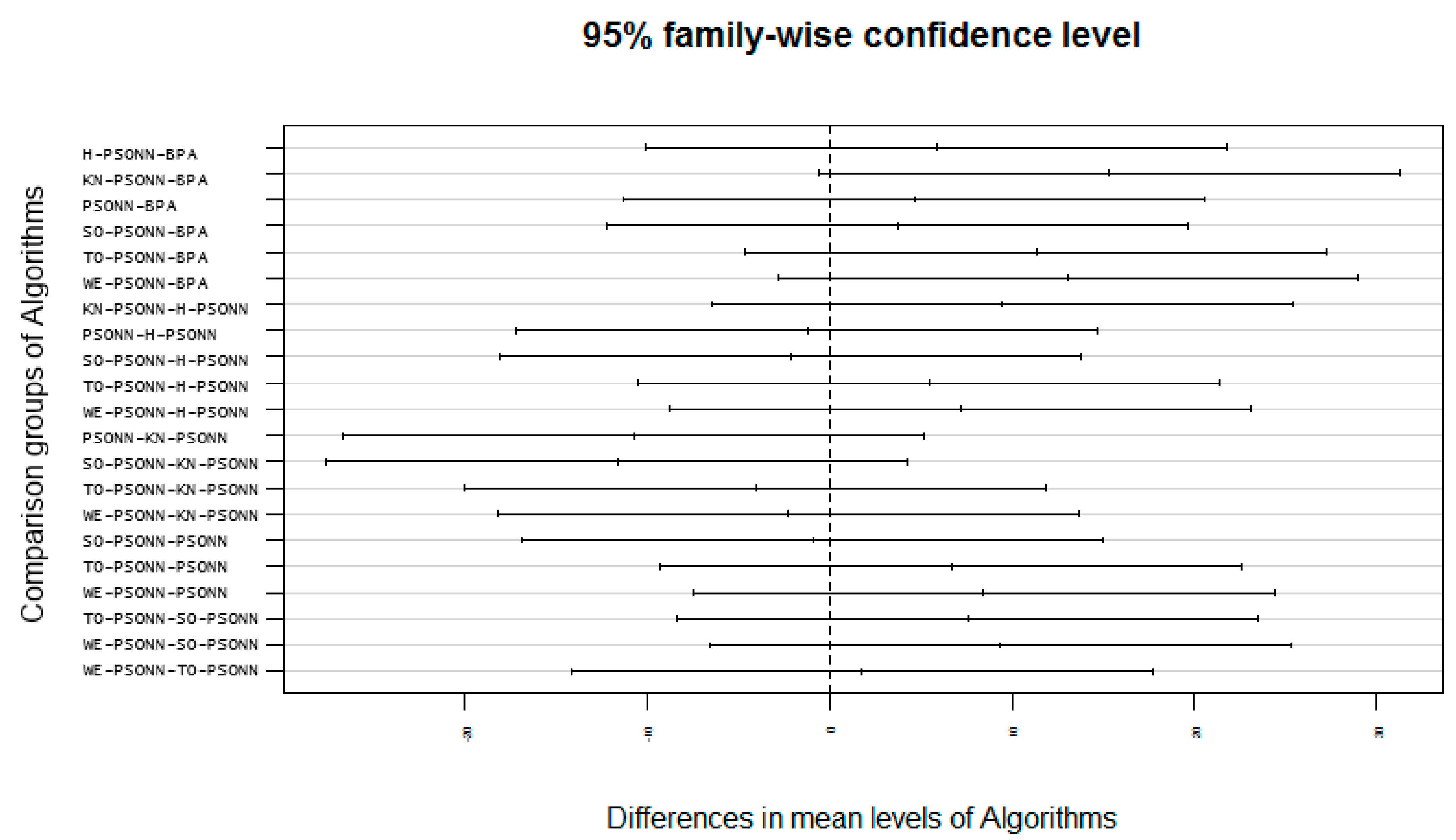
6.1. NN Classifications with PSO-Based Initialization Approaches
Discussion
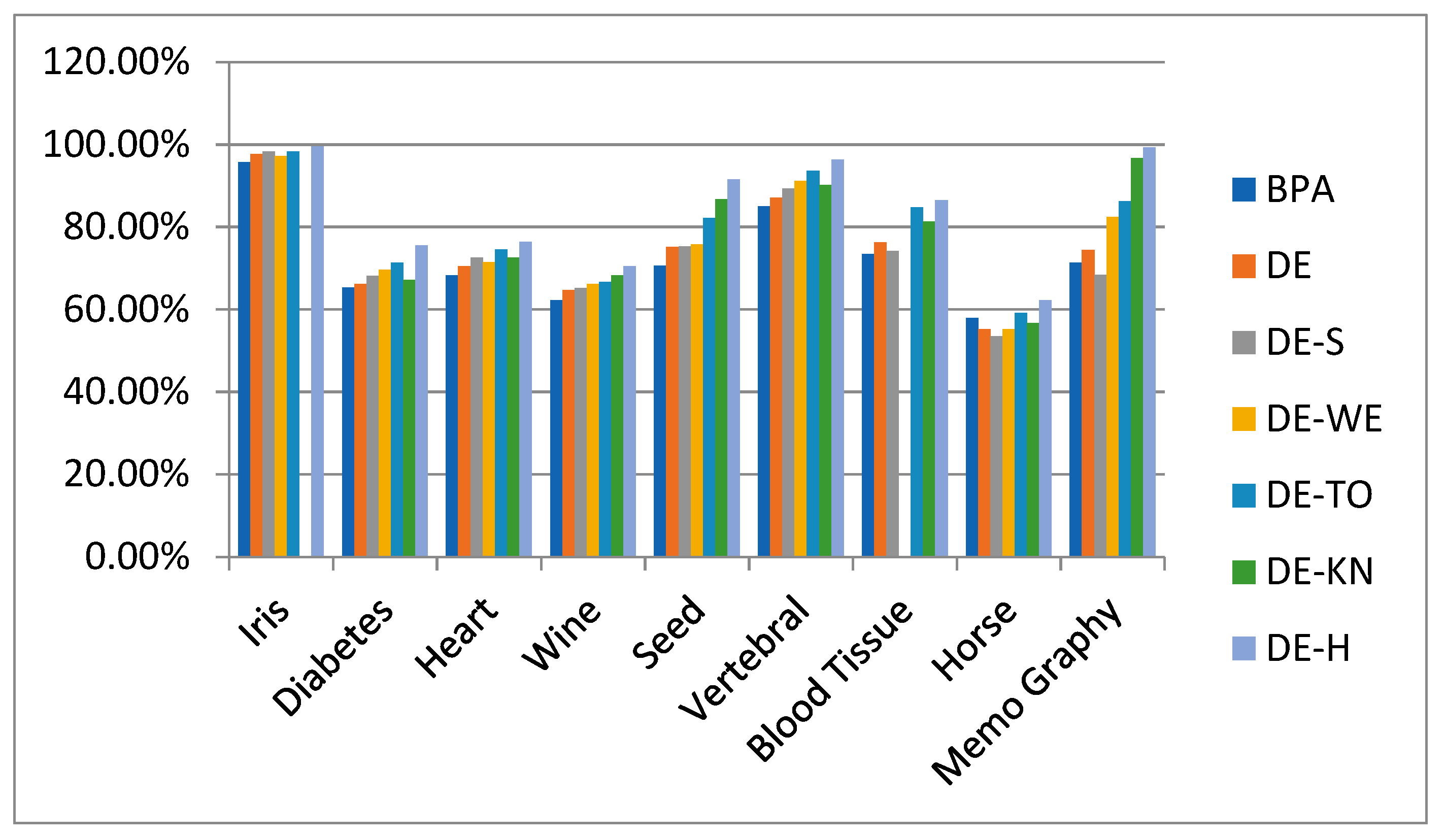
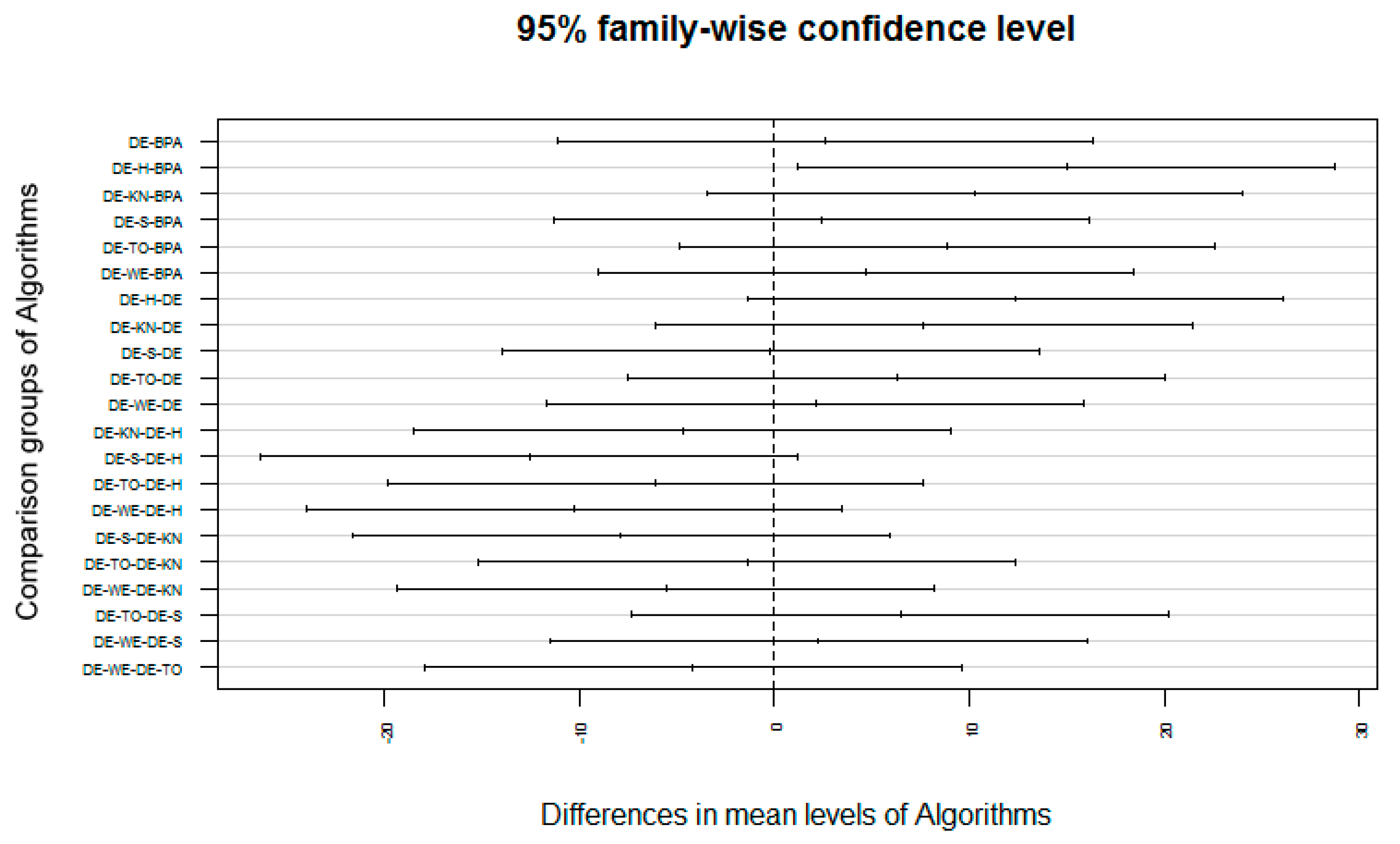
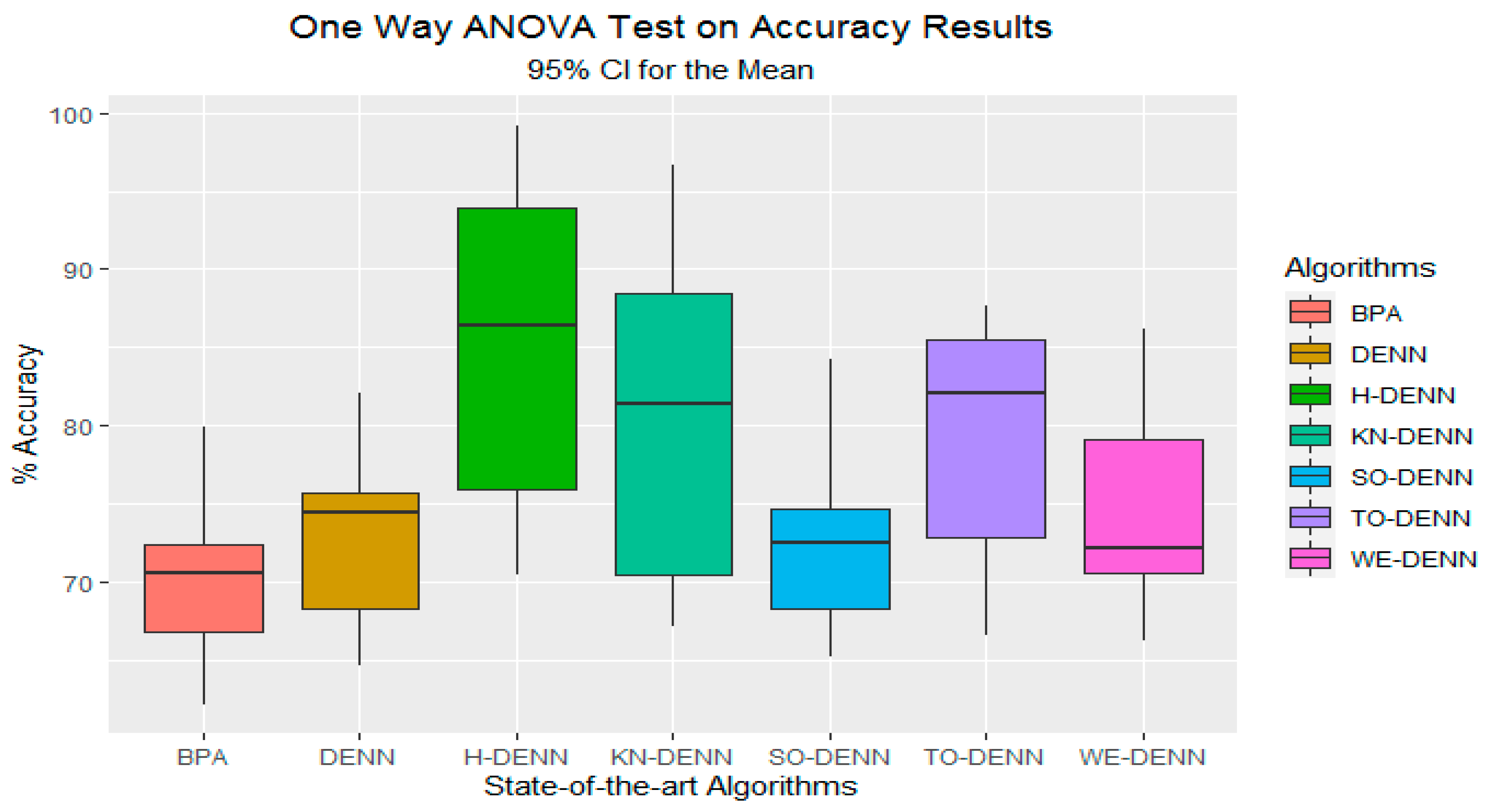
6.2. NN Classifications with DE-Based Initialization Approaches
Discussion
7. Conclusions
Author Contributions
Funding
Institutional Review Board Statement
Informed Consent Statement
Data Availability Statement
Conflicts of Interest
References
- Yang, C.H.; Chang, H.W.; Ho, C.H.; Chou, Y.C.; Chuang, L.Y. Conserved PCR primer set designing for closely-related species to complete mitochondrial genome sequencing using a sliding window-based PSO algorithm. PLoS ONE 2011, 6, e17729. [Google Scholar] [CrossRef] [Green Version]
- Mahi, M.; Baykan, Ö.K.; Kodaz, H. A new hybrid method based on particle swarm optimization, ant colony optimization and 3-opt algorithms for traveling salesman problem. Appl. Soft Comput. 2015, 30, 484–490. [Google Scholar] [CrossRef]
- Rao, S.S. Engineering Optimization: Theory and Practice; John Wiley & Sons: Hoboken, NJ, USA, 2019. [Google Scholar]
- Zhang, G.; Lu, J.; Gao, Y. Multi-Level Decision Making: Models, Methods and Applications. 2015. Available online: https://0-www-springer-com.brum.beds.ac.uk/gp/book/9783662460580 (accessed on 15 April 2021).
- Beni, G.; Wang, J. Swarm Intelligence in Cellular Robotic Systems, in Robots and Biological Systems: Towards a New Bionics? Springer: New York, NY, USA, 1993; pp. 703–712. [Google Scholar]
- Acharya, J.; Mehta, M.; Saini, B. Particle swarm optimization based load balancing in cloud computing. In Proceedings of the 2016 International Conference on Communication and Electronics Systems (ICCES), Coimbatore, India, 21–22 October 2016. [Google Scholar]
- Zhang, Y.; Xiong, X.; Zhang, Q.D. An improved self-adaptive PSO algorithm with detection function for multimodal function optimization problems. Math. Probl. Eng. 2013, 2013, 1–8. Available online: https://econpapers.repec.org/article/hinjnlmpe/716952.htm (accessed on 15 April 2021). [CrossRef]
- Eberhart, R.; Kennedy, J. Particle swarm optimization. In Proceedings of the IEEE International Conference on Neural Networks, Perth, WA, Australia, 27 November–1 December 1995; pp. 1942–1948. [Google Scholar]
- Yang, X.-S. A new metaheuristic bat-inspired algorithm. In Nature Inspired Cooperative Strategies for Optimization (NICSO 2010); Springer: New York, NY, USA, 2010; pp. 65–74. [Google Scholar]
- Dorigo, M.; Di Caro, G. Ant colony optimization: A new meta-heuristic. In Proceedings of the 1999 Congress on Evolutionary Computation—CEC99, Washington, DC, USA, 6–9 July 1999; pp. 1470–1477, Cat. No. 99TH8406. [Google Scholar]
- Pham, D.T.; Ghanbarzadeh, A.; Koç, E.; Otri, S.; Rahim, S.; Zaidi, M. The bees algorithm—A novel tool for complex optimisation problems. In Intelligent Production Machines and Systems; Elsevier: Amsterdam, The Netherlands, 2006; pp. 454–459. [Google Scholar]
- Poli, R.; Kennedy, J.; Blackwell, T. Particle Swarm Optimization; Springer: New York, NY, USA, 2007; Volume 1, pp. 33–57. [Google Scholar]
- Bai, Q. Analysis of particle swarm optimization algorithm. Comput. Inf. Sci. 2010, 3, 180. [Google Scholar] [CrossRef] [Green Version]
- AlRashidi, M.R.; El-Hawary, M.E. A survey of particle swarm optimization applications in electric power systems. IEEE Trans. Evol. Comput. 2008, 13, 913–918. [Google Scholar] [CrossRef]
- Zhu, H.M.; Wu, Y.P. A PSO algorithm with high speed convergence. Control Decis. 2010, 25, 20–24. [Google Scholar]
- Chen, B.; Lei, H.; Shen, H.; Liu, Y.; Lu, Y. A hybrid quantum-based PIO algorithm for global numerical optimization. Sci. China Inf. Sci. 2019, 62, 1–12. [Google Scholar] [CrossRef] [Green Version]
- Shi, Y. Particle swarm optimization: Developments, applications and resources. In Proceedings of the 2001 Congress on Evolutionary Computation, Washington, DC, USA, 6–9 July 1999; pp. 81–86, Cat. No. 01TH8546. [Google Scholar]
- Chen, S.; Montgomery, J. Particle swarm optimization with thresheld convergence. In Proceedings of the 2013 IEEE Congress on Evolutionary Computation, Cancun, Mexico, 20–23 June 2013; pp. 510–516. [Google Scholar]
- Alam, M.N.; Das, B.; Pant, V. A comparative study of metaheuristic optimization approaches for directional overcurrent relays coordination. Electr. Power Syst. Res. 2015, 128, 39–52. [Google Scholar] [CrossRef]
- Lu, Z.; Hou, Z. Adaptive Mutation PSO Algorithm. Acta Electronca Sinica 3 2004, 32, 417–420. [Google Scholar]
- Rashedi, E.; Nezamabadi-Pour, H.; Saryazdi, S. GSA: A Gravitational Search Algorithm; Elsevier: Amsterdam, The Netherlands, 2009; Volume 179, pp. 2232–2248. [Google Scholar]
- Li, X.; Zhuang, J.; Wang, S.; Zhang, Y. A particle swarm optimization algorithm based on adaptive periodic mutation. In Proceedings of the 2008 Fourth International Conference on Natural Computation, Jinan, China, 18–20 October 2008; pp. 150–155. [Google Scholar]
- Song, M.-P.; Gu, G.-C. Research on particle swarm optimization: A review. In Proceedings of the 2004 International Conference on Machine Learning and Cybernetics, Shanghai, China, 26–29 August 2004; pp. 2236–2241, Cat. No. 04EX826. [Google Scholar]
- Maaranen, H.; Miettinen, K.; Penttinen, A. On Initial Populations of a Genetic Algorithm for Continuous Optimization Problems; Springer: New York, NY, USA, 2007; Volume 37, pp. 405–436. [Google Scholar]
- Pant, M.; Thangaraj, R.; Grosan, C.; Abraham, A. Improved particle swarm optimization with low-discrepancy sequences. In Proceedings of the 2008 IEEE Congress on Evolutionary Computation (IEEE World Congress on Computational Intelligence), Hong Kong, China, 1–6 June 2008; pp. 3011–3018. [Google Scholar]
- Parsopoulos, K.E.; Vrahatis, M.N. Initializing the particle swarm optimizer using the nonlinear simplex method. Adv. Intell. Syst. Fuzzy Syst. Evol. Comput. 2002, 216, 1–6. [Google Scholar]
- Richards, M.; Ventura, D. Choosing a starting configuration for particle swarm optimization. Neural Netw. 2004, 25, 2309–2312. [Google Scholar]
- Nguyen, X.H.; Nguyen, Q.U.; McKay, R.I. PSO with randomized low-discrepancy sequences. In Proceedings of the 9th Annual Conference on Genetic and Evolutionary Computation—GECCO ’07, New York, NY, USA, 7–11 July 2007; p. 173. [Google Scholar]
- Uy, N.Q.; Hoai, N.X.; McKay, R.I.; Tuan, P.M. Initialising PSO with randomised low-discrepancy sequences: The comparative results. In Proceedings of the 2007 IEEE Congress on Evolutionary Computation, Singapore, 25–28 September 2007; pp. 1985–1992. [Google Scholar]
- Thangaraj, R.; Pant, M.; Deep, K. Initializing PSO with probability distributions and low-discrepancy sequences: The comparative results. In Proceedings of the World Congress on Nature & Biologically Inspired Computing (NaBIC), Coimbatore, India, 9–11 December 2009; pp. 1121–1126. [Google Scholar] [CrossRef]
- Thangaraj, R.; Pant, M.; Abraham, A.; Badr, Y. Hybrid Evolutionary Algorithm for Solving Global Optimization Problems. In Proceedings of the International Conference on Hybrid Artificial Intelligence Systems, Salamanca, Spain, 10–12 June 2009. [Google Scholar]
- Pant, M.; Thangaraj, R.; Singh, V.P.; Abraham, A. Particle Swarm Optimization Using Sobol Mutation. In Proceedings of the 2008 First International Conference on Emerging Trends in Engineering and Technology, Nagpur, India, 16–18 July 2008; pp. 367–372. [Google Scholar]
- Du, J.; Zhang, F.; Huang, G.; Yang, J. A new initializing mechanism in Particle Swarm Optimization. In Proceedings of the 2011 IEEE International Conference on Computer Science and Automation Engineering, Shanghai, China, 10–12 June 2011; Volume 4, pp. 325–329. [Google Scholar]
- Murugan, P. Modified particle swarm optimisation with a novel initialisation for finding optimal solution to the transmission expansion planning problem. IET Gener. Transm. Distrib. 2012, 6, 1132–1142. [Google Scholar] [CrossRef]
- Yin, L.; Hu, X.-M.; Zhang, J. Space-based initialization strategy for particle swarm optimization. In Proceedings of the fifteenth Annual Conference Companion on Genetic and Evolutionary Computation Conference Companion—GECCO ’13 Companion, New York, NY, USA, 6–10 July 2013; pp. 19–20. [Google Scholar]
- Jensen, B.; Bouhmala, N.; Nordli, T. A Novel Tangent based Framework for Optimizing Continuous Functions. J. Emerg. Trends Comput. Inf. Sci. 2013, 4. [Google Scholar]
- Shatnawi, M.; Nasrudin, M.F.; Sahran, S. A new initialization technique in polar coordinates for Particle Swarm Optimization and Polar PSO. Int. J. Adv. Sci. Eng. Inf. Technol. 2017, 7, 242. [Google Scholar] [CrossRef]
- Bewoor, L.; Prakash, V.C.; Sapkal, S.U. Evolutionary Hybrid Particle Swarm Optimization Algorithm for Solving NP-Hard No-Wait Flow Shop Scheduling Problems. Algorithms 2017, 10, 121. [Google Scholar] [CrossRef] [Green Version]
- Zhang, J.R.; Zhang, J.; Lok, T.M.; Lyu, M.R. A hybrid particle swarm optimization–back-propagation algorithm for feedforward neural network training. Appl. Math. Comput. 2007, 185, 1026–1037. [Google Scholar] [CrossRef]
- Carvalho, M.; Ludermir, T.B. Particle swarm optimization of neural network architectures and weights. In Proceedings of the 7th International Conference on Hybrid Intelligent Systems (HIS 2007), Kaiserslautern, Germany, 17–19 September 2007; pp. 336–339. [Google Scholar]
- Mohammadi, N.; Mirabedini, S.J. Comparison of particle swarm optimization and backpropagation algorithms for training feed forward neural network. J. Math. Comput. Sci. 2014, 12, 113–123. [Google Scholar] [CrossRef]
- Albeahdili, H.M.; Han, T.; Islam, N.E. Hybrid algorithm for the optimization of training convolutional neural network. Int. J. Adv. Comput. Sci. Appl. 2015, 1, 79–85. [Google Scholar]
- Gudise, V.G.; Venayagamoorthy, G.K. Simplex differential evolution. Acta Polytech. Hung. 2009, 6, 95–115. [Google Scholar]
- Nakib, A.; Daachi, B.; Siarry, P. Hybrid Differential Evolution Using Low-Discrepancy Sequences for Image Segmentation. In Proceedings of the 2012 IEEE 26th International Parallel and Distributed Processing Symposium Workshops & PhD Forum, Shanghai, China, 21–25 May 2012; pp. 634–640. [Google Scholar]
- Tang, L.; Zhao, Y.; Liu, J. An Improved Differential Evolution Algorithm for Practical Dynamic Scheduling in Steelmaking-Continuous Casting Production. IEEE Trans. Evol. Comput. 2013, 18, 209–225. [Google Scholar] [CrossRef]
- Wang, L.; Zeng, Y.; Chen, T. Back propagation neural network with adaptive differential evolution algorithm for time series forecasting. Expert Syst. Appl. 2015, 42, 855–863. [Google Scholar] [CrossRef]
- Hou, Y.; Zhao, L.; Lu, H. Fuzzy neural network optimization and network traffic forecasting based on improved differential evolution. Future Gener. Comput. Syst. 2018, 81, 425–432. [Google Scholar] [CrossRef]
- Panigrahi, S.; Bhoi, A.K.; Karali, Y. A modified differential evolution algorithm trained pi-sigma neural network for pattern classification. Int. J. Soft Comput. Eng. 2013, 3, 133–136. [Google Scholar]
- Matsumoto, M.; Nishimura, T. Mersenne twister: A 623-dimensionally equidistributed uniform pseudo-random number generator. ACM Trans. Model. Comput. Simul. TOMACS 1998, 8, 3–30. [Google Scholar] [CrossRef] [Green Version]
- Sobol’, I. On the distribution of points in a cube and the approximate evaluation of integrals. USSR Comput. Math. Math. Phys. 1967, 7, 86–112. [Google Scholar] [CrossRef]
- Halton, J.H. Algorithm 247: Radical-inverse quasi-random point sequence. Commun. ACM 1964, 7, 701–702. [Google Scholar] [CrossRef]
- Panneton, F.; L’Ecuyer, P.; Matsumoto, M. Improved long-period generators based on linear recurrences modulo 2. ACM Trans. Math. Softw. 2006, 32, 1–16. [Google Scholar] [CrossRef]
- Knuth, D.E. The Art of Computer Programming; Addison-Wesley: Reading, MA, USA, 1973; Volume 2, p. 51. [Google Scholar]
- Williams, H.C.; Nikulin, V.V.; Shafarevich, I.R.; Reid, M. Geometries and Groups. Math. Gaz. 1989, 73, 257. [Google Scholar] [CrossRef]
- Ulusoy, U. Application of ANOVA to image analysis results of talc particles produced by different milling. Powder Technol. 2008, 188, 133–138. [Google Scholar] [CrossRef]


| Parameter | Value | ||
|---|---|---|---|
| Search Space | [−100, 100] | ||
| Dimensions | 10 | 20 | 30 |
| Iterations | 1000 | 2000 | 3000 |
| Population size | 50 | ||
| Number of Runs | 10 |
| Algorithm | Parameters |
|---|---|
| PSO | c1 = c2 = 1.49, w = linearly decreasing |
| DE | 𝐹 ∈ [0.4, 1], 𝐶𝑅 ∈ 0.6 |
| Sr.# | Function Name | Objective Function | Search Space | Optimal Value |
|---|---|---|---|---|
| 01 | Sphere | 0 | ||
| 02 | Rastrigin | 0 | ||
| 03 | Axis parallel hyper-ellipsoid | 0 | ||
| 04 | Rotated hyper ellipsoid | 0 | ||
| 05 | Moved Axis | 0 | ||
| 06 | Sum of different power | 0 | ||
| 07 | ChungReynolds | 0 | ||
| 08 | Csendes | 0 | ||
| 09 | Schaffer | 0 | ||
| 10 | Schumer_Steiglitz | 0 | ||
| 11 | Schwefel | 0 | ||
| 12 | Schwefel1.2 | 0 | ||
| 13 | Schwefel 2.21 | 0 | ||
| 14 | Schwefel 2.22 | 0 | ||
| 15 | Schwefel 2.23 | 0 | ||
| 16 | Zakharov | 0 |
| Functions | DIM × Itr | PSO | SO-PSO | H-PSO | TO-PSO | WE-PSO | KN-PSO |
|---|---|---|---|---|---|---|---|
| Mean | Mean | Mean | Mean | Mean | Mean | ||
| F1 | 10 × 1000 | 2.33 × 10−74 | 2.74 × 10−76 | 3.10 × 10−77 | 5.57 × 10−78 | 5.91 × 10−78 | 0.0000 × 10+00 |
| 20 × 2000 | 1.02 × 10−84 | 8.20 × 10−88 | 1.76 × 10−90 | 1.30 × 10−90 | 4.95 × 10−90 | 3.14001 × 10−217 | |
| 30 × 3000 | 1.77 × 10⁻²⁶ | 7.67 × 10⁻²⁰ | 4.13 × 10⁻³² | 1.25 × 10−51 | 1.30 × 10−42 | 8.91595 × 10−88 | |
| F2 | 10 × 1000 | 4.97 × 10−01 | 4.97 × 10−01 | 7.96 × 10−01 | 3.98 × 10−01 | 2.98 × 10−01 | −8602.02 |
| 20 × 2000 | 8.17 × 10+00 | 6.47 × 10+00 | 3.58 × 10+00 | 2.89 × 10+00 | 3.11 × 10+00 | −31,433.3 | |
| 30 × 3000 | 1.01 × 10+01 | 9.86 × 10+00 | 9.45 × 10+00 | 8.16 × 10+00 | 7.76 × 10+00 | −60,711.8 | |
| F3 | 10 × 1000 | 8.70 × 10−80 | 1.79 × 10−79 | 4.87 × 10−79 | 3.91 × 10−82 | 4.40 × 10−81 | 0.0000 × 10+00 |
| 20 × 2000 | 2.62144 | 7.86432 | 2.62144 | 7.07 × 10−90 | 1.78 × 10−89 | 4.78718 × 10−237 | |
| 30 × 3000 | 2.62 × 10+01 | 1.57 × 10+01 | 1.05 × 10+01 | 7.70 × 10⁻³⁵ | 3.87 × 10−57 | 1.57084 × 10−97 | |
| F4 | 10 × 1000 | 4.46 × 10−147 | 3.86 × 10−147 | 9.78 × 10−145 | 7.29 × 10−148 | 1.24 × 10−150 | 0.0000 × 10+00 |
| 20 × 2000 | 3.14 × 10−155 | 9.27 × 10−154 | 2.75 × 10−159 | 5.14 × 10−158 | 4.96 × 10−159 | 0.0000 × 10+00 | |
| 30 × 3000 | 1.82 × 10−133 | 2.36 × 10−135 | 8.53 × 10−130 | 3.13 × 10−138 | 2.54 × 10−136 | 1.6439 × 10−228 | |
| F5 | 10 × 1000 | 4.35 × 10−79 | 8.95 × 10−79 | 2.43 × 10−78 | 2.04 × 10−80 | 2.20 × 10−80 | 0.0000 × 10+00 |
| 20 × 2000 | 1.31 × 10+01 | 3.93 × 10+01 | 1.31 × 10+01 | 3.54 × 10−89 | 3.12 × 10−89 | 2.39359 × 10−236 | |
| 30 × 3000 | 1.31 × 10+02 | 7.86 × 10+01 | 5.24 × 10+01 | 3.85 × 10⁻³⁴ | 1.94 × 10−56 | 2.9093 × 10−87 | |
| F6 | 10 × 1000 | 1.70 × 10−61 | 4.45 × 10−64 | 7.29 × 10−66 | 2.46 × 10−66 | 4.62 × 10−66 | 3.04226 × 10−318 |
| 20 × 2000 | 3.25 × 10−112 | 4.39 × 10−112 | 5.01 × 10−109 | 2.56 × 10−115 | 4.45 × 10−113 | 8.59557 × 10−277 | |
| 30 × 3000 | 7.21 × 10−135 | 4.10 × 10−124 | 1.51 × 10−134 | 6.22 × 10−137 | 6.96 × 10−135 | 2.33033 × 10−223 | |
| F7 | 10 × 1000 | 2.96 × 10−157 | 2.39 × 10−157 | 1.28 × 10−157 | 4.89 × 10−159 | 2.47 × 10−163 | 0.0000 × 10+00 |
| 20 × 2000 | 8.79 × 10−177 | 1.77 × 10−184 | 3.49 × 10−183 | 3.09 × 10−187 | 3.41 × 10−186 | 0.0000 × 10+00 | |
| 30 × 3000 | 1.23 × 10−82 | 1.25 × 10−116 | 5.99 × 10−130 | 5.01 × 10−135 | 4.60 × 10−134 | 8.03288 × 10−175 | |
| F8 | 10 × 1000 | 4.39 × 10−200 | 1.98 × 10−194 | 4.51 × 10−197 | 1.26 × 10−202 | 8.99 × 10−201 | 4.9228 × 10−67 |
| 20 × 2000 | 1.57 × 10⁻²⁰ | 1.04 × 10−93 | 1.10 × 10−148 | 2.84 × 10−157 | 4.09 × 10−151 | 4.5887 × 10⁻¹⁶ | |
| 30 × 3000 | 1.89 × 10−09 | 4.54 × 10⁻¹⁰ | 1.14 × 10−08 | 1.40 × 10⁻¹⁰ | 1.34 × 10−09 | 2.2334 × 10−08 | |
| F9 | 10 × 1000 | 5.49 × 10−01 | 1.30 × 10−01 | 2.02 × 10−01 | 1.26 × 10−01 | 1.42 × 10−01 | 0.824968 |
| 20 × 2000 | 2.05 × 10+00 | 7.83 × 10−01 | 6.83 × 10−01 | 5.84 × 10−01 | 4.32 × 10−01 | 4.56265 | |
| 30 × 3000 | 1.12 × 10+00 | 9.99 × 10−01 | 9.56 × 10−01 | 9.06 × 10−01 | 9.12 × 10−01 | 7.25675 | |
| F10 | 10 × 1000 | 2.23 × 10−138 | 2.23 × 10−138 | 4.35 × 10−137 | 1.02 × 10−140 | 1.10 × 10−139 | 0.0000 × 10+00 |
| 20 × 2000 | 3.79 × 10−148 | 7.87 × 10−149 | 4.19 × 10−147 | 3.78 × 10−151 | 8.73 × 10−153 | 0.0000 × 10+00 | |
| 30 × 3000 | 4.43 × 10−126 | 7.52 × 10−133 | 1.57 × 10−128 | 2.03 × 10−134 | 1.38 × 10−133 | 2.26229 × 10−221 | |
| F11 | 10 × 1000 | 3.75 × 10−187 | 1.57 × 10−192 | 2.15 × 10−191 | 5.57 × 10−198 | 8.99 × 10−198 | 0.0000 × 10+00 |
| 20 × 2000 | 5.29 × 10−193 | 2.53 × 10−195 | 8.45 × 10−195 | 8.45 × 10−195 | 9.83 × 10−197 | 0.0000 × 10+00 | |
| 30 × 3000 | 4.82 × 10−154 | 8.84 × 10−159 | 5.49 × 10−168 | 2.04 × 10−170 | 5.75 × 10−173 | 9.00586 × 10−278 | |
| F12 | 10 × 1000 | 1.13 × 10−01 | 1.67 × 10−02 | 2.28 × 10−02 | 4.78 × 10−03 | 2.89 × 10−03 | 2.739 × 10⁻¹² |
| 20 × 2000 | 1.39 × 10+01 | 5.03 × 10+00 | 2.95 × 10+00 | 1.28 × 10+00 | 1.67 × 10+00 | 7.819 × 10+00 | |
| 30 × 3000 | 7.45 × 10+00 | 1.22 × 10+01 | 8.74 × 10+00 | 2.94 × 10+00 | 4.94 × 10+00 | 2.239 × 10+01 | |
| F13 | 10 × 1000 | 8.04 × 10⁻²⁶ | 8.01 × 10⁻²⁷ | 3.59 × 10⁻²⁷ | 1.24 × 10⁻²⁷ | 1.41 × 10⁻²⁷ | 0.0000 × 10+00 |
| 20 × 2000 | 1.42 × 10−08 | 2.64 × 10⁻¹¹ | 3.29 × 10⁻¹⁰ | 2.99 × 10⁻¹⁰ | 2.14 × 10⁻¹² | 0.0000 × 10+00 | |
| 30 × 3000 | 6.20 × 10−03 | 1.41 × 10−03 | 9.36 × 10−03 | 1.12 × 10−03 | 1.41 × 10−03 | 0.0000 × 10+00 | |
| F14 | 10 × 1000 | 3.62 × 10−38 | 3.62 × 10−38 | 5.92 × 10−36 | 6.92 × 10−39 | 1.95 × 10−38 | 7.78286 × 10−197 |
| 20 × 2000 | 6.27 × 10⁻¹⁰ | 1.38 × 10−09 | 7.91 × 10⁻¹³ | 2.49 × 10⁻¹² | 1.17 × 10⁻¹³ | 6.6163 × 10⁻¹² | |
| 30 × 3000 | 2.56 × 10−06 | 4.80 × 10+01 | 1.34 × 10−06 | 5.40 × 10⁻¹¹ | 4.88 × 10−09 | 9.3032 × 10−06 | |
| F15 | 10 × 1000 | 1.10 × 10−294 | 3.19 × 10−301 | 2.78 × 10−307 | 1.94 × 10−307 | 3.21 × 10−308 | 6.26612 × 10−138 |
| 20 × 2000 | 6.16 × 10−271 | 5.09 × 10−276 | 3.74 × 10−270 | 1.60 × 10−276 | 4.85 × 10−268 | 1.29033 × 10⁻²⁵ | |
| 30 × 3000 | 3.08 × 10−207 | 1.04 × 10−200 | 8.12 × 10−209 | 2.34 × 10−215 | 3.06 × 10−212 | 2.27 × 10−06 | |
| F16 | 10 × 1000 | 5.4835385 | 8.5299 × 10⁻¹⁷ | 3.3074 × 10⁻¹⁶ | 1.224803 | 8.3354 × 10−07 | 2.26476 × 10⁻²⁷ |
| 20 × 2000 | 83.467 | 1.6344 | 0.18037 | 49.16841 | 5.1322 | 7.17014 × 10−72 | |
| 30 × 3000 | 265.90708 | 282.1864 | 45.0408 | 133.9679 | 67.0301 | 5.45179 × 10−251 |
| Friedman Value | Kruskal–Wallis | |
|---|---|---|
| PSO | 39.09 | 39.33 |
| SO-PSO | 37.47 | 38.39 |
| H-PSO | 38.50 | 38.91 |
| TO-PSO | 41.79 | 42.67 |
| WE-PSO | 41.88 | 42.50 |
| KN-PSO | 18.24 | 23.31 |
| Features | |||||
|---|---|---|---|---|---|
| Sr. No | Data Set | Continuous | Nature | No. of Inputs | No. of Classes |
| 1 | Diabetes | 8 | Real | 8 | 2 |
| 2 | Heart | 13 | Real | 13 | 2 |
| 3 | Wine | 13 | Real | 13 | 3 |
| 4 | Seed | 7 | Real | 7 | 3 |
| 5 | Vertebral | 6 | Real | 6 | 2 |
| 6 | Blood Tissue | 5 | Real | 5 | 2 |
| 7 | Mammography | 6 | Real | 6 | 2 |
| Sr. No | Data Sets | Type | BPA | PSONN | SO-PSONN | H-PSONN | TO-PSONN | WE-PSONN | KN-PSONN |
|---|---|---|---|---|---|---|---|---|---|
| Ts. Acc | Ts. Acc | Ts. Acc | Ts. Acc | Ts. Acc | Ts. Acc | Ts. Acc | |||
| 1 | Diabetes | 2-Class | 65.3% | 69.1% | 69.1% | 71.6% | 73.3% | 74.1% | 78.5% |
| 2 | Heart | 2-Class | 68.3% | 72.5% | 67.5% | 72.5% | 77.5 | 77.5% | 79% |
| 3 | Wine | 3-Class | 62.17% | 61.11% | 66.66% | 67.44% | 69.44% | 69.6% | 72% |
| 4 | Seed | 3-Class | 70.56% | 77.77% | 84.44% | 77.77% | 88.88% | 91.11% | 93% |
| 5 | Vertebral | 2-Class | 84.95% | 92.85% | 92.85% | 92.85% | 94.64% | 94.64% | 96% |
| 6 | Blood Tissue | 2-Class | 73.47% | 78.6% | 78.66% | 70% | 82.66% | 84% | 87% |
| 7 | Memo Graphy | 2-Class | 71.26% | 76.66% | 63% | 85% | 88.88% | 96.66% | 98% |
| Parameter | Relation | Sum of Squares | df | Mean Square | F | Significance |
|---|---|---|---|---|---|---|
| Testing Accuracy | Among groups | 1318.2 | 6 | 219.697 | 2.3676 | 0.04639 |
| Sr. No | Data Sets | Type | BPA | DE | DE-S | DE-WE | DE-TO | DE-KN | DE-H |
|---|---|---|---|---|---|---|---|---|---|
| Ts. Acc | Ts. Acc | Ts. Acc | Ts. Acc | Ts. Acc | Ts. Acc | Ts. Acc | |||
| 1 | Diabetes | 2-Class | 65.3% | 66.1% | 68.16% | 69.6% | 71.30% | 67.17% | 75.50% |
| 2 | Heart | 2-Class | 68.3% | 70.5% | 72.5% | 71.5% | 74.50% | 72.56% | 76.34% |
| 3 | Wine | 3-Class | 62.17% | 64.7% | 65.19% | 66.20% | 66.59% | 68.25% | 70.51% |
| 4 | Seed | 3-Class | 70.56% | 75.16% | 75.29% | 75.77% | 82.13% | 86.76% | 91.54% |
| 5 | Vertebral | 2-Class | 79.95% | 82.13% | 84.26% | 86.15% | 87.64% | 90.17% | 96.25% |
| 6 | Blood Tissue | 2-Class | 73.47% | 76.23% | 74.16% | 72..21% | 84.76% | 81.34% | 86.45% |
| 7 | Mammography | 2-Class | 71.26% | 74.39% | 68.37% | 82.45% | 86.17% | 96.66% | 99.21% |
| Parameter | Relation | Sum of Squares | df | Mean Square | F | Significance |
|---|---|---|---|---|---|---|
| Testing Accuracy | Among groups | 1180.0 | 6 | 196.672 | 2.8453 | 0.02043 |
Publisher’s Note: MDPI stays neutral with regard to jurisdictional claims in published maps and institutional affiliations. |
© 2021 by the authors. Licensee MDPI, Basel, Switzerland. This article is an open access article distributed under the terms and conditions of the Creative Commons Attribution (CC BY) license (https://creativecommons.org/licenses/by/4.0/).
Share and Cite
Bangyal, W.H.; Nisar, K.; Ag. Ibrahim, A.A.B.; Haque, M.R.; Rodrigues, J.J.P.C.; Rawat, D.B. Comparative Analysis of Low Discrepancy Sequence-Based Initialization Approaches Using Population-Based Algorithms for Solving the Global Optimization Problems. Appl. Sci. 2021, 11, 7591. https://0-doi-org.brum.beds.ac.uk/10.3390/app11167591
Bangyal WH, Nisar K, Ag. Ibrahim AAB, Haque MR, Rodrigues JJPC, Rawat DB. Comparative Analysis of Low Discrepancy Sequence-Based Initialization Approaches Using Population-Based Algorithms for Solving the Global Optimization Problems. Applied Sciences. 2021; 11(16):7591. https://0-doi-org.brum.beds.ac.uk/10.3390/app11167591
Chicago/Turabian StyleBangyal, Waqas Haider, Kashif Nisar, Ag. Asri Bin Ag. Ibrahim, Muhammad Reazul Haque, Joel J. P. C. Rodrigues, and Danda B. Rawat. 2021. "Comparative Analysis of Low Discrepancy Sequence-Based Initialization Approaches Using Population-Based Algorithms for Solving the Global Optimization Problems" Applied Sciences 11, no. 16: 7591. https://0-doi-org.brum.beds.ac.uk/10.3390/app11167591