Article

Multiple-Input Convolutional Neural Network Model for Large-Scale Seismic Damage Assessment of Reinforced Concrete Frame Buildings

1
Key Laboratory of New Technology for Construction of Cities in Mountain Area, School of Civil Engineering, Chongqing University, Chongqing 400045, China
2
Guangdong Provincial Key Laboratory of Durability for Marine Civil Engineering, Shenzhen University, Shenzhen 518060, China
3
Key Laboratory of Urban Security and Disaster Engineering of Ministry of Education, Beijing University of Technology, Beijing 100124, China
*
Author to whom correspondence should be addressed.
Submission received: 15 July 2021 / Revised: 10 August 2021 / Accepted: 2 September 2021 / Published: 6 September 2021
(This article belongs to the Special Issue Artificial Neural Networks Applied in Civil Engineering)

Abstract

:
This study introduces a multiple-input convolutional neural network (MI-CNN) model for the seismic damage assessment of regional buildings. First, ground motion sequences together with building attribute data are adopted as inputs of the proposed MI-CNN model. Second, the prediction accuracy of MI-CNN model is discussed comprehensively for different scenarios. The overall prediction accuracy is 79.7%, and the prediction accuracies for all scenarios are above 77%, indicating a good prediction performance of the proposed method. The computation efficiency of the proposed method is 340 times faster than that of the nonlinear multi-degree-of-freedom shear model using time history analysis. Third, a case study is conducted for reinforced concrete (RC) frame buildings in Shenzhen city, and two seismic scenarios (i.e., M6.5 and M7.5) are studied for the area. The simulation results of the area indicate a good agreement between the MI-CNN model and the benchmark model. The outcomes of this study are expected to provide a useful reference for timely emergency response and disaster relief after earthquakes.

1. Introduction

Destructive earthquakes pose a serious threat to the safety and serviceability of buildings. For example, the 2010 earthquake in Haiti caused more than 10,000 casualties [1], and the 2008 Wenchuan earthquake caused nearly 70,000 casualties [2]. A rapid assessment of regional building damage after an earthquake would provide a scientific basis for decision makers, and the efficiency of emergency rescue could be improved.
To address the issue of building seismic damage assessment, in 1985, the Applied Technology Council of America (ATC) proposed a seismic damage assessment method applicable to California (ATC-13) [3] based on the fragility data of Whitman et al. [4]. This method presents the fragility data of 78 types of buildings, which lays the foundation for seismic damage assessment of buildings. In 1997, the Federal Emergency Management Agency developed HAZUS [5] based on the capacity spectrum method. Compared with the fragility method of ATC-13, this method can capture the spectral properties of ground motions and the nonlinear performance of buildings. Therefore, the program has been widely used within the United States and also in other countries and regions [6,7,8]. In 2008, an integrated earthquake system for urban seismic risk simulation was developed by Hori et al. [9] based on time history analysis of each building. Xiong et al. also proposed a computational model for the seismic damage and resilience assessments of buildings based on nonlinear time history analysis [10,11,12]. The method can well consider the dynamic properties of buildings and time-/frequency-domain characteristics of ground motions. Nevertheless, the time history analysis-based method is computationally intensive and the simulation time can be relatively long for urban areas with a large number of buildings. Apart from time history analysis, fragility analysis has been widely adopted for the large-scale seismic damage assessment of buildings and infrastructures. For example, Ruggieri et al. [13] implemented fragility analysis to assess seismic safety of low-rise reinforced concrete school buildings; Kwag et al. [14] integrated fragility analysis with Bayesian updating for the seismic damage assessment of large-scale piping systems; Battaglia et al. [15] conducted a seismic fragility assessment for masonry buildings in Portugal. In recent years, machine learning methods develop rapidly, which enables rapid assessment of regional building seismic damage. For example, Mangalathu et al. [16] proposed a seismic damage method for bridge structures based on decision tree, random forest, and XGBoost. Xu et al. [17,18] and Xiong et al. [19] proposed seismic damage methods based on a long short-term memory model (LSTM) and convolutional neural network (CNN), which can achieve a near real-time prediction of regional building seismic damages. Hamdia et al. proposed a fuzzy-based model for structural damage assessment, which does not require special testing or long-term investigation [20].
Although there are many studies related to the seismic damage prediction of structures based on machine learning methods, the following two problems remain to be solved:
(1) A lot of methods adopt ground motion intensity measures to reflect the destructive power of ground motions on buildings [21]. Nevertheless, when a structure enters the nonlinear stage, the correlation between the ground motion intensity measure and structural seismic response usually decreases significantly. For example, the correlation between Sa(T1) and the maximum top displacement of a five-story frame structure subjected to 201 different ground motions is demonstrated in Figure 1.
The result of Figure 1a shows that Sa(T1) and the building maximum top displacement have a strong positive correlation (correlation coefficient r1 = 0.9184) when the ground motion intensity measure is small. Nevertheless, when the ground motion intensity measure increases and the building enters the nonlinear stage, the correlation between the ground motion intensity measure Sa(T1) and the maximum top displacement decreases significantly (r2 = 0.5110).
(2) Buildings with different attribute data can also greatly influence their seismic responses. For example, Figure 1b presents the maximum top displacement responses of buildings with different attribute data under the excitation of El-Centro ground motion with the peak ground acceleration (PGA) of 2 m/s2. The building attributes in this study are important variables that can be used to characterize the seismic performance of the studied building. There are two building attributes considered, namely the building fundamental period (T1) and the building seismic fortification level (FL). The building fundamental period (T1) is a very important attribute that can reflect the dynamic property of a low- to mid-rise building in an elastic state. The building seismic fortification level (FL), on the other hand, can denote the level of lateral carrying capacity of a building. For example, the four seismic fortification levels of buildings (i.e., levels 6, 7, 8, and 9) correspond to the maximum spectral accelerations Samax of 0.04 g, 0.08 g, 0.16 g, and 0.32 g in the design spectrum of the Chinese code [22], respectively. Moreover, buildings designed with a higher fortification level also tend to have more stringent construction measures to ensure better ductility. Therefore, the T1 and FL can be used to reflect the elastic and elasto-plastic properties of a reinforce concrete (RC) frame building, respectively. The results show that building attributes of T1 and FL can significantly affect the seismic responses (Figure 1b).
To address the above two problems, this study proposes a multiple-input convolutional neural networks (MI-CNN) model, which adopts both the ground motion sequence and building attribute data as inputs. The CNN layers of this model can effectively extract the time-/frequency-domain features of ground motions. Moreover, building attribute data are added to the fully connected layers to consider the seismic performance of buildings. Specifically, Section 2 of this paper presents a detailed description of the proposed MI-CNN model; Section 3 describes the sample generation and model training methods; Section 4 shows the prediction results of the model in different scenarios; Section 5 demonstrates a case study of an urban area by comparing the proposed method with time history analysis method.

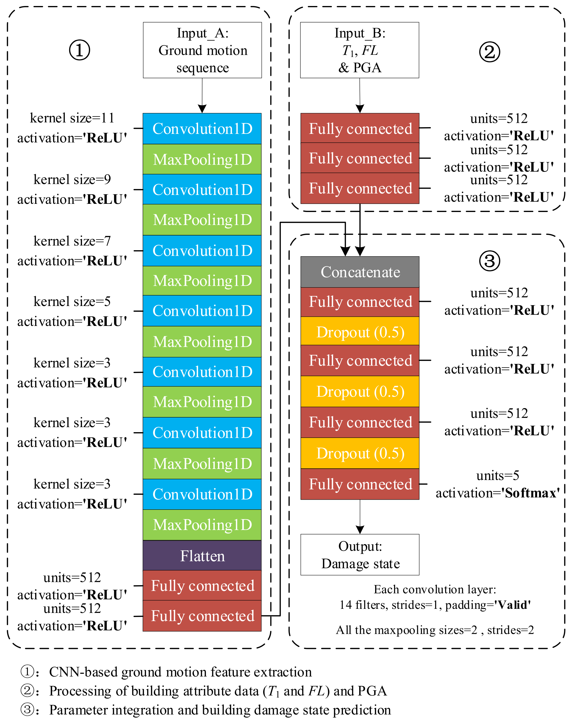
2. Methodology Framework

The model architecture is proposed based on a lot of related works [23,24] and a different number of convolutional layers, different kernel sizes, and different number nodes in fully connected layers that have been tested to yield the current model. The MI-CNN model proposed in this paper is shown in Figure 2 and can be divided into three parts:
(1)
CNN-based ground motion feature extraction
According to Zheng et al. [23], CNN can well extract the time-/frequency-domain features of ground motions. Therefore, this study adopts CNN to extract the ground motion features. Specifically, the amplitudes of all ground motion sequences were normalized to improve the performance of CNN. The normalized ground motion sequence is adopted as Input_A, and fed into seven convolutional and pooling layers, followed by two fully connected layers, through which the ground motion sequence is transformed into 512 feature parameters. The kernel sizes decrease from 11 to 3 for the seven convolutional layers. The ReLU activation function is adopted for convolutional and fully connected layers. The Softmax activation function is used for the last fully connected layer to obtain the probabilities of different damage states.
(2)
Processing of building attribute data (T1 and FL) and PGA
Consider that the ground motion sequences are normalized in Input_A and the amplitude of ground motion (PGA) together with building attribute data are Input_B. In this study, T1 and FL are utilized as building attributes to capture the nonlinear seismic performance of RC frame buildings. Other attributes can also be utilized to characterize the building properties more comprehensively. For example, the stiffness, mass, height, and designed strength for each story of a building are also very good building attributes. Nevertheless, the size of the training set is exponential to the number of building attributes considered; thus, only two building attributes (T1 and FL) are adopted in this work to avoid too many samples in the training set. Subsequently, Input_B is fed into three fully connected layers to obtain the other 512 feature parameters.
(3)
Parameter integration and damage prediction
In this part, the model concatenates all 1024 feature parameters obtained from the first and second parts, and the output is the probability of every damage state through four fully connected layers. The dropout technique is adopted to avoid overfitting and the dropout rate is set to 0.5 [25].

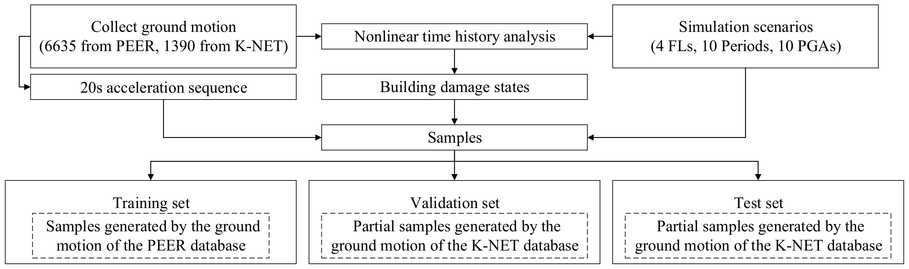
3. Sample Generation and Model Training

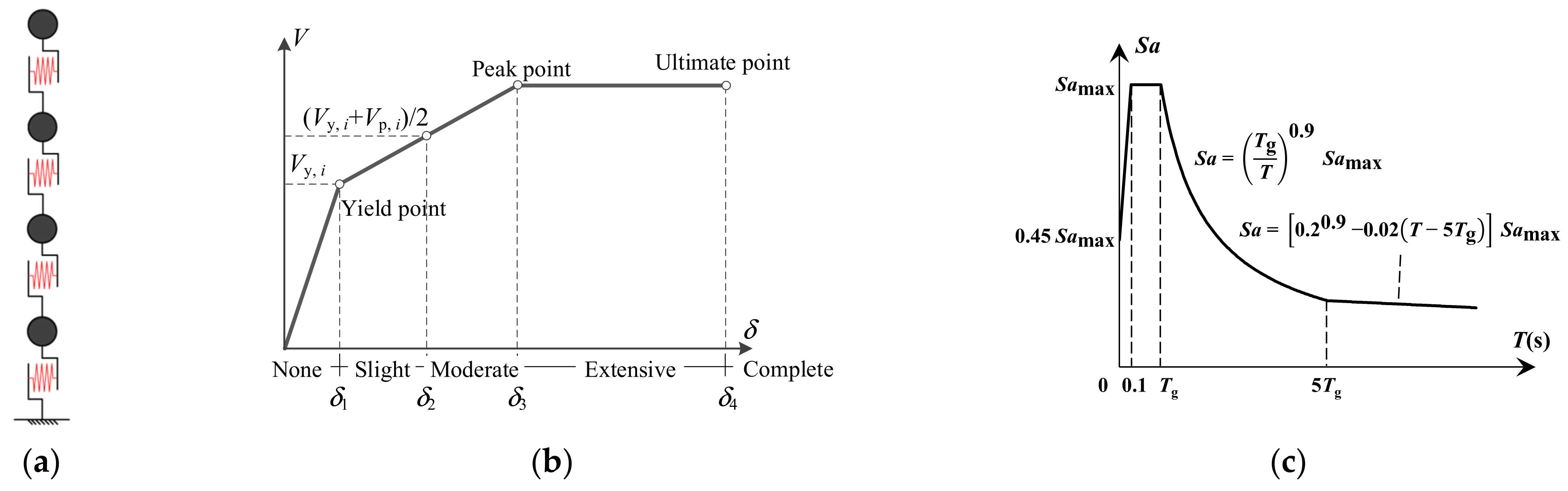
3.1. Finite Element Model

This paper focuses on the prediction of seismic damage for multi-story RC frame buildings. In order to build a training set for the MI-CNN model, 40 building models with different attribute data, including 10 fundamental periods (0.1–1 s) and 4 seismic fortification levels (levels 6, 7, 8, and 9), were set up.
The aforementioned 40 building models with different attribute data are modeled using a nonlinear multi-degree-of-freedom (MDOF) shear model, as shown in Figure 3a. This model concentrates the mass of each story in a mass point and adjacent stories are connected by shear springs, which can reflect the nonlinear seismic performance of multi-story RC frame buildings [26]. The fundamental period of a building will change when entering nonlinear state. Nevertheless, the extent of fundamental period variation is difficult to characterize, which can be influenced by many factors, such as the intensity of a ground motion and the seismic performance of a building. In this study, the fundamental period of a building in the elastic state is used to characterize the elastic property of a building. According to Chinese code [27], the elastic fundamental period is proportional to the number of stories (Equation (1) [27]), which can be used to predict the fundamental period of low- to mid-rise buildings. The damping ratio of the building model is taken as 0.05 [27].
T1 = 0.1 n
where T1 is fundamental period (unit: s) and n is the number of stories.
The story mass is determined based on the area of each story A1 and the mass per unit area m1 (Equation (2)), and the international unit is adopted for all the following equations. m1 can be estimated according to the occupancy of each story. In this study, the A1 and m1 were set to 1000 m2 and 1000 kg/m2 for all building models.
m = m 1 A 1
The stiffness of each story is assumed uniformly distributed along the height. Given the fundamental period T1 and the mass of each story, the shear stiffness k of each story can be calculated through modal analysis.
From the above procedure, the elastic parameters of a MDOF model can be obtained. Although only the fundamental period T1 is used to determine the elastic parameters, the MDOF model can consider a higher mode vibration. Moreover, considering that the elastic performance of low- to mid-rise buildings is primarily controlled by the fundamental period T1, it is also adopted as a building attribute for the following machine learning model.
The MDOF model can also capture the nonlinear performance of RC frame buildings. The tri-linear backbone curve model, as shown in Figure 3b, is adopted to simulate the seismic capacity of each story. The yield strength Vd and peak strength Vp of each story of a building can be determined by Equations (3) and (4).
V y = Ω 1 V d
V p = Ω 2 V d
Ω 2 = K 1 K 2
K 1 = 0.1671 F L 2 3.1062 F L + 16.399
K 2 = 1 ( 0.0099 n 0.0197 )
where Vd is the design shear force, which can be calculated through the equivalent static load method [22]. Ω1 and Ω2 are yield and peak overstrength ratios of RC frame, respectively, and the Ω1 is set to 1.1 [26] and Ω2 can be calculated through Equations (5)–(7). FL and n are the fortification level and the number of stories. Equations (6) and (7) were obtained through the statistical analysis of 155 pushover results of RC frames designed following the Chinese seismic design code [22]. More details on the MDOF shear model can be found in the former study of Xiong et al. [26].
Five damage states were adopted, which are none, slight, moderate, extensive, and complete damages. The damage state of each story was determined according to the damage limits shown in Figure 3b. The damage state of a building was determined according to the severest damage state among all stories. According to the Chinese code for seismic design of buildings [22], four seismic fortification levels of buildings (i.e., levels 6, 7, 8, and 9) are used in this study, which corresponds to the maximum spectral acceleration Samax of 0.04 g, 0.08 g, 0.16 g, and 0.32 g, respectively, in the design spectrum (Figure 3c) [22].
Figure 3. Building model: (a) MDOF shear model; (b) tri-linear backbone curve model; (c) design response spectrum of the Chinese code for the seismic design of buildings [22].
Applsci 11 08258 g003

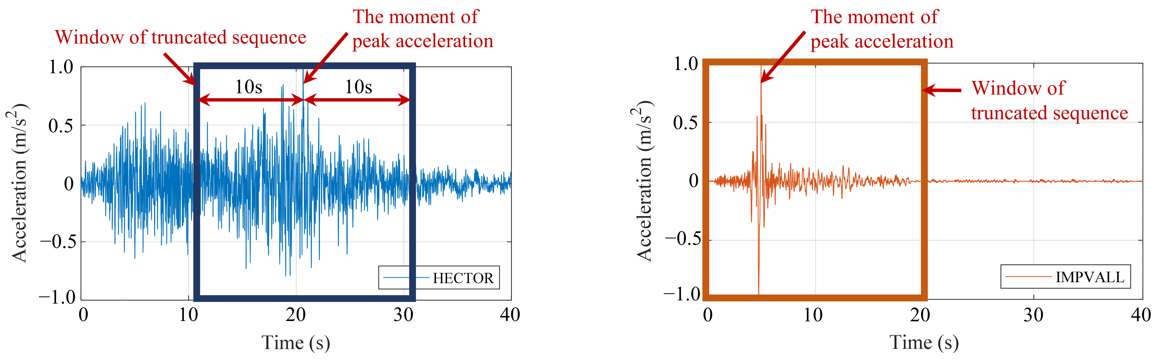
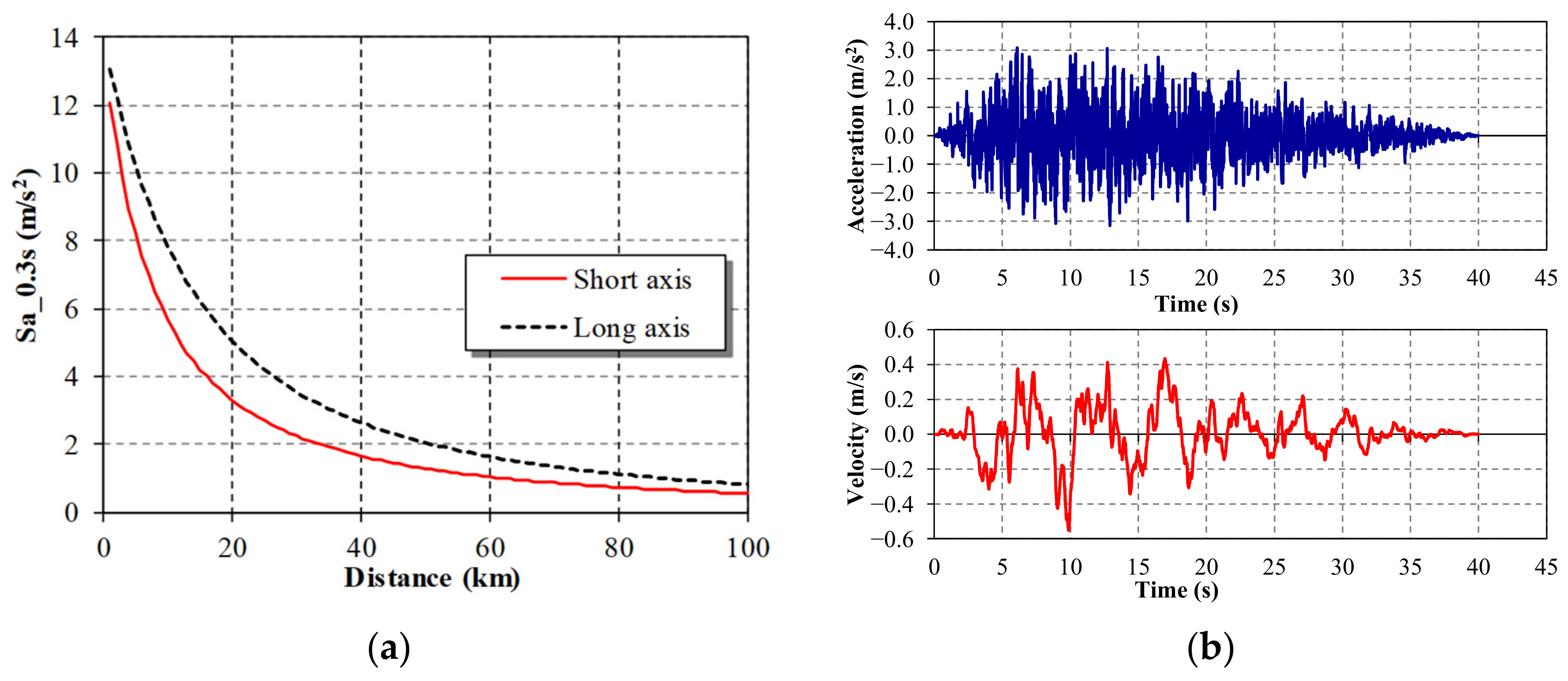
3.2. Processing of Ground Motion Sequences
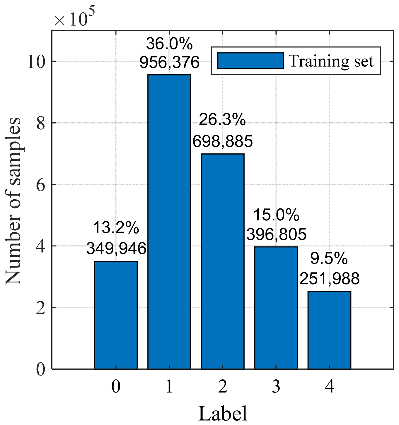
The processing flow of ground motion sequences is shown in Figure 4. Firstly, 6635 ground motion records were collected from PEER’s ground motion database [28] for generating the training set. Meanwhile, 1390 ground motion records were collected from the K-Net database [29], for generating the validation and test sets. Subsequently, each ground motion sequence was scaled to 10 different amplitudes (i.e., PGA = 1–10 m/s2), resulting in 80,250 ground motions.
The 40 building models established in Section 3.1 were analyzed using the collected ground motions through time history analysis and the damage states of all buildings were calculated. The damage states are none, slight, moderate, extensive, and complete damages, which are labeled as 0, 1, 2, 3, and 4, respectively. The labeled samples are prepared for the use of model training in the next section.
Since ground motion records were collected from different stations with different sampling rates and durations, it is necessary to down sample and truncate the ground motion records to meet the needs of the MI-CNN model. Specifically, all ground motion records were down sampled to 50 Hz, and truncated to 20 s sequences, i.e., 10 s before and after the peak acceleration point, to ensure the same data size for all ground motion sequences. If a ground motion does not have enough data before or after the peak acceleration point, the 20 s time window will be shifted backward or forward to ensure that the peak acceleration is close to the center of the truncated sequence (Figure 5). The processing of a ground motion record results in a sequence of 1000 acceleration points.
The processed ground motion sequences, PGA, the building fundamental period (T1), and the building seismic fortification level (FL) together with the calculated damage states of buildings were collected as samples for training, validating, and testing the proposed MI-CNN model. The distribution of samples in the training set is presented in Figure 6.
It is noteworthy that the samples generated from 6635 ground motion records of PEER were used as the training set, while the samples generated from 1390 ground motion records of K-Net were used as the validation and testing sets. This makes sure that the training and testing sets are generated from different earthquakes, which means the testing of the MI-CNN model is rigorous, and the testing results can demonstrate the applicability of the model in predicting building seismic damages for future earthquakes.

3.3. Model Training

In the training model, the Adam optimizer [30] was adopted for optimization, considering its high computational efficiency and low memory requirement. The learning rate was set as 0.001 and the selection of other parameters followed the default values recommended by Kingma et al. [30]. For example, β1 was set as 0.9, β2 was set as 0.999, and ε was set as 10−8, and previous research has shown that the Adam algorithm performs well with these default parameter settings [31]. The categorical cross entropy was used as the loss function, and the mathematical expression of the categorical cross entropy is as follows:
L = 1 N i = 1 N c = 0 M y i c log ( p i c )
where L is the loss value, i is the sample index, c is the class index, N is the number of samples, M is the number of labels, yic is a signum (if the actual class of the sample i is equal to c, it is 1, otherwise it is 0), and pic is the prediction probability of sample i in class c [32].
The maximum epoch was set as 500. The accuracies of training and validation were recorded at the end of each epoch. The early stopping function [33] was adopted in the training, which will stop the training early to avoid overfitting and output the best model parameters. Since the training set contains 2,654,000 samples (66,350 ground motion sequences times 40 buildings), the data set is large and it is difficult to perform the training using all samples at once. The training set was randomly divided into four batches. The training of each batch stopped when the validation accuracy no longer improved in the following 40 epochs. The weights of the epoch with the highest validation accuracy in the former batch are used as the initial weights for the next batch. The training/validation accuracies of all four batches are shown Figure 7.
Figure 7 shows that the training accuracy increases at the beginning and then stabilizes to approximately 90%. It is worth noting that the training accuracy increases relatively slow for Batch 1, where the training accuracy is less than 80% until the 10th epoch. This is because the model is learning the potential law of the training samples. Moreover, the number of epochs required to achieve above an 80% training accuracy decreases for the subsequent batches, indicating that after the first batch, the model has obtained appropriate weights applicable to the rest of the batches.
The validation accuracy of the first batch reached 77.5% at the 7th epoch; although this is the highest validation accuracy among all four batches, it is not adopted as the optimal epoch because the model has not learned from the following batches. The weights of the 7th epoch in Batch 1 were used as the initial weights of Batch 2, and the highest validation accuracy of Batch 2 was attained at the 32nd epoch. The training and validation accuracies are 86.6% and 77.1%, respectively. The weights of the 32nd epoch of Batch 2 were used as the initial weights of the following batches. The highest validation accuracies were obtained at the first epoch of Batch 3 and Batch 4, indicating that the weights of 32nd epoch of Batch 2 can reasonably capture the properties of the following batches. Therefore, the weights of the 32nd epoch of Batch 2 were used as the optimal weights of the proposed model.

4. Discussion of Prediction Results

4.1. Prediction Performance of Different Scenarios

The overall confusion matrix of the test set is shown in Figure 8. The overall test accuracy is 79.7%, and the prediction accuracies of all damage states are around 80%. Meanwhile, more than 90% of the predicted damage states are within one level difference to the actual damage states. Note that ground motions in the training set come from pre-2003 earthquakes in the PEER database, while ground motions in the validation and test sets come from post-2003 earthquakes in the K-Net database. This arrangement ensures that the ground motions adopted to test the accuracy of the model are completely different from those used to train the model. Therefore, the test accuracy of 79.7% indicates that the proposed method can reasonably predict seismic damage of building even for earthquakes that do not exist in the training set.
Moreover, the computation efficiency of the MI-CNN model is significantly better than the nonlinear time history analysis of the MDOF shear model. For example, the computation time of 278,000 samples in the test set is 31.38 s for the MI-CNN model, which is 340 times faster than the nonlinear time history analyses of MDOF shear models (170 min) on a laptop platform (AMD Ryzen 5 3600, RAM 32 G, GPU GTX1660S).
To further demonstrate the prediction performance of the MI-CNN model, samples in the test set with different PGAs, building fundamental periods, and fortification levels are discussed separately.
The sensitivity analysis of results on fundamental period is shown in Figure 9a, and the prediction accuracy of most samples is around 80%. Nevertheless, the prediction accuracy for Labels 3 and 4 with PGA of 1 m/s2 is missing, and this is because the PGA of 1 m/s2 is relatively small, and no sample reaches the severe and complete damage states when PGA is 1 m/s2. Moreover, the prediction accuracies for Labels 3 and 4 in the PGA range of 1–3 m/s2 are still relatively poor; to further investigate the reason for this, the distribution of the training set together with the prediction accuracies for samples with PGA of 1–3 m/s2 are illustrated in Figure 9b. As is evident in Figure 9b, the prediction accuracies are relatively low for Labels 3 and 4 (64.3% and 59.1%). This is because the proportion of training set samples in Labels 3 and 4 are very small (2.3% and 0.3%), which can jeopardize the prediction accuracy for this scenario. It is worth noting that this skewed distribution of the training set in the PGA range of 1–3 m/s2 is not a mistake, this is because there are some very unique ground motions with a very strong destructive power to mid-rise buildings, even with a very small PGA. The authors think that this is a limitation of the proposed model, and further studies are required to consider this exceptional scenario.
The confusion matrices for cases with different PGAs are presented in Figure 10. The prediction accuracies of all PGA bands are above 77%. It is worth noting that, according to Figure 1a, when the ground motion intensity measure is large, the building seismic response can be very dispersed. Nevertheless, as shown in Figure 10d, the prediction accuracy for buildings with a large PGA can still yield good accuracy (77.5%), which indicates that the MI-CNN model can effectively predict the seismic response of buildings in very strong nonlinearity.
The sensitivity analysis on the fundamental period is demonstrated in Figure 11a. The results indicate that the prediction accuracy of most samples is also around 80%, while the prediction accuracies for Labels 2, 3, and 4 are relatively poor, especially in the T1 range of 0.8–1.0 s. Therefore, the distribution of the training set and prediction accuracies for samples with a T1 range of 0.8–1.0 s are further illustrated in Figure 11b. In Figure 11b, the prediction accuracies of Labels 2, 3, and 4 are approximately 60%, while the prediction accuracies with one level differences are all above 90%. One possible reason for these relatively poor prediction accuracies is the relatively small proportion of samples in these classes of the training set. This is also a limitation of the proposed model, and further investigation can be conducted to improve the prediction accuracy through methods such as active learning [16].
Figure 12 shows the confusion matrices for buildings with different fundamental periods. The results show that the model can achieve the prediction accuracy of approximately 80% for buildings with different fundamental periods.
Figure 13 shows the confusion matrices for buildings with different fortification levels, which also exhibit approximately 80% accuracy for all scenarios. The above results show that the prediction accuracies of most classes are around 80%, and more than 90% of the predicted damage states are within one level difference to the actual damage states. Nevertheless, the prediction accuracies of some individual classes are below 70%. Note that the number of samples is small for classes with below 70% accuracy, which indicates that the proposed method can reasonably predict the seismic damages for most cases, and further studies are needed to improve the prediction accuracies of some individual classes.

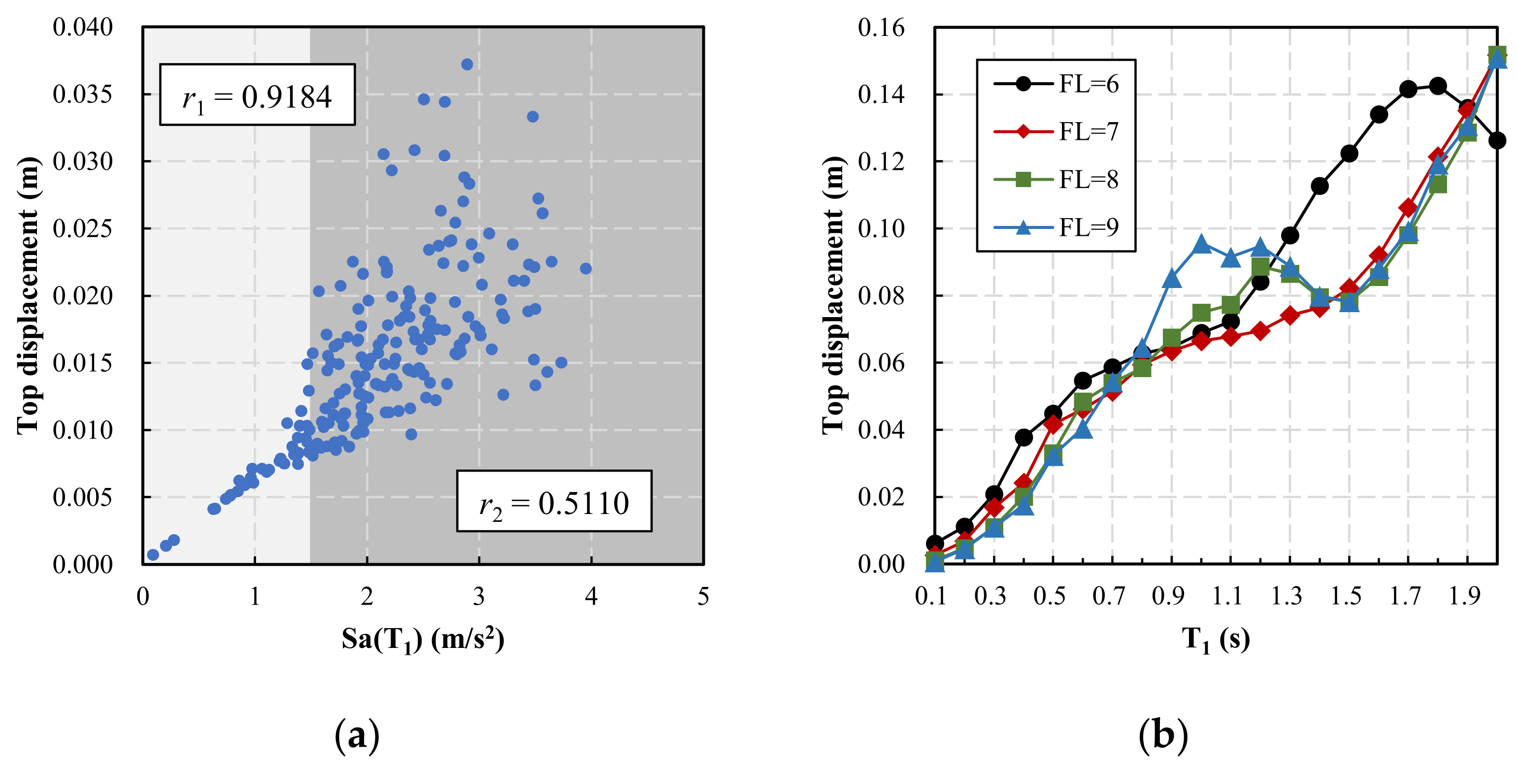
4.2. Comparison with the Method Based on Ground Motion Intensity Measures

Ground motion intensity measures are often adopted to reflect the destructive power of earthquakes in machine learning-based seismic damage assessment methods. For example, Mangalathu et al. [16] used Sa(T1) as the ground motion intensity measure and combined it with structural parameters to predict the seismic damage of bridges. Therefore, in this section, a comparative analysis was conducted to investigate the performance of the MI-CNN model (adopting the ground motion sequence as the input) and the method based on ground motion intensity measures.
For the method based on ground motion intensity measures, the PGA, peak ground velocity (PGV), maximum spectral acceleration (Samax), and spectral acceleration of fundamental period Sa(T1) were calculated for the collected ground motions. The calculated four ground motion intensity measures were combined with the building attribute data (building fundamental period and fortification level) to form each sample for model training. The division of the training, validation, and test sets is consistent with the previous section.
As for the selection of machine learning models for the comparative analysis, the LightGBM and XGBoost models have been widely used in classification problems with multiple feature inputs [34,35]. These two models have the advantages of good training efficiency, low memory consumption, and high accuracy compared to other machine learning models. Therefore, the LightGBM and XGBoost models were adopted as the machine learning model for the comparative analysis. During the training process, the Multiclass_Logloss multi-category logarithmic loss function was adopted, and the maximum epoch was set to 50. The early stopping function was also used in this section.
The confusion matrices for the method based on ground motion intensity measures are shown in Figure 14. The prediction accuracies of the test set using the LightGBM and XGBoost models are 73.7% and 67.4%, respectively. These accuracies are lower than those of the MI-CNN (prediction accuracy = 79.7% in Figure 8). The above results show that the proposed MI-CNN model can better predict the seismic damage of buildings compared to the method based on ground motion intensity measures.

5. Case Study of an Urban Area

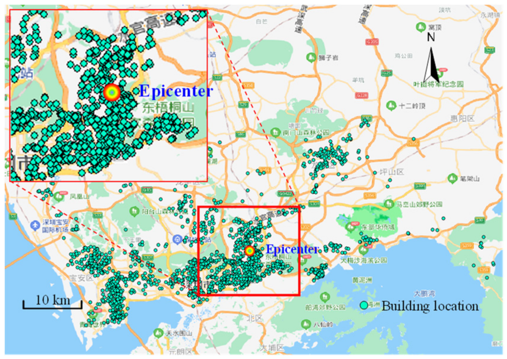
5.1. Information of the Area

To further demonstrate the proposed method, a case study of Shenzhen city is presented in this section. Studied buildings are RC frame buildings with no more than 10 stories. The distribution of studied buildings is shown in Figure 15. These building data were obtained from an online apartment rental company [36]. Note that the primary purpose of the case study is not to obtain the accurate seismic damage of Shenzhen city, but to demonstrate the effectiveness of the proposed method. If more reliable data become available in the future, a more accurate simulation can be performed using the methods presented in this work.

5.2. Earthquake Data

Based on the seismic hazard analysis of Xu et al. [37], two earthquake scenarios of M6.5 and M7.5 were selected. The epicenter is located in the Jiuweiling fault with a fault strike of 46 degrees. Based on the Chinese response spectrum attenuation function [38] and the site amplification factor [39], the seismic response spectrum data of the whole area were obtained and the ground motion of the whole area was generated by the artificial ground motion generation program SIMQKE [40]. The attenuation functions and a typical ground motion time history are shown in Figure 16. Figure 17 shows the location of the epicenter and the distribution of the response spectrum parameter Sa(0.3s) across the region for the two earthquake scenarios.

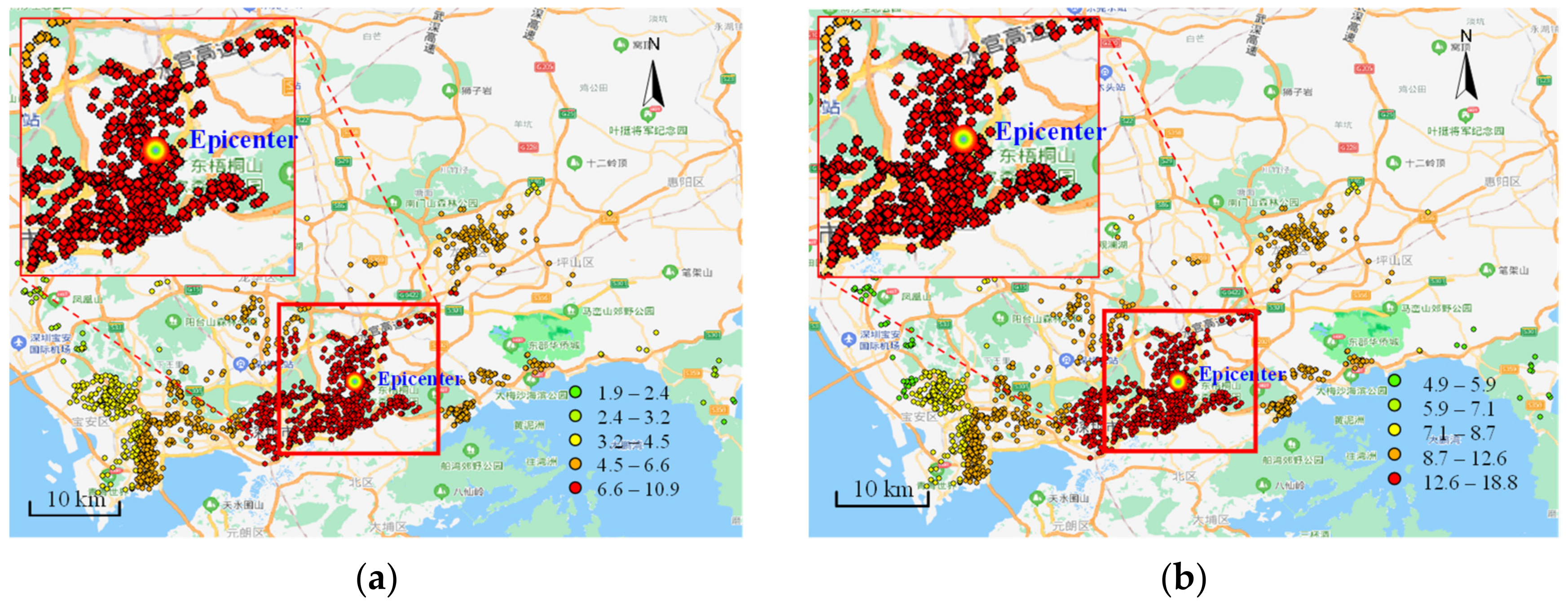
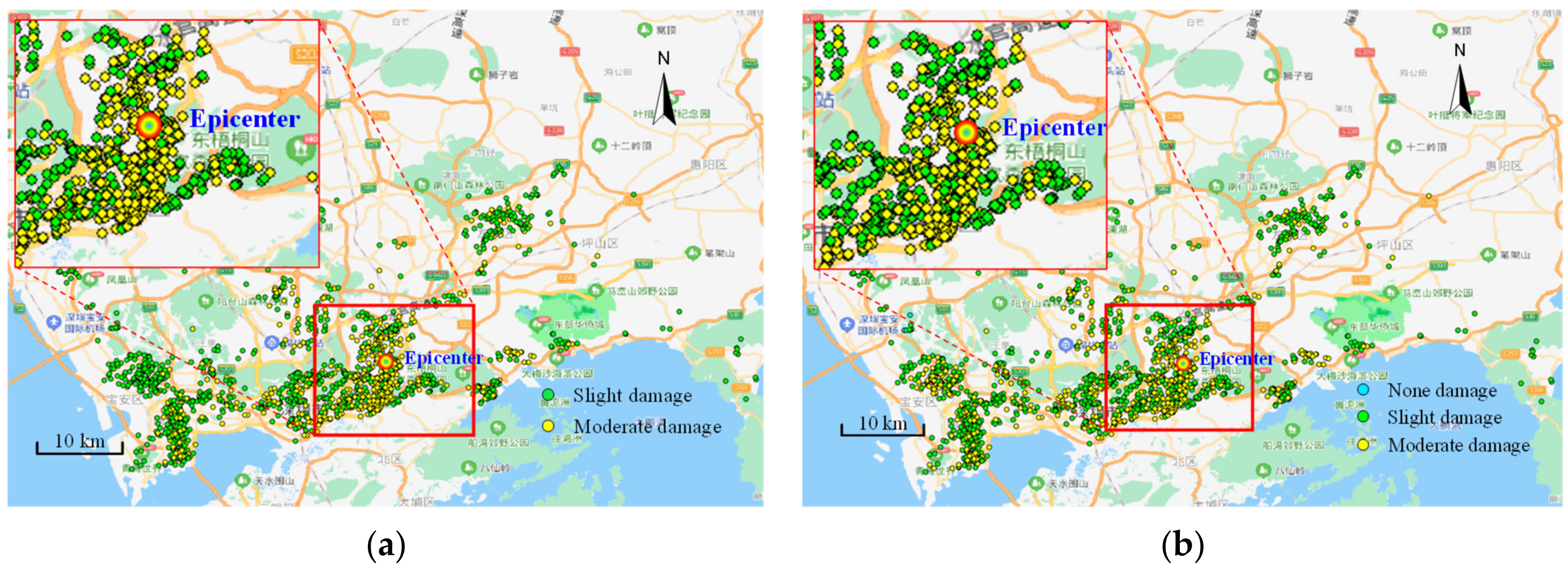
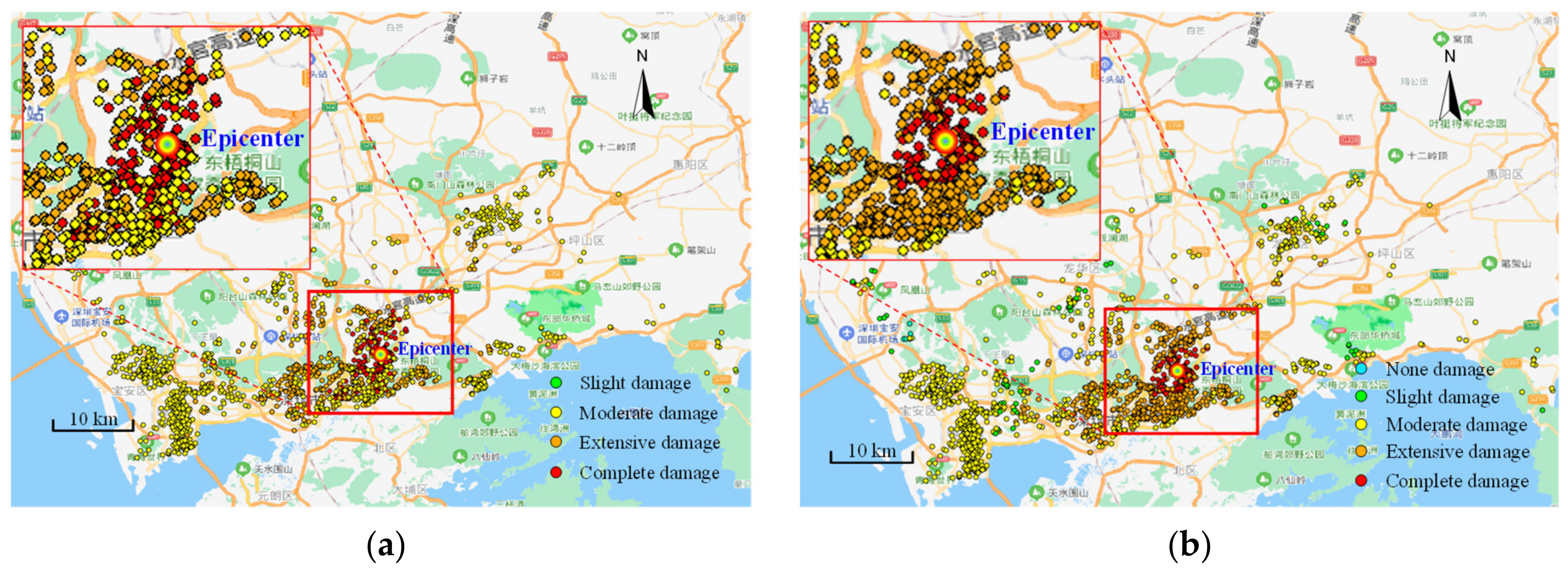
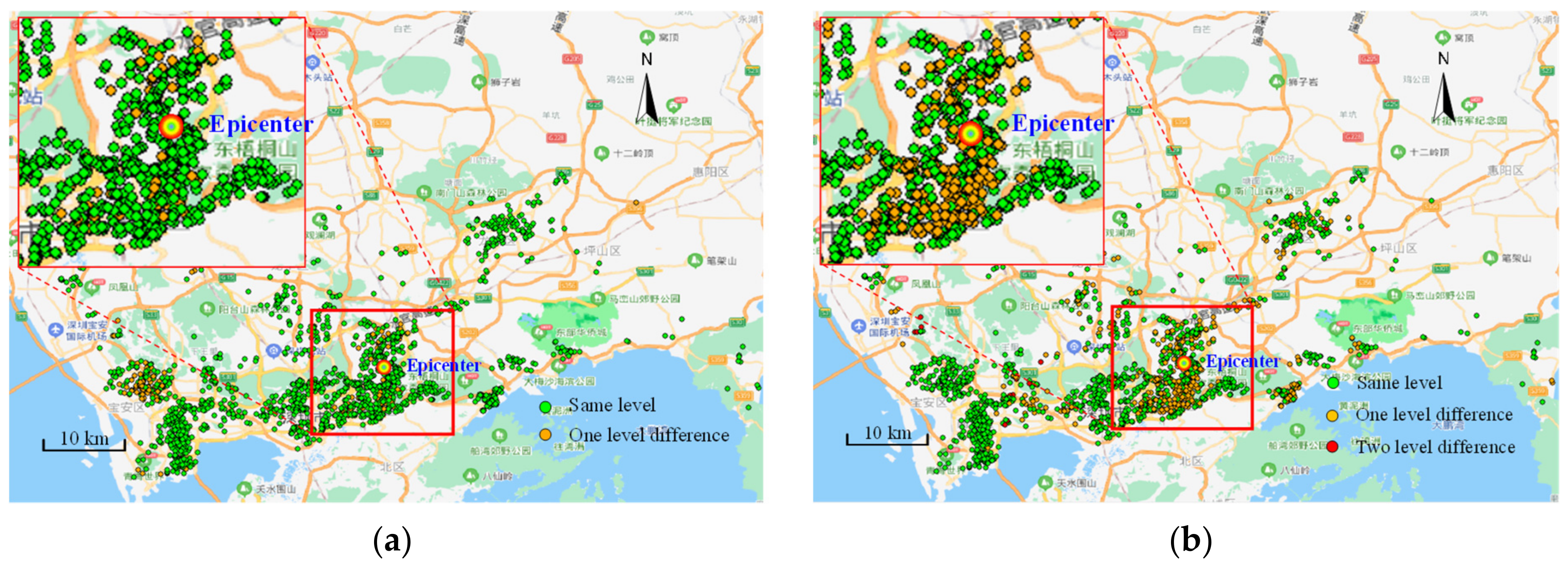
5.3. Simulation Results

Time history analyses were performed for all buildings. First, the mass, stiffness, and strength parameters of MDOF models were determined according the procedure presented in Section 3.1. Subsequently, time history analyses were performed for all buildings and the damage states of were determined according to the limit state as shown in Figure 3. The results of the time history analysis using MDOF shear model and the MI-CNN model for the M6.5 earthquake scenario are shown in Figure 18. The results of the time history analysis were adopted as the benchmark results to demonstrate the accuracy of the proposed MI-CNN model. The results show that the MI-CNN prediction agrees well with the time history analysis results. Most of the buildings exhibit slight to moderate damages, and buildings near the epicenter exhibit more severe damages.
The prediction results for the M7.5 earthquake scenario are shown in Figure 19. The results also show a good agreement between the MI-CNN results and the time history analysis results.
According to the results in Figure 18 and Figure 19, the prediction error of the MI-CNN model compared to the time history benchmark model are presented in Figure 20. For the M6.5 earthquake scenario, only 151 out of 1760 buildings experienced a one-level error, while the rest of the 1609 buildings are in the same damage states as in the benchmark results; for the M7.5 earthquake scenario, 15 buildings experienced a two-level error and 420 buildings experienced a one-level error, while the rest of the 1325 buildings have the same damage states as in the time history results. The above simulation results show that the proposed MI-CNN prediction results have a good prediction accuracy.

6. Conclusions

A multiple-input CNN (MI-CNN) model is proposed in this study to consider the time-/frequency-domain characteristics of ground motions and attribute data of buildings. The proposed model can achieve a good prediction accuracy and significantly better computational efficiency compared to nonlinear time history analysis of the MDOF shear model. Some detailed conclusions can be drawn as follows:
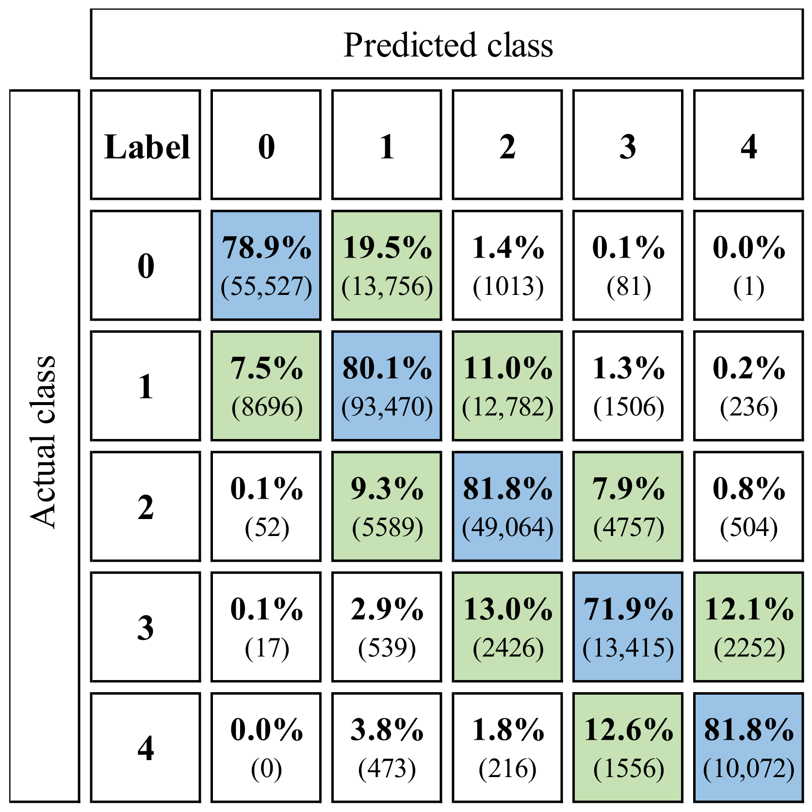
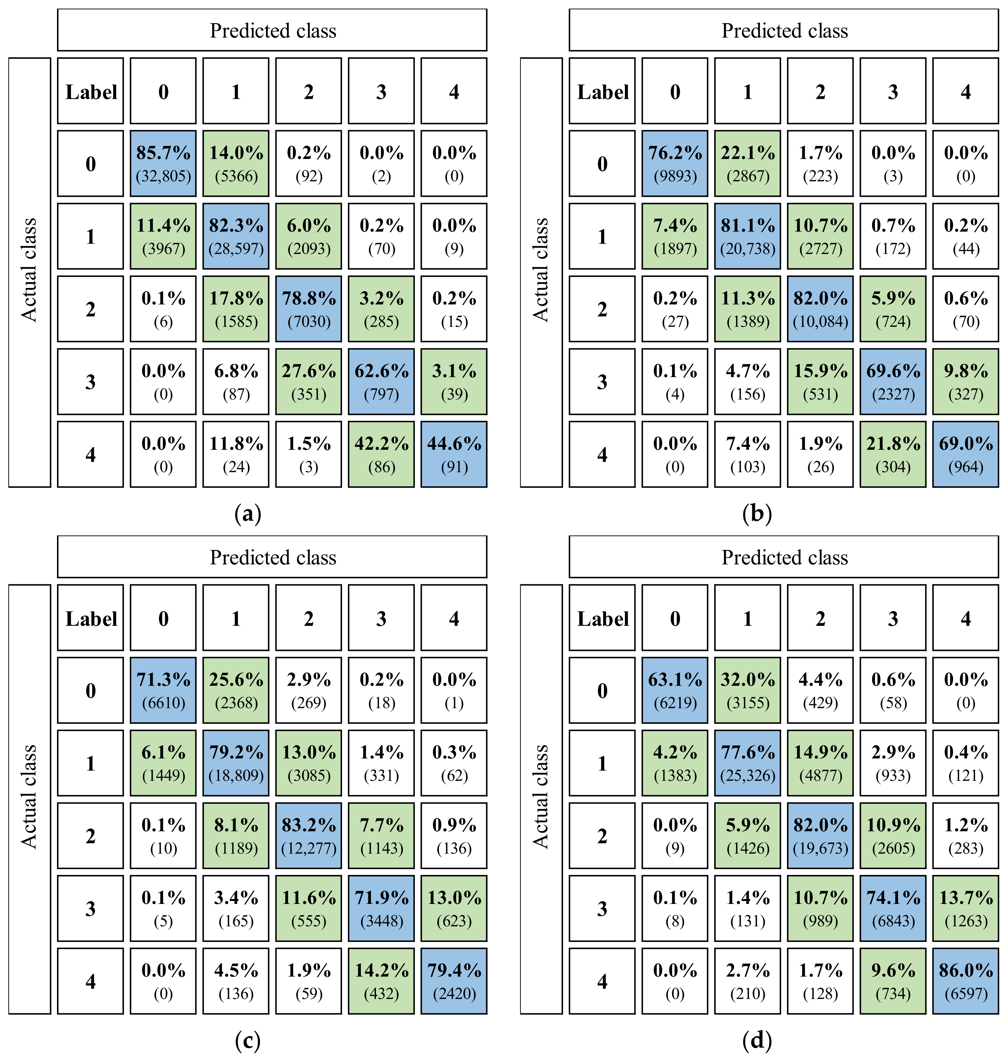
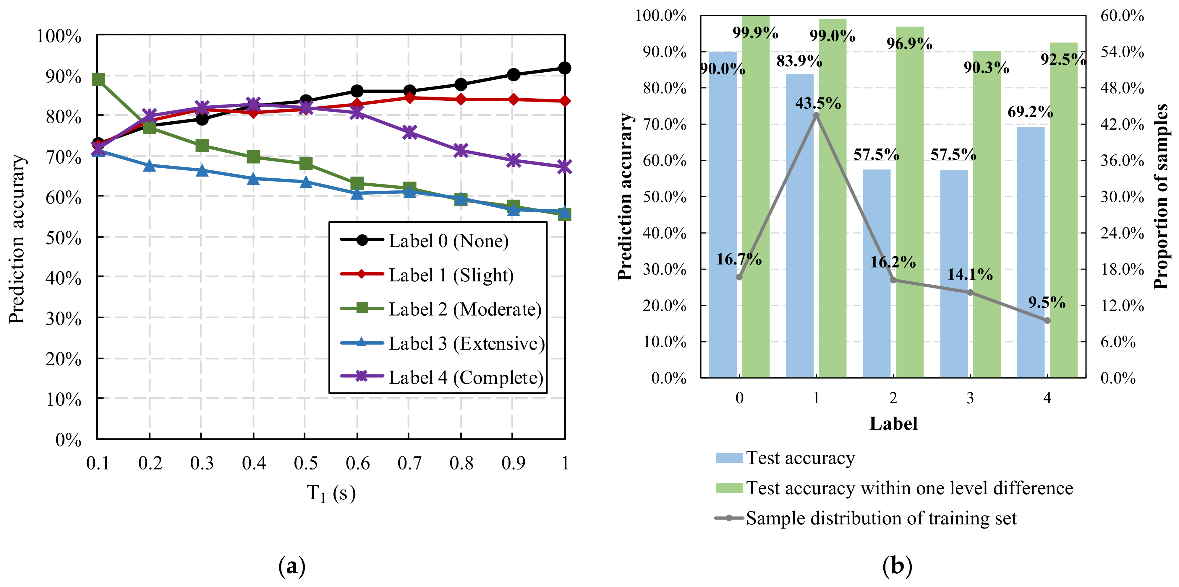
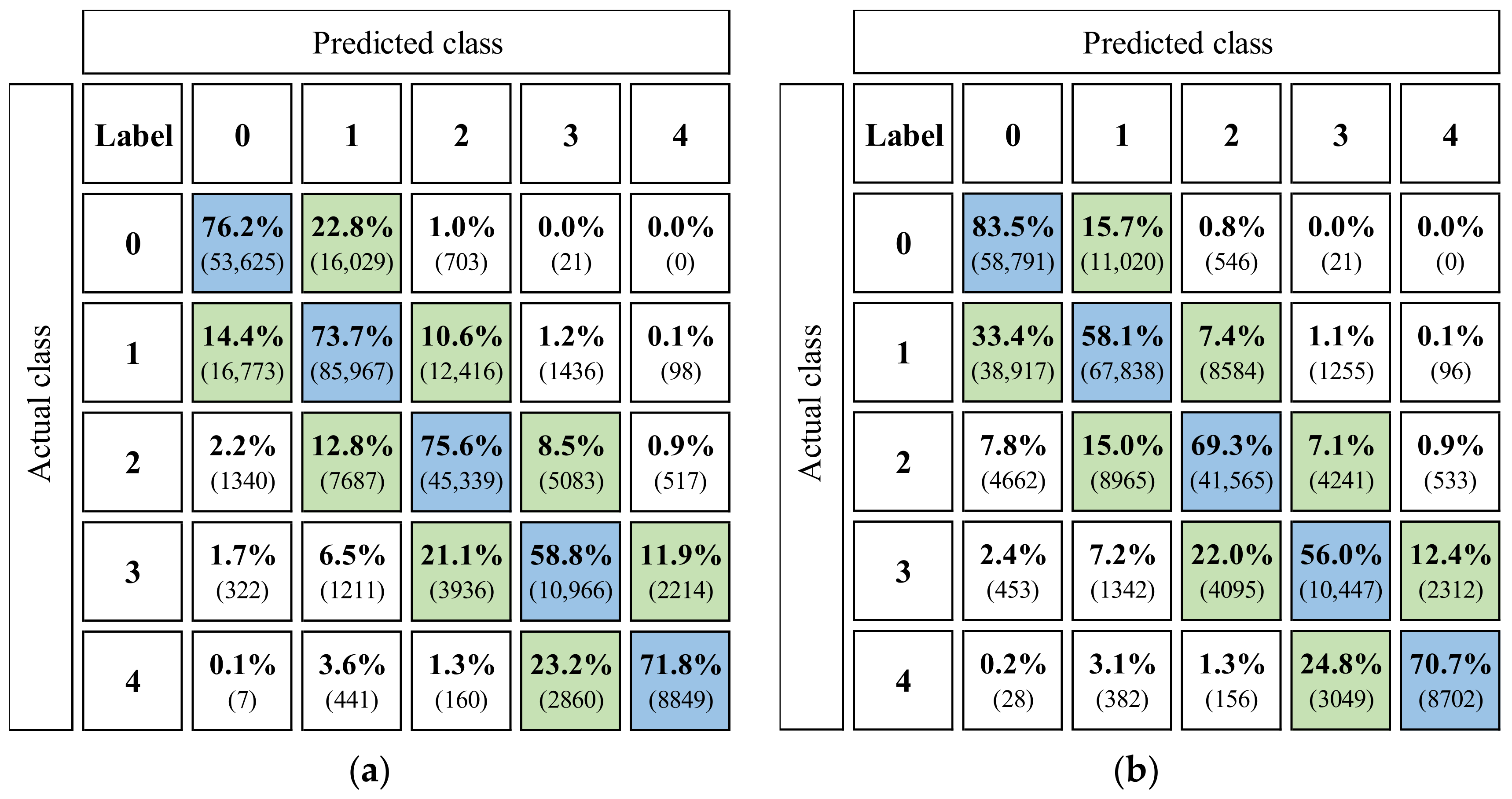
  • The proposed MI-CNN model can achieve the overall prediction accuracy of 79.7% for the test set, and more than 90% of the predicted damage states are within one level of difference to the actual damage states.
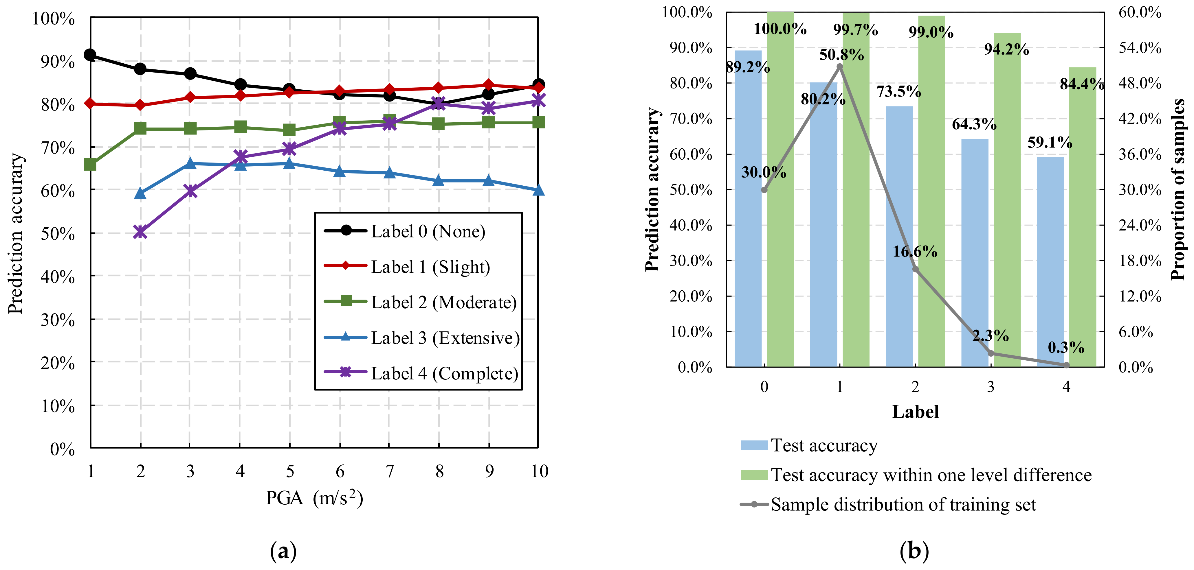
  • The prediction accuracies for cases with different PGAs, building fundamental periods, and fortification levels are also around 80%, which shows good prediction performance of the model in different simulation scenarios.
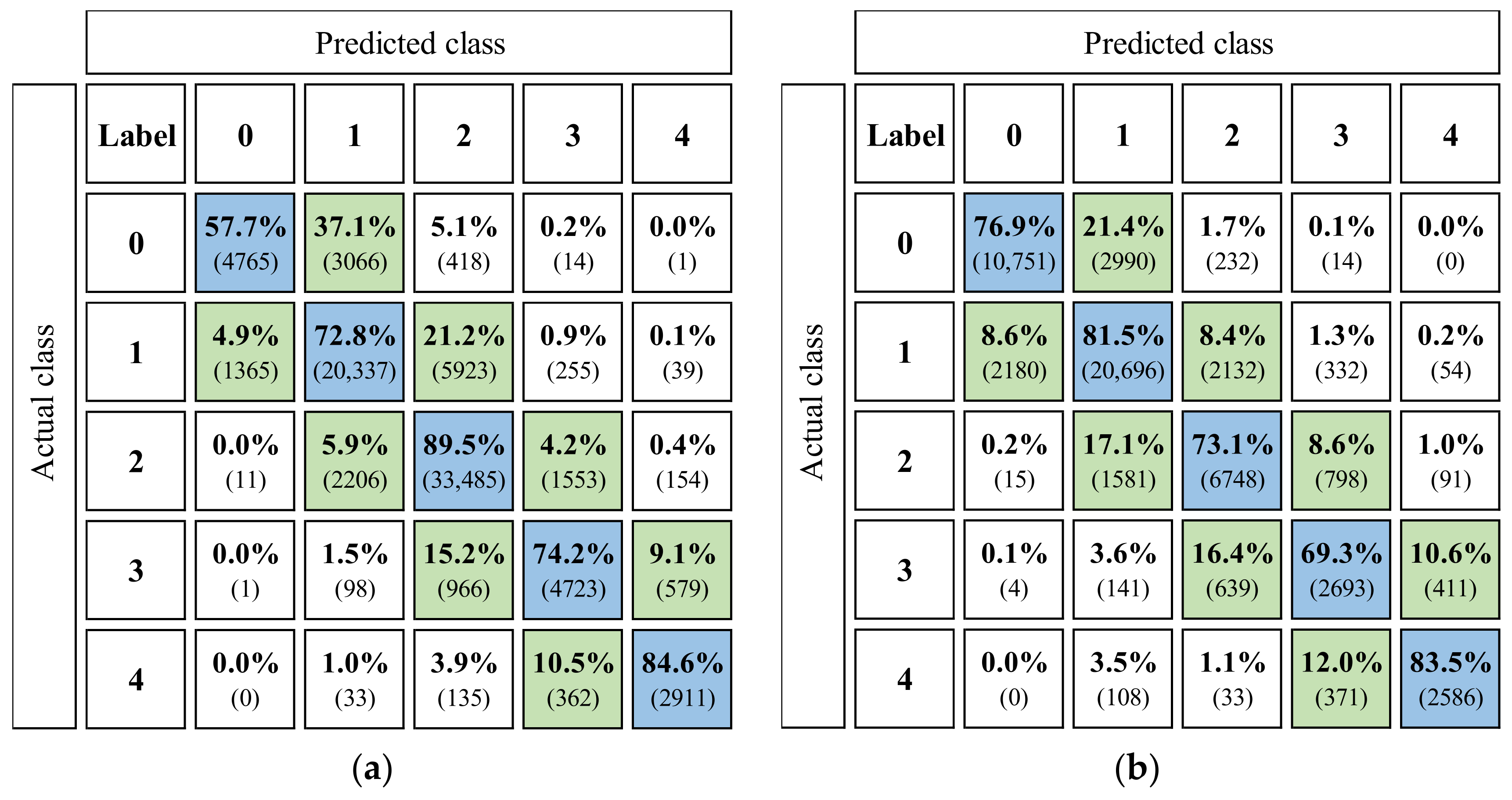
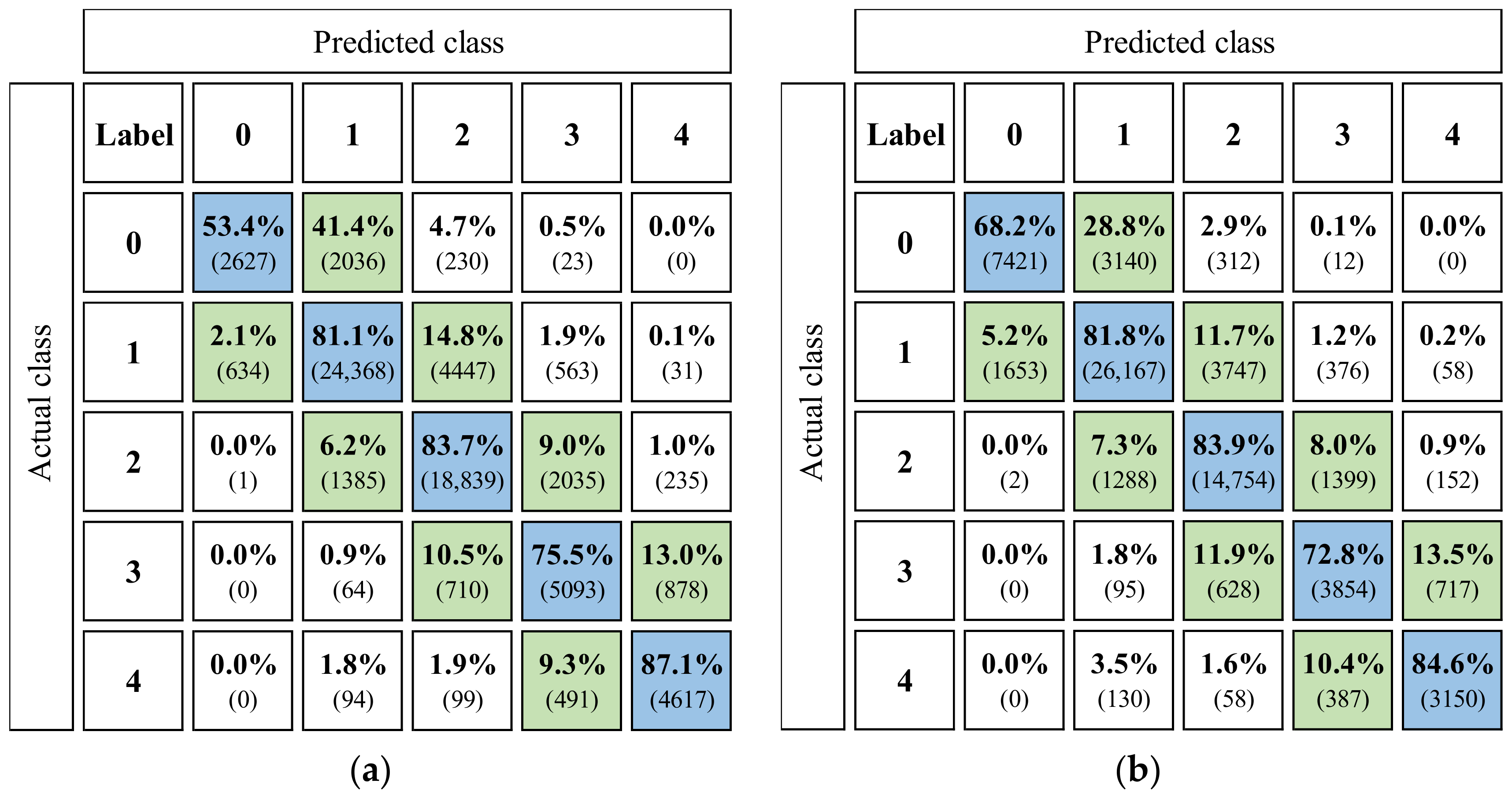
  • The prediction performance of the proposed model is compared with methods using ground motion intensity measures as the earthquake input. The prediction accuracy of the proposed MI-CNN model is 79.7%, which outperforms the simulation using PGA, PGV, Samax, and Sa(T1) as earthquake inputs (73.7%).
  • The computation efficiency of the proposed model is significantly better than nonlinear time history analysis of MDOF shear model. The speedup ratio is 340 on a laptop platform.
  • The prediction accuracy for some individual classes is relatively low (less than 70%), which is caused by some very unique ground motions and a relatively small number of samples in the corresponding classes. This is a limitation of the proposed method, and further investigation can be conducted to improve the prediction accuracy through methods such as active learning.
The proposed MI-CNN model can be a useful tool for the fast seismic damage assessment of regional buildings. The outcomes of this work are expected to assist in post-disaster emergency response and rapid disaster relief.

Author Contributions

Conceptualization, C.X.; Data curation, J.Z., R.Z. and C.C.; Funding acquisition, L.X., Y.L. and C.X.; Investigation, C.X., J.Z. and C.C.; Methodology, C.X. and J.Z.; Project administration, L.X. and C.X.; Resources, L.X., C.X. and Y.L.; Software, C.X., R.Z. and J.Z.; Supervision, L.X. and C.X.; Writing—original draft, C.X., J.Z. and C.C.; Writing—review and editing, C.X., J.Z. and C.C. All authors have read and agreed to the published version of the manuscript.

Funding

This research was funded by the National Key Research and Development Program (Grant No. 2019YFC1511003), the Intellectual Innovation Program of Shenzhen Science and Technology Innovation Committee (Grant No. JCYJ20180305123919731), and the National Natural Science Foundation of China (Grant No. 51708361).

Conflicts of Interest

The authors declare no conflict of interest.

References

  1. Bilham, R. Lessons from the Haiti earthquake. Nature 2010, 463, 878–879. [Google Scholar] [CrossRef]
  2. Ye, L.; Lu, X.; Li, Y. Design objectives and collapse prevention for building structures in mega-earthquake. Earthq. Eng. Eng. Vib. 2010, 9, 189–199. [Google Scholar] [CrossRef]
  3. Applied Technology Council (ATC). Earthquake Damage Evaluation Data for California; ATC-13 Report; Applied Technology Council: Redwood, CA, USA, 1985. [Google Scholar]
  4. Whitman, R.V.; Reed, J.W.; Hong, S.T. Earthquake damage probability matrices. In Proceedings of the Fifth World Conference on Earthquake Engineering, Rome, Italy, 25–29 June 1973; pp. 2531–2540. [Google Scholar]
  5. Federal Emergency Management Agency (FEMA). Earthquake Loss Estimation Methodology (HAZUS 97); Federal Emergency Management Agency: Washington, DC, USA, 1997.
  6. Lai, T.W.; Liu, P.M.; Kao, M.S.S. Demonstration project of earthquake hazard for Chia-i City of Taiwan. In Proceedings of the 13th World Conference on Earthquake Engineering, Vancouver, BC, Canada, 1–6 August 2004. [Google Scholar]
  7. Remo, J.W.; Pinter, N. Hazus-MH earthquake modeling in the central USA. Nat. Hazards 2012, 63, 1055–1081. [Google Scholar] [CrossRef]
  8. Levi, T.; Bausch, D.; Katz, O.; Rozelle, J.; Salamon, A. Insights from Hazus loss estimations in Israel for Dead Sea transform earthquakes. Nat. Hazards 2015, 75, 365–388. [Google Scholar] [CrossRef]
  9. Hori, M. Introduction to Computational Earthquake Engineering; Imperial College Press: London, UK, 2006. [Google Scholar]
  10. Xiong, C.; Lu, X.; Huang, J.; Guan, H. Multi-LOD seismic-damage simulation of urban buildings and case study in Beijing CBD. Bull. Earthq. Eng. 2019, 17, 2037–2057. [Google Scholar] [CrossRef]
  11. Xiong, C.; Huang, J.; Lu, X. Framework for city-scale building seismic resilience simulation and repair scheduling with labor constraints driven by time–history analysis. Comput. Aided Civ. Infrastruct. Eng. 2020, 35, 322–341. [Google Scholar] [CrossRef]
  12. Xiong, C.; Lu, X.; Guan, H.; Xu, Z. A nonlinear computational model for regional seismic simulation of tall buildings. Bull. Earthq. Eng. 2016, 14, 1047–1069. [Google Scholar] [CrossRef]
  13. Ruggieri, S.; Porco, F.; Uva, G.; Vamvatsikos, D. Two frugal options to assess class fragility and seismic safety for low-rise reinforced concrete school buildings in Southern Italy. Bull. Earthq. Eng. 2021, 19, 1415–1439. [Google Scholar] [CrossRef]
  14. Kwag, S.; Ryu, Y.; Ju, B.S. Efficient seismic fragility analysis for large-scale piping system utilizing Bayesian approach. Appl. Sci. 2020, 10, 1515. [Google Scholar] [CrossRef] [Green Version]
  15. Battaglia, L.; Ferreira, T.M.; Lourenço, P.B. Seismic fragility assessment of masonry building aggregates: A case study in the old city Centre of Seixal, Portugal. Earthq. Eng. Struct. Dyn. 2021, 50, 1358–1377. [Google Scholar] [CrossRef]
  16. Mangalathu, S.; Jeon, J.S. Regional seismic risk assessment of infrastructure systems through machine learning: Active learning approach. J. Struct. Eng. 2020, 146, 04020269. [Google Scholar] [CrossRef]
  17. Xu, Y.; Lu, X.; Tian, Y.; Huang, Y. Real-time seismic damage prediction and comparison of various ground motion intensity measures based on machine learning. J. Earthq. Eng. 2020, 1–21. [Google Scholar] [CrossRef]
  18. Xu, Y.; Lu, X.; Cetiner, B.; Taciroglu, E. Real-time regional seismic damage assessment framework based on long short-term memory neural network. Comput. Aided Civ. Infrastruct. Eng. 2021, 36, 504–521. [Google Scholar] [CrossRef]
  19. Xiong, C.; Li, Q.; Lu, X. Automated regional seismic damage assessment of buildings using an unmanned aerial vehicle and a convolutional neural network. Autom. Constr. 2020, 109, 102994. [Google Scholar] [CrossRef]
  20. Hamdia, K.M.; Arafa, M.; Alqedra, M. Structural damage assessment criteria for reinforced concrete buildings by using a Fuzzy Analytic Hierarchy process. Undergr. Space 2018, 3, 243–249. [Google Scholar] [CrossRef]
  21. Lu, X.; Cheng, Q.; Tian, Y.; Huang, Y. Regional ground-motion simulation using recorded ground motions. Bull. Seismol. Soc. Am. 2021, 111, 825–838. [Google Scholar] [CrossRef]
  22. Ministry of Housing and Urban-Rural Development of the People’s Republic of China (MOHURD). Seismic Design Code for Buildings; GB50011-2010; China Architecture & Building Press: Beijing, China, 2016.
  23. Zheng, R.; Xiong, C.; Deng, X.; Li, Q.; Li, Y. Assessment of earthquake destructive power to structures based on machine learning methods. Appl. Sci. 2020, 10, 6210. [Google Scholar] [CrossRef]
  24. Hamdia, K.M.; Zhuang, X.; Rabczuk, T. An efficient optimization approach for designing machine learning models based on genetic algorithm. Neural Comput. Appl. 2021, 33, 1923–1933. [Google Scholar] [CrossRef]
  25. Gao, Y.; Mosalam, K.M. Deep transfer learning for image-based structural damage recognition. Comput. Aided Civ. Infrastruct. Eng. 2018, 33, 748–768. [Google Scholar] [CrossRef]
  26. Xiong, C.; Lu, X.; Lin, X.; Xu, Z.; Ye, L. Parameter determination and damage assessment for THA-based regional seismic damage prediction of multi-story buildings. J. Earthq. Eng. 2017, 21, 461–485. [Google Scholar] [CrossRef]
  27. Ministry of Housing and Urban-Rural Development of the People’s Republic of China (MOHURD). Load Code for Building Structures; GB50009-2012; China Architecture & Building Press: Beijing, China, 2012.
  28. PEER Center. PEER ground motion database. In PEER NGA-West2 Database 2013/03; Pacific Earthquake Engineering Research Center Headquarters at the University of California: Berkeley, CA, USA, 2013. [Google Scholar]
  29. K-Net. Strong-Motion Seismograph Network (K-Net, Kik-Net). 2021. Available online: https://www.kyoshin.bosai.go.jp/kyoshin/ (accessed on 4 September 2021).
  30. Kingma, D.P.; Ba, J. Adam: A Method for Stochastic Optimization. 2014. Available online: https://arxiv.org/abs/1412.6980 (accessed on 4 September 2021).
  31. Ruder, S. An Overview of Gradient Descent Optimization Algorithms. Available online: https://arxiv.org/abs/1609.04747 (accessed on 4 September 2021).
  32. Ho, Y.; Wookey, S. The real-world-weight cross-entropy loss function: Modeling the costs of mislabeling. IEEE Access 2019, 8, 4806–4813. [Google Scholar] [CrossRef]
  33. Yao, Y.; Rosasco, L.; Caponnetto, A. On early stopping in gradient descent learning. Constr. Approx. 2007, 26, 289–315. [Google Scholar] [CrossRef]
  34. Ke, G.; Meng, Q.; Finley, T.; Wang, T.; Chen, W.; Ma, W.; Ma, W.; Ye, Q.; Liu, T.-Y. Lightgbm: A highly efficient gradient boosting decision tree. Adv. Neural Inf. Process. Syst. 2017, 30, 3146–3154. [Google Scholar]
  35. Chen, T.; Guestrin, C. Xgboost: A scalable tree boosting system. In Proceedings of the 22nd ACM Sigkdd International Conference on Knowledge Discovery and Data Mining, San Francisco, CA, USA, 13–17 August 2016; pp. 785–794. [Google Scholar]
  36. Alibaba Cloud Computing (Beijing) Co., Ltd. SFUN. Available online: https://www1.fang.com/ (accessed on 4 September 2021).
  37. Xu, J.; Yu, C.; Tang, D.; Zhang, G.; Xiao, B.; Jiang, P.; Chen, P. Active fault exploration and seismic hazard assessment in Shenzhen city. Urban Geotech. Investig. Surv. 2012, 1, 161–166. (In Chinese) [Google Scholar]
  38. Yu, Y. Study on Attenuation Relationships of Long Period Ground Motions. Ph.D. Thesis, Institute of Geophysics, China Earthquake Administration, Beijing, China, 2002. (In Chinese). [Google Scholar]
  39. Lu, H.; Zhao, F. Site coefficients suitable to China site category. Acta. Seismol. Sin. 2007, 20, 71–79. [Google Scholar] [CrossRef]
  40. Gasparini, D.; Vanmarcke, E.H. SIMQKE, A Program for Artificial Motion Generation; Department of Civil Engineering, Massachusetts Institute of Technology: Cambridge, MA, USA, 1976. [Google Scholar]
Figure 1. Correlation between the ground motion intensity measure, building attribute, and building top displacement: (a) relationship between ground motion intensity measure Sa(T1) and building top displacement; (b) relationship between building attributes and building top displacement.
Applsci 11 08258 g001
Figure 2. Schematic diagram of the MI-CNN model.
Applsci 11 08258 g002
Figure 4. Processing flow of ground motion sequences.
Applsci 11 08258 g004
Figure 5. Schematic diagram of ground motion truncation.
Applsci 11 08258 g005
Figure 6. Distribution of damage states in the training set.
Applsci 11 08258 g006
Figure 7. Training and validation accuracies of the four batches: (a) Batch 1; (b) Batch 2; (c) Batch 3; (d) Batch 4.
Applsci 11 08258 g007
Figure 8. Confusion matrix of the test set (prediction accuracy = 79.7%).
Applsci 11 08258 g008
Figure 9. Influence of PGA on prediction accuracy: (a) prediction accuracies for samples with different PGAs; (b) distribution and prediction accuracy for samples with PGA of 1–3 m/s2.
Applsci 11 08258 g009
Figure 10. Confusion matrices for buildings with different PGAs: (a) PGA of 1–3 m/s2 (prediction accuracy = 83.1%); (b) PGA of 4–5 m/s2 (prediction accuracy = 79.2%); (c) PGA of 6–7 m/s2 (prediction accuracy = 78.4%); (d) PGA of 8–10 m/s2 (prediction accuracy = 77.5%).
Applsci 11 08258 g010
Figure 11. Influence of T1 on prediction accuracy: (a) prediction accuracies for samples with different fundamental periods; (b) distribution and prediction accuracy for samples with T1 of 0.8–1.0 s.
Applsci 11 08258 g011
Figure 12. Confusion matrices for buildings with different fundamental periods: (a) fundamental period of 0.1–0.3 s (prediction accuracy = 79.4%); (b) fundamental period of 0.4–0.5 s (prediction accuracy = 78.2%); (c) fundamental period of 0.6–0.7 s (prediction accuracy = 80.1%); (d) fundamental period of 0.8–1.0 s (prediction accuracy = 80.7%).
Applsci 11 08258 g012aApplsci 11 08258 g012b
Figure 13. Confusion matrices for buildings with different fortification levels: (a) fortification level of 6 (prediction accuracy = 79.9%); (b) fortification level of 7 (prediction accuracy = 79.6%); (c) fortification level of 8 (prediction accuracy = 78.4%); (d) fortification level of 9 (prediction accuracy = 80.8%).
Applsci 11 08258 g013aApplsci 11 08258 g013b
Figure 14. Confusion matrices of the method based on ground motion intensity measures: (a) LightGBM (prediction accuracy = 73.7%); (b) XGBoost (prediction accuracy = 67.4%).
Applsci 11 08258 g014
Figure 15. Distribution of studied buildings.
Applsci 11 08258 g015
Figure 16. Earthquake data: (a) ground motion attenuation functions (M6.5); (b) acceleration/velocity time history.
Applsci 11 08258 g016
Figure 17. Distribution of ground motion intensity measure Sa(0.3s) (m/s2): (a) M6.5; (b) M7.5.
Applsci 11 08258 g017
Figure 18. Distribution of damage states of the M6.5 earthquake scenario: (a) time history analysis results; (b) MI-CNN results.
Applsci 11 08258 g018
Figure 19. Distribution of damage states of the M7.5 earthquake scenario: (a) time history analysis results; (b) MI-CNN results.
Applsci 11 08258 g019
Figure 20. Prediction error of the MI-CNN model: (a) M6.5 earthquake scenario; (b) M7.5 earthquake scenario.
Applsci 11 08258 g020
Publisher’s Note: MDPI stays neutral with regard to jurisdictional claims in published maps and institutional affiliations.

