Emerging Swarm Intelligence Algorithms and Their Applications in Antenna Design: The GWO, WOA, and SSA Optimizers

Abstract

Swarm Intelligence (SI) Algorithms imitate the collective behavior of various swarms or groups in nature. In this work, three representative examples of SI algorithms have been selected and thoroughly described, namely the Grey Wolf Optimizer (GWO), the Whale Optimization Algorithm (WOA), and the Salp Swarm Algorithm (SSA). Firstly, the selected SI algorithms are reviewed in the literature, specifically for optimization problems in antenna design. Secondly, a comparative study is performed against widely known test functions. Thirdly, such SI algorithms are applied to the synthesis of linear antenna arrays for optimizing the peak sidelobe level (pSLL). Numerical tests show that the WOA outperforms the GWO and the SSA algorithms, as well as the well-known Particle Swarm Optimizer (PSO), in terms of average ranking. Finally, the WOA is exploited for solving a more computational complex problem concerned with the synthesis of an dual-band aperture-coupled E-shaped antenna operating in the 5G frequency bands.

1. Introduction

Fifth Generation (5G) technology is being deployed worldwide and its arrival brings a technological breakthrough in mobile and cellular communications [1]. One of the new characteristics of 5G networks is the data rate up to the order of Gbps [2,3]. The spectrum of 5G is classified into two frequency regions, (a) the Frequency Range 1 (FR1) which includes frequency bands similar to 5G’s predecessor (4G) as well as the sub-6 GHz frequency bands up to 5 GHz and (b) the Frequency Range 2 (FR2) that includes frequency bands in the millimeter-wave range from 24.25 GHz to 40 GHz. 5G technology requires antennas with small size (in the order of millimeters), Multiple Input Multiple Output (MIMO) structures, and wideband operation (to meet the demand of high throughput) [4,5], characterized by medium or high complexity since they require a considerable number of parameters to define their geometry.

Microstrip patch antennas have been extensively and widely applied in a plethora of wireless communications systems due to their comparative advantages [6]. Among all, these include low-cost prototyping, low design profiling, versatility, compatibility with integrated circuit technology, and easiness in fabrication [7]. With the advent of 5G communication systems, microstrip patch antennas are considerable and well-promising candidates for providing efficacious solutions in cross-haul network architectures. Within this context, meta-heuristic algorithms can be effectively used by reformulating the synthesis problem of designing an antenna as an optimization one. This is one of many and various problems in electromagnetics that needs efficient and reliable computational tools based on meta-heuristic techniques.

Meta-heuristics are mainly stochastic algorithms. They are designed to determine feasible solutions in a given optimization problem when deterministic algorithms are inefficient [8,9]. According to the “No Free Lunch Theorem” [10], there is no algorithm that can always, on average, outperform the others in all possible optimization problems. However, better performance of an algorithm is still possible in specific problems. Thus, a particular meta-heuristic could inherently, more easily be suited for a specific type of optimization problem. One algorithm may have better performance for some optimization problems, but its performance may become worse on other types of optimization problems. However, the set of all optimization problems is so huge that is impossible to find the best algorithm for each of them. Therefore, it is noteworthy to introduce and apply a new optimization algorithm if it can be proven that it performs well in some specific types of optimization problems.

The most popular and widely applied algorithms for the problem of optimizing antenna arrays are, among all, the Genetic Algorithm (GA) [11,12], the Particle Swarm Optimization (PSO) [13,14], and the Differential Evolution (DE) [15]. The problem of synthesis linear and planar antenna array patterns has been addressed by utilizing a binary-coded GA in [16,17]. The authors in [18] introduced a decimal operator in the legacy GA to reduce the sidelobe array pattern synthesis. Haupt [19] applied a binary-coded GA to solve the problem of array thinning, whereas Yeo et al. [20] utilized a real-coded GA to address the optimization problem of array-failure correction. Moreover, the authors in [21,22] examined the problem of linear array synthesis by applying the PSO algorithm. A different approach has been introduced in [23] to address the problem of designing phased arrays. The authors compared the performance of PSO and GA to find the best-suited method for obtaining the optimal solution. Additionally, DE has been utilized by the scientific community to address various optimization problems in the research field of antennas. These include the design of thinned arrays [24], the synthesis of difference patterns of monopulse antennas [25], the design of linear arrays [26], and the synthesis of array patterns with nulls [27]. Furthermore, the design of circular arrays by comparing the performance of PSO, GAs, and DE has been presented in [28]. Finally, the optimization problem of patch antenna design has been extensively addressed in the literature by utilizing various evolutionary algorithms (EAs), i.e., GAs [29,30], PSO [31], DE [15,32], and Teaching-Learning Based Optimization (TLBO) [33].

Swarm intelligence (SI) algorithms belong to one out of the three categories of meta-heuristics. The other two are evolutionary [34] or physics-based algorithms [35]. Most of them emulate the social processes of various swarms or herds of creatures in nature [36,37]. There is an extensive list of SI algorithms in the literature. The most known SI algorithms are the PSO [38], the Ant Colony Optimization (ACO) [39], the Firefly Algorithm (FA) [40], the Artificial Bee Colony (ABC) [41], the Bat-Inspired Algorithm [42], the Particle Fish Swarm Algorithm (PFSA) [43], the Monkey Search Algorithm (MS) [44], the Cuckoo Search Algorithm (CS) [45], and the Krill Herd Algorithm (KH) [46]. SI systems usually consist of a population of members that interact cooperatively with one another and with their natural environment. Generally speaking, SI algorithms exhibit some advantages compared to other meta-heuristics including maintaining information on the search space during the iterative process and having a smaller number of control parameters to adjust.

In this work, three emerging algorithms, as representative examples of SI algorithms, namely the Grey Wolf Optimizer (GWO) [36], the Whale Optimization Algorithm (WOA) [35], and the Salp Swarm Algorithm (SSA) [37] are studied and evaluated in terms of their effectiveness and performance. To this end, well-known benchmark functions are utilized to perform fair comparisons. Starting from the outcomes of such a comparative analysis, such emerging SI techniques are applied to the design of a linear antenna array and an aperture-coupled E-shaped patch antenna for 5G user equipment devices. The objectives of this work are (a) to give a detailed description of the three emerging algorithms in a similar and user-friendly language, (b) to perform a comparative analysis of such SI algorithms in various antenna design problems, (c) to apply the best performed SI algorithm in the design of a dual-band aperture-coupled patch antenna operating in the millimeter-wave frequency bands of 5G communication systems, and (d) to demonstrate a complete design framework for a dual-band aperture-coupled 5G patch antenna base on an emerging SI algorithm.

The main motivation of this work originates from the problem complexity of antenna design in 5G and millimeter-wave frequency bands. Such a design, in several or even most cases, cannot be addressed analytically. Therefore, this problem in electromagnetics should be recast as an optimization one. The use of emerging SI algorithms, such as the selected ones, could be beneficial to this type of optimization problem since they usually lack any control parameters. As a result, feasible solutions to the optimization problem can be obtained in a more efficacious way. The contribution of this work is summarized as follows. Firstly, a detailed description of the three emerging SI algorithms, namely the GWO, the WOA, and the SSA by applying a unified design framework is introduced. Secondly, a comparative performance between the three emerging SI algorithms is carried out focusing both on numerical benchmark functions and antenna design problems. Thirdly, a dual-band aperture-coupled patch antenna operating in the 5G millimeter-wave frequency bands is designed and optimized by utilizing the WOA algorithm. To the best of the authors’ knowledge, this is the first time that the WOA algorithm has been applied to address the optimization problem of designing a dual-band aperture-coupled 5G millimeter-wave patch antenna.

The remainder of the paper is organized as follows. In Section 2, GWO, WOA, and SSA are described, whereas in Section 3 the related state-of-the-art literature is briefly reviewed. Section 4 depicts the overall performance of the selected emerging SI algorithms (GWO, WOA, and SSA) against popular algorithms (PSO, ABC, and FA) obtained by the literature by utilizing widely-known benchmark functions. The design of the linear antenna array as an optimization problem is further evaluated. Moreover, a real-world use-case of antenna design for 5G communication systems is also analyzed. Finally, some concluding comments and remarks are drawn in Section 5.

2. Emerging Algorithms Description

2.1. Grey Wolf Optimizer (GWO)

Grey Wolf Optimizer (GWO) was introduced by Mirjalili et al. in 2014 [36]. As a swarm-based algorithm, the GWO emulates the hunting and social processes of grey wolf (Canis lupus) in nature.

2.1.1. GWO Natural Model

Grey wolves are considered the largest extant member of the Canidae family. They are regarded as top predators in the food chain usually organized in packs of 5 to 10 members. One of their fascinating characteristics is that they have a very strict hierarchy process. A pack of grey wolves demonstrates two meaningful processes: social hierarchy and group hunting. In the social hierarchy process (Figure 1), the pack of grey wolves is classified into four distinguished categories: alpha ($\alpha$), beta ($\beta$), delta ($\delta$), and omega ($\omega$). The alpha ($\alpha$) wolves are the leaders of the pack at the top of the social hierarchy. They are usually responsible for decision-making. Beta ($\beta$) wolves are subordinated to the alpha ($\alpha$) ones at the second level of the pack hierarchy. They usually assist alpha ($\alpha$) wolves in decision making and they are the best candidates for being the next leaders of the pack. Delta ($\delta$) wolves are ranked to the third level of hierarchy in the pack. They are usually the “workers” of the pack (e.g., hunters, guards, caretakers, etc.) and they take orders from the superordinate wolves of the pack. Finally, omega ($\omega$) wolves lie at the lowest level of hierarchy in a pack and assist the rest members of the pack.

2.1.2. GWO Language

The key terms of the GWO language are summarized as follows.

• Pack of wolves: A pack of wolves in GWO language represents the members of the population in the optimization process.
• Prey: A prey is the optimized position vector of the desired solution in the optimization process. Prey is actually the food for the grey wolves, that is the ultimate target in the hunting process.
• Position vector: It is the vector of the coordinates of a population member (grey wolf) and it models a solution to the optimization problem.
• Social hierarchy process: It is a ranking process in a pack of grey wolves that determines the $\alpha$, $\beta$, and $\delta$ wolves. The rest of the wolves in a pack (population members with the lowest ranking score) are considered as the $\omega$ wolves.
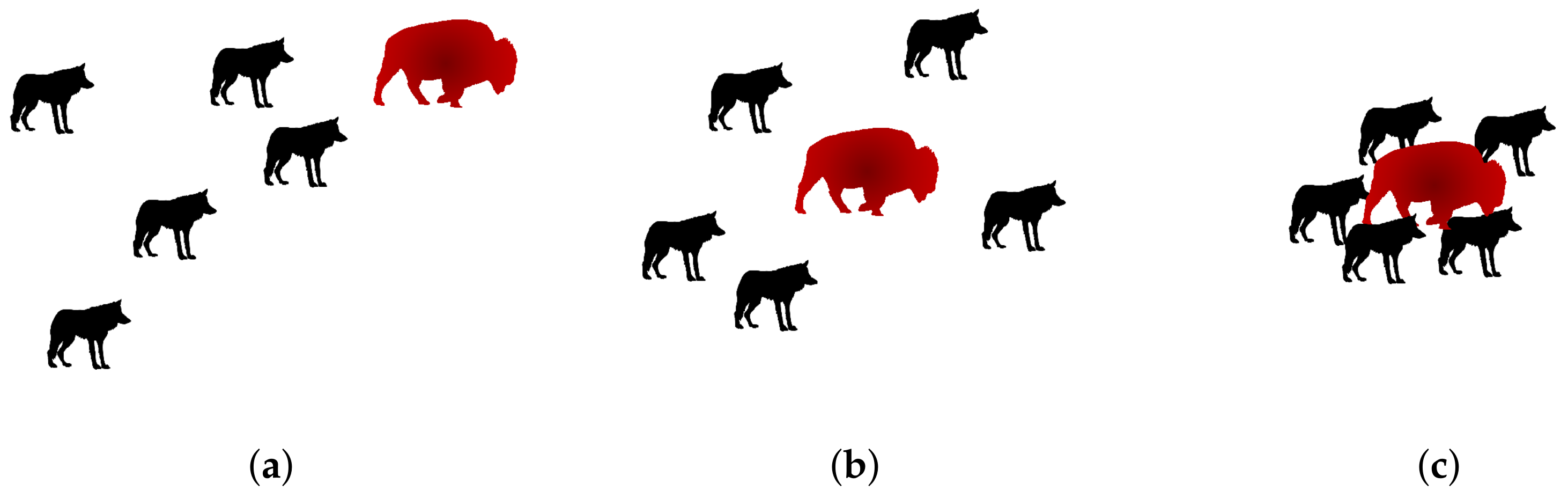
• Group hunting process: It is a collective process by the members of the pack that includes the prey encirclement (exploitation phase) and the prey hunting (exploration phase) (Figure 2).

The complete list of the key terms regarding the GWO language can be found in [36].

2.1.3. GWO Algorithm

The GWO adopts the processes of grey wolves (social hierarchy and group hunting) to perform the optimization process. Generally speaking, let us denote with $NP$ the number of population members, with D the number of decision variables to be optimized, with $MaxIt$ the number of maximum iterations, and with $\overrightarrow{V}$ the vector including the position of each member of the population. The $\alpha$, $\beta$, and $\delta$ wolves of the pack model the first (best) three solutions (members of the population with the best value of the objective function), whereas the $\omega$ members are the rest of the candidate solutions. If we define ${\overrightarrow{V}}_{wolf}$ as the position vector for each wolf of the pack with respect to the position vector of the prey (${\overrightarrow{V}}_{prey}$), which is the optimized position vector of the desired solution, GWO computes the position vectors of each member of the population employing the social hierarchy and the group hunting processes. Moreover, a set of coefficient vectors, which are used to define the position vector of each member of the population, adjust the search mechanism between the exploitation and the exploration phases of the algorithm. The coefficient vectors are computed by randomly distributed vectors.

Algorithm A1 (see Appendix A.1) outlines the previously described structure of the Grey Wolf Optimizer. During the initialization of the algorithm, its main parameters ($NP$, D, $MaxIt$, and boundaries) are selected based on the optimization problem. Furthermore, the position vectors ${\overrightarrow{V}}_{wolf}$, ${\overrightarrow{V}}_{\alpha }$, ${\overrightarrow{V}}_{\beta }$, and ${\overrightarrow{V}}_{\delta }$ are randomly defined. With respect to the position vector, each member of the population is ranked to determine the alpha ($\alpha$), beta ($\beta$), delta ($\delta$), and omega ($\omega$) wolves (social hierarchy process). At each iteration (group hunting process), two independent loops are taking place—the prey encirclement, and the prey hunting. In the first loop, the objective functions of all members are computed,

$$F_{obj}=F({\overrightarrow{V}}_{SI})$$

(1)

where F being the objective function of the optimization problem (in GWO $SI=wolf$). At the same time, the algorithm updates the position vectors of the first three categories of wolves according to their objective function values. During the second loop, the position vectors of $\omega$ wolves are updated based on the position vectors of the first three categories as follows

$${\overrightarrow{V}}_{wolf}=\frac{{\overrightarrow{V}}^I+{\overrightarrow{V}}^{II}+{\overrightarrow{V}}^{III}}{3}$$

(2)

where ${\overrightarrow{V}}^I$, ${\overrightarrow{V}}^{II}$, and ${\overrightarrow{V}}^{III}$ are given by

$$\begin{array}{c}\hfill \begin{array}{c}{\overrightarrow{V}}^I={\overrightarrow{V}}_{\alpha }-{\overrightarrow{R}}_{\alpha }^I·{\overrightarrow{W}}_{\alpha }\hfill \\ {\overrightarrow{V}}^{II}={\overrightarrow{V}}_{\beta }-{\overrightarrow{R}}_{\beta }^I·{\overrightarrow{W}}_{\beta }\hfill \\ {\overrightarrow{V}}^{III}={\overrightarrow{V}}_{\delta }-{\overrightarrow{R}}_{\delta }^I·{\overrightarrow{W}}_{\delta }\hfill \end{array}\end{array}$$

(3)

In (3), ${\overrightarrow{V}}_{\alpha }$, ${\overrightarrow{V}}_{\beta }$, and ${\overrightarrow{V}}_{\delta }$ are the position vectors of the $\alpha$, $\beta$, and $\delta$ wolves, respectively, while

$${\overrightarrow{W}}_n=|{\overrightarrow{R}}_n^{II}·{\overrightarrow{V}}_n-{\overrightarrow{V}}_{wolf}|n\in \{\alpha ,\beta ,\delta \}$$

(4)

and ${\overrightarrow{R}}_n^I=2c·{\overrightarrow{r}}_1-c$, ${\overrightarrow{R}}_n^{II}=2·{\overrightarrow{r}}_2$. Finally, the c parameter is equal to $c=2-i·\frac{2}{MaxIt}$, i being the index of the current iteration.

2.2. Whale Optimization Algorithm

Whale Optimization Algorithm (WOA) was published by Mirjalili and Lewis in 2016 [35]. The algorithm is considered a global optimizer and is classified to the nature-inspired category of meta-heuristics. The WOA mimics the social and hunting processes of humpback whales in the oceanic and marine environment.

2.2.1. WOA Natural Model

Humpback whales belong to a species of baleen whales. They are usually organized in groups and they migrate from tropical waters, for breeding and birthing, to polar waters for feeding. One of the fascinating characteristics of humpback whales is that they engage the bubble-net technique for their feeding process (Figure 3). They use vocalizations to communicate with each other and they create a net of bubbles in a spiral trajectory to circle the prey.

2.2.2. WOA Language

The term definitions of the WOA technique are outlined as follows

• Leader whale: In a group of humpback whales, the leader is the whale which is closest to the prey. In the optimization process, this is analogous to the population member with the best position vector.
• Prey: Prey is considered as the optimized position vector of the desired solution in the optimization process. Prey is actually the food for the humpback whales.
• Position vector: It is the vector of the coordinates of a humpback whale that models a solution of the optimization problem.
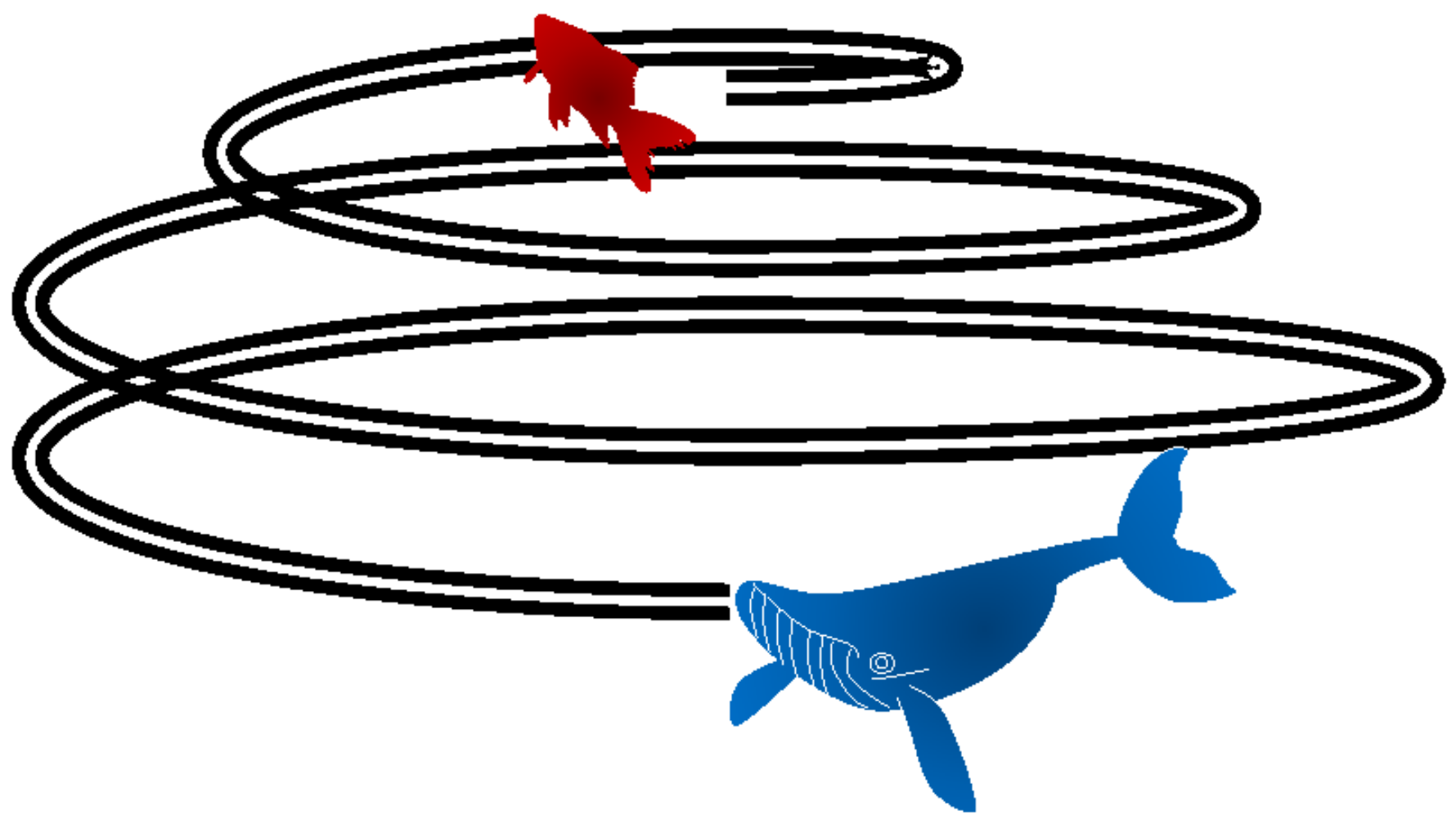
• Bubble-net feeding technique: It is a special hunting method applied by the humpback whales in their natural environment. It combines two different mechanisms. The first one is the swimming of the group towards the prey on a shrinking radius, while the second one includes the swimming of the group on a spiral trajectory towards the surface. The combination of these two mechanisms leads to prey entrapment by the humpback whales. Bubble-net feeding technique is the exploitation phase in the optimization process.

The complete list of key terms regarding the WOA language can be found in [35].

2.2.3. WOA Algorithm

The WOA mathematically models the process of humpback whales for searching and encircling the prey as well as for applying the bubble-net feeding technique. The WOA assumes that the best candidate solution is the desired prey and it updates the position vectors of the whales with respect to this optimal solution (prey encirclement). At each iteration, the population member with the best position vector is also updated if it scores a better solution. Extending the hunting behavior of humpback whales, WOA models the bubble-net feeding technique (exploitation phase) by combining simultaneously two different sub-processes: a shrinking radius-based prey encircling sub-process, where the members of the group are swimming towards the prey on a shrinking radius and an updating position vector sub-process based on a spiral trajectory, where the whales are swimming upwards in a spiral path to feed the trapped prey. It is worth mentioning that the bubble-net feeding of humpback whales is a cooperative technique. The members of the group have to learn the technique to be able to use it. As for the exploration phase, the WOA utilizes the same approach as in the prey encirclement to search for prey. To this end, the algorithm is adjusted by a set of randomly distributed coefficient vectors, suitable to balance the search mechanism between the exploration and the exploitation phase.

Algorithm A2 (see Appendix A.2) depicts the pseudo-code of the Whale Optimization Algorithm. After the initialization and at each iteration, the position vector ${\overrightarrow{V}}_{whale}$ of each member of the whales’ group is computed,

$$\begin{array}{c}\hfill {\overrightarrow{V}}_{whale}=\left\{\begin{array}{c}{\overrightarrow{V}}_{whale}^{rand}-{\overrightarrow{R}}^I·\overrightarrow{W}\hfill \\ {\overrightarrow{V}}_{leader}-{\overrightarrow{R}}^I·\overrightarrow{W}\hfill \\ \overrightarrow{W}·e^{p_1{p}_2}·cos(2\pi p_2)+{\overrightarrow{V}}_{whale}^{leader}\hfill \end{array}\right.\end{array}$$

(5)

where p, $p_1$, and $p_2$ are given by $p=rnd$, $p_1=1$, $p_2=(c_2-1)·rnd+1$ ($rnd$ is a random number $\in [0,1]$), $c_1$ and $c_2$ are coefficients given by $c_1=2-i·\frac{2}{MaxIt},c_2=-1+i·\frac{-1}{MaxIt}$, $\overrightarrow{W}$ is

$$\begin{array}{c}\hfill \overrightarrow{W}=\left\{\begin{array}{c}|{\overrightarrow{R}}^{II}·{\overrightarrow{V}}_{whale}^{rand}-{\overrightarrow{V}}_{whale}|\hfill \\ |{\overrightarrow{R}}^{II}·{\overrightarrow{V}}_{whale}^{leader}-{\overrightarrow{V}}_{whale}|\hfill \\ |{\overrightarrow{V}}_{whale}^{leader}-{\overrightarrow{V}}_{whale}|\hfill \end{array}\right.\end{array}$$

(6)

In (5) and (6), the first branch of the formula is applied in the exploration phase of the algorithm, the second branch in the prey encirclement, and the third branch in the bubble-net feeding technique based on the absolute value of the coefficient vector ${\overrightarrow{R}}^I$ and the value of the parameter p. These two values trigger one of these mechanisms at each i-th iteration of the WOA.

2.3. Salp Swarm Algorithm

The Salp Swarm Algorithm (SSA) and Multi-Objective Salp Swarm Algorithm (MSSA) were recently introduced by Mirjalili et al. [37] for solving single- and multi-objective optimization problems. The SSA algorithm mimics the behavior of salps in their natural environment (deep oceans).

2.3.1. SSA Natural Model

Salps are barrel-shaped, planktic tunicates categorized to the Salpida order. They have a gelatinous body (like jellyfishes) and to move in the oceanic environment they pump water through their body. Actually, this is a representative example of jet propulsion in nature. The literature on the behavior and the processes of salps swarms are very scarce. However, oceanographic researchers have recorded that in deep oceans, the individual salps are forming groups, which are called salps swarms or salps chains (Figure 4). These chains are of great importance within the life cycle of salps since they are able to reproduce and feed as members of the swarm.

2.3.2. SSA Language

The basic terms of the SSA language are displayed as follows

• Salp: It is a member of the population in a group of salps.
• Salp chain: It is a group of salps that swim in a chain-based formation to feed.
• Leader salp: It is the salp that is closest to the food in the oceanic environment and the first salp of a salp chain. In the optimization process, this is the member of the population with the best position vector.
• Followers salps: There are the salps that follow the leader salp in a chain.
• Position vector: It is the vector of the coordinates of a salp and it represents a solution to the optimization problem.

The complete list of the key terms regarding the SSA language can be found in [37].

2.3.3. SSA Algorithm

The SSA mathematically models the process of salps to form chains in the oceanic environment. The salps population is classified into two categories: the leader salp and the followers salps. As the definitions imply, the leader salp stands at the top of the chain, whereas the other salps follow. Apparently, the leader salp is the population member of the salps chain with the best position vector. If we define as ${\overrightarrow{V}}_{salp}$ the position vector for each salp of the swarm with respect to the position vector of the food (${\overrightarrow{V}}_{food}$), which is the optimized position vector of the desired solution, SSA computes the position vectors of each member of the salps population. Random coefficients adjust the search mechanism between exploration and exploitation.

Algorithm A3 (see Appendix A.3) presents the mathematical model in pseudo-code of the Salp Swarm Algorithm. The position vector of each salp in the chain ${\overrightarrow{V}}_{salp}$ is ranked to determine the position vector of the food (${\overrightarrow{V}}_{food}$). At each i-th iteration, the position vector of each salp is computed,

$$\begin{array}{c}\hfill {\overrightarrow{V}}_{salp}=\left\{\begin{array}{c}{\overrightarrow{V}}_{food}+p_1·(ub-lb)·p_2+lb,\mathrm{if}j\le NP/2\mathrm{and}{p}_3<0.5\hfill \\ {\overrightarrow{V}}_{food}-p_1·(ub-lb)·p_2+lb,\mathrm{if}j\le NP/2\mathrm{and}{p}_3\ge 0.5\hfill \\ \frac{{\overrightarrow{V}}_{salp,j}+{\overrightarrow{V}}_{salp,(j-1)}}{2},\mathrm{otherwise}\hfill \end{array}\right.\end{array}$$

(7)

where $p_1=2·e^{-{\left(\frac{4·i}{MaxIt}\right)}^2}$,  $p_2,p_3=rnd\in [0,1]$, $ub$ and $lb$ being the upper and the lower boundaries of the optimization problem. Consequently, the objective function value of each salp is computed $F({\overrightarrow{V}}_{salp})$ and compared to the objective function value of the food. Based on the comparison, the position vector of the food ${\overrightarrow{V}}_{food}$ as well as its corresponding objective function value, $F({\overrightarrow{V}}_{food})$, are updated.

3. Related Work

The GWO [36] has been successfully applied to various optimization problems in antenna design. A noticeable work effort has been published in the design of antenna arrays (linear and planar). Saxena and Kothari [47] applied the GWO algorithm to the design of linear antenna arrays. Their objective was to obtain an optimal pattern synthesis by optimizing the antenna elements position in a uniform excitation and by optimizing the current distribution of antenna elements assuming uniform array spacing and phase. The pattern synthesis of antenna arrays was investigated in [48]. The authors introduced a dynamic cooperative mechanism of weight factors to update the positions of the three wolves ($\alpha$, $\beta$, and $\delta$) in the GWO algorithm. Their objective was to improve the convergence speed of the original GWO to obtain feasible solutions in the pattern synthesis of linear antenna arrays. Numerical results demonstrated an improvement of the peak SLL (sidelobe level) and the deep null steering. The authors in [49] designed and optimized a thinned concentric circular antenna array by using the GWO. Their objective was to achieve patterns with more directive characteristics and with more accurate control of sidelobe levels. Simulated results showed satisfactory values of null depths and peak SLL. Khan et al. [50] utilized a hybrid GWO-IPA (Grey Wolf Optimizer [36]-Interior Point Algorithm [51]) algorithm to mitigate the resulting errors in the radiation power pattern of an antenna array. Simulated results demonstrated that the proposed fitness function corrects the pattern distortion in terms of sidelobe level and null depth level (NDL) as well as in null limitation. In [52], the authors investigated the design of a 100-element linear and a 100-element planar array by employing the GWO algorithm and other well-known algorithms (Genetic Algorithm (GA), Particle Swarm Optimization (PSO) [38], and Imperialist Competitive (IC) [53]). Their objective was to obtain an optimal solution when applying the array thinning method. Numerical results showed that the GWO algorithm outperformed the other algorithms in terms of minimizing the SLL for both linear and planar arrays. Lakhlef et al. [54] applied the GWO to re-adjust the amplitude and the phase of a linear antenna array when a failure or damage occurs to the desired pattern. To evaluate the durability of their proposed technique, different types of failures or damages were investigated. Their results proved the applicability and the effectiveness of the utilized algorithm in mitigating the failures of linear antenna arrays. In [55], the authors initially utilized the multi-objective GWO to address the problem of maximizing the transmission efficiency in wireless power transfer (WPT) systems. However, they verified the efficacy of their proposed technique on array antennas.

A noteworthy effort has been published utilizing the GWO algorithm in the design of compact antennas for next-generation communication systems. Li and Luk [56] investigated the synthesis of linear arrays by the use of the GWO algorithm. They extend their study in the presented algorithm, by optimizing the design of a dual-band E-shaped antenna and a wideband magneto-electric dipole antenna. Their findings indicated a satisfactory performance of the GWO compared to other well-known meta-heuristics (GA, PSO, Differential Evolution [15,57]). A patch antenna design operating in frequencies above 50 GHz was presented in [58]. The authors optimized the parameters (patch length, patch width, substrate thickness, and dielectric constant ${ϵ}_r$) of a patch antenna by applying the opposition-based GWO algorithm. Numerical results demonstrated satisfactory performance of the obtained antenna in terms of gain, radiation pattern, characteristic impedance, directivity, and efficiency. Boursianis et al. [59] applied the GWO algorithm to the design of a low-cost dual-band E-shaped patch antenna suitable for radio-frequency (RF) energy-harvesting (RH) applications. The proposed antenna design exhibited a satisfactory operation bandwidth for both frequency bands. Goudos et al. [60] introduced a novel hybrid algorithm based on Jaya [61] and GWO. Based on the proposed algorithm, the authors designed and fabricated two modified E-shaped circularly-polarized patch antennas operating in the 5G frequency bands of 3.7 GHz and 26 GHz. Simulated and measured results for both antennas were in good agreement. The presented antennas exhibited wideband operation in the desired frequency bands and satisfactory current distribution for circular polarization. The binary GWO has been applied in [62] to design and optimize an arbitrary-shaped dual-band patch antenna. Numerical results demonstrated the effectiveness of the utilized algorithm to the application of discrete-valued problems in antenna design. Finally, Rao et al. [63] designed and presented a Vivaldi antenna by applying an improved GWO to minimize the radar cross section (RCS), and therefore, to enhance the gain performance.

The WOA [35] has also been employed recently in various optimization problems of antenna design. The optimization problem of sidelobe suppression has been addressed in [64,65,66,67,68]. In detail, Yuan et al. [64] applied the WOA to the synthesis of a sparse antenna array. Their objective was to achieve a significantly lower peak sidelobe level (pSSL) value in the radiation pattern of the antenna array. Simulated results showed the effectiveness of the applied algorithm in the suppression of SLL. Zhang et al. [65,66] introduced the WOA to the synthesis of broadside linear aperiodic arrays with uniform excitation. From their presented results, the superiority of the WOA to suppress the pSLL combined with NDL is revealed, compared to other state-of-the-art algorithms. An improved WOA has been proposed in [67]. The authors applied the proposed algorithm to optimize the pattern of the MIMO radar system. Numerical results demonstrated the effectiveness of the algorithm and its ability to achieve pSLL and NDL at the desired levels. Additionally, the authors in [68] designed and optimized, in terms of amplitude, position and phase an antenna array structure in smart antenna technology by utilizing the WOA. Their objective was to obtain radiation patterns achievable SLL reduction by optimizing amplitude excitations, inter-element distances, and phases for each element of the array. Numerical results exhibited a relatively improved performance of the WOA against other popular algorithms.

The problem of error mitigation in the radiation pattern of an antenna array has also been addressed with the use of WOA in [69]. Patel et al. studied the failure correction of the radiation pattern in a linear array by applying the WOA and the Chaotic WOA (CWOA). Simulated results showed the efficacy of the algorithm to re-optimize the amplitude excitations of powered elements in a failed antenna array. A modified WOA has been employed by [70] for pattern synthesis of a linear antenna array. Computed results demonstrated the efficacy of the selected algorithm against other popular algorithms in the literature. The problem of scattering in a MIMO system is also of importance since it is related to the system channel capacity. The authors in [71] designed and optimized an antenna element of a MIMO system by applying a binary WOA with a crossover operator. Numerical results demonstrated the improvement of system capacity even for poor scattering environments. Moreover, the WOA has been utilized in the design of compact and planar antennas. In [72], the authors applied the WOA as an optimization technique to design and fabricate a quad H-slotted antenna at ISM (Industrial Scientific Medicine) frequency band of 2.45 GHz. The authors in [73] applied the WOA to design a planar inverted-F antenna (PIFA) for wearable wireless applications. Numerical results exhibited the validity of the proposed design structure. An equivalent circuit model based on the WOA has been presented in [74] to design a dual-band frequency selective surface (FSS) for WLAN shielding applications. Computed and measured results exhibited the effectiveness of the utilized algorithm to the given optimization problem. Finally, Singh et al. has employed the WOA to design and fabricate a Fibonacci fractal planar antenna [75] and a modified triangular patch antenna array [76], both operating in the 4.9 GHz frequency band for public safety applications. Numerical and measured results demonstrated the acceptable performance of the proposed antennas.

As far as the SSA [37] is concerned, various efforts in antenna design optimization are found in the literature. Prabhakar and Satyanarayana [77] combined the SSA and the WOA to propose a new hybrid algorithm in order to address the problem of pattern synthesis in a conformal antenna array. The proposed hybrid algorithm is evaluated through a series of several well-known test functions. Numerical results demonstrated satisfactory performance of the proposed method and the reported amplitude and phase excitations versus the element number of the conformal array exhibit an improvement compared with previous research works. An improved SSA has been employed in [78] to address the problem of optimizing circular arrays with a mutual coupling effect. The presented results demonstrated an improvement in the overall performance of the designed circular arrays. The authors in [79] applied the SSA to design linear and planar sparse antenna arrays by optimizing the SLL. The results proved the efficacy of the selected algorithm. The authors in [80] optimized a MIMO antenna operating in 5G n257 frequency band by utilizing the SSA. Preliminary results exhibited the broadband operation combined with the small size of the proposed MIMO antenna in the frequency band of interest. The problem of antenna array synthesis on the thinning of concentric circular structures has been addressed by the use of binary SSA in [81]. The authors utilized the binary SSA approach to decrease the maximum SLL of a concentric circular array by keeping the percentage of thinning higher than 50%. Finally, the authors in [82] optimized a modified E-shaped patch antenna for RF energy harvesting applications by applying the SSA technique. The optimized antenna was operated in the frequency bands of 4G and 5G mobile communication systems and the numerical results demonstrated satisfactory performance of the proposed antenna as a receiving module in a rectenna system.

Table 1. Summary of optimization problems and the corresponding algorithms.

Opt. Problem	SI Algorithm	References
Antenna array	GWO, WOA, SSA	[47,48,49,52,54,55,56,64,65,66,68,70,77,78,79,81]
Radiation pattern	GWO, WOA	[50,69]
Antenna design	GWO, WOA, SSA	[56,58,59,60,62,63,72,73,74,75,76,82]
MIMO system	WOA, SSA	[67,71,80]

summarizes the related work that has been published in the literature grouped by the three selected SI algorithms.

4. Numerical Results

In this section, we evaluate the performance of the GWO, the SSA, and the WOA algorithms by utilizing several benchmark functions. We extend the algorithms’ assessment by optimizing various antenna design problems. A comparative study among these three algorithms is carried out in conjunction with the well-known Particle Swarm Optimization (PSO), Artificial Bee Colony (ABC), and Firefly Algorithm (FA). For the performance evaluation, we utilize custom tools developed in MATLAB (© 1994–2020, The MathWorks, Inc., Natick, MA, USA). Finally, the commercial high-frequency electromagnetic solver (HFSS, © 2020 ANSYS, Inc., Canonsburg, PA 15317, USA) is combined with the implementation of the WOA in MATLAB environment.

4.1. Algorithms Performance

Firstly, a set of several widely-known benchmark functions is applied. These benchmark functions include two uni-modal functions, namely the Sphere function and Rosenbrock’s function. Eight multi-modal functions are also included for the evaluation of the SI algorithms, namely the Ackley’s, Griewanks’s, Weierstrass, Rastrigin’s, Noncontinuous Rastrigin’s, Schwefel’s, Generalized Penalized, and Generalized Penalized 2 functions. The global minima of all the above functions are zero. The definitions of these functions are given in the literature [60,83]. The dimensionality D of all benchmark functions is set to 60. For all algorithms, we apply the number of iterations $MaxIt$ to 1000, the population size $NP$ to 100, and the number of independent trials to 50.

Table 2. Numerical results (average values) of the emerging SI algorithms (GWO, SSA, WOA) and PSO, ABC, FA for several benchmark functions (D = 60, best values are indicated in bold).

Benchmark Function	Algorithm
	GWO	SSA	WOA	PSO	ABC	FA
Sphere	1.51 $\times {10}^{-55}$	4.65 $\times {10}^{-08}$	2.89 $\times {\mathbf{10}}^{-\mathbf{165}}$	2.64 $\times {10}^{-05}$	1.42 $\times {10}^{-07}$	5.42 $\times {10}^{-07}$
Rosenbrock	5.64 $\times {10}^{+01}$	5.79 $\times {10}^{+01}$	5.30 $\times {10}^{+01}$	5.17 $\times {\mathbf{10}}^{+\mathbf{01}}$	5.85 $\times {10}^{+01}$	1.65 $\times {10}^{+02}$
Ackley	2.54 $\times {10}^{-14}$	2.45 $\times {10}^{+00}$	3.84 $\times {\mathbf{10}}^{-\mathbf{15}}$	6.23 $\times {10}^{+00}$	4.64 $\times {10}^{-03}$	2.07 $\times {10}^{+00}$
Generalized Griewank	1.10 $\times {10}^{-03}$	5.62 $\times {10}^{-03}$	1.20 $\times {10}^{-03}$	1.73 $\times {10}^{-01}$	2.73 $\times {\mathbf{10}}^{-\mathbf{04}}$	2.21 $\times {10}^{-02}$
Weierstrass	1.71 $\times {10}^{-15}$	2.52 $\times {10}^{+01}$	0.00 $\times {\mathbf{10}}^{+\mathbf{00}}$	2.56 $\times {10}^{+01}$	2.96 $\times {10}^{-02}$	2.23 $\times {10}^{+01}$
Generalized Rastrigin	4.18 $\times {10}^{-01}$	6.43 $\times {10}^{+01}$	0.00$\times {\mathbf{10}}^{+\mathbf{00}}$	1.45 $\times {10}^{+02}$	1.59 $\times {10}^{+01}$	3.56 $\times {10}^{+02}$
Noncont. Rastrigin	1.48 $\times {10}^{+00}$	9.94 $\times {10}^{+01}$	0.00$\times {\mathbf{10}}^{+\mathbf{00}}$	1.21 $\times {10}^{+02}$	1.88 $\times {10}^{+01}$	3.74 $\times {10}^{+02}$
Schewfel	1.45 $\times {10}^{+04}$	1.03 $\times {10}^{+04}$	8.90 $\times {\mathbf{10}}^{+\mathbf{02}}$	1.09 $\times {10}^{+04}$	4.68 $\times {10}^{+03}$	1.21 $\times {10}^{+04}$
Generalized Penalized 1	5.59 $\times {10}^{-02}$	4.98 $\times {10}^{+00}$	3.60$\times {\mathbf{10}}^{-\mathbf{04}}$	7.03 $\times {10}^{-01}$	4.42 $\times {10}^{-03}$	8.44 $\times {10}^{+00}$
Generalized Penalized 2	1.44 $\times {10}^{+00}$	2.04 $\times {10}^{+01}$	1.40$\times {\mathbf{10}}^{-\mathbf{02}}$	3.22 $\times {10}^{-02}$	7.41 $\times {10}^{-02}$	4.16 $\times {10}^{+00}$

lists the results (average values of 50 independent trials) of the comparative study. We can easily notice that WOA finds the best results in eight out of the 10 test functions. GWO performs a higher score, as compared to the rest of the algorithms, in two test functions; only one test function achieves better results with PSO.

4.2. Linear Antenna Array Design

The next step is to evaluate the selected SI algorithms by utilizing the optimization problem of linear array design. Generally speaking, the synthesis of antenna arrays in wireless communication systems is of significant importance. In this context, the sidelobe level suppression is a typical optimization task in antenna arrays. Hence, the synthesis of antenna arrays is one of the most classic, yet demanding, optimization problems that have been thoroughly studied in the literature by utilizing various analytical or stochastic techniques [19,84,85,86,87,88,89]. The vast majority of the well-known array synthesis techniques, including the Dolph–Chebyshev and Taylor methods, work only for equally spaced array elements and produce real amplitude. However, these methods produce large amplitude ratios that cause spurious radiations originating from the feed, thus mitigating the desired radiation pattern. Another drawback when designing antenna arrays with a non-uniform amplitude is the total radiated power. If we consider a specific number of elements in the antenna array design and take into account the total radiated power, we can conclude that the amplitude taper in the elements cannot generate an optimum design due to the functionality of the total power of the array elements [26].

Instead, if we apply uniform amplitudes in all the elements of the antenna array and vary the phases of the generated signals, the total radiated power in the broadside direction can be maximized [26]. Therefore, the use of phase-only synthesis is a better alternative technique to a non-uniform amplitude array for various wireless applications. However, if we use phase-only synthesis with equal inter-element spacing, then a larger number of elements is required to achieve a similar sidelobe level as the corresponding non-uniform amplitude array. This drawback can be bypassed using an array with unequally spaced elements and unequal phases, thus optimizing both positions and phases of the elements in an array, as it is described in [26,90]. Nevertheless, in this case, the nonlinear and non-convex dependence of the array factor based on the element positions and phases imposes a significant step of difficulty in the synthesis of unequally spaced arrays. This type of problem is challenging and the use of a global optimization method like the evolutionary or the SI algorithms is a promising solution to address it.

Taking into account all the above, let us consider an N-element linear array, where its elements are symmetrically placed along the x-axis (see Figure 5). Along the $xz$ plane, the array factor can be expressed as

$$AF(\overrightarrow{y},\overrightarrow{\varphi },\overrightarrow{A},\vartheta )=\sum _{n=1}^N{A}_n{e}^{j\left(\frac{2\pi }{\lambda }{y}_{n}sin\vartheta +{\varphi }_n\right)}$$

(8)

where $\lambda$ is the wavelength of the incident field, $\vartheta$ is the steering angle that is computed along the z-axis (towards positive direction), $\overrightarrow{y}$, $\overline{A}$, and $\overline{\varphi }$ are the position, amplitude, and phase vectors of the linear array, and $y_n$, $A_n$, and ${\varphi }_n$ are the corresponding scalar quantities of the aforementioned vectors of the n-th element, accordingly. Assuming a symmetrical and uniformly excited array, the array factor in the $xz$ plane can be rewritten as

$$AF(\overrightarrow{y},\overrightarrow{\varphi },\vartheta )=2\sum _{m=1}^{M}cos\left[\frac{2\pi }{\lambda }{y}_{m}sin\vartheta +{\varphi }_m\right]$$

(9)

Equation (9) can be written in dB as

$$A{F}_{\mathrm{dB}}\left(\overrightarrow{y},\overrightarrow{\varphi },\vartheta \right)=20·{log}_{10}\left|\frac{AF\left(\overrightarrow{y},\overrightarrow{\varphi },\vartheta \right)}{AF\left(\overrightarrow{y},\overrightarrow{\varphi },{\vartheta }_o\right)}\right|$$

(10)

where ${\vartheta }_o$ is the direction of the maximum. The position of the elements in this array meets the following criteria

$$\begin{array}{cc}\hfill y_1\ge \frac{d_{min}}{2}& ,y_1\le \frac{d_{max}}{2}\hfill \\ \hfill \left\{\begin{array}{c}\left|y_m-y_{m+1}\right|\ge d_{min}\hfill \\ \left|y_m-y_{m+1}\right|\le d_{max}\hfill \end{array}\right\}& ,1\le m\le M-1\hfill \end{array}$$

(11)

where $y_1$ is the position of the first element, $y_m$ is the position of the m element, $y_{m+1}$ is the position of the $m+1$ element, and $d_{min}$, $d_{max}$ are the minimum and maximum inter-element spacing, accordingly.

Taking into consideration the above formulation, one of the most common objectives in antenna design is to suppress the SLL of the linear array. This objective can be carried out by finding the optimum positions and phases of the elements in the array. Therefore, this type of problem can be recast as an optimization one by minimizing the following objective function

$$F(\overrightarrow{y},\overrightarrow{\varphi })={max}_{\vartheta \in T}\left\{A{F}_{dB}(\overrightarrow{y},\overrightarrow{\varphi },\vartheta )\right\}$$

(12)

where T is the set of theta angle values that fall outside the angular range of the main lobe of the linear array.

Generally speaking, the formulation of the directivity of the linear array in (8) can be expressed as [91]

$$D=\frac{{\left({\displaystyle \sum _{m=-M}^M}{A}_m\right)}^2}{{\displaystyle \sum _{m=-M}^M}{\displaystyle \sum _{n=-M}^M}{A}_n{A}_m{e}^{j\left({\varphi }_m-{\varphi }_n\right)}\frac{sin\left[\frac{2\pi }{\lambda }\left(y_m-y_n\right)\right]}{\frac{2\pi }{\lambda }\left(y_m-y_n\right)}}$$

(13)

For a uniformly excited linear array, (13) can be simplified to

$$D=\frac{4M^2}{{\displaystyle \sum _{m=-M}^M}{\displaystyle \sum _{n=-M}^M}{e}^{j\left({\varphi }_m-{\varphi }_n\right)}\frac{sin\left[\frac{2\pi }{\lambda }\left(y_m-y_n\right)\right]}{\frac{2\pi }{\lambda }\left(y_m-y_n\right)}}$$

(14)

In this work, we investigate the case of a 50-element linear array as a position-phase synthesis of uniformly excited arrays. We set $d_{min}$ = 0.5$\lambda$ and $d_{max}$ = $\lambda$, where $d_{min}$ is the minimum and $d_{max}$ is the maximum allowable inter-element distance, accordingly. The number of unknowns in our case is $2M$. The array phases vary from $0^{\circ }$ to ${360}^{\circ }$. The optimization problem is highly dimensional with D = 100 decision variables. The population size $NP$ is also set to 100, whereas the maximum number of iterations $MaxIt$ is set to 1000. Finally, all algorithms are applied for 50 independent trials. The corresponding equally spaced uniform array of 50 elements exhibits an SLL value of −18.65 dB and directivity of 16.99 dB.

Table 3. Comparative results (pSLL values) for the position-phase synthesis of a 50-element linear array (best values are indicated in bold, all values are expressed in dB).

Algorithm	Best	Worst	Mean	Median	Std. Dev.
GWO	−24.22	−20.65	−23.16	−23.19	0.69
SSA	−23.62	−14.30	−17.34	−15.41	3.13
WOA	−21.86	−17.23	−19.11	−19.05	1.04
PSO	−23.73	−14.63	−18.74	−18.79	1.78
ABC	−18.48	−17.69	−18.04	−17.97	0.22
FA	−18.62	−16.88	−17.97	−18.04	0.47

lists the comparative results of the 50-element linear array design case. From the presented results, we can conclude that GWO achieves the highest score compared to all other algorithms. PSO obtained the second best array design. Figure 6a illustrates the distribution of the results in percentiles (boxplot). From the obtained results, we can deduce that the GWO achieves the best 50% percentile (median value) of the cost function compared to the rest of the algorithms values. The worst result is obtained by the SSA. It is also noteworthy that the upper and lower values of the PSO distribution are similar to the values of the SSA distribution. Figure 6b depicts the average convergence rate of the algorithms under study. We can derive that GWO and WOA algorithms obtain the fastest convergence, whereas SSA and PSO algorithms converge more slowly. The radiation patterns of the best-obtained array design are portrayed in Figure 6c. From the presented graph, we can conclude that the best array design is found by applying the GWO algorithm. The peak SLL value of the best linear array design is −24.22 dB and the directivity is 17.85 dB. Therefore, the obtained results by the optimization process exhibit an improvement both in the SLL and directivity values of about 6 dB and 1 dB, accordingly, when compared to the values of the corresponding uniformly excited linear array.

4.3. Non-Parametric Statistical Tests

To further assess and quantify the performance of the algorithms, we carry out non-parametric statistical tests [92,93]. Firstly, we apply the Friedman test to the average values of the benchmark functions (Table 2), and the average values of the array design case (Table 3). The algorithm ranking results obtained by the Friedman test are listed in

Table 4. Numerical results obtained by Friedman test (highest ranking is indicated in bold).

Algorithm	GWO	SSA	WOA	PSO	ABC	FA
Average Ranking	2.50	4.42	1.42	4.50	3.00	5.17

. We can easily conclude that WOA achieves the highest rank among all other algorithms under test. GWO scores the second-highest rank, whereas FA has the lowest ranking.

Furthermore, the Wilcoxon signed-rank test with a significance level of p = 0.05 is conducted to further evaluate the differences between WOA and the rest of the algorithms under study.

Table 5. Numerical results obtained by Wilcoxon signed-rank test (values below significant level are indicated in bold).

WOA vs.	GWO	SSA	PSO	ABC	FA
p-value	6.93 × 10−02	4.88 × 10−04	1.95 × 10−03	7.32 × 10−03	4.88 × 10−04

reports the obtained test results. One may notice that WOA achieves the highest rank among all the algorithms, but GWO. Although the WOA cannot be considered as significantly better than the original GWO, (yet being significantly better than the SSA, the PSO, the ABC, and the FA algorithm), it outperforms the rest of the given algorithms according to the average ranking results.

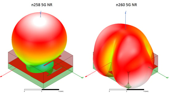
4.4. 5G Antenna Design

With the advent of fifth-generation (5G) and its forthcoming operation in millimeter-wave frequency bands of mobile communication networks, certain requirements, such as wide and ultra-wide spectrum, multi-band operation, and data rates in the order of Gigabits-per second (Gbps), will change drastically the specifications in antenna design. The use of microstrip patch antennas in millimeter-wave frequency bands is a candidate solution to provide efficacious and robust designs. In the literature, there are several efforts in designing antennas for millimeter-wave frequency bands of 5G mobile communication systems [94,95]. E-shaped patch antennas can extend the operation and functionality of patch antennas in dual- or multi-frequency bands [31,32,33]. Their design is subjected to the following constraints [31,90]

$$\begin{array}{cc}\hfill L_{slot1}& <L_{antenna}\hfill \\ \hfill L_{slot2}& <L_{antenna}\hfill \\ \hfill \frac{D_{slot}}{2}+W_{slot}& <\frac{W_{antenna}}{2}\hfill \end{array}$$

(15)

where $L_{slot1}$ is the length of the first slot in the E-shaped antenna, $L_{slot2}$ is the length of the second slot, $L_{antenna}$ is the length of the E-shaped antenna, $W_{slot}$ is the width of the slot, $W_{antenna}$ is the width of the E-shaped antenna, and $D_{slot}$ is the distance of the slot from the center of the E-shaped antenna.

One of the challenging tasks in antenna design is the choice of the feeding technique. Besides classical feeding techniques, such as coaxial or microstrip feeding, shaped aperture-coupled feeding has gained noticeable interest due to the comparative characteristics that can provide, i.e., dual- or multi-band operation, wide and ultra-wide bandwidth, dual-polarization mode, and high gain values [96,97,98,99]. Shaped aperture-coupled feeding can be also applied in millimeter-wave frequency band antennas [100]. However, for the patch antenna to achieve a dual-band operation when using aperture-coupled feeding, the shape of the aperture should be modified. A representative example of aperture shape modification to achieve dual-band operation in patch antenna design has been presented in [33].

Design methods for aperture-coupled patch antennae have been presented in [101]. These guidelines are applied for evaluation to design two different cases of an aperture-coupled patch antenna in the millimeter-wave frequency bands. The selected frequencies of the evaluation fall into the n258 (center frequency: 26.4 GHz) and n260 (center frequency: 38.5 GHz) 5G NR frequency bands.

Table 6. Extracted parameter values as they obtained from the design method presented in [101], ${\lambda }_1$ is the wavelength of the antenna dielectric, and ${\lambda }_2$ is the wavelength of the feed dielectric (computed values are expressed in mm).

Parameter	Nominal Values [101]	UC1 26.4 GHz	UC2 38.5 GHz
$W_{antenna}$	$0.422{\lambda }_1$	3.23	2.21
$L_{antenna}$	$0.317{\lambda }_1$	2.42	1.66
$W_{feed}$	Feed line width for $50\mathsf{\Omega }$	0.59	0.59
$L_{feed}$	$0.739{\lambda }_2$	4.57	3.13
$L_{aperture}$	$0.148{\lambda }_1$	1.13	0.78
$W_{aperture}$	$0.016{\lambda }_1$	0.12	0.08
$O_{aperture}$	$0.211{\lambda }_2$	1.30	0.89

lists the extracted parameter values as they obtained from the design method described in [101]. Moreover, Figure 7 displays the perspective views (Figure 7a,b) and the computed results of the reflection coefficient as a function of frequency (Figure 7c) for the two different use cases of an aperture-coupled patch antenna in the millimeter-wave frequency bands. From the presented results, it is evident that the design method that was introduced in [101] cannot be applied in the millimeter-wave frequency bands. Both of the use cases (Figure 7a,b) do not resonate at the desired frequencies of the 5G NR bands. Moreover, the method in [101] cannot provide an efficient way of designing a patch antenna that performs in a dual-frequency band mode. Finally, taking into consideration the antenna complexity and the requirements of 5G NR frequency bands in antenna design, it seems that an optimization method is a straightforward process to obtain feasible solutions of antenna design in the aforementioned frequency bands if we recast this problem as an optimization one.

In this work, we present the optimization problem of an aperture-coupled E-shaped antenna operating in the n258 (center frequency: 26.4 GHz) and n260 (center frequency: 38.5 GHz) 5G NR frequency bands is investigated. The antenna is designed on a multi-layer approach (from bottom to top: feed-line, substrate, ground plane, substrate, E-shaped antenna) and optimized (the objects included in the optimization process is the E-shaped antenna and the feed line). It consists of a double dielectric substrate layer; the bottom one consists of Arlon 25N (${ϵ}_r$ =  3.38, $tan\delta$ =  0.0025) with 0.762 mm thickness and the top one consists of Taconic (${ϵ}_r$ =  2.21, $tan\delta$ =  0.001) with 1.58 mm thickness. An aperture is placed between the bottom and top substrate layers to feed the E-shaped antenna. Moreover, a modified ground plane is utilized to enhance the characteristics of the antenna. Figure 8 illustrates the proposed antenna geometry indicating the required design parameters.

To solve the design problem of the aperture-coupled E-shaped patch antenna, an optimization technique is required. The proposed antenna consists of 15 different design parameters. We address this problem by applying the Whale Optimization Algorithm (WOA) [35] as the optimization method. The selected algorithm is incorporated with the HFSS electromagnetic (EM) solver. The integration of the WOA source code with the EM solver is achieved using an HFSS MATLAB API wrapper. The optimization problem can be defined by the following objective function

$$\begin{array}{c}\hfill \begin{array}{c}F(\overrightarrow{y})=max(S_{11}^{26.4GHz}(\overrightarrow{y}),S_{11}^{38.5GHz}(\overrightarrow{y}))+\mathsf{\Psi }\times max(0,S_{11}^{26.4GHz}(\overrightarrow{y})-L_{dB})\hfill \\ +\mathsf{\Psi }\times max(0,S_{11}^{38.5GHz}(\overrightarrow{y})-L_{dB})\hfill \end{array}\end{array}$$

(16)

where $\overline{y}$ is the vector containing the antenna geometry variables for each solution, $S_{11}^{26.4GHz}$ and $S_{11}^{38.5GHz}$ are the desired $S_{11}$ magnitudes, $L_{dB}$ is the $S_{11}$ limit in dB, and $\mathsf{\Psi }$ is a penalty number (10⁺¹⁰). In our case, we set $L_{dB}$ = −10 dB.

Table 7. Best values of the design parameters obtained by the WOA (all values are given in mm).

Parameter	Value	Parameter	Value	Parameter	Value
$W_{antenna}$	4.14	$L_{antenna}$	2.86	$W_{slot}$	1.40
$L_{slot1}$	0.77	$L_{slot2}$	0.91	$D_{slot}$	1.04
$W_{ground}$	4.90	$L_{ground}$	5.86	$W_{ap}$	4.14
$L_{ap}$	1.09	$W_{slit}$	0.14	$L_{slit}$	2.46
$O_{ap}$	0.88	$W_{feed}$	1.09	$L_{feed}$	3.71

summarizes the best values of the design parameters obtained by the WOA.

Figure 9 depicts the $S_{11}$ magnitude of the aperture-coupled E-shaped patch antenna versus frequency. From the presented graph, we can derive that the obtained antenna operates satisfactorily in the n258 and n260 5G NR frequency bands. The antenna has a dual-frequency tuning operation (−44.71 dB at 26.54 GHz and −29.02 dB at 38.61 GHz) within the frequency bands of 5G NR (n258 and n260). It is worth mentioning that the −10 dB bandwidth of the obtained antenna practically covers the whole previously mentioned 5G frequency bands of interest.

Moreover, Figure 10 portrays the 3D pattern of the antenna gain (realized gain) achieved by the WOA at 26.4 GHz (Figure 10a) and 38.5 GHz (Figure 10b). It is worth noting that the maximum gain is 7.13 dB at 26.4 GHz and 4.95 dB at 38.5 GHz.

Finally, Figure 11 illustrates the surface current distribution of the optimized antenna design. From the presented results, we can obtain that the surface current is maximized mostly at the center area of the E-shaped patch and minimized at the edges of the antenna.

5. Conclusions

In this paper, three emerging swarm intelligence algorithms, namely the GWO, the WOA, and the SSA were investigated. To this end, several well-known test functions were utilized to assess the performance of the selected algorithms. Moreover, two different design cases, the design of a 50-element linear antenna array and the design of an aperture-coupled E-shaped patch antenna, were carried out to evaluate the operation of the SI algorithms. To further estimate their effectiveness, two independent statistical tests were applied, the Friedman test and the Wilcoxon signed-rank test. Numerical results demonstrated that the WOA outperforms the other algorithms in terms of average ranking as well as in 8 out of 10 well-known test functions. From the design case of the linear antenna array, we concluded that the best pSLL value was achieved by the GWO algorithm; yet the other SI algorithms exhibited satisfactorily competitive results. The employment of the WOA to the optimization problem of an aperture-coupled E-shaped antenna revealed the capability of the algorithm to design complex (a large number of parameters to be optimized) and compact (small size) structures as applications in antenna design optimization problems.

References

1. Rappaport, T.S.; Sun, S.; Mayzus, R.; Zhao, H.; Azar, Y.; Wang, K.; Wong, G.N.; Schulz, J.K.; Samimi, M.; Gutierrez, F. Millimeter Wave Mobile Communications for 5G Cellular: It Will Work! IEEE Access 2013, 1, 335–349. [Google Scholar] [CrossRef]
2. Gupta, A.; Jha, R.K. A Survey of 5G Network: Architecture and Emerging Technologies. IEEE Access 2015, 3, 1206–1232. [Google Scholar] [CrossRef]
3. O’Connell, E.; Moore, D.; Newe, T. Challenges Associated with Implementing 5G in Manufacturing. Telecom 2020, 1, 48–67. [Google Scholar] [CrossRef]
4. Ban, Y.L.; Li, C.; Sim, C.Y.D.; Wu, G.; Wong, K.L. 4G/5G Multiple Antennas for Future Multi-Mode Smartphone Applications. IEEE Access 2016, 4, 2981–2988. [Google Scholar] [CrossRef]
5. Boccardi, F.; Heath, R.W.; Lozano, A.; Marzetta, T.L.; Popovski, P. Five disruptive technology directions for 5G. IEEE Commun. Mag. 2014, 52, 74–80. [Google Scholar] [CrossRef] [Green Version]
6. Abulgasem, S.; Tubbal, F.; Raad, R.; Theoharis, P.I.; Lu, S.; Iranmanesh, S. Antenna Designs for CubeSats: A Review. IEEE Access 2021, 9, 45289–45324. [Google Scholar] [CrossRef]
7. Lee, K.F.; Luk, K.M.; Lai, H.W. Microstrip Patch Antennas; World Scientific: Singapore, 2017. [Google Scholar]
8. Goudos, S.K. Emerging Evolutionary Algorithms for Antennas and Wireless Communications; Electromagnetic Waves; SciTech Publishing: Stevenage, UK, 2021. [Google Scholar]
9. Abdel-Basset, M.; Abdel-Fatah, L.; Sangaiah, A.K. Chapter 10-Metaheuristic Algorithms: A Comprehensive Review. In Computational Intelligence for Multimedia Big Data on the Cloud with Engineering Applications; Sangaiah, A.K., Sheng, M., Zhang, Z., Eds.; Intelligent Data-Centric Systems; Academic Press: Cambridge, MA, USA, 2018; pp. 185–231. [Google Scholar] [CrossRef]
10. Wolpert, D.H.; Macready, W.G. No free lunch theorems for optimization. IEEE Trans. Evol. Comput. 1997, 1, 67–82. [Google Scholar] [CrossRef] [Green Version]
11. Haupt, R. An introduction to genetic algorithms for electromagnetics. IEEE Antennas Propag. Mag. 1995, 37, 7–15. [Google Scholar] [CrossRef] [Green Version]
12. Johnson, J.; Rahmat-Samii, V. Genetic algorithms in engineering electromagnetics. IEEE Antennas Propag. Mag. 1997, 39, 7–21. [Google Scholar] [CrossRef] [Green Version]
13. Jin, N.; Rahmat-Samii, Y. Advances in particle swarm optimization for antenna designs: Real-number, binary, single-objective and multiobjective implementations. IEEE Trans. Antennas Propag. 2007, 55, 556–567. [Google Scholar] [CrossRef]
14. Robinson, J.; Rahmat-Samii, Y. Particle swarm optimization in electromagnetics. IEEE Trans. Antennas Propag. 2004, 52, 397–407. [Google Scholar] [CrossRef]
15. Rocca, P.; Oliveri, G.; Massa, A. Differential Evolution as Applied to Electromagnetics. IEEE Antennas Propag. Mag. 2011, 53, 38–49. [Google Scholar] [CrossRef]
16. Ares-Pena, F.; Rodriguez-Gonzalez, J.; Villanueva-Lopez, E.; Rengarajan, S. Genetic algorithms in the design and optimization of antenna array patterns. IEEE Trans. Antennas Propag. 1999, 47, 506–510. [Google Scholar] [CrossRef]
17. Marcano, D.; Duran, F. Synthesis of antenna arrays using genetic algorithms. IEEE Antennas Propag. Mag. 2000, 42, 12–20. [Google Scholar] [CrossRef]
18. Yan, K.K.; Lu, Y. Sidelobe reduction in array-pattern synthesis using genetic algorithm. IEEE Trans. Antennas Propag. 1997, 45, 1117–1122. [Google Scholar] [CrossRef]
19. Haupt, R. Thinned arrays using genetic algorithms. IEEE Trans. Antennas Propag. 1994, 42, 993–999. [Google Scholar] [CrossRef]
20. Yeo, B.K.; Lu, Y. Array failure correction with a genetic algorithm. IEEE Trans. Antennas Propag. 1999, 47, 823–828. [Google Scholar] [CrossRef]
21. Khodier, M.; Christodoulou, C. Linear array geometry synthesis with minimum sidelobe level and null control using particle swarm optimization. IEEE Trans. Antennas Propag. 2005, 53, 2674–2679. [Google Scholar] [CrossRef]
22. Bevelacqua, P.J.; Balanis, C.A. Minimum Sidelobe Levels for Linear Arrays. IEEE Trans. Antennas Propag. 2007, 55, 3442–3449. [Google Scholar] [CrossRef]
23. Boeringer, D.; Werner, D. Particle swarm optimization versus genetic algorithms for phased array synthesis. IEEE Trans. Antennas Propag. 2004, 52, 771–779. [Google Scholar] [CrossRef]
24. Goudos, S. Antenna Design Using Binary Differential Evolution: Application to discrete-valued design problems. IEEE Antennas Propag. Mag. 2017, 59, 74–93. [Google Scholar] [CrossRef]
25. Caorsi, S.; Massa, A.; Pastorino, M.; Randazzo, A. Optimization of the difference patterns for monopulse antennas by a hybrid real/integer-coded differential evolution method. IEEE Trans. Antennas Propag. 2005, 53, 372–376. [Google Scholar] [CrossRef]
26. Kurup, D.; Himdi, M.; Rydberg, A. Synthesis of uniform amplitude unequally spaced antenna arrays using the differential evolution algorithm. IEEE Trans. Antennas Propag. 2003, 51, 2210–2217. [Google Scholar] [CrossRef]
27. Yang, S.; Gan, Y.; Qing, A. Antenna-array pattern nulling using a differential evolution algorithm. Int. J. Microw. Comput.-Aided Eng. 2004, 14, 57–63. [Google Scholar] [CrossRef]
28. Panduro, M.A.; Brizuela, C.A.; Balderas, L.I.; Acosta, D.A. A comparison of genetic algorithms, particle swarm optimization and the differential evolution method for the design of scannable circular antenna arrays. Prog. Electromagn. Res. B 2009, 13, 171–186. [Google Scholar] [CrossRef] [Green Version]
29. Villegas, F.J.; Cwik, T.; Rahmat-Samii, Y.; Manteghi, M. A parallel electromagnetic genetic-algorithm optimization (EGO) application for patch antenna design. IEEE Trans. Antennas Propag. 2004, 52, 2424–2435. [Google Scholar] [CrossRef]
30. Haupt, R.L. Antenna design with a mixed integer genetic algorithm. IEEE Trans. Antennas Propag. 2007, 55, 577–582. [Google Scholar] [CrossRef]
31. Jin, N.; Rahmat-Samii, Y. Parallel particle swarm optimization and finite-difference time-domain (PSO/FDTD) algorithm for multiband and wide-band patch antenna designs. IEEE Trans. Antennas Propag. 2005, 53, 3459–3468. [Google Scholar] [CrossRef] [Green Version]
32. Zhang, L.; Cui, Z.; Jiao, Y.C.; Zhang, F.S. Broadband patch antenna design using differential evolution algorithm. Microw. Opt. Technol. Lett. 2009, 51, 1692–1695. [Google Scholar] [CrossRef]
33. Goudos, S.K.; Tsiflikiotis, A.; Babas, D.; Siakavara, K.; Kalialakis, C.; Karagiannidis, G.K. Evolutionary design of a dual band E-shaped patch antenna for 5G mobile communications. In Proceedings of the 2017 6th International Conference on Modern Circuits and Systems Technologies (MOCAST), Thessaloniki, Greece, 4–6 May 2017; pp. 1–4. [Google Scholar] [CrossRef]
34. Rocca, P.; Benedetti, M.; Donelli, M.; Franceschini, D.; Massa, A. Evolutionary Optimization as Applied to Inverse Scattering Problems. Inverse Probl. 2009, 25, 123003. [Google Scholar] [CrossRef] [Green Version]
35. Mirjalili, S.; Lewis, A. The Whale Optimization Algorithm. Adv. Eng. Softw. 2016, 95, 51–67. [Google Scholar] [CrossRef]
36. Mirjalili, S.; Mirjalili, S.M.; Lewis, A. Grey Wolf Optimizer. Adv. Eng. Softw. 2014, 69, 46–61. [Google Scholar] [CrossRef] [Green Version]
37. Mirjalili, S.; Gandomi, A.H.; Mirjalili, S.Z.; Saremi, S.; Faris, H.; Mirjalili, S.M. Salp Swarm Algorithm: A Bio-Inspired Optimizer for Engineering Design Problems. Adv. Eng. Softw. 2017, 114, 163–191. [Google Scholar] [CrossRef]
38. Kennedy, J.; Eberhart, R. Particle swarm optimization. In Proceedings of the ICNN’95—International Conference on Neural Networks, Perth, WA, Australia, 27 November–1 December 1995; Volume 4, pp. 1942–1948. [Google Scholar] [CrossRef]
39. Dorigo, M.; Birattari, M.; Stutzle, T. Ant colony optimization. IEEE Comput. Intell. Mag. 2006, 1, 28–39. [Google Scholar] [CrossRef]
40. Yang, X.S. Firefly Algorithm, Stochastic Test Functions and Design Optimisation. Int. J. Bio-Inspir. Comput. 2010, 2, 78–84. [Google Scholar] [CrossRef]
41. Karaboga, D.; Basturk, B. An Artificial Bee Colony (ABC) Algorithm for Numeric Function Optimization. In Proceedings of the IEEE Swarm Intelligence Symposium, Indianapolis, IN, USA, 12–14 May 2006; pp. 181–184. [Google Scholar]
42. Yang, X.S. A New Metaheuristic Bat-Inspired Algorithm. In Nature Inspired Cooperative Strategies for Optimization (NICSO 2010); Springer: Berlin/Heidelberg, Germany, 2010; pp. 65–74. [Google Scholar] [CrossRef] [Green Version]
43. Wu, Z.; Zhao, Z.; Jiang, S.; Zhang, X. PFSA: A Novel Fish Swarm Algorithm. In Internet of Things; Springer: Berlin/Heidelberg, Germany, 2012; pp. 359–365. [Google Scholar]
44. Mucherino, A.; Seref, O. Monkey search: A novel metaheuristic search for global optimization. AIP Conf. Proc. 2007, 953, 162–173. [Google Scholar] [CrossRef]
45. Yang, X.; Suash, D. Cuckoo Search via Lévy flights. In Proceedings of the 2009 World Congress on Nature Biologically Inspired Computing (NaBIC), Coimbatore, India, 9–11 December 2009; pp. 210–214. [Google Scholar]
46. Gandomi, A.H.; Alavi, A.H. Krill herd: A new bio-inspired optimization algorithm. Commun. Nonlinear Sci. Numer. Simul. 2012, 17, 4831–4845. [Google Scholar] [CrossRef]
47. Saxena, P.; Kothari, A. Optimal Pattern Synthesis of Linear Antenna Array Using Grey Wolf Optimization Algorithm. Int. J. Antennas Propag. 2016, 2016, 1205970. [Google Scholar] [CrossRef] [Green Version]
48. Liu, Y.; Zhang, Y.; Gao, S. Pattern Synthesis of Antenna Arrays Using Dynamic Cooperative Grey Wolf Optimizer Algorithm. In Proceedings of the 2020 IEEE 10th International Conference on Electronics Information and Emergency Communication (ICEIEC), Beijing, China, 17–19 July 2020; pp. 186–189. [Google Scholar] [CrossRef]
49. Devi, G.G.; Krishnaveni, S. Synthesis of CCAA using Grey Wolf Optimizer. In Proceedings of the 2019 IEEE International Conference on Intelligent Systems and Green Technology (ICISGT), Visakhapatnam, India, 29–30 June 2019; pp. 90–903. [Google Scholar] [CrossRef]
50. Khan, S.U.; Rahim, M.K.A.; Ali, L. Correction of Array Failure Using Grey Wolf Optimizer Hybridized With an Interior Point Algorithm. Front. Inf. Technol. Electron. Eng. 2018, 19, 1191–1202. [Google Scholar] [CrossRef]
51. Potra, F.A.; Wright, S.J. Interior-Point Methods. J. Comput. Appl. Math. 2000, 124, 281–302. [Google Scholar] [CrossRef] [Green Version]
52. Rezagholizadeh, H.; Gharavian, D. A Thinning Method of Linear Furthermore, Planar Array Antennas To Reduce SLL of Radiation Pattern By GWO Furthermore, ICA Algorithms. AUT J. Electr. Eng. 2018, 50, 135–140. [Google Scholar] [CrossRef]
53. Atashpaz-Gargari, E.; Lucas, C. Imperialist competitive algorithm: An algorithm for optimization inspired by imperialistic competition. In Proceedings of the 2007 IEEE Congress on Evolutionary Computation, Singapore, 25–28 September 2007; pp. 4661–4667. [Google Scholar] [CrossRef]
54. Lakhlef, N.; Oudira, H.; Dumond, C. Failure Correction of Linear Antenna Array using Grey Wolf Optimization. In Proceedings of the 2020 6th IEEE Congress on Information Science and Technology (CiSt), Agadir, Morocco, 5–12 June 2020; pp. 384–388. [Google Scholar] [CrossRef]
55. Li, X.; Guo, Y.X. Multiobjective Optimization Design of Aperture Illuminations for Microwave Power Transmission via Multiobjective Grey Wolf Optimizer. IEEE Trans. Antennas Propag. 2020, 68, 6265–6276. [Google Scholar] [CrossRef]
56. Li, X.; Luk, K.M. The Grey Wolf Optimizer and Its Applications in Electromagnetics. IEEE Trans. Antennas Propag. 2020, 68, 2186–2197. [Google Scholar] [CrossRef]
57. Storn, R.; Price, K. Differential Evolution—A Simple and Efficient Heuristic for global Optimization over Continuous Spaces. J. Glob. Optim. 1997, 11, 341–359. [Google Scholar] [CrossRef]
58. Ramakrishna, G.; Rao, N.V. Patch Antenna Design Optimization Using Opposition Based Grey Wolf Optimizer and Map-Reduce Framework. Data Technol. Appl. 2020, 54, 103–120. [Google Scholar] [CrossRef]
59. Boursianis, A.D.; Goudos, S.K.; Yioultsis, T.V.; Siakavara, K. Low-Cost Dual-Band E-shaped Patch Antenna for Energy Harvesting Applications Using Grey Wolf Optimizer. In Proceedings of the 2019 13th European Conference on Antennas and Propagation (EuCAP), Krakow, Poland, 31 March–5 April 2019; pp. 1–5. [Google Scholar]
60. Goudos, S.K.; Yioultsis, T.V.; Boursianis, A.D.; Psannis, K.E.; Siakavara, K. Application of New Hybrid Jaya Grey Wolf Optimizer to Antenna Design for 5G Communications Systems. IEEE Access 2019, 7, 71061–71071. [Google Scholar] [CrossRef]
61. Rao, R.V. Jaya: A Simple and New Optimization Algorithm for Solving Constrained and Unconstrained Optimization Problems. Int. J. Ind. Eng. Comput. 2016, 7, 19–34. [Google Scholar] [CrossRef]
62. Goudos, S.K.; Boursianis, A.; Salucci, M.; Rocca, P. Dualband Patch Antenna Design Using Binary Grey Wolf Optimizer. In Proceedings of the 2020 IEEE International Symposium on Antennas and Propagation and North American Radio Science Meeting, Montreal, QC, Canada, 5–10 July 2020; pp. 1777–1778. [Google Scholar] [CrossRef]
63. Rao, K.; Meshram, V.; Suresh, H. Optimization Assisted Antipodal Vivaldi Antenna for UWB Communication: Optimal Parameter Tuning by Improved Grey Wolf Algorithm. Wirel. Pers. Commun. 2021, 118, 2983–3005. [Google Scholar] [CrossRef]
64. Yuan, P.; Guo, C.; Ding, J.; Qu, Y. Synthesis of nonuniform sparse linear array antenna using whale optimization algorithm. In Proceedings of the 2017 Sixth Asia-Pacific Conference on Antennas and Propagation (APCAP), Xi’an, China, 16–19 October 2017; pp. 1–3. [Google Scholar] [CrossRef]
65. Zhang, C.; Fu, X.; Ligthart, L.P.; Peng, S.; Xie, M. Synthesis of Broadside Linear Aperiodic Arrays With Sidelobe Suppression and Null Steering Using Whale Optimization Algorithm. IEEE Antennas Wirel. Propag. Lett. 2018, 17, 347–350. [Google Scholar] [CrossRef]
66. Zhang, C.; Fu, X.; Peng, S.; Wang, Y. Linear unequally spaced array synthesis for sidelobe suppression with different aperture constraints using whale optimization algorithm. In Proceedings of the 2018 13th IEEE Conference on Industrial Electronics and Applications (ICIEA), Wuhan, China, 31 May–2 June 2018; pp. 69–73. [Google Scholar] [CrossRef]
67. Yuan, P.; Guo, C.; Jiang, G.; Zheng, Q. Two-Way Pattern Synthesis of MIMO Radar with Sidelobe Reduction and Null Control via Improved Whale Optimization Algorithm. Prog. Electromagn. Res. C 2019, 94, 45–57. [Google Scholar] [CrossRef] [Green Version]
68. Pradhan, H.; Mangaraj, B.B.; Kumar Behera, S. Antenna Array Optimization for Smart Antenna Technology using Whale Optimization Algorithm. In Proceedings of the 2019 IEEE Indian Conference on Antennas and Propogation (InCAP), Ahmedabad, India, 19–22 December 2019; pp. 1–4. [Google Scholar] [CrossRef]
69. Patel, P.; Kumari, G.; Saxena, P. Array Pattern Correction in Presence of Antenna Failures using Metaheuristic Optimization Algorithms. In Proceedings of the 2019 International Conference on Communication and Signal Processing (ICCSP), Chennai, India, 4–6 April 2019; pp. 0695–0700. [Google Scholar] [CrossRef]
70. Feng, W.; Hu, D. A Modified Whale Optimization Algorithm for Pattern Synthesis of Linear Antenna Array. IEICE Trans. Fundam. Electron. Commun. Comput. Sci. 2020, E104.A, 818–822. [Google Scholar] [CrossRef]
71. Yuan, P.; Guo, C.-J.; Zheng, Q. Synthesis of MIMO System with Scattering Using Binary Whale Optimization Algorithm with Crossover Operator. Prog. Electromagn. Res. Lett. 2019, 87, 21–28. [Google Scholar] [CrossRef] [Green Version]
72. Palanisamy, H.; Palaniswami, S. Design and Performance analysis of compact H-Slotted antenna for 2.45 GHz. In Proceedings of the 2018 International Conference on Computer Communication and Informatics (ICCCI), Coimbatore, India, 4–6 January 2018; pp. 1–8. [Google Scholar] [CrossRef]
73. Boursianis, A.D.; Koulouridis, S.; Georgoulas, D.; Goudos, S.K. Wearable 5-Gigahertz Wi-Fi Antenna Design Using Whale Optimization Algorithm. In Proceedings of the 2020 14th European Conference on Antennas and Propagation (EuCAP), Copenhagen, Denmark, 15–20 March 2020; pp. 1–4. [Google Scholar] [CrossRef]
74. Chaudhary, V.; Panwar, R. ECM Enabled Whale optimization assisted facile design of dual-band conformal FSS for WLAN shielding applications. J. Electromagn. Waves Appl. 2021, 35, 1261–1272. [Google Scholar] [CrossRef]
75. Singh, G.; Singh, A. On the Design of Planar Antenna Using Fibonacci Word Fractal Geometry in Support of Public Safety. Int. J. Microw. Comput.-Aided Eng. 2019, 29, e21554. [Google Scholar] [CrossRef]
76. Singh, G.; Singh, A.P. On the Development of a Modified Triangular Patch Antenna Array for 4.9 GHz Public Safety WLAN. Adv. Electromagn. 2019, 8, 24–31. [Google Scholar] [CrossRef]
77. Prabhakar, D.; Satyanarayana, M. Side Lobe Pattern Synthesis Using Hybrid SSWOA Algorithm for Conformal Antenna array. Eng. Sci. Technol. Int. J. 2019, 22, 1169–1174. [Google Scholar] [CrossRef]
78. Pradhan, H.; Mangaraj, B.B.; Behera, S.K. Improved Salp swarm optimization based circular arrays in presence of mutual coupling. Int. J. RF Microw. Comput.-Aided Eng. 2021, 31, e22719. [Google Scholar] [CrossRef]
79. Luo, Z.; Liu, F.; Zou, Z.; Guo, S.; Shen, T. Optimum design of both linear and planar sparse arrays with sidelobe level reduction using salp swarm algorithm. J. Electromagn. Waves Appl. 2021, 35, 690–704. [Google Scholar] [CrossRef]
80. Boursianis, A.D.; Goudos, S.K.; Yioultsis, T.V.; Siakavara, K.; Rocca, P. MIMO Antenna Design for 5G Communication Systems Using Salp Swarm Algorithm. In Proceedings of the 2020 International Workshop on Antenna Technology (iWAT), Bucharest, Romania, 25–28 February 2020; pp. 1–3. [Google Scholar] [CrossRef]
81. Mondal, A.K.; Saxena, P. Thinning of Concentric Circular Antenna Array Using Binary Salp Swarm Algorithm. In Proceedings of the 2019 IEEE Conference on Information and Communication Technology, Allahabad, India, 6–8 December 2019; pp. 1–4. [Google Scholar] [CrossRef]
82. Boursianis, A.D.; Papadopoulou, M.S.; Nikolaidis, S.; Goudos, S.K. Dual-Band Single-Layered Modified E-shaped Patch Antenna for RF Energy Harvesting Systems. In Proceedings of the 2020 European Conference on Circuit Theory and Design (ECCTD), Sofia, Bulgaria, 7–10 September 2020; pp. 1–4. [Google Scholar] [CrossRef]
83. Liang, J.; Qin, A.; Suganthan, P.; Baskar, S. Comprehensive learning particle swarm optimizer for global optimization of multimodal functions. IEEE Trans. Evol. Comput. 2006, 10, 281–295. [Google Scholar] [CrossRef]
84. Ferreira, J.; Ares, F. Pattern synthesis of conformal arrays by the simulated annealing technique. Electron. Lett. 1997, 33, 1187–1189. [Google Scholar] [CrossRef]
85. Gomez, N.G.; Rodriguez, J.J.; Melde, K.L.; McNeill, K.M. Design of low-sidelobe linear arrays with high aperture efficiency and interference nulls. IEEE Antennas Wirel. Propag. Lett. 2009, 8, 607–610. [Google Scholar] [CrossRef]
86. Hooker, J.W.; Arora, R.K. Optimal Thinning Levels in Linear Arrays. IEEE Antennas Wirel. Propag. Lett. 2010, 9, 771–774. [Google Scholar] [CrossRef]
87. Isernia, T.; Pena, F.; Bucci, O.; D’Urso, M.; Gomez, J.; Rodriguez, J. A hybrid approach for the optimal synthesis of pencil beams through array antennas. IEEE Trans. Antennas Propag. 2004, 52, 2912–2918. [Google Scholar] [CrossRef]
88. Oliveri, G.; Caramanica, F.; Fontanari, C.; Massa, A. Rectangular Thinned Arrays Based on McFarland Difference Sets. IEEE Trans. Antennas Propag. 2011, 59, 1546–1552. [Google Scholar] [CrossRef]
89. Oliveri, G.; Donelli, M.; Massa, A. Linear Array Thinning Exploiting Almost Difference Sets. IEEE Trans. Antennas Propag. 2009, 57, 3800–3812. [Google Scholar] [CrossRef] [Green Version]
90. Goudos, S.K.; Siakavara, K.; Samaras, T.; Vafiadis, E.E.; Sahalos, J.N. Self-Adaptive Differential Evolution Applied to Real-Valued Antenna and Microwave Design Problems. IEEE Trans. Antennas Propag. 2011, 59, 1286–1298. [Google Scholar] [CrossRef]
91. Stutzman, W.L.; Thiele, G.A. Antenna Theory and Design; John Wiley & Sons: Hoboken, NJ, USA, 2012. [Google Scholar]
92. García, S.; Molina, D.; Lozano, M.; Herrera, F. A study on the Use of Non-Parametric Tests for Analyzing the Evolutionary Algorithms’ Behaviour: A Case Study on the CEC’2005 Special Session on Real Parameter Optimization. J. Heuristics 2009, 15, 617–644. [Google Scholar] [CrossRef]
93. García, S.; Fernández, A.; Luengo, J.; Herrera, F. Advanced Nonparametric Tests for Multiple Comparisons in the Design of Experiments in Computational Intelligence and Data Mining: Experimental Analysis of Power. Inf. Sci. 2010, 180, 2044–2064. [Google Scholar] [CrossRef]
94. Aliakbari, H.; Abdipour, A.; Mirzavand, R.; Costanzo, A.; Mousavi, P. A single feed dual-band circularly polarized millimeter-wave antenna for 5G communication. In Proceedings of the 2016 10th European Conference on Antennas and Propagation (EuCAP), Davos, Switzerland, 10–15 April 2016; pp. 1–5. [Google Scholar] [CrossRef]
95. Mak, K.M.; Lai, H.W.; Luk, K.M.; Chan, C.H. Circularly Polarized Patch Antenna for Future 5G Mobile Phones. IEEE Access 2014, 2, 1521–1529. [Google Scholar] [CrossRef]
96. Zhu, W.; Xiao, S.; Yuan, R.; Tang, M. Broadband and dual circularly polarized patch antenna with H-shaped aperture. In Proceedings of the 2014 International Symposium on Antennas and Propagation Conference Proceedings, Kaohsiung, Taiwan, 2–5 December 2014; pp. 549–550. [Google Scholar] [CrossRef]
97. Hoseini Izadi, O.; Mehrparvar, M. A compact microstrip slot antenna with novel E-shaped coupling aperture. In Proceedings of the 2010 5th International Symposium on Telecommunications, Tehran, Iran, 4–6 December 2010; pp. 110–114. [Google Scholar] [CrossRef]
98. Bo-yu, X.; Guang-qiu, Z.; Zheng, T. Design of reflectarray antenna element based on Hour-Glass shaped coupling aperture. In Proceedings of the 9th International Symposium on Antennas, Propagation and EM Theory, Guangzhou, China, 29 November–2 December 2010; pp. 155–158. [Google Scholar] [CrossRef]
99. Jang, T.H.; Kim, H.Y.; Song, I.S.; Lee, C.J.; Lee, J.H.; Park, C.S. A Wideband Aperture Efficient 60-GHz Series-Fed E-Shaped Patch Antenna Array With Copolarized Parasitic Patches. IEEE Trans. Antennas Propag. 2016, 64, 5518–5521. [Google Scholar] [CrossRef]
100. Pozar, D.M. Microstrip antenna aperture-coupled to a microstripline. Electron. Lett. 1985, 21, 49–50. [Google Scholar] [CrossRef]
101. Civerolo, M.; Arakaki, D. Aperture coupled patch antenna design methods. In Proceedings of the 2011 IEEE International Symposium on Antennas and Propagation (APSURSI), Spokane, WA, USA, 3–8 July 2011; pp. 876–879. [Google Scholar] [CrossRef] [Green Version]
Figure 1. Social hierarchy classification of grey wolves.
Applsci 11 08330 g001
Figure 2. Group hunting process of grey wolves in a pack (a) prey tracking, (b) prey encircling, and (c) prey attacking.
Applsci 11 08330 g002
Figure 3. Bubble-net feeding technique of humpback whales.
Applsci 11 08330 g003
Figure 4. Salps in deep ocean environment (a) single salp, (b) and (c) salps swarms or salps chains.
Applsci 11 08330 g004
Figure 5. Schematic diagram of the geometry in a linear antenna array.
Applsci 11 08330 g005
Figure 6. Position-phase synthesis of a 50-element linear array with d max = λ (a) obtained algorithms distribution in percentiles (boxplot), (b) average convergence rate of the algorithms under study, and (c) radiation patterns of the best arrays found for each of the given algorithms.
Applsci 11 08330 g006
Figure 7. Perspective views and computed results of the reflection coefficient as a function of frequency for the two different use cases of an aperture-coupled patch antenna in the millimeter-wave frequency bands based on the design method described in [101] (a) use case 1 designed in the n258 frequency band (center frequency: 26.4 GHz), (b) use case 2 designed in the n260 frequency band (center frequency: 38.5 GHz), and (c) reflection coefficient (magnitude of S 11 ) as a function of frequency for the two different use cases of an aperture-coupled patch antenna in the millimeter-wave frequency bands.
Applsci 11 08330 g007
Figure 8. Design of the aperture-coupled E-shaped antenna (a) patch antenna, (b) modified ground plane, (c) feed line, and (d) perspective view of the proposed antenna.
Applsci 11 08330 g008
Figure 9. Reflection coefficient ( S 11 ) versus frequency of the best-obtained antenna design case (blue solid line: S 11 parameter, red dash line: −10 dB limit, and gray shaded areas: n258 and n260 5G NR frequency bands).
Applsci 11 08330 g009
Figure 10. 3D pattern of the antenna gain (realized gain) at (a) 26.4 GHz and (b) 38.5 GHz (color scale in dB).
Applsci 11 08330 g010
Figure 11. Surface current distribution plot of the aperture-coupled E-shaped antenna at (a) 26.4 GHz and (b) 38.5 GHz (color scale in dB).
Applsci 11 08330 g011