
A Novel Slicing Strategy to Print Overhangs without Support Material


1
Institute of Mechatronic Systems, Zurich University of Applied Sciences, 8400 Winterthur, Switzerland
2
Institute of Applied Mathematics and Physics, Zurich University of Applied Sciences, 8400 Winterthur, Switzerland
*
Author to whom correspondence should be addressed.
Appl. Sci. 2021, 11(18), 8760; https://0-doi-org.brum.beds.ac.uk/10.3390/app11188760
Submission received: 18 August 2021
/
Revised: 13 September 2021
/
Accepted: 15 September 2021
/
Published: 20 September 2021
(This article belongs to the Special Issue Advances in Additive Manufacturing Technology)
Abstract
:Fused deposition modeling (FDM) 3D printers commonly need support material to print overhangs. A previously developed 4-axis printing process based on an orthogonal kinematic, an additional rotational axis around the z-axis and a 45° tilted nozzle can print overhangs up to 100° without support material. With this approach, the layers are in a conical shape and no longer parallel to the printing plane; therefore, a new slicer strategy is necessary to generate the paths. This paper describes a slicing algorithm compatible with this 4-axis printing kinematics. The presented slicing strategy is a combination of a geometrical transformation with a conventional slicing software and has three basic steps: Transformation of the geometry in the .STL file, path generation with a conventional slicer and back transformation of the G-code. A comparison of conventionally manufactured parts and parts produced with the new process shows the feasibility and initial results in terms of surface quality and dimensional accuracy.
1. Introduction
3D Printing (3Dp), also known as Additive Manufacturing (AM), is based on adding material layer by layer to build a geometric object. A review on additive manufacturing in general is provided in [1]. The most common 3Dp technology is Fused Deposition Modeling (FDM) due to its simplicity. The FDM printer melts a plastic filament and extrudes the material through a nozzle. This nozzle follows along a defined path, where the deposited plastic builds up the object layer by layer. A general overview on FDM printing and the recent developments are given in [2,3].
1.1. Limitations of Conventional FDM Printing
Apart from its enormous advantages like the simplicity and the widespread of printers and materials, FDM printing has at the same time major disadvantages ([4,5]).
Overhangs with more than 45–60° are not printable without support structures, which is one of the main disadvantages. This problem does not only occur in the field of FDM printing, but also in the related 3D printing technology of Directed Energy Deposition (DED). The challenge of printing overhangs for metal DE are mostly solved with 5-axis printers, where the path planning as well as the kinematics are similar solved as well known CNC solutions.The topic of support structures in general is discussed in [6] more extensively. The influence of support on the accuracy of the part is shown in [7].
A common approach for supportless printing are multi-axis printers, where more than 3 axis are driven to allow additional movements. Beside the complicated mechanics, the main difficulty here is the path planning for the printhead. Reference [8] shows new optimization and path planning methods for multi-axis additive manufacturing in general. 4-axis printers with an additional rotational axis for parts with a rotational symmetry are discussed in [9,10]. A 3 + 2 axis approach is proposed in [11,12], where the part is split into sections, that are printable with 3-axis without support structures. After printing one section, the printing platform is tilted with respect to two axis for the alignment of the part for the next section. Different research has been done on slicing strategies for 5-axis printing for DED ([13,14]) and FDM ([15]). The multi-axis approach, which offers the most degrees of freedom is FDM printing with a robot arm. This process and possibilities for path generation are discussed in [16,17].
An alternative way to reduce support structures with two different nonplanar slicing strategies is presented in [18].
The lack of a simple and generic multi-axis solutions to avoid support structures lead to the development of a totally new printer kinematic. It is a 4-axis kinematic, called “RotBot” with a 45° tilted nozzle and an additional rotational axis around the z-axis. This approach allows overhangs of up to 100° without support material. This system is briefly described in the next section. Before, also another concept like the 6-axis printer “MaxBot”, where the build platform can tilt around two axes and overhangs of up to 80° are printable has been developed [19].
1.2. RotBot: 4-Axis Printer with Rotational Printing Head and Conic Slicing
A brief overview on the basic idea of the 4-axis kinematics is given here as the basis of the new slicing strategy. This publication only covers the slicing and the path generation for the 4-axis RotBot printer. Details on the basic idea and the hardware setup are given in a previous publication on the “RotBot” 4-axis approach [20].
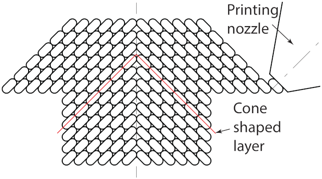
Having a 45° tilted nozzle and a rotational axis around the z-axis enables 90° overhangs without support. In contrast to the conventional FDM printer, where the layers are parallel to the printing plane, the layers become cone shaped with this new system. Figure 1 shows this cone shaped layers and 90° overhangs towards the outside of the part. Printing a given geometry with this kinematics requires a geometry with layers having a cone shape.
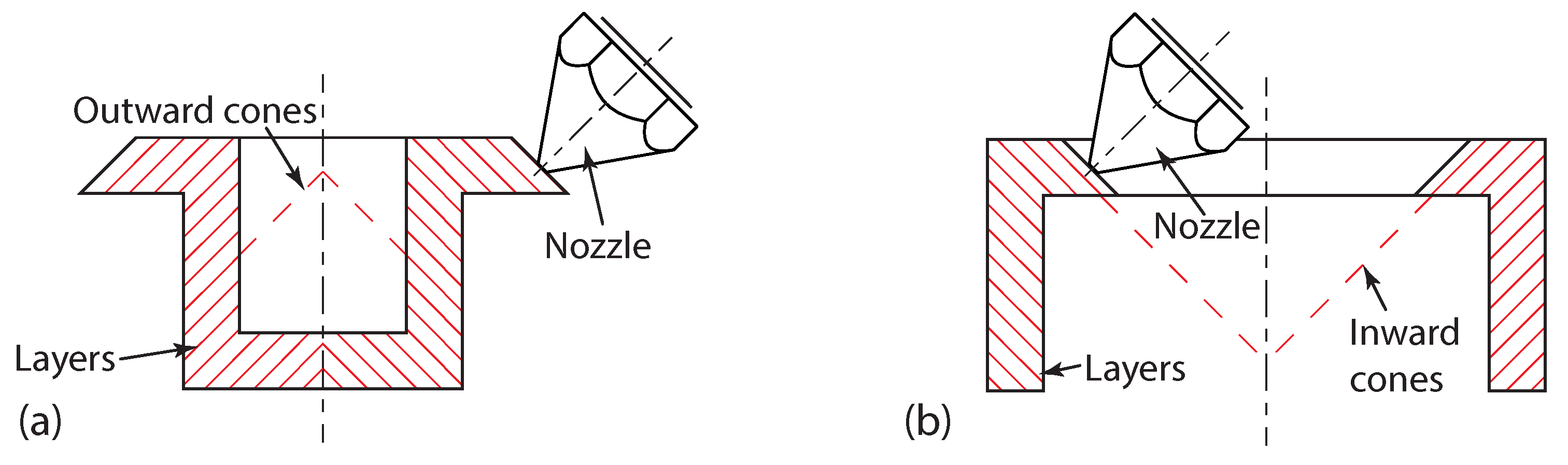
Depending on the direction of the overhangs, the cone is an outward cone for overhangs towards the outside or an inward cone for overhangs towards the inside as shown in Figure 2. The presented slicing strategy only slices parts with overhangs in one direction. Therefore, the possible geometries are limited at the moment. More complicated geometries with overhangs to the outside and overhangs to the inside, can be split into segments with overhangs in only one direction. A theoretical outline of this printing approach is also discussed in [20]. As soon as the splitting up and slicing of individual segments is solved, a big variety of the real-world parts becomes printable without support.
Müller [21] presents on his blog another important result with a conic slicing approach, where conic slicing approach is used to print 90° overhangs with a conventional 3-axis printer. He adapted the conic slicing with a much lower angle (15–25°), such that the non-tilted nozzle does not interfere with the already printed part.
1.3. Conventional Slicing Process
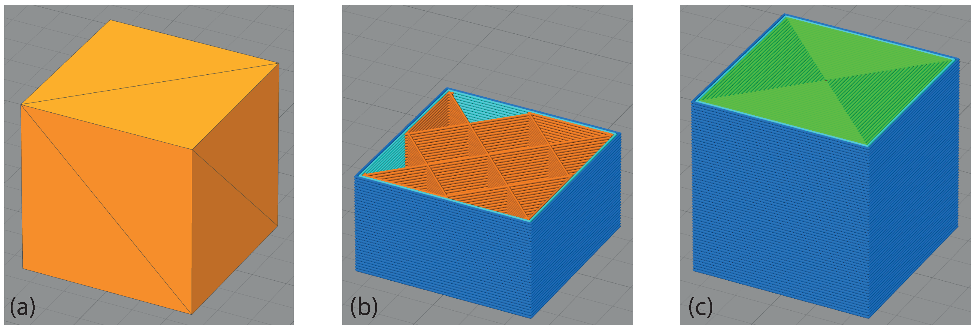
A slicing software, also called “slicer”, transforms the geometry information for a 3D model into printer commands in G-code format to print the part. This geometrical information is stored in an STL file (Standard Tessellation Language). Many different slicing softwares are available on the market (e.g., Simplify3D). An STL part is the input of the slicing process, the G-code the output (Figure 3).
2. A Novel Slicing Strategy with Geometrical Pre- and Post-Transformation
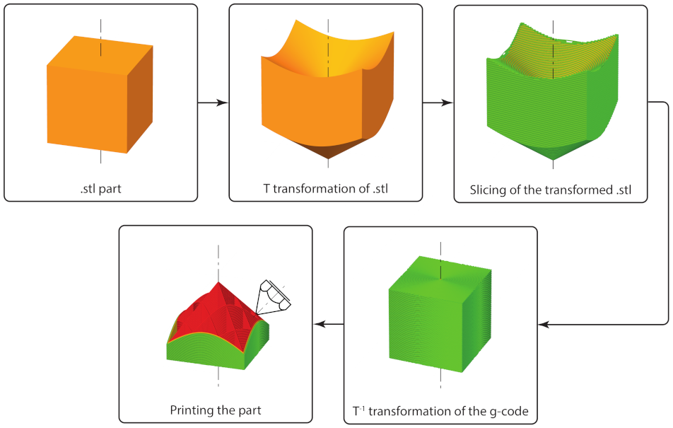
Cone shaped layers are the basis to print a part with the 4-axis printer as described in Figure 1 A novel slicing strategy has been developed for this approach. The novel approach was inspired by the work of Coupek et al. [8], who proposed to geometrically transform the STL file, then slice it with an available slicer and transform it back to the original geometry. This approach has then been adapted to the RotBot kinematics, where Python scripts execute the transformations [22]. The software files can be found on GitHub [23].
2.1. Geometrical Transformation for Cone Shaped Layers
As described in Section 1.3, a conventional slicer divides the model in layers with a fixed z-value. On the other side, the cone shaped layers consist of concentric circles each circle having a different (constant) z-value and a different (constant) radius. The conic layers of circles are transformed in a plane with a constant z-value to slice the part with a conventional slicer. This is done with the transformation T shown in Equation (1)
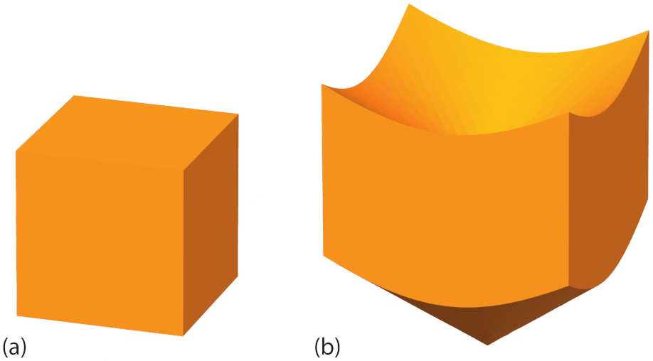
The transformation T is a radial dilation by the factor in the x-y-plane and a radius-dependent translation in the z-direction. Figure 4 shows an example of an original cube and its transformation.
After slicing the geometry, the reverse transformation has a very similar form as T itself and is shown in Equation (2)
is a radial dilatation by in the x-y-plane and again a radius-dependent translation in the z-direction.
Figure 5 illustrates the workflow for the presented slicing strategy. First the STL file is convertedwith the shown transformation T, which is described in more detail in Section 2.2. Then this STL file is sliced with a conventional slicer with optimized settings as described in Section 2.3. After that, the G-code is back-transformed using , which is presented in Section 2.4.
2.2. Pre-Transformation of the STL File
A refinement step reduces the size of the triangles to transform the STL file. These concepts are shown in the following sections.
2.2.1. Refinement of Triangulation
The STL file describes the triangulated surface by the unit normal and the vertices of the triangles in a three-dimensional Cartesian coordinate system. The following shows the definition of one triangle in an ASCII STL file:
facet normal ni nj nk
outer loop
vertex v1x v1y v1z
vertex v2x v2y v2z
vertex v3x v3y v3z
endloop
endfacet
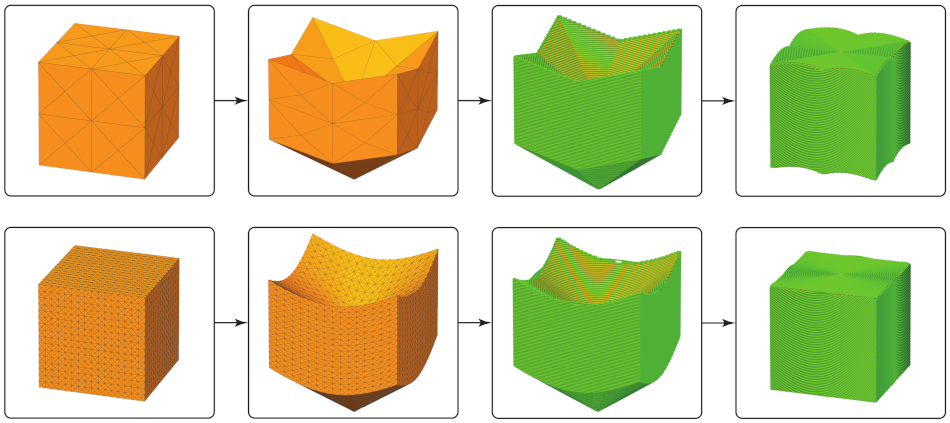
The triangles are usually as large as possible to keep the file size small. However, with this slicing approach, large triangles lead to artifacts, which decrease the surface quality of the printed object dramatically. Figure 6 shows this effect, where the triangles of the upper STL file have a length of 15 mm and the ones of the lower STL have a length of 2 mm. So, the maximal size of the triangles is decreased, until the part reaches the required surface quality. Experience shows that the maximal length of a side of a triangle should be between 1–2 mm.
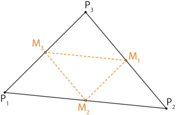
There are different ways to refine the triangles. One is to use the export settings of the CAD, where possibly the maximal triangle size can be defined. Another way is to integrate the refinement into the Python script that transforms the STL file. Therefore, the sides of each triangle are bisected, and the three newly generated midpoints are connected (Figure 7). One triangle produces four smaller (and congruent) triangles with this procedure.
An easy solution is to repeat the refinement several times to all triangles. However, the downside of applying it to all triangles is that already small triangles are unnecessarily refined. This has a negative effect on the file size and the computational time.
2.2.2. Transformation of Triangles and Implementation of the Transformation
The transformation T shown in Equation (1) is executed to all vertices of a triangle by a Python script to transform all the triangles. One possibility to work with STL files in Python is by using the numpy-stl package [24]. It relies heavily on the numpy package and promises to be fast in manipulating STL files. Using this package, a STL file is read and stored as a MESH object. Such an object has different attributes, such as points, which is an array of all points describing the object or normals which is an array of normal vectors of each face of the object. The attribute vector is used, which is an array of triangles describing the object. Then it is proceeded as follows:
- 1.
- Read the STL file and store it as a MESH object.
- 2.
- Extract the array of triangles describing the object using the vector attribute.
- 3.
- Refine the triangulation by applying the refining step a given number of times. If there are N triangles and the refining step is done m times, the output is .
- 4.
- Apply the transformation T to the refined triangulation.
- 5.
- Store the transformed triangulation as a MESH object and save it in a new STL file.
2.3. Slicing in Conventional Slicer
Different parameter settings in the slicing software define the way a part is printed. Important settings with a significant influence on the printing quality are the layer height, the extrusion width, the number of perimeters, which perimeter is printed first (inside or outside), the number of solid bottom and top layers and the internal fill pattern. The following settings turned out to be useful:
- Layer height = mm
- Extrusion width = mm (diameter of the nozzle sets the maximum value)
- Number of perimeters = 2
- Outline Direction = Inside-Out
- Number of solid bottom layers = 0
- Number of solid top layers = 0
- Internal fill pattern = grid
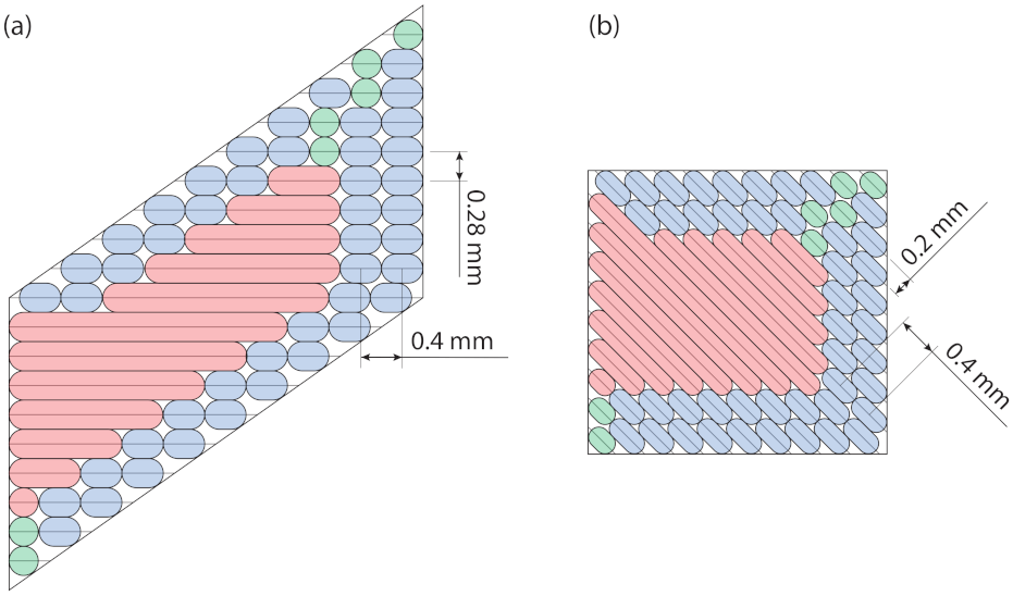
Figure 8 shows a simplified section through a sliced object. The light blue colored strands are the perimeters. If the width of a thin part is not an integer multiple of the extrusion width (thin part width ≠ n × extrusion width), then the slicer generates perimeters with an adjusted width to fill the gaps. These perimeters are shown in a light green color. The infill strands are light red.
In the conventional printer setup, a newly printed strand is always good supported. Therefore, it is flattened and widened during the printing process. Support could miss with the novel printing setup and the strand is therefore sometimes not widened and the extrusion width may not be wider than the diameter of the nozzle to ensure that the strands have a good connection to the already printed part. The back-transformation of the G-code the sliced layer height of mm is reduced to a rectangular distance of the cone shaped layers of mm. The extrusion width of mm remain the same, due to the characteristics of the transformation , where the length in radial direction remains the same. This results in a 2:1 ratio between the extrusion width and the layer height. This ratio gives a good overlap of 50% between the single strands of two different layers. The horizontal bottom and top layers are sliced as perimeters. This is the reason why no solid top and bottom layers are required. Depending on the geometry of the part, this setting will have to be adjusted.
Since the material flow is adjusted while transforming the G-code back with as explained in Section 2.4.4, the slicer has to be set to relative extrusion.
2.4. Back-Transformation of G-Code
Transforming the G-code back with to its original geometrical dimensions is more complicated than transforming the STL file with T, since different values have to be determined. The following steps are required to transform the G-code back:
- 1.
- Splitting long elements into short segments
- 2.
- Transforming x, y and z
- 3.
- Adjusting the extrusion amount
- 4.
- Calculating the required angle of the rotational axis
- 5.
- Writing the new G-code
2.4.1. General Back-Transformation
The transformation refers to all coordinates of the G-code (2). The G-code basically is a set of moving instructionsfor the printhead, where each moving command only defines the endpoint of where the printhead will move to. So, there the position of the printhead before the execution of the instruction, which is defined as the “old” point, and the position of the printhead after the execution, which is defined as the “new” point. After every moving step, the “new” point becomes the new “old” point. There are the following relevant values for the back-transformation, where the back-transformed values are marked with “bt”:
- Coordinates of “old” point:
- “Old” coordinates back-transformed:
- Coordinates of “new” point:
- “New” coordinates back-transformed:
- z-coordinate of current layer:
2.4.2. Splitting Long Elements
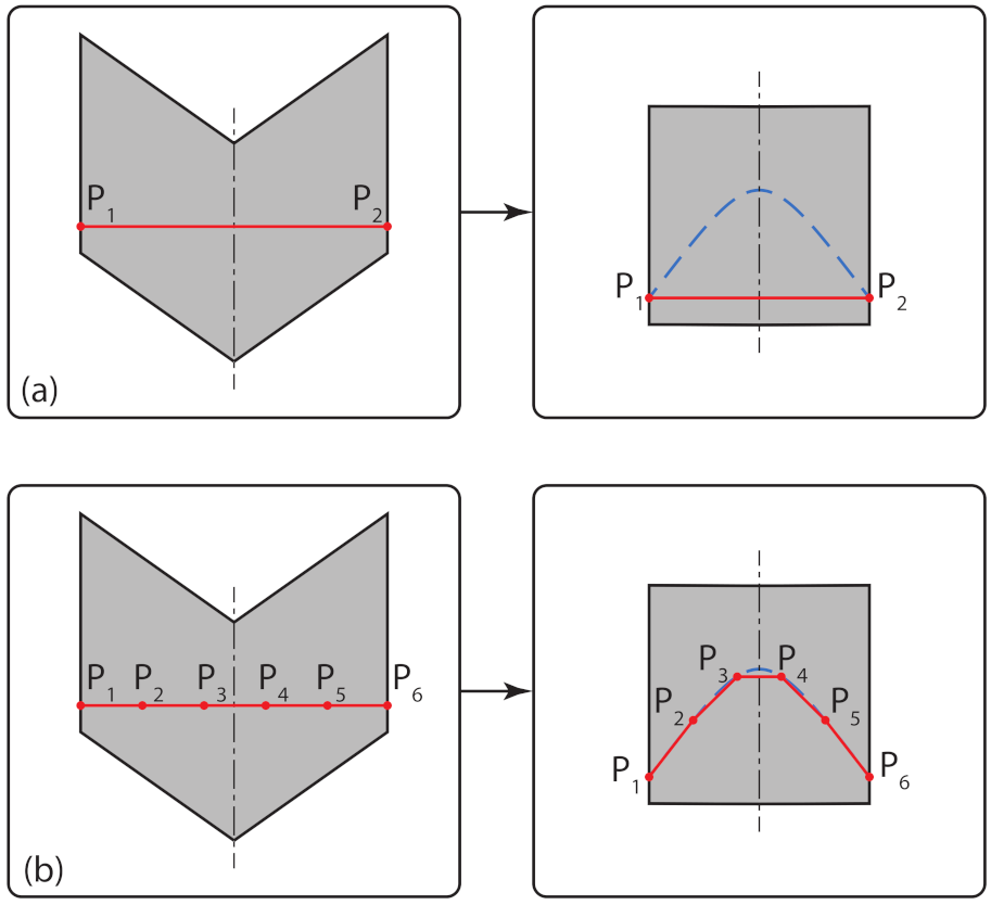
Since does not transform lines into linear lines, long line segments may have to be split. The upper left drawing of Figure 9 shows a linear move, which can be described with one G-code command. The nozzle would be in position (“old” point) and the endpoint of the line would be in (“new” point). When this line consisting of the start-point and the end-point, now is back-transformed with , then the printer would follow a line, again from to (upper right drawing). However, with an infinitesimal transformation , the nozzle would have to move on a cone section, here a hyperbolic curve, shown in blue. Lines have to be split into small segments of equal length to achieve proper accuracy. Thereby, the segments must be be short enough to achieve the required accuracy. However, too short segments increase the size of the G-code file.
The length of the element is computed with Equation (3) to evaluate the required number of elements:
2.4.3. Transforming x, y and z
This leads to the - and z-values (Since the values are already back-transformed, the factor can be omitted in the formula for .). Each movement command becomes a vector of movement commands due to the split elements in the back-transformed G-code. The equations corresponding are given in Appendix A.1.
2.4.4. Adjustment of Material Flow
The characteristics of the transformation causes that lengths in radial direction remain the same and lengths perpendicular to the radial direction are divided by . Since the amount of extruded material is a function of the length of an element, a new evaluation of the material flow is needed while transforming the G-code back. This is done by comparing the length of the element before and after the transformation, so that the amount of extruded material per length stays constant. Additionally, the extrusion is divided by , since the layer height is reduced by the same factor (see Section 2.3). The equations to calculate the amount of extruded plastic is in Appendix A.2.
2.4.5. Calculation of the Nozzle Orientation
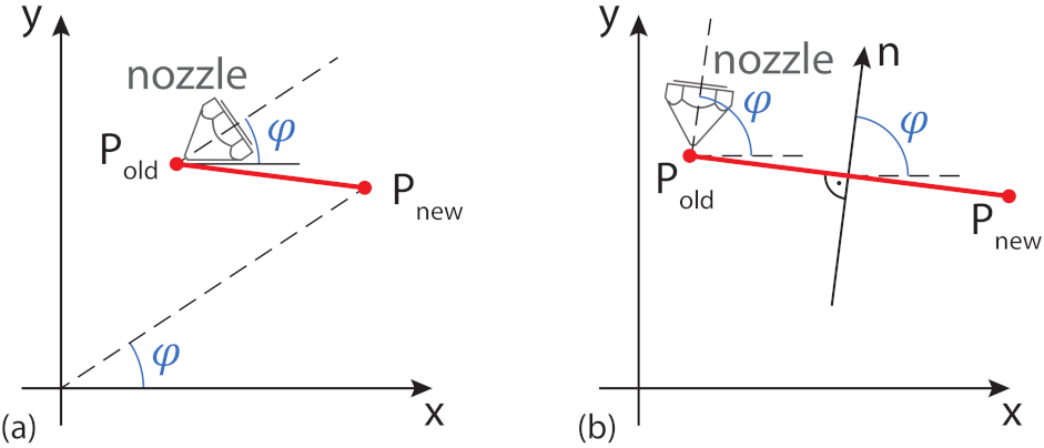
The slicing software determines the x-, y- and z-coordinates and the necessary material flow. The orientation of the nozzle around the rotational z-axis has to be calculated within the back-transformation. Since the rotation is around the z-axis, the orientation of the nozzle is independent of the z-value and only depends on the x- and y-values. Two different approaches are suitable:
- Radial orientation: The nozzle is always oriented towards the origin of the coordinate system, no matter in what direction it moves.
- Tangential orientation: The nozzle is always perpendicular to the movement in the x- and y-plane.
Both methods have their advantages and disadvantages. However, the radial orientation has turned out to be the simpler solution with no remarkable downsides on the quality.
Radial orientation:
The simpler way to compute the radial angle is to take the “new” point and to calculate its polar angle in the x-y-plane and set the nozzle orientation to this angle (Figure 10a). Since longer elements are split into short segments, alignment to the “new” point is sufficient and there is no need to adjust the angle while moving in one segment. This leads to the nozzle orientation towards the origin and therefore also to the center axis of the cone. So, no collision with the printhead and the already printed part can occur. One downside of this method is the nonideal orientation of the nozzle with respect to the material flow.
Tangential orientation: For the tangential orientation of the nozzle, the normal to the line of movement has to be calculated. Thereby, the normal pointing away from the origin is chosen (Figure 10b) to prevent the printhead of colliding with the already printed material. The major downside of this method is the increase of printing head rotation for small linear movements in different directions.
2.4.6. Calculating the Rotational G-Code Values
Depending on the printer firmware, different designations for the orientation are common. A Duet3D controller with RepRap Firmware was used in this project, where the rotational axis is defined as the U-axis. So, the information about the rotation of the nozzle is added as the U-value in the G-code. The computed angle cannot be directly used as U-value:
- The units of the computed angle must be in degrees, so conversion may be required.
- The values of the angles are between . When crossing the x-axis for , this would lead the U-value to have “large, discontinuous” jumps.
An array of angle values () is used to prevent the angle from these discontinuous changes. Starting form , is successively chosen:
From all 21 possible angles , the angle closest to is predecessor is chosen. Then only the m values are used to compute the U-values
By definition of , values in the range or equivalently are used, which can be exceeded, when the printing head is rotated many times. The U-value is reset by using a command in the G-code, whenever a is used to assure that the values remain in .
If , the following line is inserted:
Additional line:
2.4.7. Writing the New Code
After the execution of the back-transformation, the new G-code is written:
Original G-code line:
Back-transformed G-code:
2.5. Inward Cone: Slicing for Inward Overhangs
As mentioned in Section 1.2, depending on the direction of the overhang outward or inward cone shaped layers are used. All the above-mentioned concepts of the novel slicing strategy are demonstrated with outward cones (Figure 2a). All these concepts can be adopted for the use with inward cones (Figure 2b). The only difference in the transformation T and for the inward cone is in the calculation of the z-value (Equations (5) and (6)), where the z correction term, depending on the x- and y- value, now have a opposite sign.
The basic concept of the back-transformation and all steps included stay the same. The hyperbolic curves for the movement of the nozzle now are all directed downwards. This can lead to collisions with already extruded material or the printing platform. Therefore, an additional criterion is introduced. Whenever:
- an inward cone is used for the transformation and
- no material is extruded and
- the nozzle is moved in x- and/or y-direction
the nozzle has to move linear from the “old” point to the “new” point (instead of moving along a hyperbolic arc).
3. Results
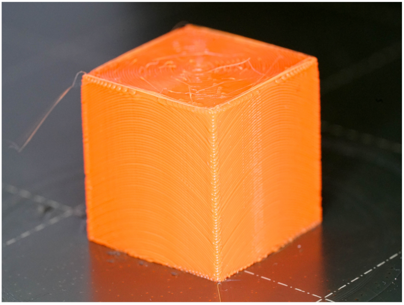
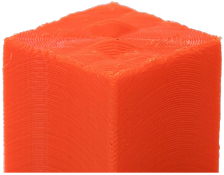
Cubes with no overhangs have been printed to evaluate the slicing strategy. Figure 11 shows the cone shaped layer of a cube with a radial orientation of the nozzle and Figure 12 the finished cube with the strands on the surface following a hyperbolic curve. The picture indicates a reasonable quality with this slicing approach. Nevertheless, the surface quality is not yet at the level of parts printed on x-y-z printers due to the lack of optimization of the slicing software for a 4-axis kinematics.
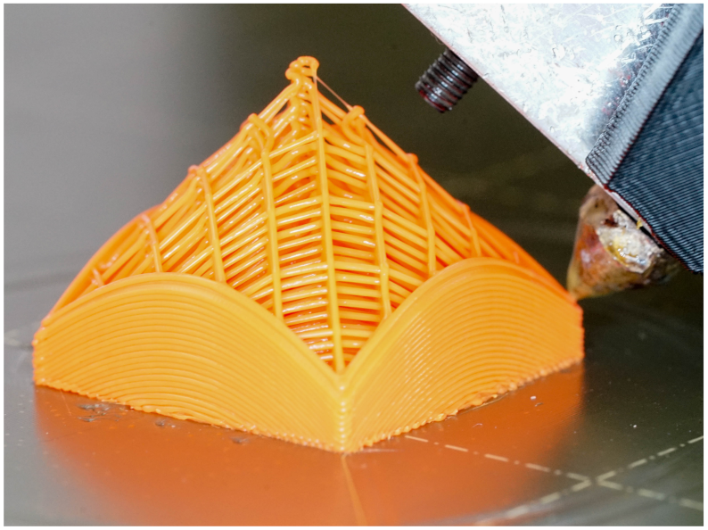
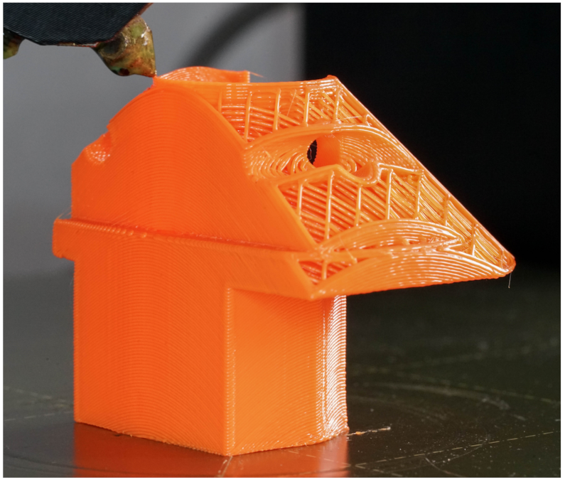
Figure 13 shows the top surface of a cube with artifacts, due to too big triangles in the STL file, as described in Section 2.2.1. The slicing strategy also proved to work unproblematically for more complicated parts with 90° overhangs and holes. Figure 14 shows such a part being printed with the nozzle oriented in radial direction.
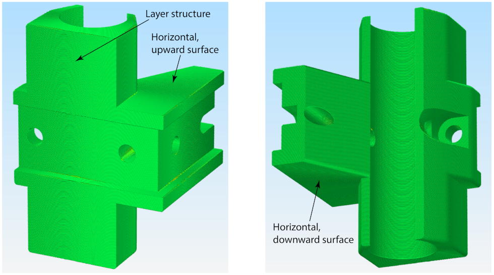
Several papers investigate the impact of different parameters on the dimensional accuracy and the surface roughness of FDM printed parts ([7,25,26,27,28,29,30]. To date, no fully comprehensive series of measurements have been conducted with the novel slicing strategy presented regarding the various influencing parameters. With a limited number of tests, a set of reasonable printing parameters could be found (Section 2.3). A reference geometry (Figure 15) has been printed with these settings on the RotBot and with corresponding settings on a Prusa Mk3s to compare the geometrical accuracy and the surface roughness (Table 1).
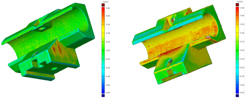
For a quantitative comparison, the parts have been 3D scanned with a HandySCAN 3D scanner and evaluated with the VXElements software from Creaform. The scanning accuracy has been set to a maximum of m. The measured geometry shape has then been compared with the CAD geometry, using the software Gom Inspect.
Figure 16 shows the deviation from the scanned parts and the CAD file. The part printed on the Prusa (left) has a deviation between approximately and mm. Downward overhangs have the biggest offset with a deviation of up to mm. The part printed on the RotBot (right) has a higher deviation of about to mm. The maximum offset in this part can be found on the edges. The reduction of the material flow and an adjusted calibration of the nozzle could help to reduce the offset.
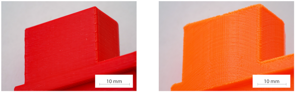
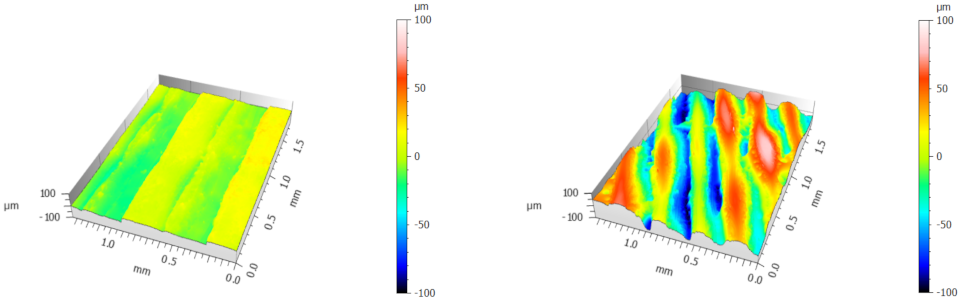
3 different surfaces (marked in Figure 15) of the two reference parts have been scanned with a confocal z scan (m) on a Leica DCM 3D microscope with an EPI 20X-L objective to quantify the surface ripple and in particularly its roughness. 9 individual surface scans have been stitched together to reach a representative area with the high magnification. This leads to surfaces of about mm. This surface scans, all with the same color scale, and close up pictures showing the same surfaces for a visual evaluation of the quality are printed in Figure 17, Figure 18, Figure 19, Figure 20, Figure 21 and Figure 22.
Figure 17 displays the parallel layers of the part printed on the Prusa and the conical shaped layers of the part printed on the RotBot. The Prusa printer shows a higher regularity to the eye.
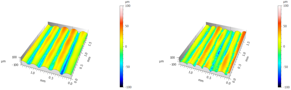
Figure 18 illustrates the ripple and the roughness of the vertical surfaces with the horizontal layers. The measured values are shown in Table 2. It reveals that both reference parts have very similar values.
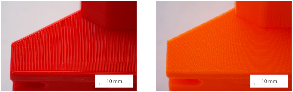
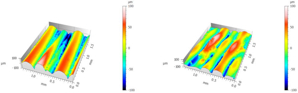
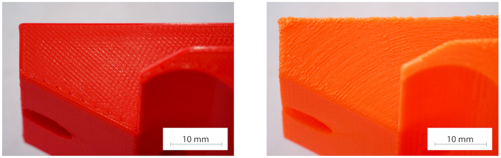
The Figure 19 and Figure 21 provide a closeup of the surface of upward and downward horizontal planes. While the Prusa printer produces a noticeable difference between an upward and a supported downward surface, almost no difference is visible on the pictures of the RotBot. The downward surface seems to be of better quality.
The measured values of the scans prove this assumption (Table 2). The upward surface of the Prusa part shows very low roughness, where the the values of the downward surface are significantly higher. The RotBot part has very similar results for the upward as for the downward surface.
The vertical surfaces are of a comparable quality. The RotBot printer produces upward and unsupported downward surfaces of comparable quality. The difference of the upward and the supported downward surface is significant for a conventional x-y-z printer.
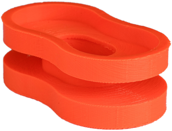
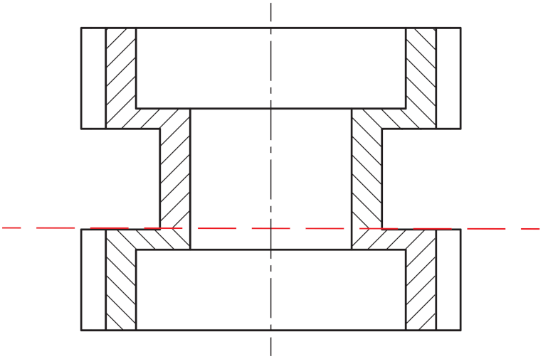
A part with a combination of an inside and an outside overhang is shown in Figure 23. Therefore, the part was split up in two parts, a lower part with the inward overhang and an upper part with the outside overhang. These parts have been sliced separately with an inward cone for the lower part and an outward cone for the upper part. After transforming the G-code back, the two parts have been combined by simply adding the two G-codes. Figure 24 illustrates the section through the part with the cutting line (red), the inward cone in the lower part and the outward cone in the upper part.
4. Discussion
Section 3 proofs, that the approach works in general but that the quality is not yet on the level of conventionally produced FDM parts. One reason for this is that conventional slicing software is optimized for the x-y-z kinematics. For example, a top layer is treated differently by the slicer than a perimeter. Transforming the G-code back, a perimeter can become a top layer and vice versa. Further research and testing for the slicer settings is required to improve the quality of the prints. At the moment it is not possible to distinguish whether it is mainly the hardware or the slicing strategy that causes the main quality losses.
Beside the quality issues, there are other topics worthy of further investigation:
- The refinement of the triangles is done with a very simple approach. This leads to unoptimized STL files. The refinement should be done in a way, that only the bigger triangles are refined until all triangles are small enough to fulfill the requirements. To keep the number of triangles low, the already small triangles must not be affected.
- As stated in Section 3, the movement of the RotBot needs further improvement. The optimal speeds, accelerations and jerks of the different axes have to be optimized for the reduction of the printing time and constant printing quality.
- As described in Section 1.2, more complicated geometries with a combination of overhangs to the inside and the outside direction must be separated and sliced independently. Up to now, this only has been done manually with very simple combinations as shown in Section 3. Further research and testing have to be done to manage a variety of different geometries, with the aim of an automated analysis and separation.
- Parts that can be sliced with only one outward transformation do not have any collision problem, since the printhead always is on the outside of the cone. However, parts with inward cones and parts with a combination of different cones do face collision problems. This has be investigated further and solutions have to be developed.
- The Python file for the back-transformation is optimized to work with G-codes from one defined slicer (Simplify3D). Other slicers could include commands into the G-code that are not handled correctly with the Python script. One example are the comment lines, which are used in the back-transformation script to differentiate between infill and perimeter. Therefore, a more generic Python script has to be written.
- It should also be considered to develop a completely new slicer software optimized for the conical layers. This would prevent the geometric transformation and reverse transformation and the slicing with a conventional slicer. Despite the enormous development effort, certain problems could be handled more directly in this way. For example, the refinement of the triangles or the splitting of the straight lines would be omitted. The quality problems could also be solved more easily since the slicer would be optimized for the conical layers.
Beside the work of Müller [21], there is no other work known, where a similar slicing strategy was used or tested on an other machine than the 4-axis printer RotBot. At the moment there are no plans to test it on an other kinematics. The work of Coupek et al. [8] shows, that comparable approaches could be a feasible solution for other problems in the field of 3Dp.
Since professional FDM printers often work with soluble supports, the presented slicing and printing approach could therefore mainly be interesting for the group of printers, using the same material for the part and the support structure. If the remaining challenges can be solved, the outcome will be a enormous reduction of support material. However, there are major difficulties, like the automated splitting up of complicated parts, which must be solved to advance the whole process.
5. Conclusions
New 3D printer kinematics require adapted slicing strategies and algorithms for adequate path planning. An algorithm with a geometrical transformation of the generated STL file, followed by a conventional slicing process and a back-transformation of the G-code is presented in this paper. Analysis of two printed reference parts led to the following observations:
- The study demonstrates that the novel slicing strategy with cone shaped layers works very well on the 4-axis printer.
- It is possible to print parts with 90° overhangs without the use of support material. The downward oriented surfaces have the same quality as the upward oriented surfaces.
- The accuracy of the printed part geometry and the surface roughness as well are not yet as good compared to a conventional 3D printer with orthogonal kinematics.
The motivation for this work was the development of a system capable of printing parts with large overhangs without support material. The outcomes of this R&D prove the feasibility of the chosen approach.
Author Contributions
Conceptualization, M.W., M.G. and W.J.E.; methodology, M.W. and M.G.; software, M.G.; validation, W.J.E. and M.W.; investigation, M.W.; resources, M.W.; writing—original draft preparation, M.W.; writing—review and editing, W.J.E., M.G. and C.J.; visualization, M.W., W.J.E. and M.G.; supervision, W.J.E. and M.W. All authors have read and agreed to the published version of the manuscript.
Funding
This research received no external funding.
Institutional Review Board Statement
Not applicable.
Informed Consent Statement
Not applicable.
Data Availability Statement
Not applicable.
Conflicts of Interest
The authors declare no conflict of interest.
Abbreviations
The following abbreviations are used in this manuscript:
| 3Dp | 3D printing |
| AM | Additive manufacturing |
| FDM | Fused Deposition Modeling |
| CNC | Computer Numeric Control |
| DED | Direct Energy Deposition (aka DMD) |
| ZHAW | Zurich University of Applied Sciences |
| STL | Standard Tessellation Language |
Appendix A
Appendix A.1
Equations to calculate the movement vectors for the G-code described in Section 2.4.3:
Appendix A.2
The extruder flow () in a back-transformed element is calculated as follows (see Section 2.4.4):
where d is the distance, defined in Equation (3) and e is the extruded amount of material in the original line.
References
- Wong, K.V.; Hernandez, A. A Review of Additive Manufacturing. ISRN Mech. Eng. 2012, 2012, 1–10. [Google Scholar] [CrossRef] [Green Version]
- Thompson, M.K.; Moroni, G.; Vaneker, T.; Fadel, G.; Campbell, R.I.; Gibson, I.; Bernard, A.; Schulz, J.; Graf, P.; Ahuja, B.; et al. Design for Additive Manufacturing: Trends, opportunities, considerations, and constraints. CIRP Ann. 2016, 65, 737–760. [Google Scholar] [CrossRef] [Green Version]
- Rahim, T.N.A.T.; Abdullah, A.M.; Akil, H.M. Recent Developments in Fused Deposition Modeling-Based 3D Printing of Polymers and Their Composites. Polym. Rev. 2019, 59, 589–624. [Google Scholar] [CrossRef]
- Wulle, F.; Coupek, D.; Schäffner, F.; Verl, A.; Oberhofer, F.; Maier, T. Workpiece and Machine Design in Additive Manufacturing for Multi-Axis Fused Deposition Modeling. Procedia CIRP 2017, 60, 229–234. [Google Scholar] [CrossRef]
- Verbeeten, W.M.; Lorenzo-Bañuelos, M.; Arribas-Subiñas, P.J. Anisotropic rate-dependent mechanical behavior of Poly(Lactic Acid) processed by Material Extrusion Additive Manufacturing. Addit. Manuf. 2020, 31, 100968. [Google Scholar] [CrossRef]
- Jiang, J.; Xu, X.; Stringer, J. Support Structures for Additive Manufacturing: A Review. J. Manuf. Mater. Process. 2018, 2, 64. [Google Scholar] [CrossRef] [Green Version]
- Volpato, N.; Foggiatto, J.A.; Schwarz, D.C. The influence of support base on FDM accuracy in Z. Rapid Prototyp. J. 2014, 20, 182–191. [Google Scholar] [CrossRef]
- Coupek, D.; Friedrich, J.; Battran, D.; Riedel, O. Reduction of Support Structures and Building Time by Optimized Path Planning Algorithms in Multi-axis Additive Manufacturing. Procedia CIRP 2018, 67, 221–226. [Google Scholar] [CrossRef]
- Reeser, K.; Doiron, A.L. Three-Dimensional Printing on a Rotating Cylindrical Mandrel: A Review of Additive-Lathe 3D Printing Technology. 3D Print. Addit. Manuf. 2019, 6, 293–307. [Google Scholar] [CrossRef]
- Park, H.S.; Park, H.J.; Lee, J.; Kim, P.; Lee, J.S.; Lee, Y.J.; Seo, Y.B.; Kim, D.Y.; Ajiteru, O.; Lee, O.J.; et al. A 4-Axis Technique for Three-Dimensional Printing of an Artificial Trachea. Tissue Eng. Regen. Med. 2018, 15, 415–425. [Google Scholar] [CrossRef] [PubMed]
- Xu, K.; Chen, L.; Tang, K. Support-Free Layered Process Planning Toward 3+2-Axis Additive Manufacturing. IEEE Trans. Autom. Sci. Eng. 2019, 16, 838–850. [Google Scholar] [CrossRef]
- Murtezaoglu, Y.; Plakhotnik, D.; Stautner, M.; Vaneker, T.; van Houten, F.J. Geometry-Based Process Planning for Multi-Axis Support-Free Additive Manufacturing. Procedia CIRP 2018, 78, 73–78. [Google Scholar] [CrossRef]
- Lee, K.; Jee, H. Slicing algorithms for multi-axis 3-D metal printing of overhangs. J. Mech. Sci. Technol. 2015, 29, 5139–5144. [Google Scholar] [CrossRef]
- Sundaram, R.; Choi, J. A Slicing Procedure for 5-Axis LaserAided DMD Process. J. Manuf. Sci. Eng. 2004, 126, 632–636. [Google Scholar] [CrossRef]
- Wang, M.; Zhang, H.; Hu, Q.; Liu, D.; Lammer, H. Research and implementation of a non-supporting 3D printing method based on 5-axis dynamic slice algorithm. Robot. Comput.-Integr. Manuf. 2019, 57, 496–505. [Google Scholar] [CrossRef]
- Wu, C.; Dai, C.; Fang, G.; Liu, Y.J.; Wang, C.C. RoboFDM: A robotic system for support-free fabrication using FDM. In Proceedings of the 2017 IEEE International Conference on Robotics and Automation (ICRA), Singapore, 29 May–3 June 2017; IEEE: Piscataway, NJ, USA, 2017. [Google Scholar] [CrossRef]
- Ishak, I.B.; Fisher, J.; Larochelle, P. Robot Arm Platform for Additive Manufacturing Using Multi-Plane Toolpaths. In Proceedings of the Volume 5A: 40th Mechanisms and Robotics Conference; Charlotte, NC, USA, 21–24 August 2016, American Society of Mechanical Engineers: New York, NY, USA, 2016. [Google Scholar] [CrossRef] [Green Version]
- Zhao, G.; Ma, G.; Feng, J.; Xiao, W. Nonplanar slicing and path generation methods for robotic additive manufacturing. Int. J. Adv. Manuf. Technol. 2018, 96, 3149–3159. [Google Scholar] [CrossRef]
- Herrman, D.; Tolar, O. Weiterentwicklung der Gerätetechnik im FDM-Verfahren. Master’s Thesis, ZHAW, Winterthur, Switzerland, 2015. [Google Scholar]
- Wüthrich, M.; Elspass, W.J.; Bos, P.; Holdener, S. Novel 4-Axis 3D Printing Process to Print Overhangs Without Support Material. In Industrializing Additive Manufacturing; Meboldt, M., Klahn, C., Eds.; Springer International Publishing: Cham, Switzerland, 2021; pp. 130–145. [Google Scholar] [CrossRef]
- XYZdims.com. Available online: https://xyzdims.com/2021/03/03/3d-printing-90-overhangs-without-support-structure-with-non-planar-slicing-on-3-axis-printer/ (accessed on 19 July 2021).
- Gubser, M. FDM Printing of Overhangs without Support Material. Master’s Thesis, ZHAW, Winterthur, Switzerland, 2020. [Google Scholar]
- GitHub Software. Available online: https://github.com/RotBotSlicer/Transform (accessed on 18 August 2021).
- Numpy-STL Documentation. Available online: https://numpy-stl.readthedocs.io/en/latest/index.html (accessed on 19 July 2021).
- Turner, B.N.; Gold, S.A. A review of melt extrusion additive manufacturing processes: II. Materials, dimensional accuracy, and surface roughness. Rapid Prototyp. J. 2015, 21, 250–261. [Google Scholar] [CrossRef]
- Mohamed, O.A.; Masood, S.H.; Bhowmik, J.L. Optimization of fused deposition modeling process parameters: A review of current research and future prospects. Adv. Manuf. 2015, 3, 42–53. [Google Scholar] [CrossRef]
- Dey, A.; Yodo, N. A Systematic Survey of FDM Process Parameter Optimization and Their Influence on Part Characteristics. J. Manuf. Mater. Process. 2019, 3, 64. [Google Scholar] [CrossRef] [Green Version]
- Turek, P.; Budzik, G. Estimating the Accuracy of Mandible Anatomical Models Manufactured Using Material Extrusion Methods. Polymers 2021, 13, 2271. [Google Scholar] [CrossRef]
- Nancharaiah, T.; Raju, D.R.; Raju, V.R. An experimental investigation on surface quality and dimensional accuracy of FDM components. Int. J. Emerg. Technol. 2010, 1, 106–111. [Google Scholar]
- Polak, R.; Sedlacek, F.; Raz, K. Determination of FDM Printer Settings with Regard to Geometrical Accuracy. In DAAAM Proceedings; DAAAM International Vienna: Vienna, Austria, 2017; pp. 0561–0566. [Google Scholar] [CrossRef]
Figure 1.
Printing strategy with the cone shaped layers.

Figure 2.
Depending on the direction of the overhangs, a different cone has to be chosen: (a) An outward cone for parts with overhangs towards the outside and (b) an inward cone for overhangs towards the inside.
Figure 2.
Depending on the direction of the overhangs, a different cone has to be chosen: (a) An outward cone for parts with overhangs towards the outside and (b) an inward cone for overhangs towards the inside.

Figure 3.
The surface of the geometry is defined with triangles (a) in the STL file. The slicer then converts this surface information into a solid geometry and splits the geometry into slices (layers) with an equal layer height and generates the path for the printer according to the settings. The layer consists at least of the outline of the part (so called perimeter) and the infill. Figure (b) shows the outer (blue) and the inner (light blue) perimeter and the 10% infill (orange) of the layers. The lowest and the most upper layers are printed solid to close the part (green surface in Figure (c)).

Figure 4.
Visualization of the Transformation T with a cube. (a) shows the original cube, whereas (b) shows the transformed geometry in the same scale.
Figure 4.
Visualization of the Transformation T with a cube. (a) shows the original cube, whereas (b) shows the transformed geometry in the same scale.

Figure 5.
Workflow architecture of the slicing strategy.

Figure 6.
Difference of transformation according to the size of the triangles.

Figure 7.
Refinement of the triangles by bisecting its sides.

Figure 8.
Section through a sliced object (simplified). The sliced part in the transformed state (a) and the part after the G-code is transformed with (b).
Figure 8.
Section through a sliced object (simplified). The sliced part in the transformed state (a) and the part after the G-code is transformed with (b).

Figure 9.
Splitting of elements to achieve proper accuracy. In (a) long elements are not split, while in (b) the element is split in 5 segments.
Figure 9.
Splitting of elements to achieve proper accuracy. In (a) long elements are not split, while in (b) the element is split in 5 segments.

Figure 10.
Orientation of the nozzle: (a) Nozzle with a radial orientation towards the origin and (b) Nozzle with a tangential orientation according to direction of movement.
Figure 10.
Orientation of the nozzle: (a) Nozzle with a radial orientation towards the origin and (b) Nozzle with a tangential orientation according to direction of movement.

Figure 11.
Printing a cube with a radial orientation of the nozzle.

Figure 12.
Finished cube, with a radial oriented nozzle.

Figure 13.
Top surface with artifacts, due to large triangles.

Figure 14.
Part with outside overhang and holes being printed.

Figure 15.
Conical sliced reference part in Simplify3D preview with the areas investigated marked.

Figure 16.
Shape deviation (CAD vs. print) on Prusa (left) and RotBot (right).

Figure 17.
Horizontal layers of the printed reference part printed on a Prusa Mk3s (red) and the RotBot (orange).
Figure 17.
Horizontal layers of the printed reference part printed on a Prusa Mk3s (red) and the RotBot (orange).

Figure 18.
Roughness scan of vertical surface of reference parts. Prusa (left) and RotBot (right).

Figure 19.
Horizontal, downward 90° overhang printed on a Prusa Mk3s (red, with support) and the RotBot (orange, without support).
Figure 19.
Horizontal, downward 90° overhang printed on a Prusa Mk3s (red, with support) and the RotBot (orange, without support).

Figure 20.
Roughness scans of the horizontal, downward 90° overhang. Prusa (left) and RotBot (right).
Figure 20.
Roughness scans of the horizontal, downward 90° overhang. Prusa (left) and RotBot (right).

Figure 21.
Horizontal, upward 90° surface printed on a Prusa Mk3s (red) and the RotBot (orange).

Figure 22.
Roughness scans of the horizontal, upward surface. Prusa (left) and RotBot (right).

Figure 23.
Part with a combination of inward and outside overhang.

Figure 24.
Section of part with inward and outside overhang.


Table 1.
Comparison of printer settings for reference prints.
| Parameter | Prusa Mk3s | RotBot |
|---|---|---|
| Material | Prusament PLA (red) | Prusament PLA (orange) |
| Support | yes | no |
| Layer height | 0.3 mm | 0.3 mm |
| Infill | 20% | 20% |
| Printing speed (outer perimeter) | 2100 mm/s | 2520 mm/s |
| Printing time | 2 h 54 min | 3 h 58 min 1 |
1 Axis speeds and accelerations of RotBot have not yet been optimized.
Table 2.
Values of surface scan.
| Surface | Ripple, min [μm] | Ripple, max [μm] | Sa [μm] |
|---|---|---|---|
| Vertical surface Prusa | −63.5 | +49.8 | 21.4 |
| Vertical surface RotBot | −64.8 | +47.6 | 20.7 |
| Upward surface Prusa | −23.8 | +22.1 | 8.3 |
| Upward surface RotBot | −99.0 | +94.8 | 33.1 |
| Downward surface Prusa | −129.9 | +72.1 | 37.8 |
| Downward surface RotBot | −98.6 | +85.9 | 29.9 |
Publisher’s Note: MDPI stays neutral with regard to jurisdictional claims in published maps and institutional affiliations. |
© 2021 by the authors. Licensee MDPI, Basel, Switzerland. This article is an open access article distributed under the terms and conditions of the Creative Commons Attribution (CC BY) license (https://creativecommons.org/licenses/by/4.0/).
Share and Cite
MDPI and ACS Style
Wüthrich, M.; Gubser, M.; Elspass, W.J.; Jaeger, C. A Novel Slicing Strategy to Print Overhangs without Support Material. Appl. Sci. 2021, 11, 8760. https://0-doi-org.brum.beds.ac.uk/10.3390/app11188760
AMA Style
Wüthrich M, Gubser M, Elspass WJ, Jaeger C. A Novel Slicing Strategy to Print Overhangs without Support Material. Applied Sciences. 2021; 11(18):8760. https://0-doi-org.brum.beds.ac.uk/10.3390/app11188760
Chicago/Turabian StyleWüthrich, Michael, Maurus Gubser, Wilfried J. Elspass, and Christian Jaeger. 2021. "A Novel Slicing Strategy to Print Overhangs without Support Material" Applied Sciences 11, no. 18: 8760. https://0-doi-org.brum.beds.ac.uk/10.3390/app11188760
Note that from the first issue of 2016, this journal uses article numbers instead of page numbers. See further details here.