
Comparison of Optimal Control Designs for a 5 MW Wind Turbine


1
School of Electronic and Electrical Engineering, Kyungpook National University, Daegu 41566, Korea
2
School of Electronics Engineering, Kyungpook National University, Daegu 41566, Korea
*
Author to whom correspondence should be addressed.
Appl. Sci. 2021, 11(18), 8774; https://0-doi-org.brum.beds.ac.uk/10.3390/app11188774
Submission received: 20 August 2021
/
Revised: 10 September 2021
/
Accepted: 16 September 2021
/
Published: 21 September 2021
(This article belongs to the Special Issue Boosting Wind Power Integration)
Abstract
:Optimal controllers, namely Model Predictive Control (MPC), Control (), and Linear Quadratic Gaussian control (LQG), are designed for a 5 MW horizontal-axis variable-speed wind turbine. The control design models required as part of the optimal control design are obtained by using a high fidelity aeroelastic model (i.e., DNV Bladed). The optimal controllers are eventually designed in three operating modes: below-rated, just below-rated, and above rated-wind speeds, based on linearized control design models. The linearized models are reduced by using a model reduction technique to facilitate the design of optimal controllers. The controllers are analyzed not only in the time domain but also in the frequency domain and on the torque/speed plane. Simulation results demonstrated that optimal controllers perform better than the standard proportional-integral-derivative (PID) controller, particularly for removing oscillation due to the drive-train mode without incorporating a drive-train damper.
1. Introduction
Electricity generation from wind turbines has been one of the most rapidly growing sustainable energy sources in the last decade, with more than 743 GW installed worldwide at the end of 2021, as reported by the Global Wind Energy Council [1], since it does not produce atmospheric emissions. However, generating electricity from wind can be challenging due to various reasons, including operation and maintenance (O&M) costs. Recently, reducing O&M costs, which includes control and condition monitoring and improving reliability, has become crucial in wind turbine and farm operational strategies because of their long-term impact on the reliability and productivity of wind site operations.
The rotor, which consists of nacelle situated on top of the tower, hub, and blades, is a crucial component of the wind turbine (Figure 1). As minimum (cut-in) wind blows toward the blades of the wind turbine generator, it starts increasing speed.
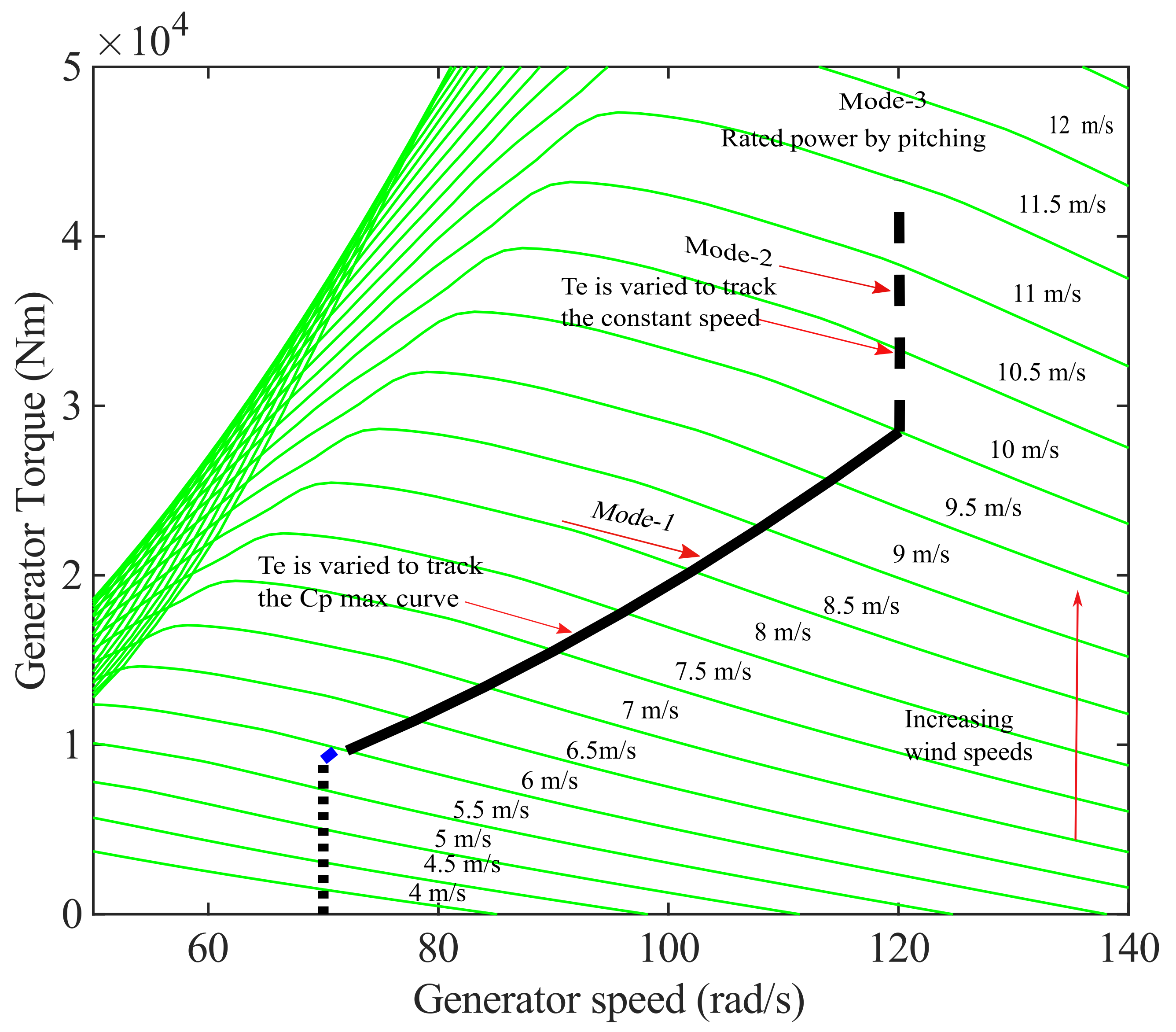
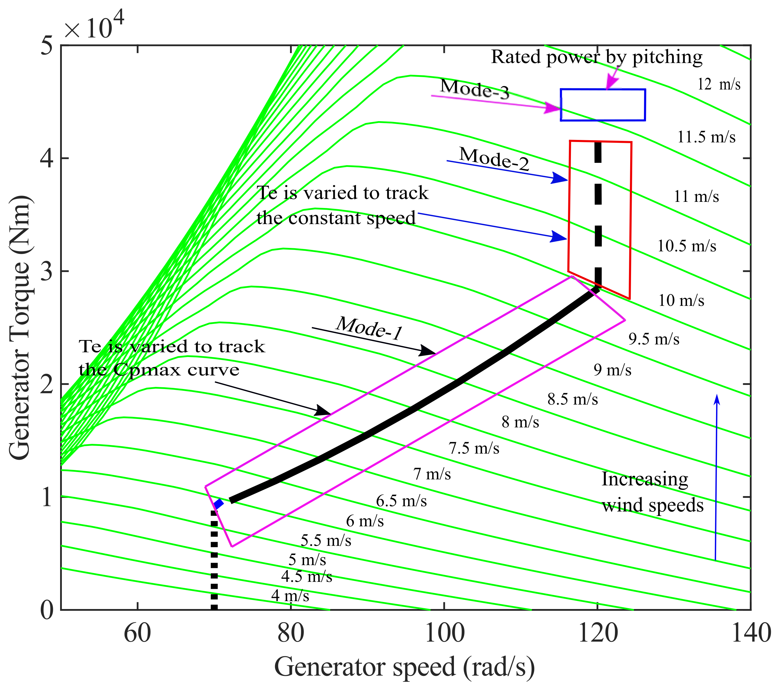
Wind turbine control consists of two parts, namely synthesis and strategy [2,3]. This paper focuses on synthesis only, which involves designing single input, single output (SISO) linear controllers using PI, or PID controllers in each operating mode. More precisely, linear controllers are frequently designed in three operating modes in the intermediate wind speeds, i.e., below-rated wind speeds (mode 1), in higher—but still just below rated—wind speeds (mode 2), and in the above-rated wind speeds (mode 3) (refer to Figure 2). Control strategy, which is not covered in this paper, includes smoothly combining these linear controllers, yielding a full envelop controller that covers the entire wind speed range (Figure 2). In order to determine the strategy, the implementation issues such as accommodation of the variation in plant dynamics over the operational envelope and switching transients and actuator constraints, which are most relevant to the application, need to be identified and the controller realisation, which best resolves them, selected. It is related to nonlinear aspects of the plant dynamics, and an investigation of the global behaviour of the system is required.
Moreover, the controllers have peculiar structures and gains in each mode, i.e., the controller exploits generator torque in modes 1 and 2 to maximize the power output and maintain a constant generator speed (), respectively. The controller also exploits the pitch angle demand in mode 3 to maintain the rated power, i.e., 5 MW in this study. In this study, a linear optimal controller is designed at mean wind speeds of 8, 10, and 16 m/s in modes 1, 2, and 3, respectively. In each mode, a linear controller is designed using pertinent control algorithms. Although most existing wind turbines are equipped with controllers that stem from the PID control, over the past decade, optimal controllers have been gaining enough attention in the literature due to their flexibility and ability to incorporate wind speed estimation/prediction into the objective functions that are only present in optimal controllers.
Optimal controller are becoming even more relevant because more wind turbines are being equipped with a LiDAR (light detection and ranging) system, which measures the upcoming wind before it impacts the turbine. In this paper, wind turbine controllers are designed using three of the most popular optimal controllers, i.e., model predictive control (MPC), linear quadratic Gaussian (LQG), and control. Thus, there is some work in the literature that reports on the design of wind turbine controllers based on optimal controllers. For example, the design of an SISO LQG controller to alleviate the fatigue loads on the blades, drive-train, and tower is reported in [4,5,6]. The design of a multi-input multi-output (MIMO) LQG controller that attempts to strike a good balance between the maximization of power output and minimization of fatigue loading is introduced in [5,6,7]. Similar work but based on MPC [8,9,10] and controller [11,12] instead of LQG [4,5,6] is available in the literature. However, to the best of the authors’ knowledge, there is no paper that provides a comparison between these optimal controllers. In this paper, MPC, LQG, and controllers are compared not only with each other but also with the standard PID controller most frequently used in industry.
In this study, optimal controllers require linear models, and the DNV Bladed models of the Supergen Wind Energy Consortium (Supergen) 5 MW exemplar turbine, which has been used for various EU and UK projects over the past 12 years, are linearised in each mode. Each linear model is attained in the state space form. Since the resulting linearized models are extremely complex, realization and tuning of optimal controllers are more difficult. Thus, these linearized models must be reduced.
Therefore, a Match-DC-gain model reduction algorithm [13] is employed. This algorithm eliminates the weakly coupled states, i.e., the states with the smallest Hankel singular values. In addition, MPC, LQG, and controllers are developed based on these linear models, and their performances are compared not only with each other but also with the standard proportional-integral-derivative (PID) controller [14].
Therefore, the main contribution of this paper is not to introduce a new control algorithm but to apply existing optimal control algorithms, i.e., MPC, LQG, and and to compare their performances. The optimal controllers are compared not only with each other but also with the controller mostly used in industry, i.e., PID. Moreover, the most significant findings of this work include that while the standard PID controller requires a drive-train damper to remove oscillation due to the drive-train mode, the optimal controllers, particularly MPC and , do not require one, thereby significantly simplifying the controller design process.
The remainder of this paper is organized as follows. The linear models, which are obtained using Bladed software, and wind speed model required to run the models are reported in Section 2. In Section 3, a brief description of control objectives and optimal controllers (MPC, , and LQG) are presented. In Section 4, the simulation results are demonstrated, followed by conclusions in Section 5.
2. Wind Turbine and Wind Speed Modelling
Linear models in this study are obtained by using the Bladed model of the Supergen Wind Energy Consortium (Supergen) 5 MW exemplar turbine. The model mainly comprises of modules of aerodynamics, rotor, drive-train, and generator. In this Section, the linear models are presented, and readers are referred to [15] for complete nonlinear models. The wind speed model required to simulate the linear models in each operating mode is also presented in this section.
2.1. Wind Speed Modelling
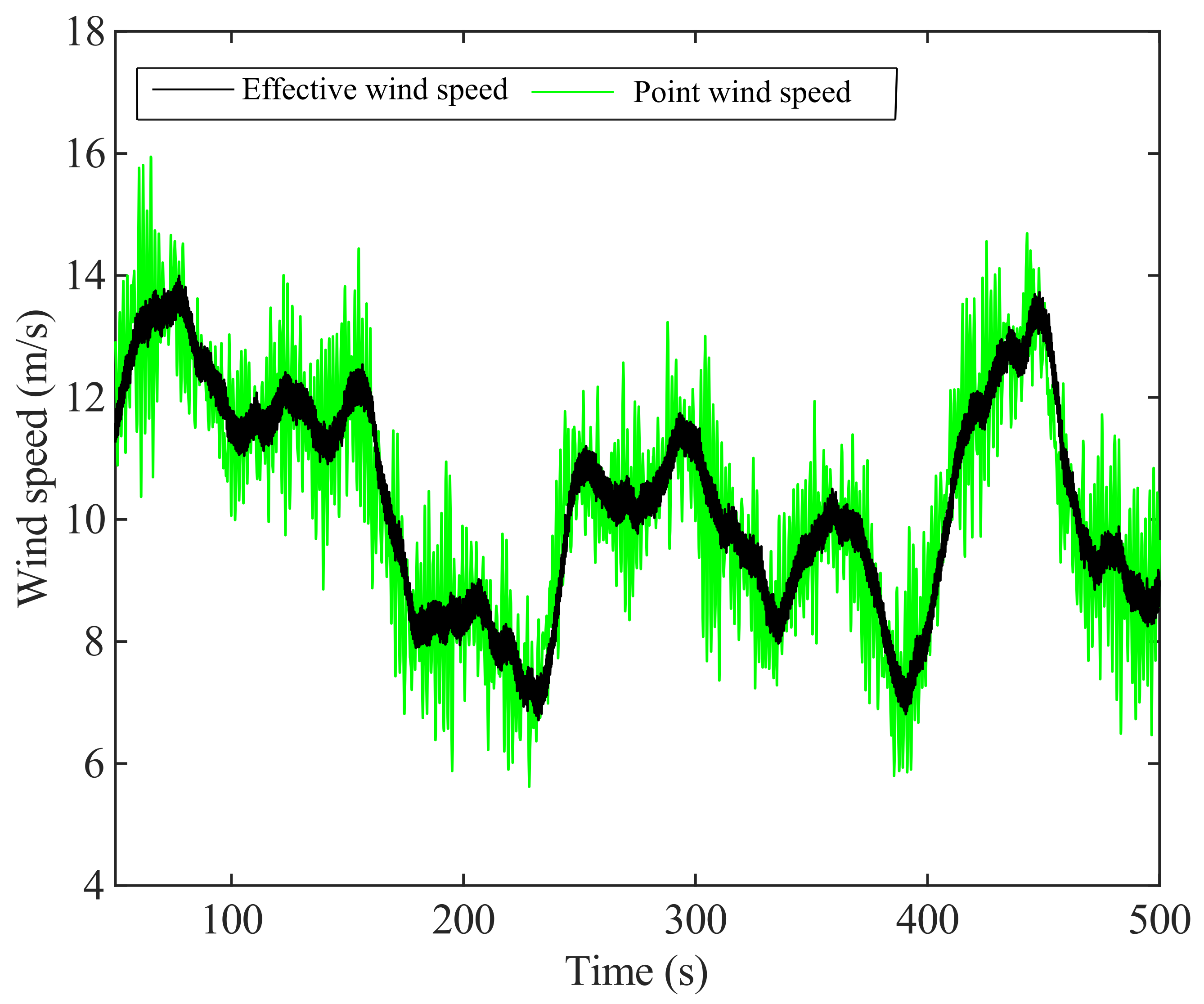
The wind arbitrarily fluctuates in space and blows toward the wind turbine. Effective wind speed is obtained by filtering the point wind speed (as measured using an anemometer) and by using the wind speed model introduced in [16]. Figure 3 shows the effective and point wind speeds used in this study. Notably, point and effective wind speeds are presented only at a mean wind speed of 10 m/s.
2.2. Linear Model of Wind Turbine Using DNV-Bladed
The linear model is obtained in state-space form by using the Bladed model of the Supergen 5 MW exemplar turbine in each operating mode as follows:
where A, B, C, and D represent the state space matrices. , , and (where n and m are three and two, respectively, at each mean wind speed, and p is 240) are defined as the following:
where , , and denote the output, input, and state, respectively. , , and are the operating points around which the models are linearized.
The inputs for the linear models are as follows:
- 1
- Generator torque;
- 2
- Pitch angle;
- 3
- Wind speed.
The outputs are as follows:
- 1
- Generator speed;
- 2
- Tower fore-aft acceleration.
As aforementioned, for the linearized models containing 240 states, making the realization and tuning of MPC, , and LQG controllers could be challenging. Consequently, in order to design optimal controllers, the models must be initially reduced. Therefore, Match-DC-Gain model reduction algorithm, which eliminates the states with the smallest Hankel singular values, is employed. The Match-DC-Gain method subsequently modifies the remaining states to retain the DC gain. For the following continuous model the procedure for the Match-DC-Gain method is as follows:
where the state vector is partitioned as follows:
where must be retained, and is discarded.
Thus, the solution is obtained by setting the derivative of to zero. The resulting reduced-order dynamic model is as follows.
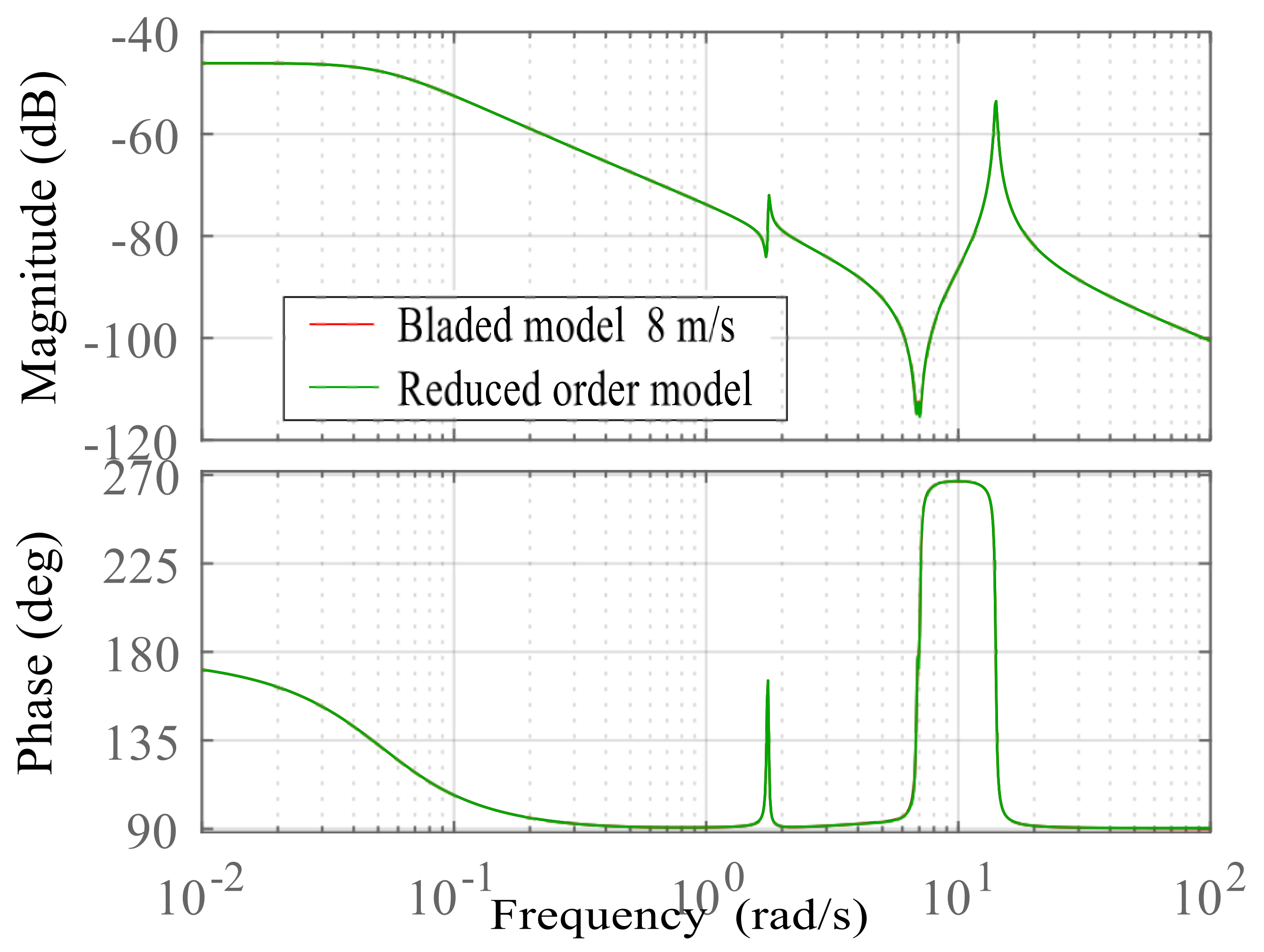
Figure 4, Figure 5 and Figure 6 show the frequency responses of the original linear models, containing 240 states in modes 1, 2, and 3, respectively, in comparison with the frequency response of the resulting reduced-order models, which now contain only 20 states due to model reduction. The results demonstrate that the original and reduced-order models exhibit identical characteristics within the meaningful frequency range, i.e., to rad/s. However, the responses diverge significantly outside of this range.
When a controller is designed in modes 1 and 2, the generator torque becomes the only input while wind speed is considered process disturbance, , and the pitch angle demand is set to zero altering Equation (1) because pitch control is not used in below-rated wind speed as follows:
where the generator torque demand is now the only input, .
Similarly, when designing a controller at above-rated wind speed, wind speed is also considered process disturbance, , and the generator torque is now set to zero because torque control is not used in above-rated wind speeds, modifying Equation (1) as follows:
where the pitch angle demand is now the only input, .
Hence, MPC, , and LQG controllers exploit the following SISO control models:
where represents generator speed, and is zero because it is assumed, in this paper, that MPC does not accept direct feedthrough. Note that although two outputs, i.e., generator speed and tower fore-aft acceleration, are available as discussed in Section 2.2 above, the controller designed here only exploits generator speed. Tower fore-aft acceleration can be used to design a tower damper [17], but this topic is not discussed in this paper.
3. Control Objectives and Optimal Control
The outline of a variable speed wind turbine control can be classified into two parts: the determination of operating strategy and its synthesis [2,3]. This study is mainly concerned with the latter. Linear controllers designed based on MPC, , and LQG are studied, and their performances are compared to achieve the control objectives. The control objectives in each operating mode are briefly explained in this Section.
For a dynamical system, optimal control is concerned with the challenge of deducing a control law that minimizes a certain objective function. A control problem comprises an objective function, which is a function of the state, and control variables. This Section summarizes the details of controllers, i.e., MPC, , and LQG. Note that MPC can be formulated equivalent to LQG if the dual-mode (or terminal cost) is used as reported in [18]. Similarly, the controller can also be embedded into the MPC formulation easily if constraints are not active as reported in [19].
3.1. Control Objectives
In below-rated wind speeds (mode 1), the generator torque, , tracks the , in order to maximize power efficiency because the curve is proportional to the generator speed, , (Figure 2). The curve in the torque/speed plane in Figure 7 (mode 1) can be represented as a parabolic function:
where k here is 1.94. Therefore, as depicted in Figure 8, the corresponding output, y, which is also the input to the controller, is defined such that the controller allows the turbine to track the curve by minimizing given by the following [3].
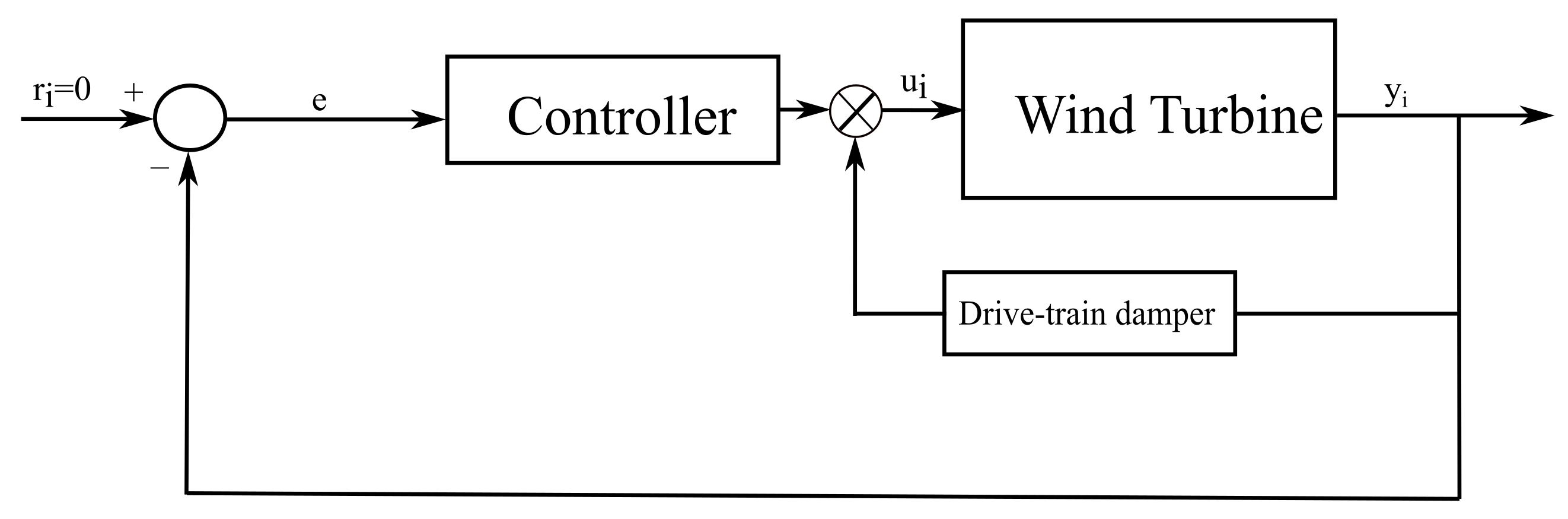
As depicted in Figure 8, a drive-train damper complements the baseline PID controller. It is a band-pass filter [17] designed to remove the oscillation caused by the drive-train mode.
In the just below-rated wind speeds, i.e., mode 2, the generator torque, , tracks the vertical line at 120 rad/s (Figure 2) by minimizing as follows.
However, the permissible generator speed fluctuations are below 12%.
In above-rated wind speeds, i.e., mode 3, the rated power, 5 MW, is maintained by active pitching. The controller tracks the rated power, 5 MW, by minimizing as follows.
Figure 7 shows that the rated power is maintained by active pitching, maintaining the generator speed fluctuations below 12%.
3.2. Model Predictive Control
MPC is a multivariable control algorithm comprising an internal dynamic model of a plant, an objective function, and an optimization algorithm minimizing the cost function, which is a function of control input u. MPC can be designed based on the linear model shown in Equation (13), which can be derived by discretizing the continuous dynamic model in Equation (8).
The MPC prediction equation can be deduced as in [18] (note that D state space matrix is zero because it is assumed, in this paper, that MPC does not accept direct feedthrough):
where p represents the prediction horizon, and can be rewritten as the following:
where c represents control horizon.
The control formulation is achieved by minimizing the following performance criteria [5]:
where it is subject to the following constraints:
where r represents the reference signal, the lower limit on , and the upper limit. is the rate of change of input, and L is a vector of ones for which their size is dependent on prediction horizon. R denotes a weighting matrix, which in this paper is tuned by trial and error. d is the residual between the measurement of y and that estimated by the internal model. This internal model could be improved by being replaced with an observer, but the usage of an observer is not considered in this paper because the internal model proves to be accurate enough.
At this stage, no constraint violation experienced. However, the full envelope controller that will be designed in the future could experience constraint violation. Therefore, an appropriate anti-wind up technique [17] will need to incorporated into the full-envelope controller in the future.
The first term in the objective function is associated with a reference tracking error, and d is incorporated to provide offset corrections and unbiased predictions. The second term in the optimization function lowers the control effort. Hence, R allows a trade-off between these two contradictory problems. denotes measured states at each time step, which originate from the plant’s internal model.
The procedure for MPC controller implementation can be summarized as follows:
- 1
- The current plant states are measured at each time step, and the control sequence is determined by solving the objective function over a future prediction horizon.
- 2
- Only the first value is applied to the system; the remaining values are removed. Furthermore, the plant states are sampled, and the objective function is recalculated starting from the new current states.
- 3
- MPC is also called receding horizon control since the prediction horizon keeps moving forward.
3.3. Control
control is revised in this section. It is a multivariable control algorithm consisting of generalized plant, P(s) as shown in Equation (18), and minimization of optimization function according to norm. control is formulated based on the system considered by the following:
with a state-space form of the generalized plant P(jw) given by the following.
The plant has two input signals: the manipulated variables, u, and denotes exogenous signal that comprises disturbance, reference signals, etc. In addition, there are two output signals, the error signals , which include reference tracking error and control effort which are to be minimized, and the measured variable y. Therefore, the closed-loop transfer function from w to z is given by the following linear fractional transformation:
where the following is the case.
Hence, the main goal of the control problem is to design a controller, K, that minimizes the according to the norm. The infinity norm of matrix transfer function is defined as follows:
where is the maximum singular value of the matrix .
3.4. Linear Quadratic Gaussian Control
A linear quadratic Gaussian is a combination of a linear quadratic regulator (LQR) and Kalman filter [20,21]. LQR regulates the plant using the states, which can be estimated from the Kalman filter. Notably, the system (plant) is affected by process and measurement noises. LQG control provides the optimal control input to the system (plant) by diminishing the effect of process and measurement noises. LQG is summarized as follows.
LQR solves the optimization problem offline:
where R is an symmetric positive semi-definite matrix, and is an symmetric positive semi-definite matrix. Both matrices are tuned by trial and error. The first and second parts in the optimization function are the minimization of error between the reference and measured value and the minimization of the control effort, respectively.
The solution to this LQR controller can be written in terms of the simple state feedback law by minimizing the performance index, J, in Equation (24) as a simple matrix gain of the following form:
where is the state estimates from the Kalman filter, and K is a matrix as follows:
where X is the unique positive-definite matrix obtained from solving the continuous algebraic Riccati equation as follows.
Kalman Filter
Plant dynamics are corrupted by disturbance signals (process noise) and measurement noise. Thus, we have a plant model of the following:
where and are the disturbance (process noise) and measurement noise inputs, respectively, i.e., and are white noise processes with covariances. The inferences can be summarized as follows.
The Kalman filter has the layout of a standard state estimator or observer, as follows.
The estimator or observer uses the output, y(t), and inputs, u(t) to produce the estimated output, , and estimated state, .
The optimal solution of is obtained by minimizing the J as follows:
where P = is a steady-state error covariance matrix obtained by solving the continuous algebraic Riccati equation as follows.
4. Simulation Results
In this section, all optimal controllers are compared with one another and with a standard PID controller in the frequency and time domains, as well as on the torque/speed plane.
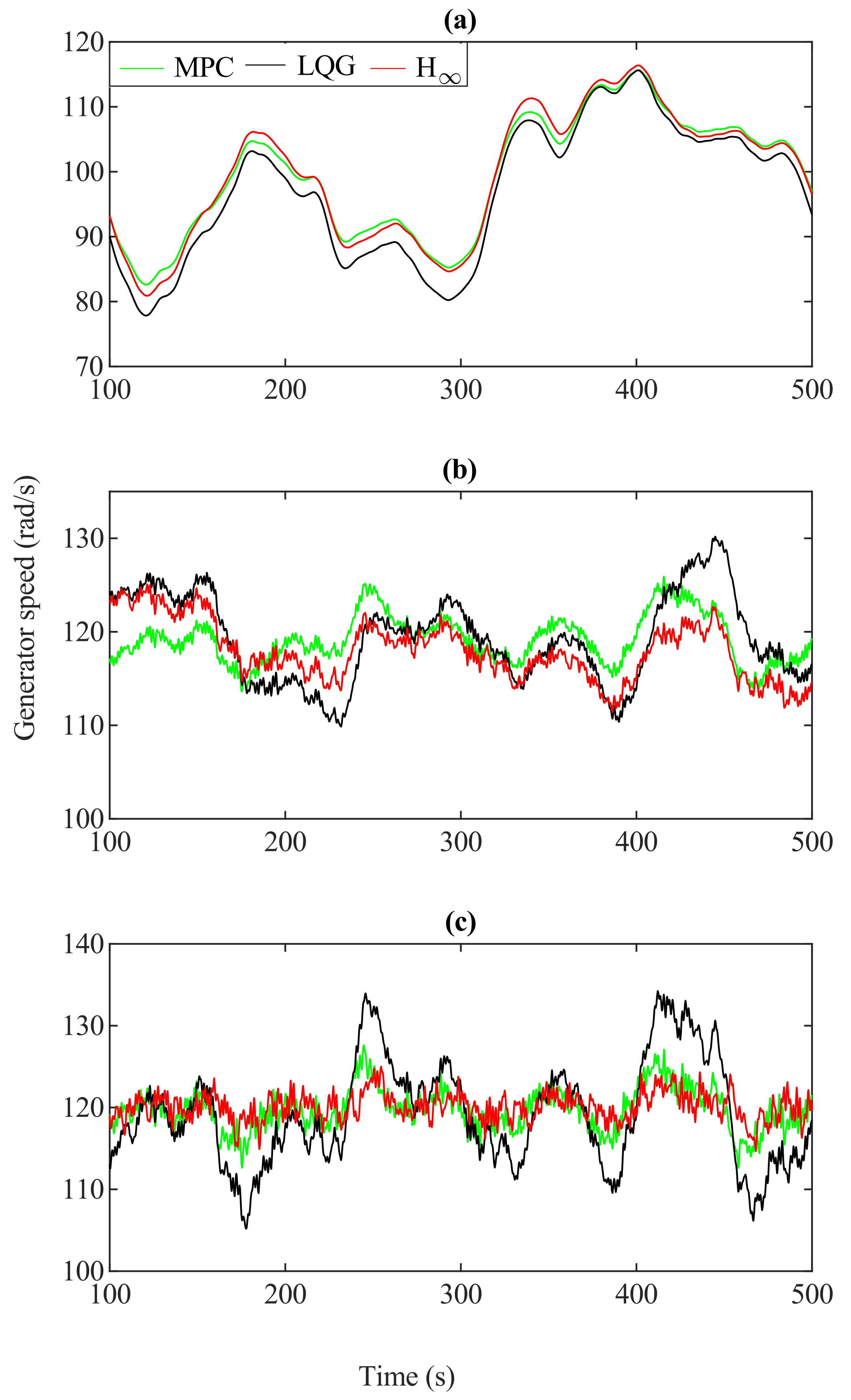
Figure 9 depicts the measured output at each mean wind speed (i.e., generator speed). Figure 9a shows the time responses for the MPC, LQG, and controllers in mode 1. It is difficult to confirm if the curve is tracked, which is the control objective in the time domain as discussed in Section 3.1, i.e., in Figure 9a. However, tracking of the curve is better presented on the torque/speed plane in Figure 10. The figure demonstrates how all the optimal controllers, MPC (in red), (in blue), and LQG (in black), perform on the torque/speed plane. They all appear to be satisfactory in closely tracking the curve. The corresponding time responses of the power output for the MPC, LQG, and controllers at a mean wind speed of 8 m/s (below-rated wind speed, i.e., mode 1) are illustrated in Figure 11a.
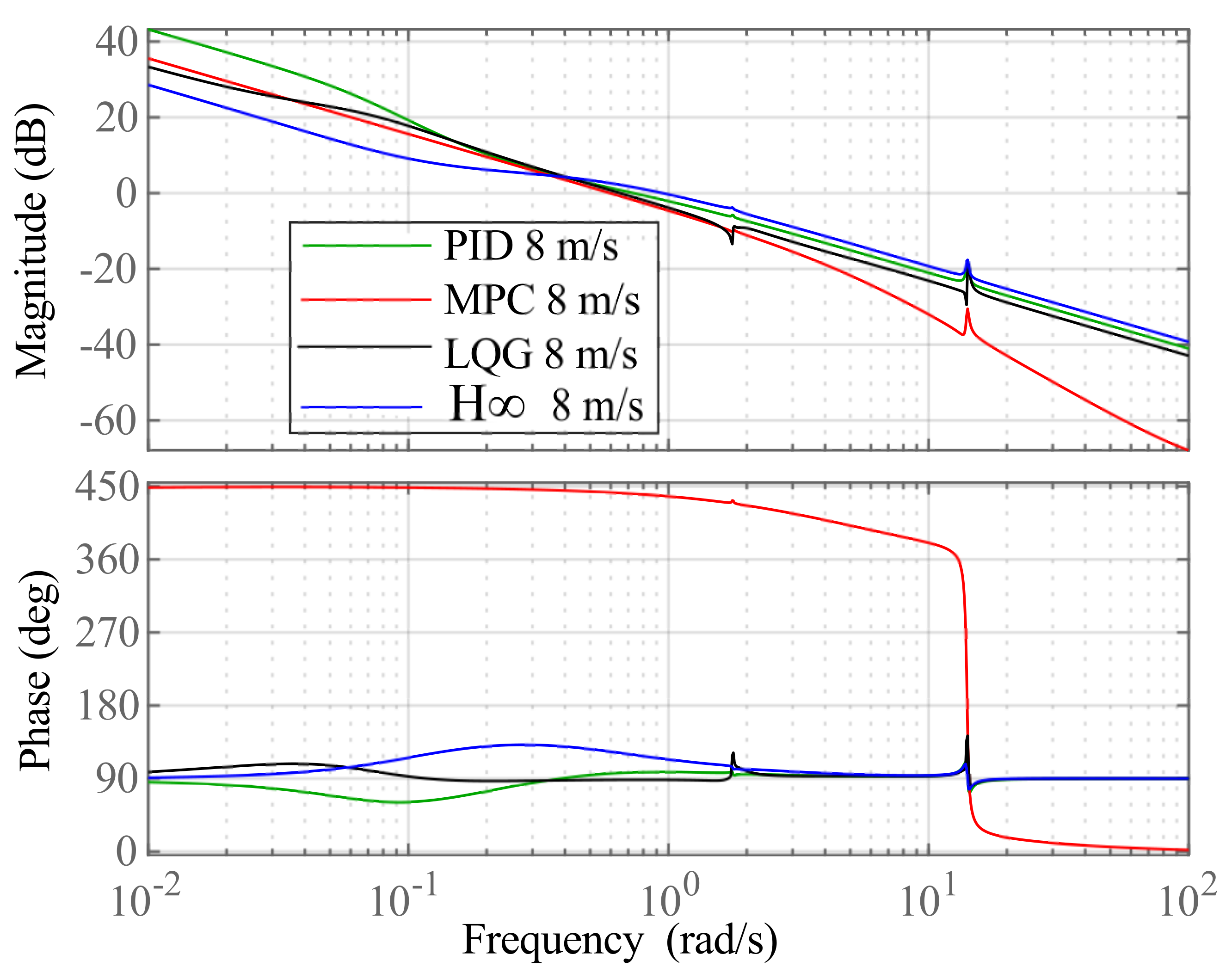
Controller performance is also interpreted in the frequency domain, i.e., open-loop frequency response (Figure 12). The open-loop system [22] () in Figure 8 is considered the product of the controller (open-loop) and the process (i.e., wind turbine ). The controllers should achieve a gain crossover frequency in the range of 0.6 to 2 rad/s due to wind characteristics [23]. Gain crossover frequencies below 0.6 rad/s could cause an extremely slow control action, whereas those above 2 rad/s could cause an aggressive control action, potentially resulting in saturation of actuator, particularly in high wind speeds, i.e., in the above-rated region.
In mode 1, Figure 12 shows that the gain crossover frequencies of the controllers (MPC, LQG, and ) are approximately between 0.6 and 2 rad/s. Notably, that PID controller is included in this study for comparison purposes only. The implication is that these controllers are neither too aggressive nor too slow.
In summary, the time response in Figure 9a, results on torque/speed plane in Figure 10, and open-loop frequency responses in Figure 12 all show that the overall performance of these optimal controllers are satisfactory.
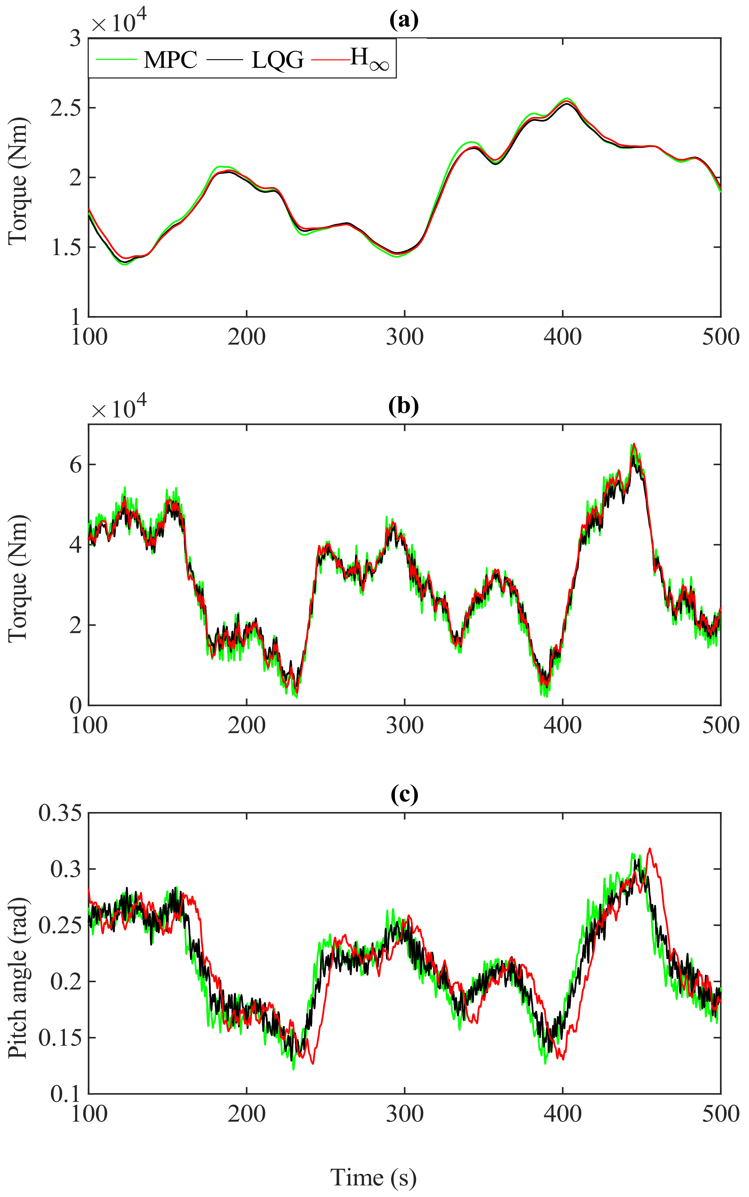
Figure 13a shows the corresponding control input, i.e., torque demand in mode 1. Control of generator speed is achieved by adjusting torque in mode 1, as aforementioned.
As depicted in Figure 9b the time responses of the MPC, LQG, and controllers in mode 2 are adequate in terms of fluctuations, as they persist under 12%. Table 1 summarizes the results of generator speed fluctuations of all optimal controllers in mode 2; it shows the mean fluctuations for each controller in mode 2. The results show that fluctuations appear satisfactory because they remain below 12%. The corresponding time responses of the power output of the MPC, LQG, and controllers at a mean wind speed of 10 m/s (just below-rated wind speeds, i.e., mode 2) are illustrated in Figure 11b.
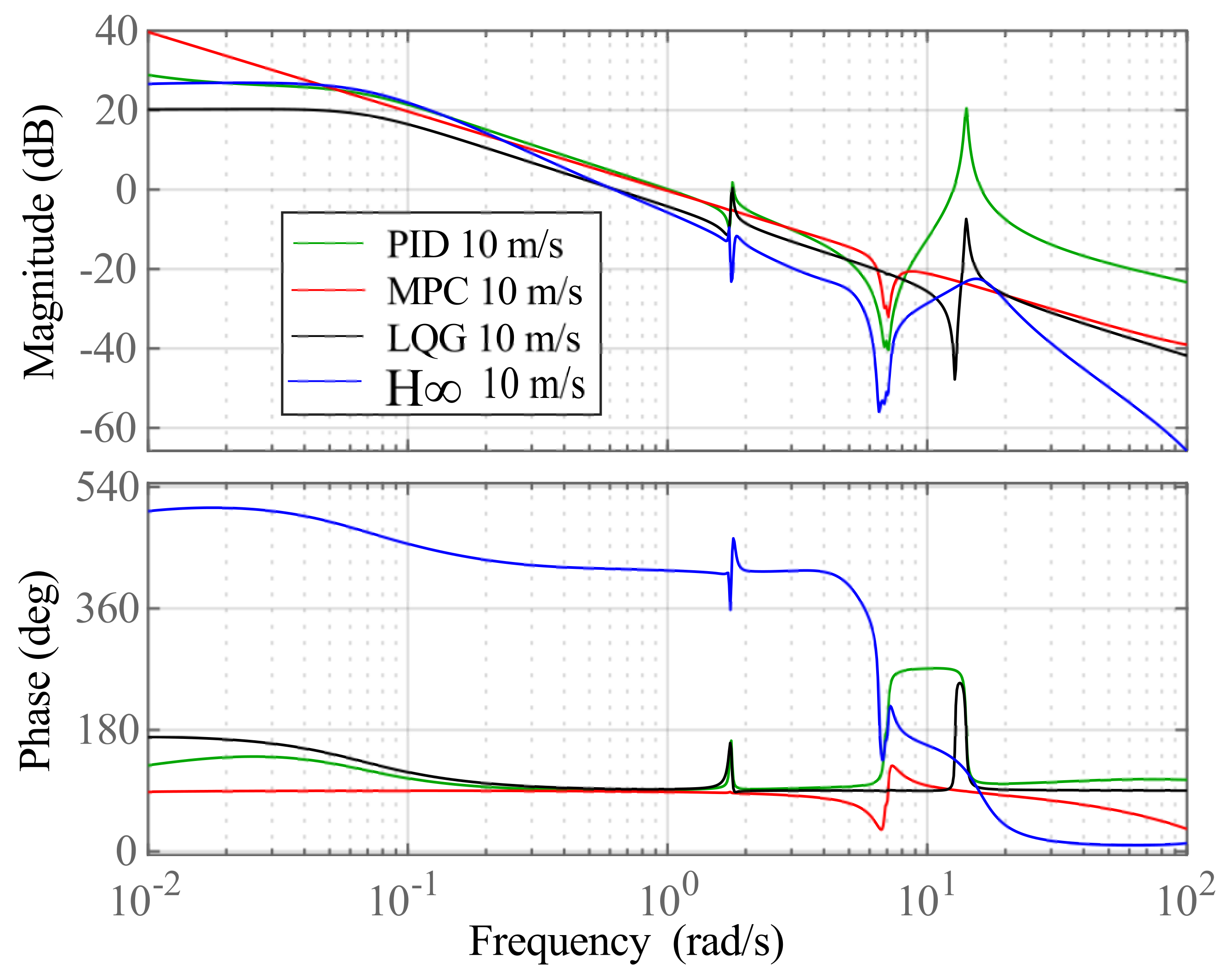
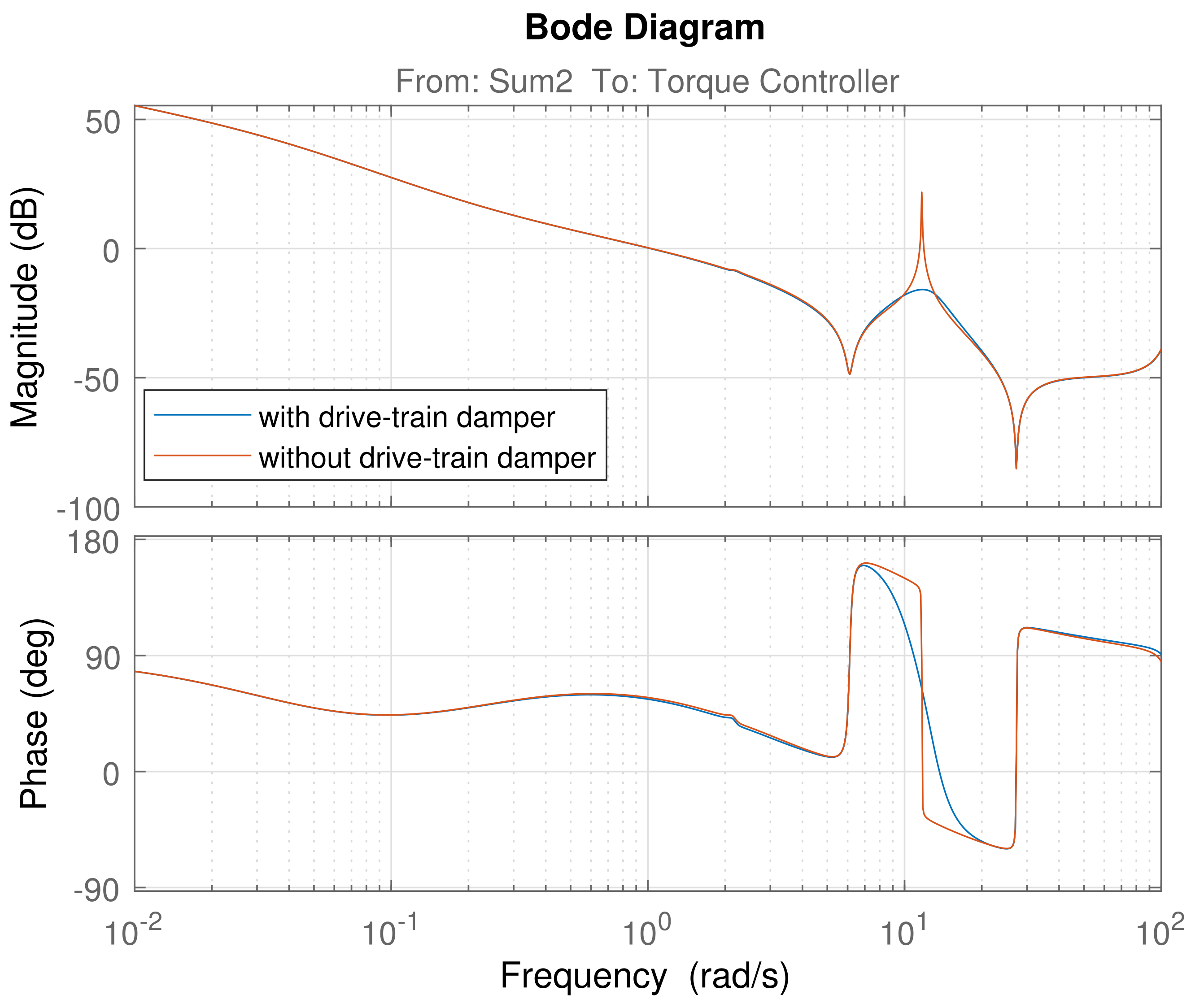
The controller performance is also interpreted in the frequency domain. Figure 14 shows that at a mean wind speed of 10 m/s and the gain crossover frequencies of the controllers (MPC, LQG, and ) are in the range of 0.6 to 2 rad/s, which is satisfactory as aforementioned. Note that, again, the PID controller is also included here for comparison purposes only. The results imply that these controllers are neither extremely aggressive nor slow. However, for the PID controller, the peaks at about 14.13 rad/s persist mostly above 0 dB, which corresponds to the drive-train mode, indicating that the controller would be sensitive to noise and uncertainty; hence, it is not robust. Furthermore, these peaks are eliminated by employing a drive-train damper [17]; i.e., the PID controller requires a drive-train damper to maintain the peak at about 14.13 rad/s below 0 dB (Figure 15). Furthermore, the red and blue plots represent the open-loop frequency responses without and with drive-train damper, respectively. Figure 15 shows the open-loop frequency response of the PID controller when a drive-train damper (in blue) is used, compared with the open-loop frequency response of the PID controller when a drive-train damper (in red) is not used.
Figure 15 shows that the damper removes the peak at 14.13 rad/s, which is due to the drive-train mode. Thus, oscillation due to the drive-train mode is removed. However, the drive-train damper is not required when the optimal controllers are in place (Figure 14), which is a significant advantage over standard PID controllers.
In summary, the time responses shown in Figure 9b, results presented in Table 1, and open-loop frequency responses shown in Figure 14 show that the overall performance of these optimal controllers are satisfactory. In contrast to the PID controller, the MPC and controllers exhibit better performance than the LQG controller because the peak still remains when the LQG controller is in place although it is maintained below 0 dB.
Figure 13b shows the corresponding control input, i.e., torque demand in mode 2. Generator speed control is achieved by adjusting torque in mode 2 as aforementioned.
Figure 9c shows that the time responses for the MPC, LQG, and controllers at a mean wind speed of 16 m/s are adequate in terms of fluctuations as they persist under 12%. Table 1 summarizes the results for generator speed fluctuations of all optimal controllers in mode 3. It depicts that fluctuations are adequate as they persist below 12% which is within the controller design specifications mentioned in Section 3.1. Figure 11c illustrates the corresponding time response of the power output of the MPC, LQG, and controllers at a mean wind speed of 16 m/s (above-rated wind speeds, i.e., mode 3).
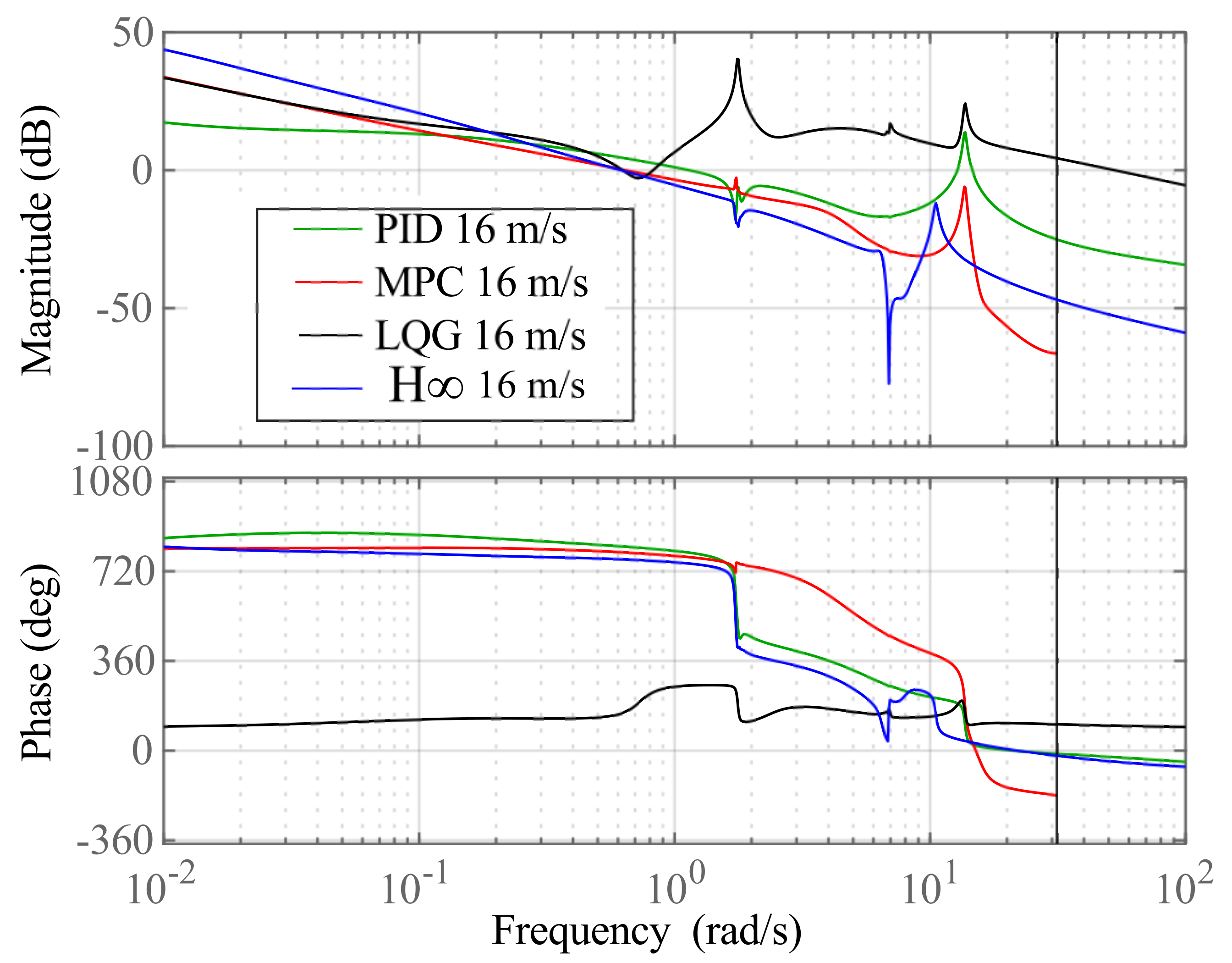
Furthermore, modes 1 and 2 controller performances are also interpreted in the frequency domain. Figure 16 shows that, the gain crossover frequencies of the controllers (MPC, LQG, and ) at a mean wind speed of 16 m/s are in the range of 0.6 to 2 rad/s. Note that the PID controller is included here for comparison only. The results imply that these controllers are neither extremely aggressive nor slow. However, the peak corresponding to the drive-train mode for the PID and LQG controllers remain mostly above 0 dB at about 13.75 rad/s (higher frequency range), indicating that the controller’s sensitivity to noise and uncertainty is high. These peaks are removed by incorporating a drive-train damper [17]; i.e., the PID controllers require a drive-train damper to maintain the peak at around 13.75 rad/s below 0 dB (Figure 15). However, MPC and controllers achieve the same results without incorporating such dampers, i.e., in contrast to modes 1 and 2, the peak remains present but is below 0 dB. Nonetheless, these controllers in mode 3 are more sensitive than those in mode 2.
In summary, the time responses of the generator speed shown in Figure 9c, the output power shown in Figure 11c, results presented in Table 1, and open loop frequency responses indicate that the overall performance of the optimal controllers, particularly MPC and controllers, outperform PID controllers, as illustrated in the frequency domain.
Figure 13c shows the corresponding control input, i.e., pitch angle demand in mode 3. Generator speed control is achieved by adjusting the pitch angle in mode 3, as aforementioned.
The results discussed so far are summarized in Table 2. It introduces the performance of all optimal controllers using error metrics. As aforementioned, the curve is tracked in order to extract as much energy as possible from the wind in mode 1; in mode 2, the constant generator speed () is tracked; and the rated power is maintained in mode 3 by active pitching. Table 2 illustrates that, in mode 1, all optimal controllers appear to be satisfactory in terms of tacking the curve. In mode 2, all optimal controllers appear to satisfactorily track the constant generator speed (). In mode 3, all optimal controllers appear to satisfactorily maintain the rated power.
5. Conclusions
In this study, a linear model is obtained by using the Bladed model of the Supergen Wind Energy Consortium (Supergen) 5 MW exemplar turbine model in different modes. These linear models are complex; hence, the realization and tuning of optimal controllers can be more challenging. Thus, the models must be reduced in order to design optimal controllers. Therefore, the Match-DC-Gain model reduction algorithm is used to reduce the model. The resulting models are similar to the original models in the meaningful frequency range. Based on these linear models MPC, , and LQG controllers are synthesized in each mode and compared with each other and with the standard PID controller, which is also included for comparison.
Simulation results demonstrate that in, mode 1, all optimal controllers show satisfactory performances not only in time and frequency domain but also in the torque/speed plane. In mode 2, the open-loop frequency responses demonstrate that the optimal controllers, especially the MPC and controllers, outperform the standard PID controllers. In more detail, the PID controller requires a drive-train damper to remove oscillation due to the drive-train mode, and designing such a damper could be challenging. However, when the optimal controllers are used, the oscillation due to the drive-train mode is removed without having to incorporate a drive-train damper. In mode 3, only the MPC and controllers can be designed without having to incorporate a drive-train damper. The LQG controller needs to incorporate a drive-train damper similar to the PID controller, making the LQG controller less competitive than the other optimal controllers. Furthermore, the MPC and controllers are more sensitive than those in mode 2; hence, extra care should be taken when designing MPC and controllers in mode 3. In summary, the MPC and controller perform most satisfactorily because they can achieve performance on a par with the PID controller, without incorporating a drivetrain damper that is compulsory in the PID design. The LQG controller performs as well as the other optimal controllers only in mode 2, but it is more sensitive and harder to tune than the other controllers overall.
As discussed in Section 1, wind turbine control involves both the determination of the operating strategy of the controller and its synthesis. This paper only discusses synthesis, which is concerned with designing SISO linear controllers at different operating points or modes. Further research will involve the operating strategy, which will allow the linear controllers designed in this paper to be combined by introducing an appropriate switching method to obtain the full envelope controller that covers the full operational envelope of wind speed. Finally, in this paper, the optimal controllers are designed as SISO controllers, but designing the optimal controllers as an MIMO controllers, which could be more efficient, will also be considered.
Author Contributions
Conceptualization, S.-h.H. and Y.-s.R.; methodology, S.-h.H.; software, Y.-s.R.; validation, S.-h.H. and Y.-s.R.; formal analysis, S.-h.H.; investigation, Y.-s.R. and S.-h.H.; resources, S.-h.H. and Y.-s.R.; data curation, Y.-s.R.; writing—original draft preparation, Y.-s.R. and S.-h.H.; writing—review and editing, Y.-s.R.; visualization, S.-h.H. and Y.-s.R.; supervision, S.-h.H.; project administration, S.-h.H.; funding acquisition, S.-h.H. All authors have read and agreed to the published version of the manuscript.
Funding
This work was supported in part by the Korea Institute of Energy Technology Evaluation and Planning (KETEP) grant funded by the Korean government (MOTIE) (20203020020020, Feasibility Study on 40 years Life Wind Turbine) and the Korea Electric Power Corporation (R21XO01-17).
Institutional Review Board Statement.
Not applicable.
Informed Consent Statement.
Not applicable.
Data Availability Statement.
Not applicable.
Conflicts of Interest
The authors declare no conflict of interest.
References
- Council, G.W.E. Gwec/Global Wind Report 2021; Global Wind Energy Council: Brussels, Belgium, 2021. [Google Scholar]
- Garcia-Sanz, M.; Houpis, C.H. Wind Energy Systems: Control Engineering Design; CRC Press: Boca Raton, FL, USA, 2012. [Google Scholar]
- Leithead, W.; Connor, B. Control of variable speed wind turbines: Design task. Int. J. Control 2000, 73, 1189–1212. [Google Scholar] [CrossRef]
- Nourdine, S.; Camblong, H.; Vechiu, I.; Tapia, G. Comparison of wind turbine LQG controllers using individual pitch control to alleviate fatigue loads. In Proceedings of the 18th Mediterranean Conference on Control and Automation, MED’10, Marrakech, Morocco, 23–25 June 2010; pp. 1591–1596. [Google Scholar]
- Grimble, M.J.; Johnson, M.A. Optimal Control and Stochastic Estimation: Theory and Applications; John Wiley & Sons: Hoboken, NJ, USA, 1988; Volume 1. [Google Scholar]
- Trentelman, H.L.; Stoorvogel, A.A.; Hautus, M. Control Theory for Linear Systems; Springer Science & Business Media: Berlin/Heidelberg, Germany, 2012. [Google Scholar]
- Pintea, A.; Wang, H.; Christov, N.; Borne, P.; Popescu, D.; Badea, A. Optimal control of variable speed wind turbines. In Proceedings of the 2011 19th Mediterranean Conference on Control & Automation (MED), Corfu, Greece, 20–23 June 2011; pp. 838–843. [Google Scholar]
- Kong, X.; Ma, L.; Liu, X.; Abdelbaky, M.A.; Wu, Q. Wind turbine control using nonlinear economic model predictive control over all operating regions. Energies 2020, 13, 184. [Google Scholar] [CrossRef] [Green Version]
- Camacho, E.; Bodons, C. Model Predictive Control in the Process Industry: Advances in Industrial Control; Springer: London, UK, 1995. [Google Scholar]
- Grancharova, A.; Johansen, T.A. Explicit Nonlinear Model Predictive Control: Theory and Applications; Springer Science & Business Media: Berlin/Heidelberg, Germany, 2012; Volume 429. [Google Scholar]
- Pintea, A.; Christov, N.; Borne, P.; Popescu, D. H∞ controller design for variable speed wind turbines. In Proceedings of the 18-th International Conference on Control Systems and Computer Science, Bucharest, Romania, 24–27 May 2011. [Google Scholar]
- Skogestad, S.; Postlethwaite, I. Multivariable Feedback Control: Analysis and Design; John Wiley and Sons: Chichester, UK, 2007; Volume 2. [Google Scholar]
- Varga, A. Balancing free square-root algorithm for computing singular perturbation approximations. In Proceedings of the 30th IEEE Conference on Decision and Control, Brighton, UK, 11–13 December 1991; pp. 1062–1065. [Google Scholar]
- Ang, K.H.; Chong, G.; Li, Y. PID control system analysis, design, and technology. IEEE Trans. Control. Syst. Technol. 2005, 13, 559–576. [Google Scholar]
- Hur, S.; Recalde-Camacho, L.; Leithead, W. Detection and compensation of anomalous conditions in a wind turbine. Energy 2017, 124, 74–86. [Google Scholar] [CrossRef] [Green Version]
- Leithead, W. Effective wind speed models for simple wind turbine simulations. In Proceedings of the British Wind Energy Conference, Nottingham, UK, 25–27 March 1992; Mechanical Engineering Publications: London, UK, 1992; pp. 321–326. [Google Scholar]
- Chatzopoulos, A.P. Full Envelope Wind Turbine Controller Design for Power Regulation and Tower Load Reduction. Ph.D. Thesis, University of Strathclyde, Glasgow, UK, 2011. [Google Scholar]
- Rossiter, J.A. Model-Based Predictive Control: A Practical Approach; CRC Press: Boca Raton, FL, USA, 2003. [Google Scholar]
- Lio, W.; Jones, B.L.; Rossiter, J. Preview predictive control layer design based upon known wind turbine blade-pitch controllers. Wind Energy 2017, 20, 1207–1226. [Google Scholar] [CrossRef] [Green Version]
- Maciejowski, J.M. Predictive Control: With Constraints; Pearson Education: London, UK, 2002. [Google Scholar]
- Clements, D.; BDO, A. Singular Optimal Control: The Linear Quadratic Problem; Springer: Berlin/Heidelberg, Germany, 1978. [Google Scholar]
- Dorf, R.C.; Bishop, R.H. Modern Control Systems; Pearson Prentice Hall: Hoboken, NJ, USA, 2008. [Google Scholar]
- Leith, D.J.; Leithead, W.E. Appropriate realization of gain-scheduled controllers with application to wind turbine regulation. Int. J. Control 1996, 65, 223–248. [Google Scholar] [CrossRef]
Figure 1.
Horizontal axis variable speed wind turbine.

Figure 2.
Turbine behaviour on torque/speed plane.

Figure 3.
Point wind speed (green) vs. effective wind speed (black) at a mean wind speed of 10 m/s.

Figure 4.
Frequency response of Bladed and reduced–order models in mode 1.

Figure 5.
Frequency response of Bladed and reduced–order models in mode 2.

Figure 6.
Frequency response of Bladed and reduced–order models in mode 3.

Figure 7.
Control objective in each operating mode on torque/speed plane.

Figure 8.
Control scheme.

Figure 9.
Time responses of control output (generator speed) in modes 1, 2, and 3: MPC, LQG, and based on the Bladed linearization model; (a) mode 1, (b) mode 2, (c) mode 3.
Figure 9.
Time responses of control output (generator speed) in modes 1, 2, and 3: MPC, LQG, and based on the Bladed linearization model; (a) mode 1, (b) mode 2, (c) mode 3.

Figure 10.
Behaviour of MPC, LQG, and controllers in mode 1 on torque/speed plane.

Figure 11.
Time responses of power in modes 1, 2, and 3: MPC, LQG, and based on Bladed linearization model; (a) mode 1, (b) mode 2, (c) mode 3.
Figure 11.
Time responses of power in modes 1, 2, and 3: MPC, LQG, and based on Bladed linearization model; (a) mode 1, (b) mode 2, (c) mode 3.

Figure 12.
Open–loop frequency responses of PID, MPC, LQG, and based on Bladed linearized model in mode 1.
Figure 12.
Open–loop frequency responses of PID, MPC, LQG, and based on Bladed linearized model in mode 1.

Figure 13.
Time responses of torque and pitch angle demand (control input) in mode 1 and 2 and mode 3, respectively: MPC, LQG, and based on Bladed linearization model; (a) mode 1, (b) mode 2, (c) mode 3.
Figure 13.
Time responses of torque and pitch angle demand (control input) in mode 1 and 2 and mode 3, respectively: MPC, LQG, and based on Bladed linearization model; (a) mode 1, (b) mode 2, (c) mode 3.

Figure 14.
Open–loop frequency responses of PID, MPC, LQG, and controllers based on Bladed linearized model in mode 2.
Figure 14.
Open–loop frequency responses of PID, MPC, LQG, and controllers based on Bladed linearized model in mode 2.

Figure 15.
Open–loop frequency responses of PID controller with and without damper.

Figure 16.
Open–loop frequency responses of PID, MPC, LQG, and controllers based on Bladed linearized model in mode 3.
Figure 16.
Open–loop frequency responses of PID, MPC, LQG, and controllers based on Bladed linearized model in mode 3.


Table 1.
Mean of percentage of speed fluctuations.
| Operating Mode | MPC | LQG | |
|---|---|---|---|
| Mode 2 | 5.36 | 7.36 | 9.45 |
| Mode 3 | 4.49 | 3.91 | 9.39 |
Table 2.
Controllers performance in each mode.
| MPC | LQG | ||
|---|---|---|---|
| Mean power efficiency in Mode 1 | 99.11 | 98.50 | 98.14 |
| RMSE of | |||
| in Mode 2 | 2.55 | 3.523 | 2.023 |
| RMSE of | |||
| in Mode 3 | 1.9310 | 1.8972 | 3.0723 |
: constant generator speed, 120 rad/s; : rated power, 5 MW.
Publisher’s Note: MDPI stays neutral with regard to jurisdictional claims in published maps and institutional affiliations. |
© 2021 by the authors. Licensee MDPI, Basel, Switzerland. This article is an open access article distributed under the terms and conditions of the Creative Commons Attribution (CC BY) license (https://creativecommons.org/licenses/by/4.0/).
Share and Cite
MDPI and ACS Style
Reddy, Y.-s.; Hur, S.-h. Comparison of Optimal Control Designs for a 5 MW Wind Turbine. Appl. Sci. 2021, 11, 8774. https://0-doi-org.brum.beds.ac.uk/10.3390/app11188774
AMA Style
Reddy Y-s, Hur S-h. Comparison of Optimal Control Designs for a 5 MW Wind Turbine. Applied Sciences. 2021; 11(18):8774. https://0-doi-org.brum.beds.ac.uk/10.3390/app11188774
Chicago/Turabian StyleReddy, Yiza-srikanth, and Sung-ho Hur. 2021. "Comparison of Optimal Control Designs for a 5 MW Wind Turbine" Applied Sciences 11, no. 18: 8774. https://0-doi-org.brum.beds.ac.uk/10.3390/app11188774
Note that from the first issue of 2016, this journal uses article numbers instead of page numbers. See further details here.