
Container Volume Prediction Using Time-Series Decomposition with a Long Short-Term Memory Models


Industrial Data Science and Engineering, Department of Industrial Engineering, Pusan National University, 2 Busandaehak-ro 63beon-gil, Geumjeong-gu, Busan 46241, Korea
*
Author to whom correspondence should be addressed.
Appl. Sci. 2021, 11(19), 8995; https://0-doi-org.brum.beds.ac.uk/10.3390/app11198995
Submission received: 10 August 2021
/
Revised: 19 September 2021
/
Accepted: 24 September 2021
/
Published: 27 September 2021
(This article belongs to the Special Issue Big Data and AI for Process Innovation in the Industry 4.0 Era, Volume II)
Abstract
:The purpose of this study is to improve the prediction of container volumes in Busan ports by applying external variables and time-series data decomposition methods to deep learning prediction models. Previous studies on container volume forecasting were based on traditional statistical methodologies, such as ARIMA, SARIMA, and regression. However, these methods do not explain the complexity and variability of data caused by changes in the external environment, such as the global financial crisis and economic fluctuations. Deep learning can explore the inherent patterns of data and analyze the characteristics (time series, external environmental variables, and outliers); hence, the accuracy of deep learning-based volume prediction models is better than that of traditional models. However, this does not include the study of overall trends (upward, steady, or downward). In this study, a novel deep learning prediction model is proposed that combines prediction and trend identification of container volume. The proposed model explores external variables that are related to container volume, combining port volume time-series decomposition with external variables and deep learning-based multivariate long short-term memory (LSTM) prediction. The results indicate that the proposed model performs better than the traditional LSTM model and follows the trend simultaneously.
1. Introduction
Deep learning is a type of machine learning in which the design of algorithms like artificial neural networks is inspired by the working of the human brain; additionally, the algorithms learn from large amounts of data [1]. Deep learning algorithm generally utilizes hidden layers that are learned through various combinations in deep neural networks. Hidden layers are all layers between the input layer and the output layer which compose the deep neural networks.
This type of learning exhibits human-level performance in various fields, such as image recognition, text classification, and speech recognition. It is also useful as an analytical model for prediction in diverse disciplines, such as economy, medicine, and physics. As time-series data is widely represented in various fields, container volume data is one of the representative time series data in the port sector. Deep learning neural networks are capable of automatically learning complex mappings from inputs to outputs and support multiple inputs and outputs, thus demonstrating good performance in the long-term predictive performance of time-series data [1]. Thus, a time-series prediction model with deep learning can easily deal with multicollinearity or nonlinear problems that are not addressed by traditional statistical models [2].
In this study, we applied deep learning prediction models to container volume predictions, which are in a sense, representative time-series data, to yield better prediction results. Container volume data is representative continuous time-series data that have been actively studied by statistical models from researchers. Previous studies on container volume prediction have implemented models, such as autoregressive integrated moving average (ARIMA), seasonal autoregressive integrated moving average (SARIMA), and traditional regression. However, the limitation of traditional time-series prediction techniques is that the performance reduces when unexpected variations are reflected in the data [3]. Various external factors, such as the financial crisis and internal and external economic impacts reduce the stability of time-series data
In particular, Busan Port, known as the largest port in Korea, has gained interest from many researchers in utilizing deep learning models with time-series prediction. The container volume prediction at Busan port in Korea, indicated that the development of the port is closely related to national competitiveness and in fact, strengthens it; hence, accurate prediction of container volume is essential [4]. In an effort to strengthen the Busan port in Korea, the study of predicting container volume at Busan Port has been expanded from statistical methodology to univariate prediction, and multivariate prediction by deep learning models.
Deep learning is broadly used in container volume prediction analysis models, wherein univariate time-series data are combined with deep learning models [4]. Deep learning-based container volume prediction shows improved results over traditional statistical models. Not only a univariate prediction but also a combination of deep learning-based models with external variables improves flexibility and increases the model’s variability acceptance from the data. A multivariate time-series prediction model that includes external variables is appropriate for more delicate container volume predictions. Combinations of external variables give an important glimpse of utilizing essential factors in deep learning that could be enriched in the prediction.
Thus, in this study, we seek to explore and apply external variables that are relevant to the container volume predictions. The selection criteria are correlations and trends that have proven influence according to previous research works [5,6]. We applied various external factors from the previous studies on the container volume prediction literature, then conduct each variable with the vector auto regressive (VAR) model. After validating variables by the VAR model, we apply into ordinary deep learning models with external variables and without external variables to validate the prediction performance improvements in various aspects.
From our study, the contributions of this study are as follows: (1) We propose a time-series decomposition method to predict the container volume in detail considering the performance and the trend followability at the same time; (2) we utilized various external variables used from previous studies in order to confirm the effectiveness of each variable by VAR model; (3) we provide the advantages of a time-series decomposition method that can effectively mitigate the errors from one another and ultimately improves the performance of the prediction.
The remainder of this paper is organized as follows. Section 2 provides an overview of time-series analysis, deep learning prediction, and deep learning in container volume prediction. Section 3 describes the data analysis of the container volume and explores external variables for the implications, which is validated by a statistical model called the VAR model; this is followed by a description of the proposed method of time-series decomposition. Section 4 provides the results derived from our experiments and compares them with the results of various other time-series prediction models. Finally, Section 5 summarizes the discussion based on our experiments and Section 6 presents the conclusions along with future research ideas.
2. Background
This section provides an overview of the theoretical background of this study and briefly describes its relevance to prior studies.
2.1. Related Works
Time-series data observations are chronologically ordered and are used to predict current and future movements based on historical data records. Thus, time-series data consist of trend, seasonality, and residual information; the sum or product of these components can influence time-series data. The use of additive or multiplicative models, formulated from the sum or product of the components, usually depends on the size of the seasonal pattern that is obtained by separating the effects of individual factors of the time-series components. If the size of the seasonal pattern does not significantly affect the size of the data, then an additive model is formulated; however, if the size of the seasonal pattern significantly affects the size of the data, then a multiplicative model is formulated [7]. Equations (1) and (2) represent the additive and multiplicative models of time series data, respectively.
Among the many time-series methodologies used for container volume prediction, the SARIMA method is extensively implemented. SARIMA is an extension of the existing ARIMA models to facilitate the direct modeling of seasonal elements of time-series data [8]. In a study on container volume estimation and prediction, which was limited to the largest port in Korea, Ghae Y [9] estimated future forecasts of container volume based on the periodicity and seasonality of Busan port in Korea. The traditional time-series models implemented in previous studies utilizing only volume data are not capable of reflecting estimates of variability in container volume. Therefore, the focus is on the development of models that can flexibly accept variability in container volume. Intihar et al. [5] highlight the advantages of including beggar economic indicators such as GDP per capita, purchasing power parity, import price, export price, and the unemployment rate for improving economic and analytical performances of models; they apply the gross domestic product, purchasing power, import, and export rates as external variables for predicting container volume at Koper ports. In this study, macroeconomic indicators are applied to the ARIMA model to obtain more accurate volume prediction results. The prediction of container volume using the external variables provided more sensitive results. This emphasized that the prediction of container volume using economic indicators is essential.
The application of various external variables to the prediction model to compensate for the threshold improves the model performance but presents a new problem of the need to study the overall trend (upward, steady, or downward) of the container volume [6]. Preemptive directions can be presented based on the estimates in one-year terms; however, the need to obtain preemptive directions at detailed stages emphasized the necessity of improving the performance of container volume prediction techniques followed by various studies using deep learning [6].
2.2. Sequential Models
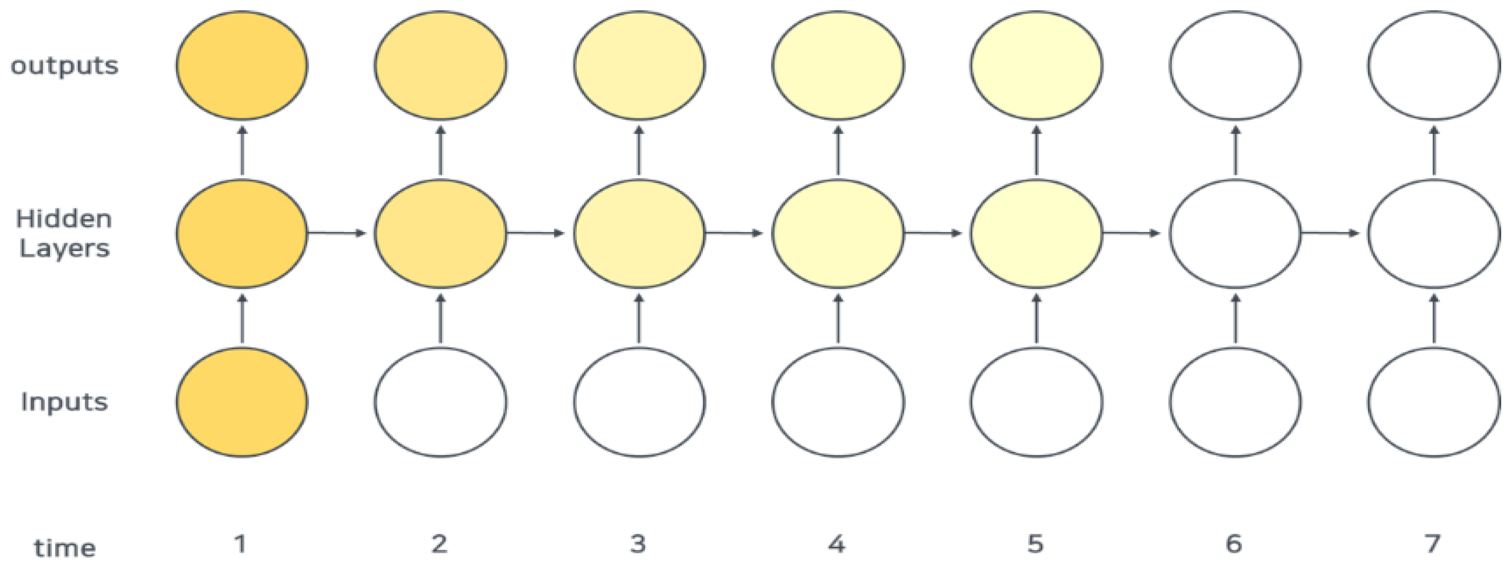
Deep learning methodologies consist of representative methods for processing time-series data, namely recurrent neural network (RNN) and long short-term memory (LSTM) methodologies. They are utilized to process time-series data and improve the prediction performance by reducing the likelihood of information loss by inputting data according to the time window in neural network operations. RNN is a deep learning algorithm in which the output values are fed back as inputs resulting in a repetition of the loops. This ensures consistent use of information. RNN is a network that considers past data and is mainly used for time-correlated data provided that all inputs and outputs are independent. As shown in Figure 1, the input to the network appears as an output value.
is a hidden state of the current state and is renewed after receiving a hidden state from the previous state. This has a deep learning network structure that emphasizes the flexibility of the model to accept inputs and outputs regardless of the length of the sequence in data.
However, the drawback of RNN is that the slope diminishes with an increase in time. This is known as the vanishing gradient problem in which various weights within a given neural network reduce the data update resulting in the discontinuation of learning in the neural network. Figure 2 depicts the gradient vanishing problem.
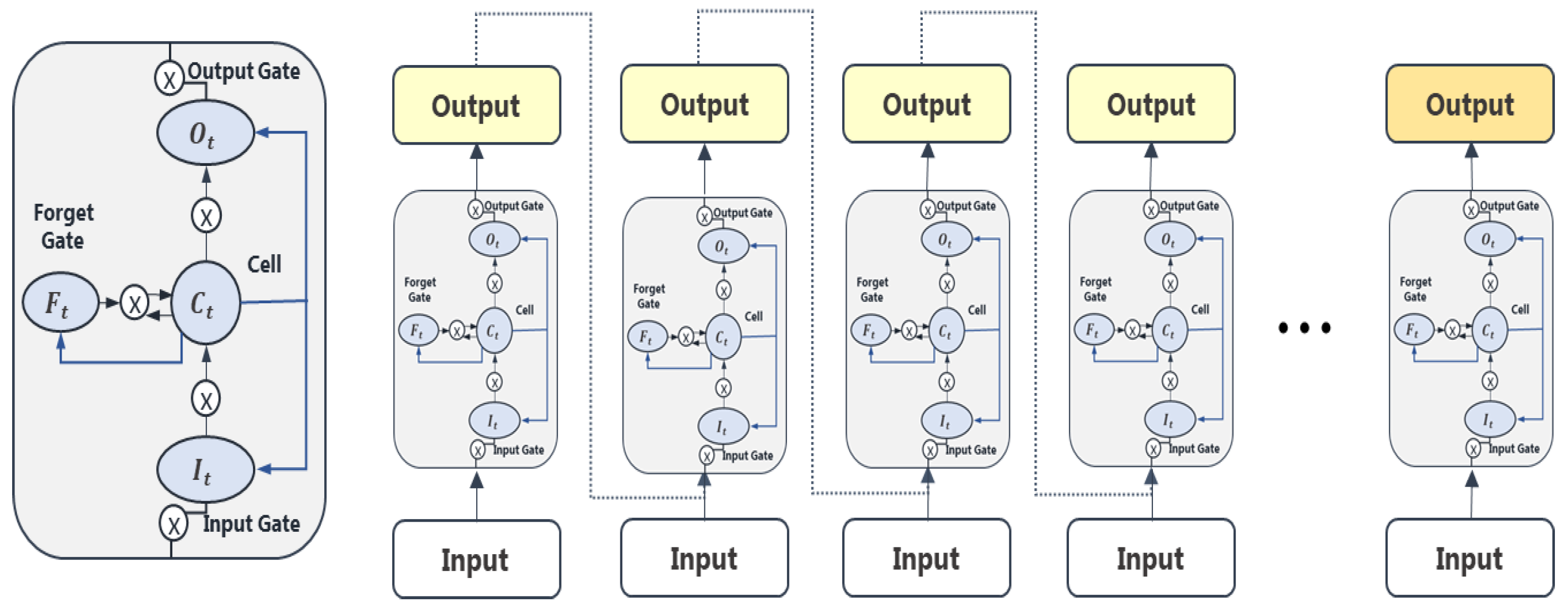
LSTM is an algorithm that improves the performance of the model by replacing the hidden layer of the RNN with memory blocks; it exhibits intensified performance in long-term memory through repeated information selection and removal of hidden networks. This addresses the vanishing gradient problem caused by distance when information in RNN is updated because it has the advantage of flexibly accepting input and output values of the network regardless of the length of the sequence.
The structure of LSTM comprises a series of “gates” unlike that of RNN (Figure 3). Gates are included in the memory blocks linked through each layer. They are identified as input, forget, and output gates, which can selectively allow the inputs to transfer information to output gates. The gates control the reading and writing of data, such as switches, and incorporate long-term memory into the model.
2.3. Sequential Models with Container Volume Prediction
Traditional time-series prediction exhibits good performance in short-term prediction; however, long-term prediction results rarely reflect unpredictable external economic situations [4]. With advances in technology and the use of various external variables in the prediction model to compensate for these limitations, there is a visible improvement in the performance; however, with this improvement, the problem of predicting the trend (up, steady, or down) of the volume is newly presented [6].
Comparative studies were conducted between the ARIMA model, a representative nonlinear forecasting model for container volume prediction of domestic ports, and a hybrid model obtained by combining the ARIMA model and an artificial neural network (ANN) model to enhance container volume prediction [10]. The results show that ANN and hybrid models exhibit better predictive performance than conventional ARIMA models. Based on these results, it was verified that the performance of deep learning-based models was better than that of existing traditional models.
Another study was conducted to compare deep learning and various time-series prediction models in the monthly container volume prediction of Singapore ports. It was noted that network LSTM models recorded the best performance [11]. Furthermore, we propose that multivariate LSTM neural networks using external variables perform better than the traditional time-series models.
In [12], RNNs and LSTMs were used to study daily container volume prediction based on deep learning to improve the efficiency of yard and ship loading plans at port terminals. In the LSTM–RNN model, the prediction error was approximately 12.39%, which was lower than that in human-based prediction. Hence, this study demonstrates that the performance of daily prediction of container volume based on deep learning using historical data is better than the empirical prediction by humans. This presented the current problem of relying on empirical decision-making in the port industry and highlighted the operational efficiency augmentation based on deep learning using time-series data [12].
The study of volume prediction at Busan port in Korea, indicated that the development of the port is closely related to national competitiveness and in fact, strengthens it; hence, accurate prediction of container volume is essential [4]. For this prediction, an LSTM model was used among the various deep learning models because trends and patterns of time-series data alone cannot represent variability due to rapid changes in the shipping and port logistics industry, such as economic market changes, financial crises, and variations in ship size. Thus, it was observed that the performance of volume prediction based on deep learning performs better than the existing SARIMA-based model.
The application of deep learning for volume prediction has resulted in improved performance over traditional statistical models. In addition, introducing external variables that are flexible to accept variability in volume and not limited to univariate prediction in utilizing deep learning cannot be overlooked.
3. Method
This section describes the data pre-processing technique followed by a time-series decomposition method. A flowchart of the proposed method is shown in Figure 4.
Exploration and verification of appropriate external variables are essential to predict the volume of loading containers at Busan port. This is done by utilizing the characteristics of time-series data and external variables. First, we checked the trend similarity and correlation with external variables with those of the container volume data. After selecting external variables with a correlation of 0.85, a VAR model is implemented for each external variable and volume. The VAR model is a regression model that considers both the past of the past and the past of relative data. In addition, it analyzes dynamic relationships between variables by estimating the relationships between all available time-series data without theoretical constraints. This model is also capable of executing simple predictions without considering the theoretical relationships between variables.
After selecting the external variables from the results of VAR model implementation, we performed time-series decomposition based on additive models of volume and each variable to improve the performance of deep learning prediction. We derived the predictions using a multivariate LSTM model for each decomposed time-series element including external variables. Finally, we compared the prediction performance of SARIMA, gated recurrent unit (GRU), bidirectional GRU, univariate LSTM, bidirectional LSTM, multivariate LSTM, and time-series decomposition-based multivariate LSTM. The key difference between GRU and LSTM is that GRU’s bag has two gates that are reset and update while LSTM has three gates that are input, output, and forget. GRU is less complex than LSTM because it has less number of gates. If the dataset is small then GRU is preferred otherwise LSTM for the larger dataset. For the bidirectional approach, the bidirectional approach algorithm can manage inputs in two ways, one from past to future and one from future to past, and this approach differs from unidirectional.
3.1. Data Analysis
The container data are time-series data composed of three elements: trend, seasonality, and residual information. Time-series data represent a set of sequentially determined datasets collected over a period. That is, time-series data indicate that data exist over a period of time. They usually depend on historical series up to a point in time when observed. This indicates that time-series data-based predictions analyze the observed historical data and apply the corresponding time-series prediction models [13]. In this study, we first conducted time-series decomposition to explore the features of the volume data. Volume data are characterized by additive models; the core components consist of trends, seasonality, and residuals. The following tables and figures illustrate the components of the time-series decomposition of container volume data. Each component of the container volume is listed in Table 1.
When time-series data consist of deterministic components proportional to the period, they are said to have trends. Trends in time-series data also affect testing and modeling. This is because the reliability of time-series models is relevant in properly identifying and processing trends over time.
Seasonality is characterized when time-series data show regular and predictable patterns according to the time period from the data. This characteristic of time-series data helps to improve the performance of modeling because the relationship between input and output variables improves when seasonal components of time-series data are identified and removed. In addition, seasonal definitions of time-series provide new information to improve the model performance.
Finally, the residuals represent the remaining components after trend and seasonality characteristics resulting from fluctuations in the time-series are removed from the time-series data. Residuals have no correlation; however, if a correlation exists, then the remaining information should be used in the prediction calculation. Furthermore, the mean of the residuals is zero. If the mean has a nonzero value, the prediction is prone to error.
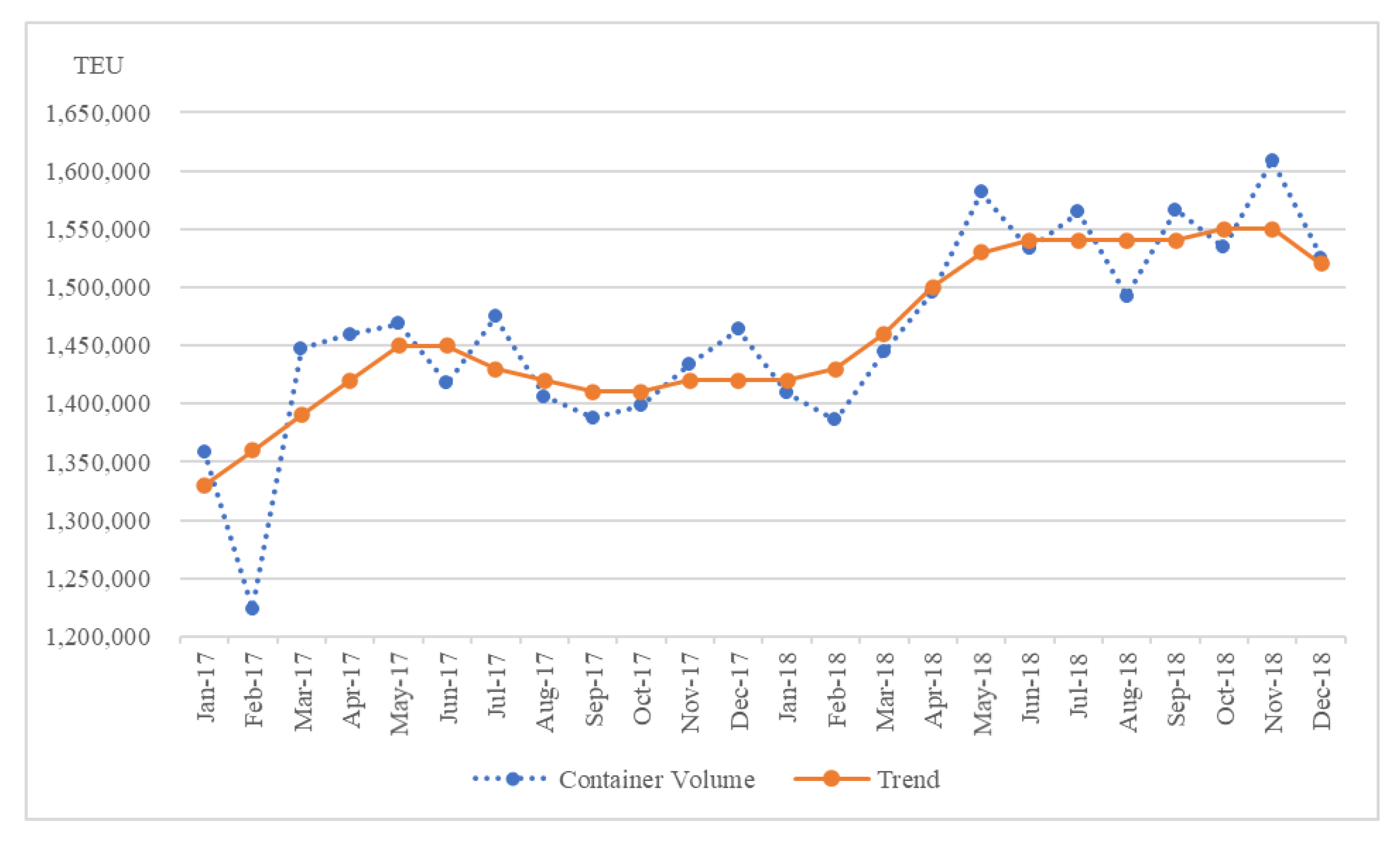
The historical records of loading container volume data at Busan Port that represent the volume figures and trends for 2017–2018 and 2019–2020 are different. Figure 5 represents a comparison of container volumes and trends for the years 2017–2018.
It can be observed that the gap between each line is negligible, and the trend is shown to some extent. Based on the time-series decomposition characteristics, we know that there is no significant variation in the value of the residuals among the time-series elements of the container volume. For seasonality, the same value is repeated based on the fourth quarter; hence, the deviation of the trend from the value of the container volume exhibits low error indicating that the value of the residual does not deviate significantly.
However, the container volume data and trends for the years 2019–2020 shown in Figure 6 indicate a different pattern from that shown in Figure 5 for the previous two years. Data from the volume itself indicate a sharp increase compared to the last two years; however, the trend over the past two years tends to be more modest. That is, the variation in the residuals of the volume increases with time. The residual standard deviation for 2017–2018 is 191.4 whereas that for 2019–2020 is 222.3. The inherent variability in container volume data increases with an increase in time. Furthermore, container volume data are particularly vulnerable to complexity and variability due to internal and external economic and environmental changes; hence, single variables alone have limitations in prediction performance.
3.2. Selection of External Variables
Various economic indicators can be applied to container volume forecasts. First, we chose from the various external variables presented in relevant studies and economic indicators that represent domestic economic fluctuations. Next, we implemented the VAR model to explore the influence of external variables on container volume prediction. The VAR model consists of a federated equation for the analysis of the effectiveness of a variable’s transient impact [13].
The selection criteria are correlations and trends that have proven influence according to previous research works [5,6]. The correlations and trends are considered together so that they can be applied in deep learning model applications and time-series decomposition methods.
The selected indicators are the manufacturing production index (MPI), industrial product index (IPI), import–export price (IEP), import–export weight (IEW), and consumer price index (CPI). However, the weight and price of exports and imports are used as a single variable by summing the two indicators. As shown in Table 2, the import–export weight and import–export price variables are highly correlated with each other, as well as with the container volume. Thus, we combined indicators by distinctive characteristics of them, which are weight and price. Based on our selection standards, five external variables were selected, which are represented by a correlation between the container volume data in Table 2. MPI, IPI, IEP, and IEW showed reasonable predictions in the short term (3 months), whereas long-term (6 months) prediction was limited in terms of accuracy improvement. As the duration of prediction increases, the prediction performance decreases simultaneously. However, only CPI, which has a high correlation and cointegration relationship, exhibited a performance with less than a mean absolute error (MAE) of 5 %; the other indicators did not show accurate predictions. Although CPI performed better in VAR model prediction, trend followability is an area of concern in container prediction.
3.3. Time-Series Decomposition with LSTM Model
This study presents a multivariate LSTM model utilizing time-series decomposition and external variables to improve the performance of container volume prediction. Time-series decomposition is a method executed to decompose each feature (trend, seasonality, and residual) that constitutes the time-series data to predict each element. Not only the container volume data set, but also external variables go through the same mechanism which decomposes each indicator by trend, seasonality, and residual. Since time series decomposing derives negative values from the residual component, thus we do decomposition for external variables as well. The multivariate LSTM model itself receives variables from multiple inputs. Thus, trend, seasonality, and residual of external variables are applied as multiple inputs with the decomposed container volume data. After training the model, we can eventually get values of each component (trend, seasonality, and residual), and sum each value to get the final prediction value.
The presence of the time-varying factor has a significant impact on the predictive model. As the market environment changes, most variables have a significant amount of noise. The qualitative and quantitative variables are used to predict variability increase, which is not reflected directly in the model [14]. To overcome this difficulty, each element is predicted by combining with an external variable; then, the predicted results are presented by summing the values of each predicted time-series characteristics. Because the size of the seasonal pattern does not significantly affect the size of the data, the additive model is applied for container volume data prediction.
First, we decompose the volume data according to the construction of the time-series data expressing it as a trend, seasonality, and residual and then combine it with five external variables’ decomposed components to represent the process. Container volume data are denoted as in Equation (3), and trend, seasonality, and residual in Equations (4)–(6), respectively. Note that Trend Tr, , and represent the values at time t, and n is the total number of data; that is, the total time duration.
According to the characteristics of combining trend, seasonality, and residuals of the data in the Addictive Model, the container volume can be expressed by the equation . After decomposing the time-series data in Equations (4)–(6), it is combined with the external variables. Because external variables also have characteristics of time-series, the execution of time-series decomposition is similar to that of container volume data. Then, it is combined with the volume data for each time point. For external variables, the decomposed values are prepared and thus, the trend decomposed of the mth external variable can be expressed as Equation (7). The seasonality and residuals of external variables are given in Equations (8) and (9).
Equations (7)–(9) show the expressions that represent a combination of five external variables with container volume time-series components. To derive the input matrices, we first combine with the external variables’ trend component
expressed in Equation (10). The elements in the first column of the combined matrix are the trend values of the container volume; the other columns are those of the external variables. Therefore, the number of columns in the matrix is m, where m is the number of external variables. Combined matrices for seasonality and residuals are computed that denote each component input as TI, SI, and RI, respectively.
In this study, we considered 12 months (n = 12) as the input for the prediction of six months. Finally, Equations (13)–(15) are used to derive the predictive values of the elements based on different multivariate LSTM models. The layers that constitute the LSTM model are constructed differently because the multivariate LSTM model exhibits different layers that are optimized according to trend, seasonality, and residual information. The output of the trend is also expressed as a vector with t elements where t is the length of the output periods.
The output list of predicted values (PV) as the final volume prediction can be obtained from the derived trends, seasonality, and residuals as shown in Equation (16).
Figure 7 represents the neural network architecture of time-series decomposition with the LSTM model for the proposed method.
To assess the performance of the proposed model and compare it with other methods, MAE and root mean squared error (RMSE), which are denoted in Equations (17) and (18), are used.
4. Experiments and Results
The computing environment was Windows 10 run on an RTX 2070 SUPER GPU and Python 3.7. The neural network models were configured using the Keras framework. Data from the Busan Port Authority’s shipping and port logistics analysis system were used to evaluate the effectiveness of the Busan Port loading container volume forecast proposed in this study. The loading container consists of import, export, and transfer; the container volume is aggregated based on monthly indicators. In this study, import, export, and transfer containers were combined to obtain the total loaded container volume
The original container volume data is stored monthly starting from March 2003 and extending to October 2020. External variables have the same time range as the container volume data. The train and test data are approximately split into 80% (March 2003~April 2018) and 20% (May 2018~October 2020), respectively. External variables follow the same split proportional rate as the container volume data. All variables are numerical data, and the summary is shown in Table 3.
When each time-series element is predicted in combination with an external variable as a multivariate model, the optimal layer exploration is initiated according to each element. The loss function used in the predictions was RMSE; moreover, an Adam optimizer was used. The optimizer instigates the search process for the value of hyperparameters such that the value of the loss function is minimized owing to the learning of neural network models. In this study, the optimal value is computed using an Adam optimizer by considering the direction of inertia after each calculation and previous situations together at every step. The trend and residual have different model layers and the model configuration is shown in Table 4.
Figure 8 shows a comparison between the actual and predicted values for six months from May to October 2020. In the figure, trend prediction reasonably follows the actual trend except in the last month.
For seasonality prediction, an accuracy of approximately 99% was recorded owing to the characteristic of representing the iteration of the same value based on the fourth quarter. Thus, we have a pattern of four values (–3320, −31,812, 25,311, and 9822) repeating continuously.
Finally, the residuals were predicted by combining the residuals of the external variables. As mentioned in Section 3.3, external variables should also be decomposed before inputting into the model. Table 5 is an example of a combination of residuals in a loaded container volume and those in external variables. Since residual components can provide negative values, which can affect the model, so all external variables are also represented in decomposed components.
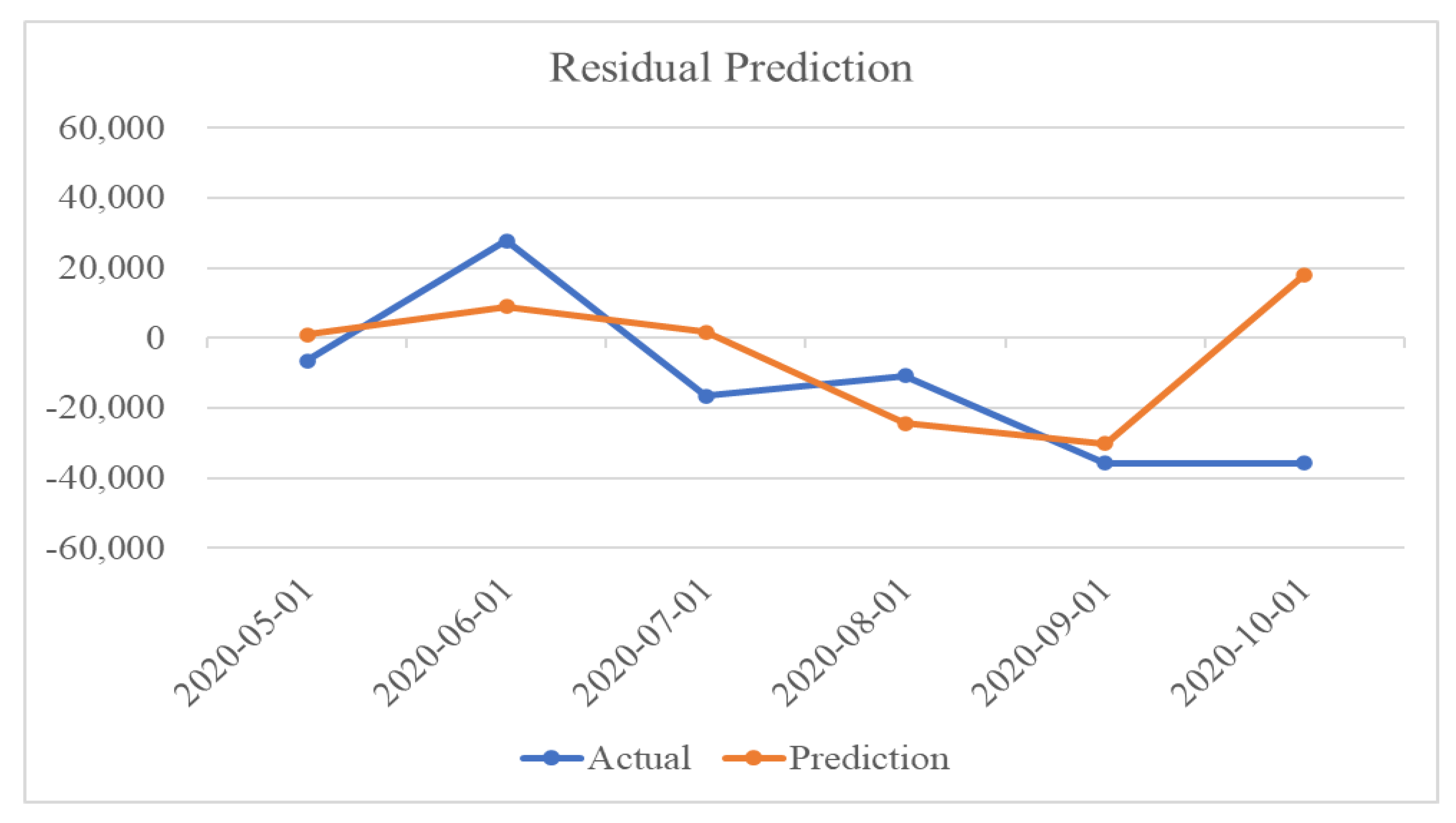
Residuals in container volume imply an increase in variability seen in the data problem; a decrease in residual prediction errors leads to a good prediction performance of container volume. In Figure 9, the residual prediction also shows reasonable results for six months, except for the last month.
Predictive results of trends and residuals show the characteristics of time-series decomposition. For October 2020, the predicted value of the trend was lower than the actual value, whereas the predicted value of the residuals was higher than the actual value. Owing to the additive characteristics in the additive model, the container volume shows that the error of each element is mitigated when the time-series element predictions are added at the end. The total prediction results are shown in Figure 10.
To compare the performance of the proposed model with the traditional model, experiments were conducted using various deep learning models, such as univariate LSTM, bidirectional LSTM, multivariate LSTM, GRU, and bidirectional GRUs. We compared the performance of the proposed model with the existing deep learning models and SARIMA-based prediction model, which is a traditional statistical methodology.
As the RMSE and MAPE evaluation metrics show that the error of the TD (Time-series Decomposition) model is the smallest, we can see that our method can bring the most effective forecasting performance among various prediction methods. In addition, by comparing the results of the unidirectional and bidirectional LSTM model, we can tell that bidirectional LSTM can perform better and unidirectional LSTM, which is denoted as univariate LSTM in Table 6. Furthermore, we could analyze the improvement of forecasting accuracy by importing external variables, which are manufacturing production index, industrial product index, import–export price, import–export weight, and consumer price index as a result of multivariate LSTM.
5. Discussion
The results indicate that time-series decomposition techniques can improve the predictive performance. The prediction errors shown in the trends and residuals were mitigated by each other in the additive model. Consequently, the proposed model has a positive effect not only on the predictive performance but also on the followability of trends (downward, steady, or upward). Thus, by predicting trends and residuals individually with external variables, we obtained better results.
However, besides the advantages of time-series decomposition, the problem of seasonality should always be considered in a timely manner. In this study, repetitive seasonality values were derived within a fixed period, 2003–2020; however, a longer time period with the addition of new data requires different seasonality values. Therefore, new seasonality values must be considered for a longer time period because there is a higher possibility of obtaining different values for seasonality.
In addition, the data used in our research were collected from a system called Port-MIS. However, the actual volume of the containers may not be the same as that of the system. The actual volume can be determined based on the terminal’s working history. This means that the information received in the system differs from the actual volume processed in the terminal. Thus, an error is generated from the data. Therefore, precise volume prediction may be possible based on the information of the actual container volume. Furthermore, the unit of measurement used in the experiment is a twenty-foot equivalent unit (TEU); however, the container has various TEU units that do not assure a precise index while aggregating or unifying the actual container volume from the system.
6. Conclusions and Future Research
In this study, we proposed a time-series decomposition method for a deep learning algorithm to improve the performance of container volume prediction. Owing to the nature of the time-series data, various external factors, such as the financial crisis and economic impact resulted in data instability. Hence, external variables have to be considered when predictive methods are used.
By applying a time-series decomposition method, it was observed that the prediction performance enhancement and trend prediction performance were improved. Thus, a prediction model along with decomposed variables has a positive effect on prediction performance.
Although time-series decomposition improves the performance, we do not consider the minor errors resulting from the decomposed values in this study. That is, after the decomposition, the sum of time-series components is not the same as the original container volume data. This minor difference must be handled appropriately, which is a prospective area of research. We plan to extend our study to container volume forecasting using a more fine-grained approach to obtain better prediction performance.
Author Contributions
Conceptualization E.L. and H.B.; Data curation, E.L., D.K. and H.B.; Formal analysis, E.L., H.B.; Methodology, E.L.; Investigation, H.B.; Supervision, H.B.; writing—original draft, E.L.; Writing—review & editing, D.K. and H.B.; project administration, H.B.; funding acquisition, H.B. All authors have read and agreed to the published version of the manuscript.
Funding
This research was supported by the 2021 Academic-Research Cooperation Program of the Korea Maritime Institute (KMI).
Institutional Review Board Statement
Not applicable.
Informed Consent Statement
Not applicable.
Conflicts of Interest
The authors declare no conflict of interest.
References
- Goodfellow, I.; Bengio, Y.; Courville, A. Deep Learning; MIT Press: London, UK; Cambridge, MA, USA, 2017. [Google Scholar]
- De la Rosa, E.; Yu, W.; Li, X. Nonlinear system modeling with deep neural networks and autoencoders algorithm. In Proceedings of the 2016 IEEE International Conference on Systems, Man, and Cybernetics (SMC), Budapest, Hungary, 9–12 October 2016; pp. 2157–2162. [Google Scholar] [CrossRef]
- Alsharif, M.; Younes, M.; Kim, J. Time series ARIMA model for prediction of daily and monthly average global SOLAR Radiation: The case study of Seoul, South Korea. Symmetry 2019, 11, 240. [Google Scholar] [CrossRef] [Green Version]
- Kim, D.; Lee, K. Forecasting the Container volumes of Busan port USING LSTM. J. Korea Port Econ. Assoc. 2020, 36, 53–62. [Google Scholar] [CrossRef]
- Intihar, M.; Kramberger, T.; Dragan, D. Container throughput forecasting using DYNAMIC factor analysis and Arimax Model. PROMET-Traffic. Transp. 2017, 29, 529–542. [Google Scholar] [CrossRef] [Green Version]
- Twrdy, E.; Batista, M. Modeling of container throughput in Northern Adriatic ports over the period 1990–2013. J. Transp. Geogr. 2016, 52, 131–142. [Google Scholar] [CrossRef]
- Velicer, W.; Fava, J. Time Series Analysis. In Handbook of Psychology; Weiner, I.B., Ed.; John Wiley and Sons: New York, NY, USA, 2003; Volume 2, pp. 581–606. [Google Scholar] [CrossRef]
- Ray, S.; Das, S.; Mishra, P.; Al Khatib, A. Time series SARIMA modelling and forecasting of monthly rainfall and temperature in the South Asian countries. Earth Syst. Environ. 2021, 5, 531–546. [Google Scholar] [CrossRef]
- Ghae, Y. Forecasting the Container throughput of the busan port using a seasonal multiplicative ARIMA model. Korea Port Econ. Assoc. 2013, 29, 1–23. [Google Scholar]
- Shin, C.; Jeong, S. A Study on Application of ARIMA and Neural Networks for Time Series Forecasting of Port Traffic. J. Navig. Port. Res. 2011, 35, 83–91. [Google Scholar] [CrossRef] [Green Version]
- Shankar, S.; Ilavarasan, P.; Punia, S.; Singh, S. Forecasting container throughput with long short-term memory networks. Ind. Manag. Data Syst. 2019, 120, 425–441. [Google Scholar] [CrossRef]
- Gao, Y.; Chang, D.; Chen, C.; Fang, T. Deep learning with long short-term memory recurrent neural network for daily container volumes of storage yard predictions in port. In Proceedings of the 2018 International Conference on Cyberworlds (CW), Singapore, 3–5 October 2018; pp. 427–430. [Google Scholar] [CrossRef]
- Du, S.; Li, T.; Yang, Y.; Horng, S.-J. Multivariate time series forecasting via attention-based encoder–decoder framework. Neurocomputing 2020, 388, 269–279. [Google Scholar] [CrossRef]
- Roh, T. Integration Model of Econometric Time Series for Volatility Forecasting. Korean Manag. Consult. Rev. 2013, 13, 313–340. [Google Scholar]
Figure 1.
Recurrent neural network.

Figure 2.
Gradient vanishing visualization.

Figure 3.
Memory block and long short-term memory structure.

Figure 4.
Flowchart of proposed method.

Figure 5.
Comparison of container volume and trends for the years 2017–2018 (x: date, y: TEU).

Figure 6.
Comparison of container volume and trends for the years 2019–2020 (x: date, y: TEU).

Figure 7.
Long short-term memory architecture for time-series decomposition.

Figure 8.
Trend prediction (x: data, y: TEU).

Figure 9.
Residual prediction (x: data, y: TEU).

Figure 10.
Multivariate LSTM prediction with time-series decomposition (x: date, y: TEU).


Table 1.
Container volume components visualization.
| Components | Graphs |
|---|---|
| Trend |  |
| Seasonality |  |
| Residual |  |
Table 2.
Correlation between container volume and external indicators.
| Volume | MPI | IPI | Export Weight | Import Weight | IEP | CPI | |
|---|---|---|---|---|---|---|---|
| Volume | 1 | 0.90 | 0.92 | 0.89 | 0.89 | 0.91 | 0.93 |
| MPI | 0.90 | 1 | 0.96 | 0.95 | 0.91 | 0.94 | 0.93 |
| IPI | 0.92 | 0.96 | 1 | 0.93 | 0.91 | 0.93 | 0.93 |
| Export Weight | 0.89 | 0.95 | 0.93 | 1 | 0.92 | 0.96 | 0.94 |
| Import Weight | 0.89 | 0.91 | 0.91 | 0.92 | 1 | 0.99 | 0.91 |
| IEP | 0.91 | 0.94 | 0.93 | 0.96 | 0.99 | 1 | 0.93 |
| CPI | 0.93 | 0.93 | 0.93 | 0.94 | 0.91 | 0.93 | 1 |
Table 3.
Summary statistics of the variables.
| Parameter | Container Volume | MPI | IPI | Import-Export Weight | CPI | Import-Export Price |
|---|---|---|---|---|---|---|
| Count | 212 | 212 | 212 | 212 | 212 | 212 |
| Mean | 1,113,716 | 89 | 91 | 93 | 84,078 | 72,457,330 |
| Standard Deviation | 279,131 | 16 | 13 | 9 | 13,084 | 19,434,553 |
| Minimum | 628,653 | 533 | 64 | 75 | 55,322 | 28,1899,734 |
| 25% | 838,584 | 75 | 81 | 84 | 71,439 | 56,477,292 |
| 50% | 1,129,280 | 96 | 94 | 97 | 86,925 | 77,572,986 |
| 75% | 1,353,759 | 105 | 102 | 101 | 93,748 | 89,170,656 |
| Maximum | 1,632,064 | 114 | 121 | 106 | 108,726 | 103,340,928 |
Table 4.
Model configuration.
| Hyper-Parameter | Trend | Residual |
|---|---|---|
| Recurrent layer Hidden units Gate activation Batch Normalization Dropout | 3 LSTM layer 200 of each layer Tanh - 20% of each layer | 3 LSTM layer 200 of each layer Tanh Each layer 20% of each layer |
| Wrapper layer Hidden units Activation | 1 Time Distributed layer # of prediction steps Sigmoid | 1 Time Distributed layer # of prediction steps Sigmoid |
| Loss function | MSE | MSE |
| Optimizer | Adam | Adam |
Table 5.
Residuals combination of container volume with external indicators.
| Volume Residual | MPI | IPI | Export Weight | Import Weight | CPI | Export Price | Import Price | |
|---|---|---|---|---|---|---|---|---|
| 03-Mar | 41,010.5 | 0.41 | 1.38 | 124.46 | 1421.21 | 0.54 | −248,245 | 632,178 |
| 03-Apr | 27,836.5 | 0.86 | −1.02 | 475.58 | −97.84 | 0.17 | 680,954 | −26,334 |
| 03-May | −25,667 | 0.29 | 0.90 | −821.10 | −731.66 | −0.10 | −103,564 | −62,941 |
| 03-Jun | 337,86.7 | 2.12 | 2.24 | 324.43 | −1847.70 | −0.13 | 608,408 | 257,613 |
Table 6.
Comparison of RMSE and MAPE for deep learning models.
| SARIMA | Univariate LSTM | Bidirectional LSTM | Multivariate LSTM | GRU | Bidirectional GRU | TD (Time-Series Decomposition) | |
|---|---|---|---|---|---|---|---|
| RMSE | 169,705 | 113,902 | 75,348 | 53,799 | 79,932 | 83,232 | 25,868 |
| MAPE | 22.14% | 18.10% | 14.02% | 13.24% | 14.75% | 15.26% | 10.95% |
Publisher’s Note: MDPI stays neutral with regard to jurisdictional claims in published maps and institutional affiliations. |
© 2021 by the authors. Licensee MDPI, Basel, Switzerland. This article is an open access article distributed under the terms and conditions of the Creative Commons Attribution (CC BY) license (https://creativecommons.org/licenses/by/4.0/).
Share and Cite
MDPI and ACS Style
Lee, E.; Kim, D.; Bae, H. Container Volume Prediction Using Time-Series Decomposition with a Long Short-Term Memory Models. Appl. Sci. 2021, 11, 8995. https://0-doi-org.brum.beds.ac.uk/10.3390/app11198995
AMA Style
Lee E, Kim D, Bae H. Container Volume Prediction Using Time-Series Decomposition with a Long Short-Term Memory Models. Applied Sciences. 2021; 11(19):8995. https://0-doi-org.brum.beds.ac.uk/10.3390/app11198995
Chicago/Turabian StyleLee, Eunju, Dohee Kim, and Hyerim Bae. 2021. "Container Volume Prediction Using Time-Series Decomposition with a Long Short-Term Memory Models" Applied Sciences 11, no. 19: 8995. https://0-doi-org.brum.beds.ac.uk/10.3390/app11198995
Note that from the first issue of 2016, this journal uses article numbers instead of page numbers. See further details here.