Sensitivity Analysis of Reliability of Low-Mobility Parallel Mechanisms Based on a Response Surface Method

Abstract

Kinematic accuracy is a crucial indicator for evaluating the performance of mechanisms. Low-mobility parallel mechanisms are examples of parallel robots that have been successfully employed in many industrial fields. Previous studies analyzing the kinematic accuracy analysis of parallel mechanisms typically ignore the randomness of each component of input error, leading to imprecise conclusions. In this paper, we use homogeneous transforms to develop the inverse kinematics models of an improved Delta parallel mechanism. Based on the inverse kinematics and the first-order Taylor approximation, a model is presented considering errors from the kinematic parameters describing the mechanism’s geometry, clearance errors associated with revolute joints and driving errors associated with actuators. The response surface method is employed to build an explicit limit state function for describing position errors of the end-effector in the combined direction. As a result, a mathematical model of kinematic reliability of the improved Delta mechanism is derived considering the randomness of every input error component. And then, reliability sensitivity of the improved Delta parallel mechanism is analyzed, and the influences of the randomness of each input error component on the kinematic reliability of the mechanism are quantitatively calculated. The kinematic reliability and proposed sensitivity analysis provide a theoretical reference for the synthesis and optimum design of parallel mechanisms for kinematic accuracy.

1. Introduction

A parallel robot has the advantages of high structural stiffness, high precision of both position and pose, low manufacturing and control cost, etc. Since Hunt proposed that the 6-DOF Stewart mechanisms could be used as robot mechanisms [1,2], the parallel mechanisms have gradually attracted increasing interest around the world. Kinematic reliability research for robots mainly focuses on evaluating the kinematic reliability and repetitive positioning accuracy of the robot mechanisms and making reasonable reliability predictions for kinematic accuracy of robots. Reliability sensitivity analysis can quantitatively calculate the influences of each random variable on the reliability, and then obtain the key factors and control the randomness of parameters to improve overall system reliability. The Delta parallel robot is one of the most practical low-mobility parallel robots in industry fields. The original Delta mechanism was proposed and patented by Clavel in Switzerland in 1998 [3,4]. Tsai proposed a simpler improved Delta parallel mechanism in 1995 [5,6,7]. Jaime Gallardo-Alvarado et al. analyzed the displacement, velocity and acceleration of a Delta-type robot by applying the screw theory [8]. Based on the concept of virtual power coefficients and pressure angles, Brinker et al. defined a single motion/force transmission index to evaluate the kinematic performance of the Delta parallel robot [9]. Lu et al. proposed an intelligent control scheme using self-learning interval type-2 fuzzy neural network (SLIT2FNN) for the trajectory tracking problem of a Delta robot [10]. Xu and Sun defined the stiffness matrix for mechanisms based on the Hessian matrix of its potential energy, and then established a new continuous stiffness mapping model for the Delta parallel mechanism [11]. Orsino et al. studied analytical mechanics approaches in the dynamic modelling of the Delta mechanism. Four modelling methods were analyzed and compared: One based on the Principle of Virtual Work, two based on Lagrange’s equations and one based on Kane’s formalism [12]. Kuo utilized the kineto-elasto-dynamics and the finite element method to perform a mathematical dynamic model of a Delta robot with flexible links [13]. In order to obtain the best dexterity over its workspace, Vitor Gaspar Silva, Mahmoud Tavakoli, and Lino Marques optimized the spatial 3-DOF Delta parallel manipulator with a floating-point genetic algorithm [14]. Belkacem Bounab proposed a multi-objective optimal design for the Delta robot based on kineto-elastostatic performances such as uniformity of the dexterity, largest regular workspace, highest global stiffness and reduced moving mass for the Delta robot [15]. Mazare and Taghizadeh presented an optimal design for the geometric parameters of 3-P2(US) Delta parallel mechanism using harmony search algorithm [16]. The research on the kinematic accuracy of serial and parallel mechanisms has attracted significant interest [17,18]. Tang et al. presented an error modeling methodology that enables the tolerance design and kinematic calibration of 3-RSS Delta mechanism. The sensitivity analysis and kinematic calibration were also carried out to investigate the influence of source errors on the pose accuracy [19,20]. By using a laser tracker as a measurement tool, Zhang et al. presented an iterative method to identify 18 geometric errors of the Delta parallel robot [21]. Ghazi et al. analyzed the kinematic accuracy of a 3-DOF Delta parallel manipulator via both Jacobian and geometric error models [22]. Dragos et al. researched the influence of dimensional deviations, kinematic joints clearances and input errors introduced by the actuator on the positioning accuracy of the 3-DOF Delta parallel robots [23,24,25]. Tian and Zhang Designed generalized parallel manipulators, and the position analysis of the GPM was carried out to evaluate the workspace and reveal the motion characteristics [26]. Chen et al. researched the actuator input selection and optimization of the parallel mechanism, and evaluated the motion stability of each actuator [27]; Amir et al. presented analytical approach for the dimensional synthesis of the 3-DOF Delta parallel robot for a prescribed workspace [28]. Li et al. conducted research on the kinematics and error analysis considering the parallelism error of the mechanism [29]. Shen et al. studied the influence of the variations related to the manipulator components and geometric parameters onto the kinematic accuracy by means of the variational method [30].

At present, the kinematic accuracy analysis of mechanisms is mainly focused on method involving the modeling of static position and pose errors. However, due to the dimensional deviation and the clearances caused by the manufacturing tolerances, driving errors associated with the actuators and the errors introduced by link masses and moment of inertia, random variables must be included in the mechanical system. Kinematic accuracy analysis of parallel mechanisms in the previous studies typically ignores the randomness of each input error resulting in imprecise conclusions.

The main contributions of this paper are as follows: (1) In the previous study, kinematic accuracy analysis of the improved Delta parallel mechanism usually ignores the randomness of each input error component. In this paper, a new evaluation and calculation method of kinematic reliability proposed consider the influence of the randomness of input errors making the error estimation more accurate and practical. (2) The response surface method was adopted to analyze the reliability sensitivity of the improved Delta parallel mechanism. Compared to the traditional reliability sensitivity analysis of the parallel mechanisms, the new method for reliability sensitivity analysis proposed in this paper is available even if the ultimate state function i.e., the real analytical response expression of the mechanical system is unknown.

2. Response Surface Method

The response surface methodology (RSM) was first proposed by Box and Wilson [31]. The method has been widely applied in the chemical, pharmaceutical, agricultural and mechanical engineering fields [31,32,33]. The idea underlying this method is the assumption that the real expression of Y is unknown, the relationship between the output response Y of the structural system and the random input parameter vector $x=\left(x_1{, x}_2,\cdots {, x}_{NR}\right)$ is described by a quadratic function with cross terms, as shown in Equation (1). The reasons why RSM was adopted to analyze reliability sensitivity are follows: (1) It can be used when the limit state function i.e., the real analytical response expression of the mechanical system is unknown. (2) This limit state function is a simple quadratic polynomial, which facilitates the calculation of variance and partial derivatives, and makes the calculation of reliability sensitivity straightforward. (3) The limit state function includes the information of the first, second and cross terms, which greatly improves the accuracy of the reliability sensitivity calculation.

The Ns input samples of the random parameter vector are obtained by certain sampling methods, while a group of output values $\left(y_1{, y}_2,\cdots {, y}_{Ns}\right)$ of the structural system are obtained by experimental design or numerical analysis based on the Ns input values. The unknown coefficients of the response surface function are determined by the least square method in regression analysis, thus the response surface function is derived, which is used to replace the real response expression of the structural system in the following work.

$$Y=C_0+{\displaystyle {\sum }_{i=1}^{N_R}{C}_i}{X}_i+{\displaystyle {\sum }_{i=1}^{N_R}}{\displaystyle {\sum }_{j=1}^{N_R}{C}_{ij}{X}_i}{X}_j$$

(1)

where: $C_0$,$C_i$,${ C}_{ij}$ ($i=1$, …, $N_R$;$j=i$, …, $N_R$) are unknown coefficients.

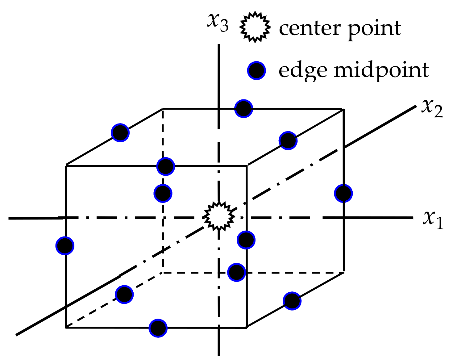
To obtain Ns samples of the random parameter vector, Box-Behnken sampling is used herein. This method not only reduces the number of samples but also improves the calculation accuracy of the response surface. According to the reference [31], three different level points are selected for each random variable, and then the center points and the edge midpoints are combined into samples according to certain rules. Figure 1 shows the Box-Behnken samples of three variables ($x_1{, x}_2{, x}_3$).

For a random variable $x_s$ which accords with arbitrarily distribution, its level value $p_n$ is calculated from Equation (2).

$${\displaystyle {\int }_{-\infty }^{x_s}f(x)dx=p_n},n=1,2,3$$

(2)

where: $f\left(x\right)$ is the distribution density function of random variables; $p_n$ are the random variable level, $p_1=0.01$, $p_2=0.50$, $p_3=0.99$.

For random variables of normal distribution

$$x_s=\mu +\sigma {\Phi }^{-1}\left(p_n\right)$$

(3)

where: $\mu$ is the mean; $\sigma$ is standard deviation; $\mathsf{\Phi }(°)$ is the standard normal distribution function.

The $Ns$ samples of random parameters are numerically calculated, then the $Ns$ corresponding output values $\left(y_1{, y}_2,\cdots {, y}_{Ns}\right)$ of the system response are obtained. These data are employed in a regression analysis using the least square method.

$$s={\displaystyle {\sum }_{i=1}^{N_s}{\epsilon }^2}={{\displaystyle {\sum }_{i=1}^{N_s}\left[C_0+{\displaystyle {\sum }_{i=1}^{N_R}{C}_i}{X}_i+{\displaystyle {\sum }_{i=1}^{N_R}}{\displaystyle {\sum }_{j=1}^{N_R}{C}_{ij}{X}_i}{X}_j\right]}}^2$$

(4)

where: Ns is the number of samples, $N_R$ is the number of random input variables and $\mathsf{\epsilon }$ is the error term.

To minimize the sum of each error term, then:

$$\left\{\begin{array}{c}\frac{\partial s}{\partial C_0}=0\\ \frac{\partial s}{\partial C_i}=0\\ \frac{\partial s}{\partial C_{ij}}=0\end{array}\right.\hspace{1em}i=1,2,\cdot \cdot \cdot ,N_R;\hspace{1em}j=1,2,\cdot \cdot \cdot ,N_R;$$

(5)

By solving Equation (5), the estimated values of the coefficients in Equation (1) can be calculated, and then the response surface function will be obtained.

3. Kinematics Analysis

3.1. Mechanism Description and Coordinate System

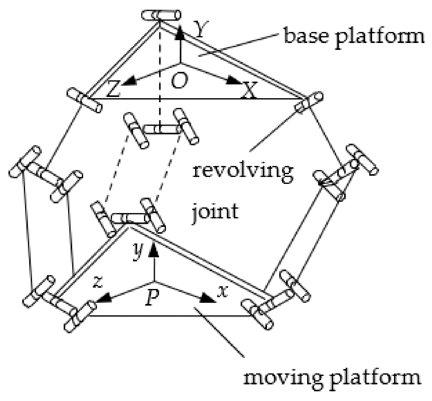
As shown in Figure 2, the improved Delta parallel mechanism without offsets consists of a moving platform, a base platform, and three identical branches connecting the two platforms. Each branch is connected by three revolute joints which are noncoplanar and a parallelogram mechanism. The improved Delta mechanism has three translational degrees of freedom.

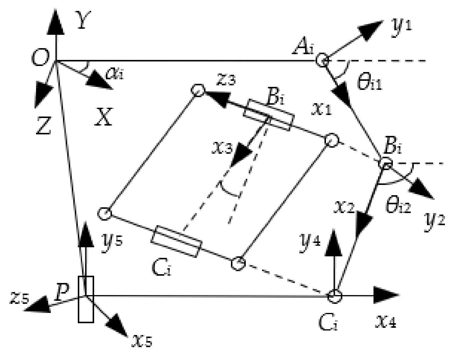
The kinematic sketch of any branch of the mechanism is shown in Figure 3. The rotation angle ${\theta }_{i1}$ (i = 1, 2, 3) of the three driving arms are the input motion. $A_i{B}_i{C}_i$(i = 1, 2, 3) is any branch, and P is the centroid of the moving platform. The global coordinate system ${\left(XYZ\right)}_O$ is located at the centroid O of the base platform, the x-axis points to ${OA}_1$, the $y$-axis is perpendicular to the surface of the platform, and the negative direction of the $y$-axis points to the moving platform. A local coordinate system is established for any equivalent linkage at each joint, as shown in Figure 3. The link parameters and the transformation matrices between adjacent coordinate systems are shown in

Table 1. Equivalent link parameters of improved Delta mechanism.

Equivalent Link	Local Coordinate	$\mathbf{Variable} {\mathbf{\theta }}_{\mathbf{i}}$	Transformation Matrix	Variation Range
1	${\left(\mathrm{xyz}\right)}_1$	${\theta }_{i1}$	${}^0{T}_1{=\mathrm{Rot}(y,\alpha }_i{\left)\mathrm{Trans}\right(x,r}_1\left)\mathrm{Rot}\right(z,-{\theta }_{i1})$	$20°–160°$
2	${\left(\mathrm{xyz}\right)}_2$	${\theta }_{i2}$	${}^1{T}_2{=\mathrm{Trans}(x,a)\mathrm{Rot}(z, \theta }_{i1}\left)\mathrm{Rot}\right(z, -{\theta }_{i2})$	$20°–160°$
3	${\left(\mathrm{xyz}\right)}_3$	${\theta }_{i3}$	${}^2{T}_3{=\mathrm{Rot}(y,\theta }_{i3})$	$\pm 40°$
4	${\left(\mathrm{xyz}\right)}_4$	-	${}^3{T}_4=\mathrm{Trans}(x,c)\mathrm{Rot}(y,-{\theta }_{i3}{\left)\mathrm{Rot}\right(z,\theta }_{i2})$	-
5	${\left(\mathrm{xyz}\right)}_5$	-	${}^4{T}_5=\mathrm{Trans}(x,-r_2\left)\mathrm{Rot}\right(y,-{\alpha }_i)$	-

Note:${ \mathrm{Trans}(x,r}_1)$ represents the homogeneous transform matrix for translating $r_1$ units vector along the x-axis of the local coordinate system; ${\mathrm{Rot}(y,\alpha }_i)$ represents the homogeneous transformation matrix of rotating the ${\alpha }_i$ angle about the y-axis of the local coordinate system; the others follow the same rule. Three identical branches correspond to i = 1, 2, and 3, respectively.

.

The locations of the revolute joints on the base platform and the moving platform of the mechanism are arranged in an equilateral triangle, and the radii of the circumcircles are $r_1$ and $r_2$, respectively. The length of each driving arm $A_i{B}_i$ is a, the length of each parallelogram mechanism $B_i{C}_i$ is c, and ${ \alpha }_i$ is the included angle between ${\mathrm{OA}O}_{\mathrm{i}}$ and x-axis of the global coordinate system. The input angle ${\theta }_{i1}$, the rotation angle ${\theta }_{i2}$ of each follower $B_i{C}_i$, and the swing angle ${\theta }_{i3}$ of each follower are shown in Figure 3.

3.2. Inverse Kinematics

The homogeneous transform ${}^0{T}_5$ of the coordinate system ${\left(xyz\right)}_5$ relative to the global coordinate system ${\left(XYZ\right)}_O$ is as follows:

$${}^0{T}_5={\displaystyle \prod _{i=1}^{i=5}{}^{i-1}{T}_i}$$

(6)

$${}^0{T}_5=\left[\begin{array}{cccc}1& 0& 0& x\\ 0& 1& 0& y\\ 0& 0& 1& z\\ 0& 0& 0& 1\end{array}\right]$$

(7)

where: (x, y, z) are the coordinates of point P, the origin of the end-effector coordinate system ${\left(xyz\right)}_5$ in the global coordinate system.

Equations (6) and (7) can be modified to obtain Equation (8):

$$Rot{(y,{\alpha }_i)}^{(-1)} {}^0{T}_{5}Rot{(y,-{\alpha }_i)}^{(-1)}$$

$$\left\{\begin{array}{l}{\theta }_{i3}=\arcsin (-t_z/c)\\ a\cos {\theta }_{i1}+b_0\cos {\theta }_{i2}=k_0\\ a\sin {\theta }_{i1}+b_0\sin {\theta }_{i2}=-t_y\end{array}\right. (i=1, 2, 3)$$

(8)

where:

$${{\displaystyle t}}_x=\cos {\alpha }_{i}x-\sin {\alpha }_{i}x,{{\displaystyle t}}_y=y;$$

$${{\displaystyle t}}_z=\cos {\alpha }_{i}z+\sin {\alpha }_{i}x;$$

$$b_0=c\cos {\theta }_{i3};$$

$$k_0=t_x-r_1+r_2;$$

${Rot(y,\alpha }_i{)}^{-1}$ is the inverse matrix of $Rot{\left({y,\alpha }_i\right)}^{ }$, and the others follow the same rule.

According to Equation (8),${\theta }_{i1} and{ \theta }_{i2}$ can be expressed as:

$${\theta }_{i1}=2\arctan \left(\frac{-t_{i1}\pm \sqrt{t_{i1}{}^2-4t_{i2}{t}_{i0}}}{2t_{i2}}\right)$$

(9)

$${\theta }_{i2}=2\arctan \left(\frac{-n_{i1}\pm \sqrt{n_{i1}{}^2-4n_{i2}{n}_{i0}}}{2n_{i2}}\right)$$

(10)

where:

$$t_{i2}=b_0^2-k_0^2-a^2-t_y^2-2a{k}_0$$

$$t_{i1}=-4a{t}_y{t}_{i0}=b_0^2-k_0^2-a^2-t_y^2+2a{k}_0$$

$$n_{i2}=b_0^2+k_0^2-a^2+t_y^2+2b_0{k}_0,n_{i1}=4b_0{t}_y$$

$$n_{i0}=b_0^2+k_0^2-a^2+t_y^2-2b_0{k}_0$$

The values of ${\theta }_{i1}$ is determined by Equation (9) and the inverse kinematics is completed. Moreover, ${\theta }_{i2}$ and ${ \theta }_{i3}$ are obtained from Equations (10) and (8). Typically, there are two sets of solutions corresponding to ${\theta }_{i1}$ and ${\theta }_{i2}$. According to the rule of “continuous variation” of joint rotation angle, when the initial position and posture of the mechanism are given, the unique function expressions of ${\theta }_{i1}$ and ${\theta }_{i2}$ are easily determined from Equations (9) and (10).

4. Error Modeling

The error sources of the mechanism are as follows: (1) the deviation between the actual geometrical parameters and the original design values caused by manufacturing and installation; (2) clearance errors associated with revolute joints; (3) the driving error. At any time, there is the deviation $\Delta {\theta }_{i1}$ between the actual rotation angle and the theoretical value from the actuator failing to drive the rotating arm $A_i{B}_i$ to the desired angle. The deviation $\Delta {\theta }_{i1}$ is called the driving error. (i = 1, 2, 3)

By solving Equations (6) and (7), x, y and z can be expressed as:

$$\left\{\begin{array}{l}x=-c\sin {\theta }_{i3}\sin {\alpha }_i+r_1\cos {\alpha }_i-r_2\cos {\alpha }_i\\ \hspace{1em}+a\cos {\theta }_{i1}\cos {\alpha }_i+c\cos {\theta }_{i2}\cos {\theta }_{i3}\cos {\alpha }_i\\ y=-a\sin {\theta }_{i1}-c\sin {\theta }_{i2}\cos {\theta }_{i3}\\ z=-c\sin {\theta }_{i3}\cos {\alpha }_i-r_1\sin {\alpha }_i+r_2\sin {\alpha }_i\\ \hspace{1em}-a\cos {\theta }_{i1}\sin {\alpha }_i-c\cos {\theta }_{i2}\cos {\theta }_{i3}\sin {\alpha }_i\end{array}\right. (i=1, 2, 3)$$

(11)

4.1. Geometric Parameters Errors

On each branch of the mechanism, the first-order Taylor approximation is utilized to calculate the position error of the end-effector at any time caused by the geometric parameters errors:

$$\left\{\begin{array}{l}\Delta x^0={\displaystyle \sum _{i=1}^3(k{x}_{1i}\Delta r_{1i}+k{x}_2{}_i\Delta r_{2i}+k{x}_3{}_i\Delta a_i}+k{x}_{4i}\Delta c_i+k{x}_5{}_i\Delta {\alpha }_i)\\ \Delta y^0={\displaystyle \sum _{i=1}^3(k{y}_1{}_i\Delta a_i+k{y}_{2i}\Delta c_i)}\\ \Delta z^0={\displaystyle \sum _{i=1}^3(k{z}_{1i}\Delta r_1{}_i+k{z}_2{}_i\Delta r_2{}_i+k{z}_3{}_i\Delta a_i}+k{z}_{4i}\Delta c_i+k{z}_{5i}\Delta {\alpha }_i)\end{array}\right. (i=1, 2, 3)$$

(12)

where: $\Delta r_{i1}$, $\Delta r_{i2}$, $\Delta a_i$, $\Delta c_i$ are the corresponding geometric parameters errors on the branch i (i = 1, 2, 3);$\Delta {\alpha }_i$ is the deviation between the actual locations and the theoretical values of the corresponding branches i (i = 1, 2, 3), and

$$k{x}_{1i}=\cos {\alpha }_i,k{x}_{2i}=-\cos {\alpha }_i,k{x}_{3i}=\cos {\alpha }_i\cos {\theta }_{i1};$$

$$k{x}_{4i}=\cos {\alpha }_i\cos {\theta }_{i2}\cos {\theta }_{i3}-\sin {\theta }_{i3}\sin {\alpha }_i;$$

$$k{x}_{5i}=-r_{i1}\sin {\alpha }_i+r_{i2}\sin {\alpha }_i-a_i\cos {\theta }_{i1}\sin {\alpha }_i-c_i\cos {\theta }_{i2}\cos {\theta }_{i3}\sin {\alpha }_i-c_i\sin {\theta }_{i3}\sin {\alpha }_i;$$

$$k{y}_{1i}=\sin {\theta }_{i1},k{y}_{1i}=\sin {\theta }_{i2}\cos {\theta }_{i3};$$

$$k{z}_{1i}=-\sin {\alpha }_i,k{z}_{2i}=\sin {\alpha }_i,k{z}_{3i}=-\cos {\theta }_{i1}\sin {\alpha }_i;$$

$$k{z}_{4i}=-\sin {\alpha }_i\cos {\theta }_{i2}\cos {\theta }_{i3}-\sin {\theta }_{i3}\sin {\alpha }_i;$$

$$k{z}_{5i}=-r_{i1}\cos {\alpha }_i+r_{i2}\cos {\alpha }_i-a_i\cos {\theta }_{i1}\cos {\alpha }_i-c_i\cos {\theta }_{i2}\cos {\theta }_{i3}\cos {\alpha }_i+c_i\sin {\theta }_{i3}\sin {\alpha }_i$$

4.2. Clearance Errors of Revolute Joints

In this paper, only the clearance errors of the revolute joints between the base platform and the driving arms are considered. According to the “effective length theory” [34], the end-effector position errors caused by the radial clearance errors of revolute joints are obtained as:

$$\left\{\begin{array}{l}\Delta x^R={\displaystyle \sum _{i=1}^3\cos {\theta }_{i1}\cos {\alpha }_i\Delta R_{ei}}\\ \Delta y^R=-{\displaystyle \sum _{i=1}^3\sin {\theta }_{i1}\Delta R_{ei}}\\ \Delta z^R=-{\displaystyle \sum _{i=1}^3\cos {\theta }_{i1}\sin {\alpha }_i\Delta R_{ei}}\end{array}\right.$$

(13)

where: $\Delta R_{ei}$ is the radial clearance errors of the revolving joints between the base platform and the driving arms on the branch i.

4.3. Driving Errors

From Equation (9), the three input angles ${\theta }_{11}$, ${\theta }_{21}$ and ${\theta }_{31}$ are the functions of coordinate value (x, y, z) of the origin P in the end-effector coordinate system ${\left(xyz\right)}_5$ at any time respectively. The functions ${\theta }_{11}{=f}_1(x,y,z)$, ${ \theta }_{21}{=f}_2(x,y,z)$ and ${\theta }_{31}{=f}_3(x,y,z)$, are expanded using the first-order Taylor approximation at their designed values respectively:

$$\Delta {\theta }_i{}_1=\frac{\partial f_i}{\partial x}\Delta x+\frac{\partial f_i}{\partial y}\Delta y+\frac{\partial f_i}{\partial z}\Delta z (i=1, 2, 3)$$

(14)

Therefore,

$$\left[\begin{array}{c}\Delta {\theta }_{11}\\ \Delta {\theta }_{21}\\ \Delta {\theta }_{31}\end{array}\right]=\left[\begin{array}{c}\partial f_i\\ \partial q\end{array}\right]\left[\begin{array}{c}\Delta x\\ \Delta y\\ \Delta z\end{array}\right] (q=x,y,z)$$

(15)

where: $\left[\begin{array}{c}\partial f_i\\ \partial q\end{array}\right]=\left[\begin{array}{ccc}\frac{\partial f_1}{\partial x}& \frac{\partial f_1}{\partial y}& \frac{\partial f_1}{\partial z}\\ \frac{\partial f_2}{\partial x}& \frac{\partial f_2}{\partial y}& \frac{\partial f_2}{\partial z}\\ \frac{\partial f_3}{\partial x}& \frac{\partial f_3}{\partial y}& \frac{\partial f_3}{\partial z}\end{array}\right]—\mathrm{Jacobian} \mathrm{Matrix} \mathrm{of} \mathrm{the} \mathrm{robot};$

${[\Delta {\theta }_{11},\Delta {\theta }_{21},\Delta {\theta }_{31}]}^T$ are the error vector of three input angles; ${\left[\Delta x,\Delta y,\Delta z\right]}^T$ are the position error vector of the end-effector.

The two sides of Equation (15) are simultaneously left multiplied by the inverse of the Jacobian matrix ${\left[\begin{array}{c}\partial f_i\\ \partial q\end{array}\right]}^{-1}$ of the robot:

$$\left[\begin{array}{c}\Delta x\\ \Delta y\\ \Delta z\end{array}\right]={\left[\begin{array}{c}\partial f_i\\ \partial q\end{array}\right]}^{-1}\left[\begin{array}{c}\Delta {\theta }_{11}\\ \Delta {\theta }_{21}\\ \Delta {\theta }_{31}\end{array}\right]$$

(16)

The position errors of the end-effector caused by the driving errors are:

$$\Delta q^D={\displaystyle \sum _{i=1}^{3}K{q}_i\Delta {\theta }_{i1}}(i=1,2,3, q=x,y,z)$$

(17)

where: ${Kq}_i$ are the corresponding elements in the inverse matrix of Jacobian matrix.

Suppose that the total errors of the end-effector in the x, y, z directions are the linear addition of the three kinds of position errors caused by geometric parameters errors, clearance errors of revolute joints, and driving errors:

$$\Delta q=\Delta q^O+\Delta q^R+\Delta q^D={\displaystyle \sum K{q}_s\Delta s} (q=x,y,z)$$

(18)

where: ${Kq}_s$ is the error transfer coefficient of the corresponding original error Δs, whose numerical values are generally determined by the configurations of the mechanism as well as the nominal dimensions of the structural parameters such as a, c, $r_1$ etc.

5. Kinematic Reliability Analysis

One goal of kinematic reliability analysis is to obtain the probability that the displacement, velocity and acceleration of the end-effector of any one mass-produced robot/mechanism according to a design blueprint fall into the allowable accuracy range during the design process. Based on kinematic reliability and its sensitivity analysis, this paper aims to find out the crucial indicator for evaluating the performance of mechanisms to improve the kinematic reliability of the robot.

• Assume that the geometric parameters errors, the clearance errors of revolute joints, and the driving errors (at any time) are independent of each other and that each error has a normal distribution. From Equation (18), the position errors of the robot end-effector obey the normal distribution in the x, y, and z directions at any time. The mean and standard deviation are shown as Equations (19) and (20).

  $${\mu }_s={\displaystyle \sum _{i=1}^{n}K{q}_{si}{\mu }_{si}}$$

  (19)

  $${\sigma }_s=\sqrt{{\displaystyle \sum _{i=1}^{n}K{q}_{si}^2{\sigma }_{si}^2}}$$

  (20)

  where: ${\mu }_{si},{\sigma }_{si}$ are the mean and standard deviation of each original input error respectively.

Referring to the definition of kinematic accuracy reliability as used in traditional mechanisms, the kinematic reliability of the parallel mechanism is defined as follows:

$$R=P({\epsilon }_1<\Delta q<{\epsilon }_2)=\Phi (\frac{{\epsilon }_2-{\mu }_s}{{\sigma }_s})-\Phi (\frac{{\epsilon }_1-{\mu }_s}{{\sigma }_s})$$

(21)

where: Φ(•) is the standard normal distribution function; and ${\epsilon }_2{, \epsilon }_1$ are upper and lower limits of the allowable limit errors.

The position error in the combined direction is

$$f(S)=\sqrt{\Delta x^2+\Delta y^2+\Delta z^2}$$

(22)

The mean and variance of the total position errors are approximated by the moment method from Equations (23) and (24), and the distribution of the total position errors can be determined by the Monte Carlo method [35,36].

$$E\left(\Delta \right)=f({\mu }_{s1},{\mu }_{s2},\cdot \cdot \cdot ,{\mu }_{sn})+\frac{1}{2}{\displaystyle \sum {}_{i=1}^n}\frac{{\partial }^{2}f(s)}{\partial s_i^2}\left|{}_{s=u}\right.\cdot {\sigma }_{si}^2$$

(23)

$$D(\Delta )={{\displaystyle {\sum }_{i=1}^n\left(\frac{\partial f(s)}{\partial s_i}\left|{}_{s=\mu }\right.\right)}}^2\cdot {\sigma }_{si}^2$$

(24)

where: $s_i$ is the independent random variable of each original input error.

2.

It is assumed that the discrete distribution data (or the distribution law) of each original input error is known. According to the Monte Carlo method, assign a value for random variable in the error source. Then a sampled value of Δq or f(S) can be obtained from Equation (18) or Equation (22). The multiple sampled values then used to create a frequency histogram. Furthermore, parameter estimation and hypothesis testing of the distribution type of Δq or f(S) are now completed. As such, the kinematic reliability of the mechanism in the x, y, z directions or in the combined direction based on the distribution function can now be calculated.

6. Sensitivity Analysis of Kinematic Reliability

6.1. Formulate the Limit State Function of the Position Errors in the Combined Direction Based on Response Surface Method

According to Equation (18), the calculation of the output position errors of the mechanism in the x, y, z directions are based on the approximate solution of the linear addition of the slight errors. From Equations (12) and (14), the calculation of the output position errors of the mechanism are completed by using the first-order Taylor approximation at the theoretical value of the random variable of each input error when the dimensional errors and driving errors are taken into account. The above factors result in a lack of precision in the calculation. Moreover, the limit state function is unknown. Therefore, the explicit limit state function of the mechanism output position error is established by applying the response surface method, and the sensitivity of kinematic reliability to the randomness of each input error is analyzed based on this function.

According to the Box-Behnken sampling, when the number of variables is greater than 3, the required samples are obtained by the combination of two-level factorial design and incomplete block design [31]. Similarly, the permutations and combinations of 12 variables $\left(x_1{, x}_2,\cdots {, x}_{12}\right)$ are obtained as shown in Equation (25) by Box-Behnken sampling. Meanwhile, 192 edge midpoints and 12 center points are obtained shown in Appendix B.

$$\begin{array}{c}\begin{array}{cccccccccccc}{\mathit{x}}_1& {\mathit{x}}_2& {\mathit{x}}_3& {\mathit{x}}_4& {\mathit{x}}_5& {\mathit{x}}_6& {\mathit{x}}_7& {\mathit{x}}_8& {\mathit{x}}_9& {\mathit{x}}_{10}& {\mathit{x}}_{11}& {\mathit{x}}_{12}\end{array}\\ \left[\begin{array}{cccccccccccc}\pm 1& \pm 1& 0& 0& \pm 1& 0& \pm 1& 0& 0& 0& 0& 0\\ 0& \pm 1& \pm 1& 0& 0& \pm 1& 0& \pm 1& 0& 0& 0& 0\\ 0& 0& \pm 1& \pm 1& 0& 0& \pm 1& 0& \pm 1& 0& 0& 0\\ 0& 0& 0& \pm 1& \pm 1& 0& 0& \pm 1& 0& \pm 1& 0& 0\\ 0& 0& 0& 0& \pm 1& \pm 1& 0& 0& \pm 1& 0& \pm 1& 0\\ 0& 0& 0& 0& 0& \pm 1& \pm 1& 0& 0& \pm 1& 0& \pm 1\\ \pm 1& 0& 0& 0& 0& 0& \pm 1& \pm 1& 0& 0& \pm 1& 0\\ 0& \pm 1& 0& 0& 0& 0& 0& \pm 1& \pm 1& 0& 0& \pm 1\\ \pm 1& 0& \pm 1& 0& 0& 0& 0& 0& \pm 1& \pm 1& 0& 0\\ 0& \pm 1& 0& \pm 1& 0& 0& 0& 0& 0& \pm 1& \pm 1& 0\\ 0& 0& \pm 1& 0& \pm 1& 0& 0& 0& 0& 0& \pm 1& \pm 1\\ \pm 1& 0& 0& \pm 1& 0& \pm 1& 0& 0& 0& 0& 0& \pm 1\\ 0& 0& 0& 0& 0& 0& 0& 0& 0& 0& 0& 0\end{array}\right]\end{array}$$

(25)

According to the above sample points, the unknown coefficients of the response surface function are determined by the least square method in regression analysis, thus the response surface function is determined (Equation (1)) and used to replace the real response expression of the structural system in the following work.

6.2. Kinematic Reliability of the Mechanism in the Combined Direction

Assume that Y in Equation (1) is the output position error of the improved Delta parallel mechanism in the combined direction, and U is the maximum allowable limit of the error, so the limit state function is

$$g(x)=U-Y=U-\left(C_0+{\displaystyle {\sum }_{i=1}^{N_R}{C}_i}{X}_i+{\displaystyle {\sum }_{i=1}^{N_R}}{\displaystyle {\sum }_{j=1}^{N_R}{C}_{ij}{X}_i}{X}_j\right)$$

(26)

The limit state function represents two states of the output position error of the mechanism in the combined direction:

$$\left\{\begin{array}{c}g(x)<0 \mathrm{failure} \mathrm{state};\\ g(x)>0 \mathrm{safe} \mathrm{state};\end{array}\right.$$

In Equation (26), the random parameters are independent of each other, and the mean matrix and variance matrix are $\mu =\left({\mu }_1{, \mu }_2,\cdots {, \mu }_{NR}\right){ \mathrm{and} D=(D}_1{, D}_2,\cdots {, D}_{NR})$, respectively,

so:

$$E\left(X_i^2\right)=E^2\left(X_i\right)+D\left(X_i\right)={\mu }_i^2+D_i$$

(27)

$$E(X_i{X}_j)=E(X_i)E(X_j)={\mu }_i{\mu }_j$$

(28)

$$D(X_i^2)=4{\mu }_i^2{D}_i+2D_i$$

(29)

$$D(X_i{X}_j)={\mu }_i^2{D}_j+{\mu }_j^2{D}_i+D_i{D}_j$$

(30)

Therefore,

$$E\left(g(x)\right)={\mu }_g({\mu }_1,{\mu }_2,\cdot \cdot \cdot ,{\mu }_{NR},D_1,D_2,\cdot \cdot \cdot ,D_{NR})$$

(31)

$$D\left(g(x)\right)=D_g({\mu }_1,{\mu }_2,\cdot \cdot \cdot ,{\mu }_{NR},D_1,D_2,\cdot \cdot \cdot ,D_{NR})$$

(32)

The reliability index is defined as

$$\beta =\frac{{\mu }_g}{\sqrt{D_g}}$$

(33)

If the $g\left(x\right)$ obeys the normal distribution, the reliability can be expressed as

$$R=\Phi (\beta )$$

(34)

Note that the Monte Carlo method can be used to calculate reliability if $g\left(x\right)$ has an arbitrary distribution [37].

6.3. Reliability Sensitivity Analysis

The sensitivity of the kinematic reliability of the mechanism in the combined direction to the mean matrix μ and variance matrix D of each input error random variable are

$$\frac{\partial R}{\partial {\mu }^T}=\frac{\partial R}{\partial \beta }\left(\frac{\partial \beta }{\partial {\mu }_g}\frac{\partial {\mu }_g}{\partial {\mu }^T}+\frac{\partial \beta }{\partial D_g}\frac{\partial D_g}{\partial {\mu }^T}\right)$$

(35)

$$\frac{\partial R}{\partial D^T}=\frac{\partial R}{\partial \beta }\left(\frac{\partial \beta }{\partial {\mu }_g}\frac{\partial {\mu }_g}{\partial D^T}+\frac{\partial \beta }{\partial D_g}\frac{\partial D_g}{\partial D^T}\right)$$

(36)

where:

$$\left\{\begin{array}{l}\frac{\partial R}{\partial \beta }=\phi (\beta );\hspace{1em}\frac{\partial \beta }{\partial {\mu }_g}=\frac{1}{\sqrt{D_g}}\\ \frac{\partial \beta }{\partial D_g}=-\frac{{\mu }_g}{2}{\mathit{D}}_{\mathit{g}}^{-\frac{3}{2}}\\ \frac{\partial {\mu }_g}{\partial {\mu }^T}={\left[\frac{\partial {\mu }_g}{\partial {\mu }_1}, \frac{\partial {\mu }_g}{\partial {\mu }_2},\cdots , \frac{\partial {\mu }_g}{\partial {\mu }_{NR}}\right]}^T\\ \frac{\partial {\mu }_g}{\partial D^T}={\left[\frac{\partial {\mu }_g}{\partial D_1}, \frac{\partial {\mu }_g}{\partial D_2},\cdots , \frac{\partial {\mu }_g}{\partial D_{NR}}\right]}^T\\ \frac{\partial D_g}{\partial {\mu }^T}={\left[\frac{\partial D_g}{\partial {\mu }_1}, \frac{\partial D_g}{\partial {\mu }_2},\cdots , \frac{\partial D_g}{\partial {\mu }_{NR}}\right]}^T\\ \frac{\partial D_g}{\partial D^T}={\left[\frac{\partial D_g}{\partial D_1}, \frac{\partial D_g}{\partial D_2},\cdots , \frac{\partial D_g}{\partial D_{NR}}\right]}^T\end{array}\right.$$

(37)

Recall that: in this paper, the response surface function as shown in Equation (1) is used to approximate the real response of the system. Although the response surface function includes the information of the first, second and cross terms described in Equation (1) of the input variables, sensitivity analysis uses the linear realization of input variables essentially to dilute the effects of nonlinearity and coupling errors caused by parallel mechanisms. Therefore, sensitivity analysis on reliability in this paper is mainly based on the above assumptions for theoretical research.

7. Numerical Examples

The structural parameters of an improved Delta parallel mechanism are $r_{i1}{=200 \mathrm{mm}, r}_{i2}{=200 \mathrm{mm}, a}_i{=200 \mathrm{mm}, c}_i{=400 \mathrm{mm}, \alpha }_{1 }{=0°, \alpha }_2{=120°, \alpha }_{3 }=240°$(i = 1, 2, 3). The initial posture is: ${\theta }_{i1}=40{.54°, \theta }_{i2}=112{.33°, \theta }_{i3}=0°$(i = 1, 2, 3). The trajectory of point P is: $x=-30\sin \left(120°t\right), y =-500-20t, z=-30\cos \left(120°t\right)+30$, and the time is 3 s. Assuming that all the original errors are independent of each other and have a normal distribution with mean and standard deviations shown in

Table 2. Mean and standard deviation of original input errors.

Original Input Errors (i = 1, 2, 3)	Mean μ	Standard Deviation σ
Radius error of moving platform $\Delta r_{i2}$/mm	0.02	0.01
Length error of driving arm $\Delta a_i$/mm	0.06	0.0067
Clearance error of revolute pair $\Delta {\phi }_i$/mm	0.10	0.01
Driving error at any time $\Delta {\theta }_{i1}$/rad	0.03	0.1173

.

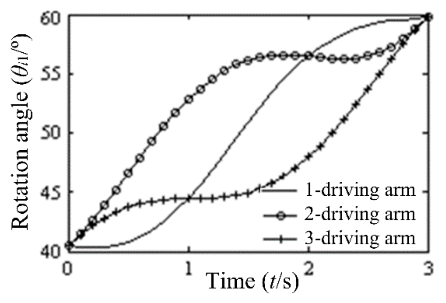
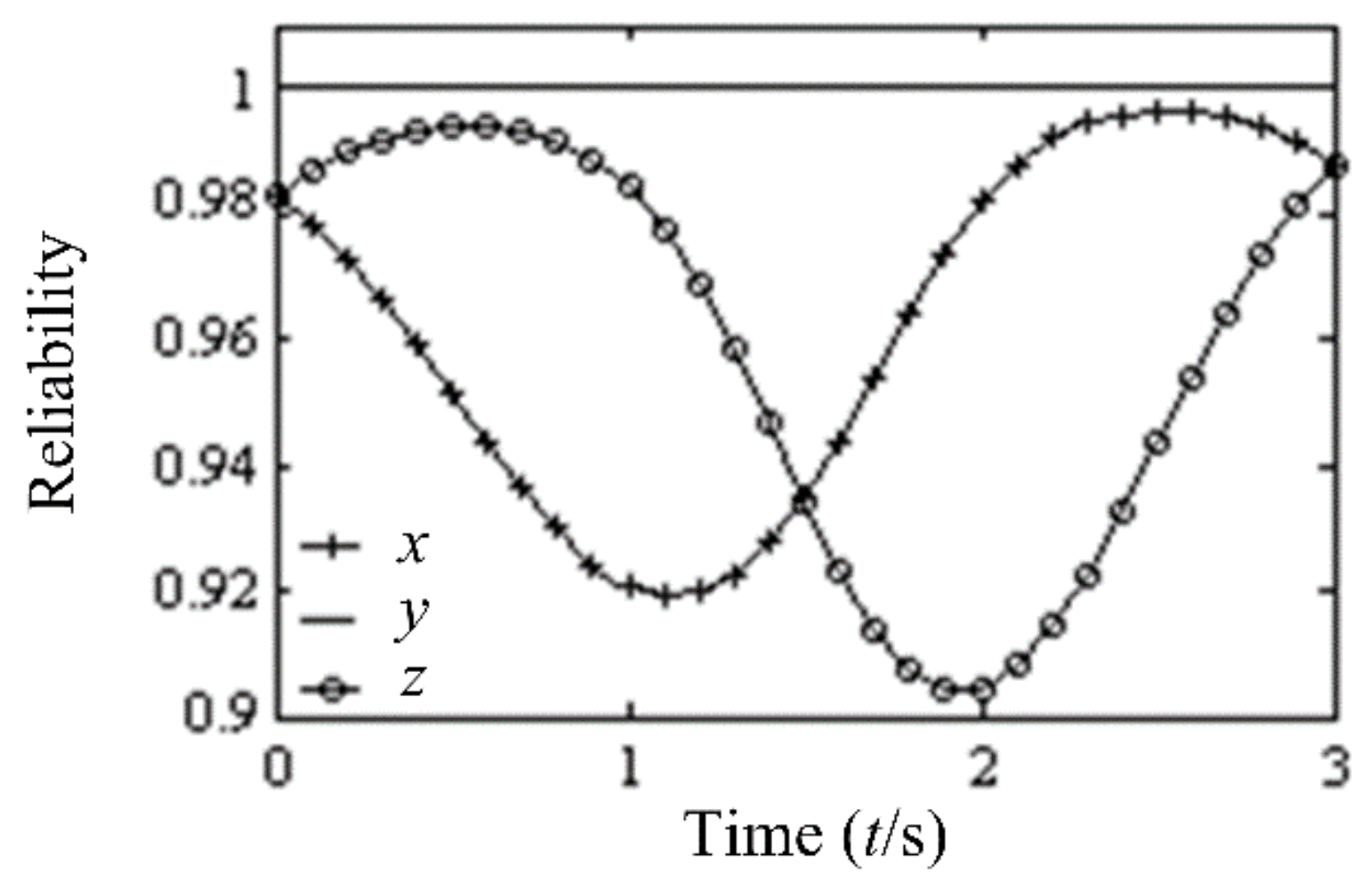
Figure 4 shows the change of the rotation angles of the three driving arms during the movement. When ${\epsilon }_1=-0.1$ and ${\epsilon }_2=0.1$, the results of the kinematic reliability in the x, y and z directions are as shown in Figure 5. The kinematic reliability of the mechanism in the y-direction is observed to be larger than that in the x and z directions corresponding to the given coordinate system and motion trajectory.

For the 12 random variables in Table 2, each random variable takes three level values, and 193 samples are obtained based on the same central point applying Box-Behnken sampling as shown in Appendix B (the same central point data are calculated as one). Meanwhile, according to each group of samples, the 193 corresponding output position errors of the mechanism at t = 0.5 s are calculated using a virtual prototype simulation and are listed in the last column of Appendix B.

According to the data in Appendix B and Equations (4) and (5), the response surface function Y of the output position error of the improved Delta parallel mechanism in the combined direction is obtained. Assuming that the maximum allowable limit of the mechanism is U = 1 mm, the limit state function g(x) is derived according to Equation (26).

$$g(x)=U-Y.$$

(38)

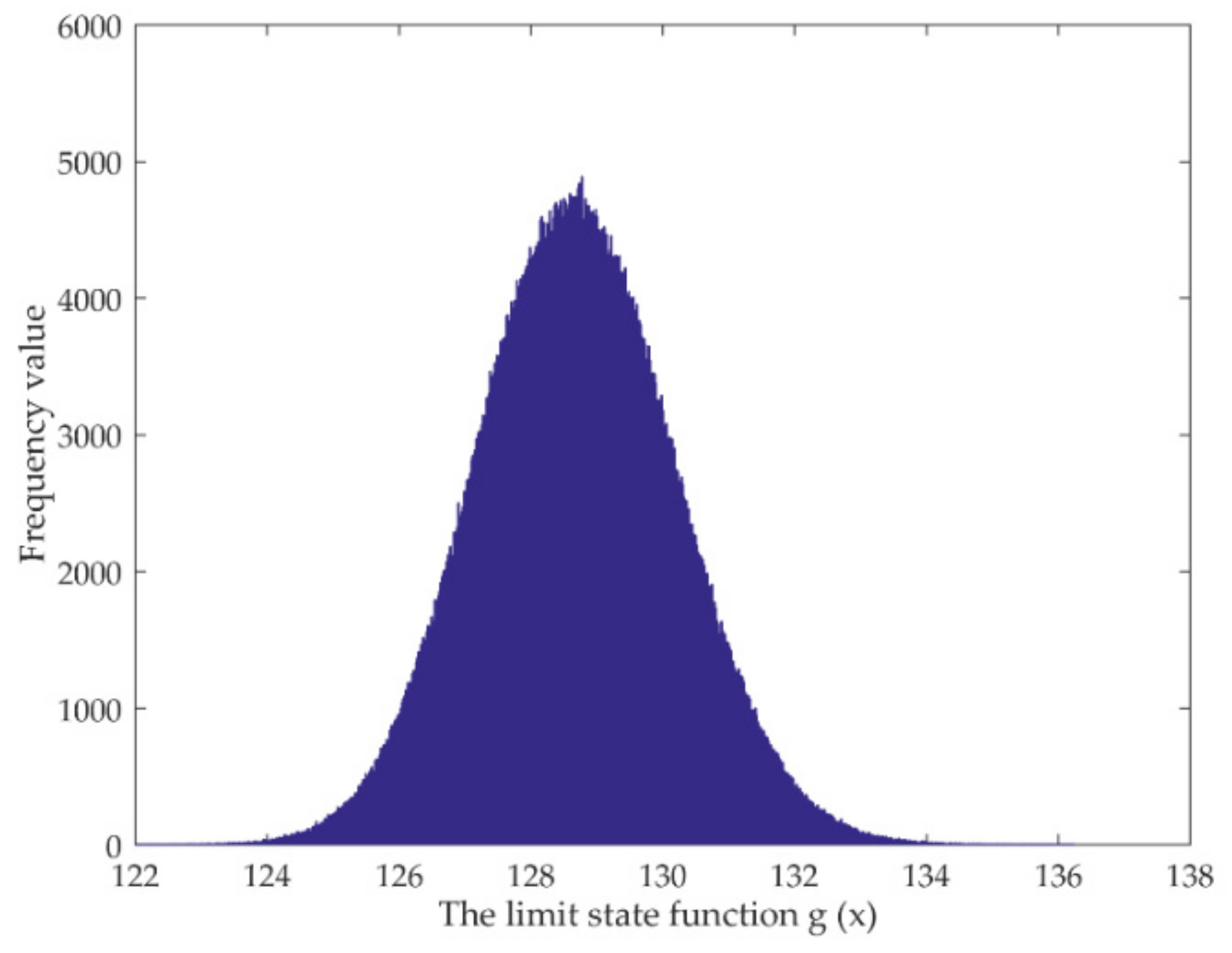
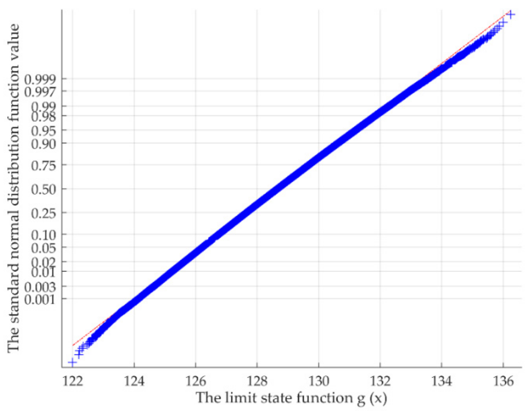
The limit state function g(x) is shown in Appendix Equation (A1). As shown in Figure 6, the frequency histogram of g(x) is obtained using the Monte Carlo method based on Equation (38). The g(x) distribution diagram is shown in Figure 7. The distribution is noted as linear indicating that g(x) has a normal distribution.

In addition, the data ${\mu }_g$ and ${ \sigma }_g$ are obtained through the Monte Carlo method based on Equation (38).

$${\mu }_g=128.6927{ \sigma }_g=40.0166$$

Then we can calculate the reliability index β and reliability R from Equations (33) and (34).

$$\beta =3.216, R=0.9994$$

From Equations (27), (28) and (31), the mean ${\mu }_g$ of the limit state function is obtained, with its expression shown in Appendix Equation (A2). From Equations (29), (30) and (32), the variance Dg is obtained, and the function expression is shown in Appendix Equation (A3).

According to Appendix Equation (A2) and Appendix Equation (A3), the values ${\mu }_g=128.0974$ and the ${ \sigma }_g=39.8660$ are calculated, which are nearly equal to the data calculated by the Monte Carlo method. Based on the Equations (34)–(37), the calculation results of reliability sensitivity are determined:

$$\begin{array}{c}\frac{\partial R}{\partial {\mu }^T}=(\frac{\partial R}{\partial {\mu }_1} \frac{\partial R}{\partial {\mu }_2} \frac{\partial R}{\partial {\mu }_3} \frac{\partial R}{\partial {\mu }_4} \frac{\partial R}{\partial {\mu }_5} \frac{\partial R}{\partial {\mu }_6} \frac{\partial R}{\partial {\mu }_7} \frac{\partial R}{\partial {\mu }_8} \frac{\partial R}{\partial {\mu }_9} \frac{\partial R}{\partial {\mu }_{10}} \frac{\partial R}{\partial {\mu }_{11}} \frac{\partial R}{\partial {\mu }_{12}} )\\ =(0.4114 -0.1889 -1.4998 0.7636 1.6337-0.6363 0.0015 0.1467 \\ -0.1288 -0.0492 0.01084 0.0796)\\ \frac{\partial R}{\partial D^T}=(\frac{\partial R}{\partial D_1} \frac{\partial R}{\partial D_2} \frac{\partial R}{\partial D_3} \frac{\partial R}{\partial D_4} \frac{\partial R}{\partial D_5} \frac{\partial R}{\partial D_6} \frac{\partial R}{\partial D_7} \frac{\partial R}{\partial D_8} \frac{\partial R}{\partial D_9} \frac{\partial R}{\partial D_{10}} \frac{\partial R}{\partial D_{11}} \frac{\partial R}{\partial D_{12}} )\\ =(-6.0553 -6.9927 -4.5702 -58.7828 -107.8470 -21.2619 -12.0916 \\ -2.3411 -24.7880 -0.0350 -0.01708 -0.04111)\end{array}$$

It can be obtained from the sensitivity matrix $\partial R/\partial {\mu }^T$ of kinematic reliability to the mean of the random parameter vector:

1.

Increasing the means of $\Delta r_{22}, \Delta r_{32}, \Delta a_3, \Delta {\phi }_3$ and $\Delta {\theta }_{11}$ will decrease the kinematic reliability of the mechanism, while the increase of the mean of the other errors will increase the kinematic reliability. The reliability of the improved Delta parallel mechanism with respect to the mean of the input errors is more sensitive to the changes in μ_Δa2, μ_Δr32, and μ_Δa1 than to the changes in μ_Δa3, with the mean sensitivities of the other errors being smaller. The mean sensitivity of the length error of the second driving arm $\left|\partial R/\partial {\mu }_{\Delta a2}{}_{ }\right|=1.6337$ is the largest, meaning the reliability could be improved to some extent by controlling the mean of Δa₂.

2.

The increase of the mean of the input errors does not wholly decrease the kinematic reliability of the mechanism, which indicates that the output position errors of the end-effector of the improved Delta parallel mechanism are caused by the coupling errors of each branch, and even the influences of the same kind of errors on kinematic reliability are also different because of the arrangements of the three branches.

It can be obtained from the variance sensitivity matrix $\partial R/\partial D^T$ of kinematic reliability to the variances of the random parameter vector:

1.

The increase in the variances of all the random parameters will decrease the kinematic reliability of the parallel mechanism. Therefore, in order to increase kinematic reliability of the improved Delta parallel mechanism, some effective measures could be taken to minimize the variances of the input errors of all the design variables at a reasonable cost controlled during processing and manufacturing.

2.

We can also learn that the variance reliability of kinematic accuracy of the improved Delta parallel mechanism is more sensitive to Δa₂, Δa₁, Δφ₃ and Δa₃ and followed by Δφ₁, Δr₂₂, Δr₁₂, Δr₃₂ and Δφ₂. The variance sensitivity of the length errors of the second driving arm $\left|\partial R/\partial D_{\Delta a2}{}_{ }\right|=107.847$ is the largest, and the average of variance sensitivity of Δa_i (i = 1, 2, 3) is equal to 62.6326 which is much larger than any other variance sensitivity. The increase in variances of driving arms have the most serious influence on the kinematic reliability. Therefore, the discreteness of length errors of the driving arms should be strictly controlled during machining and assembling to obtain desired kinematic reliability of the improved Delta parallel mechanism.

8. Conclusions

Kinematic reliability is an important index to evaluate repetitive positioning accuracy of mechanisms. Considering the randomness of input errors, kinematic reliability essentially reflects the performance of the mechanisms. This paper defines an index to evaluate the kinematic reliability of the improved Delta parallel mechanism and gives the corresponding calculation procedure. This provides a theoretical basis on kinematic reliability estimation of other parallel mechanisms.

The response surface method is used to calculate the kinematic reliability of the improved Delta parallel mechanism in the combined direction, R = 0.9994. Reliability sensitivity analysis indicates that:

1.

The kinematic reliability of the improved Delta parallel mechanism has the strongest sensitivity to the mean of $\Delta a_2$, followed by $\Delta r_{32}$,$\Delta a_1$ and $\Delta a_3$; while the mean sensitivities of other errors are comparatively small.

2.

The mean increase in each input error component does not wholly decrease the reliability of the mechanism, which indicates that the output positioning errors of the end-effector of the parallel mechanisms are caused by the coupling errors of each parallel branch. The increase in the variance of all the random variables reduces the kinematic reliability.

3.

Among all the input errors, the variance sensitivity to the length errors of the driving arms are the largest, which indicates that the increase in variance mostly decreases kinematic reliability of the improved Delta mechanism.

References

- Stewart, D. A platform with six degrees of freedom. Proceeding Inst. Mech. Eng. 1965, 180, 371–386. [Google Scholar] [CrossRef]
- Hunt, K.H. Structural kinematics of In-Parallel-Actuated Robot-Arms. ASME J. Transm. Autom. Des. 1983, 105, 705–712. [Google Scholar] [CrossRef]
- Clavel, R. Delta, a fast robot with parallel geometry. In Proceedings of the 18th International Symposium on Industrial Robots, Lausanne, Switzerland, 26–28 April 1988; pp. 91–100. [Google Scholar]
- Clavel, R. Device for the Movement and Positioning of an Element in Space. WO Patent No. WO8703528A1, 18 June 1987. [Google Scholar]
- Tsai, L.W. Multi-Degree-of-Freedom Mechanism for Machine Tools and the like. U. S Patent No. 5656905, 12 August 1997. [Google Scholar]
- Tsai, L.W.; Walsh, G.C.; Stamper, R.E. Kinematics of novel three DOF translational platforms. In Proceedings of the IEEE International Conference on Robotics and Automation, Minneapolis, MN, USA, 22–28 April 1996; pp. 3446–3451. [Google Scholar]
- Stamper, R.E.; Tsai, L.W.; Walsh, G.C. Optimization of a three DOF translational platform for well-conditioned workspace. In Proceedings of the 1997 IEEE International Conference on Robotics and Automation, Albuquerque, NM, USA, 25 April 1997; pp. 3250–3255. [Google Scholar]
- Gallardo-Alvarado, J.; Balmaceda-Santamaría, A.L.; Castillo-Castaneda, E. An application of screw theory to the kinematic analysis of a Delta-type robot. J. Mech. Sci. Technol. 2014, 28, 3785–3792. [Google Scholar] [CrossRef]
- Brinker, J.; Corves, B.; Takeda, Y. Kinematic performance evaluation of high-speed Delta parallel robots based on motion/force transmission indices. Mech. Mach. Theory 2018, 125, 111–125. [Google Scholar] [CrossRef]
- Lu, X.; Zhao, Y.; Liu, M. Self-learning interval type-2 fuzzy neural network controllers for trajectory control of a Delta parallel robot. Neurocomputing 2018, 283, 107–119. [Google Scholar] [CrossRef]
- Xu, D.T.; Sun, Z.L. Continuous Stiffness Mapping of Modified Delta Parallel Mechanism. J. Northeast. Univ. (Nat. Sci.) 2012, 33, 1465–1469. (In Chinese) [Google Scholar]
- Orsino, R.M.M.; Coelho, T.A.H.; Pesce, C.P. Analytical mechanics approaches in the dynamic modelling of Delta mechanism. Robotica 2015, 33, 953–973. [Google Scholar] [CrossRef]
- Kuo, Y.L. Mathematical modeling and analysis of the Delta robot with flexible links. Comput. Math. Appl. 2016, 71, 1973–1989. [Google Scholar] [CrossRef]
- Silva, V.G.; Tavakoli, M.; Marques, L. Optimization of a Three Degrees of Freedom DELTA Manipulator for Well-Conditioned Workspace with a Floating Point Genetic Algorithm. Int. J. Nat. Comput. Res. 2014, 4, 1–14. [Google Scholar] [CrossRef] [Green Version]
- Bounab, B. Multi-objective optimal design based kineto-elastostatic performance for the DELTA parallel mechanism. Robotica 2016, 34, 258–273. [Google Scholar] [CrossRef]
- Mazare, M.; Taghizadeh, M. Geometric Optimization of a Delta Type Parallel Robot Using Harmony Search Algorithm. Robotica 2019, 37, 1494–1512. [Google Scholar] [CrossRef]
- Lin, P.D.; Ehmann, K.F. Direct Volumetric Error Evaluation for Multi-Axis Machines. Int. J. Mach. Tool Manufact. 1993, 33, 675–694. [Google Scholar] [CrossRef]
- Wang, S.M.; Ehmann, K.F. Error model and accuracy analysis of a Six-DOF Stewart Platform. J. Manuf. Sci. Eng. 2002, 124, 286–296. [Google Scholar] [CrossRef]
- Tang, G.B.; Huang, T. Kinematic Calibration of Delta Robot. Chin. J. Mech. Eng. 2003, 39, 55–60. (In Chinese) [Google Scholar] [CrossRef]
- Zheng, H.; Tang, G.B. Error modeling and sensitivity analysis of Delta robot. J. Harbin Inst. Technol. 2009, 41, 252–255. (In Chinese) [Google Scholar]
- Wenchang, Z.; Jiangping, M.; Yi, L.; Xin, Z. Calibration of Delta parallel robot kinematic errors based on laser tracker. J. Tianjin Univ. (Sci. Technol.) 2013, 46, 257–262. (In Chinese) [Google Scholar]
- Ghazi, M.; Nazir, Q.; Butt, S.U.; Baqai, A.A. Accuracy analysis of 3-RSS Delta parallel manipulator. Procedia Manuf. 2018, 17, 174–182. [Google Scholar] [CrossRef]
- Andrioaia, D.; Stan, G.; Funaru, M.; Obreja, C. The Influence of Kinematic Joints Clearances on the Positioning Accuracy of 3DOF Delta Parallel Robots. Appl. Mech. Mater. 2013, 371, 406–410. [Google Scholar] [CrossRef]
- Andrioaia, D.; Stan, G.; Cristea, I. Influence of Dimensional Deviations on the Positioning Accuracy of Robots with Delta 3 DOF Parallel Structure. Appl. Mech. Mater. 2014, 657, 839–843. [Google Scholar] [CrossRef]
- Andrioaia, D.; Puiu, G.; Ghenadi, A. The Influence of the Errors Introduced by the Actuator on the Positioning Accuracy of the Robots with Parallel Delta 3 DOF. Appl. Mech. Mater. 2015, 809, 1225–1230. [Google Scholar] [CrossRef]
- Tian, C.; Zhang, D. Design and analysis of novel kinematically redundant reconfigurable generalized parallel manipulators. Mech. Mach. Theory 2021, 166, 104481. [Google Scholar] [CrossRef]
- Chen, Y.; Li, Y.; Yang, D.; Li, T. Research on Input Scheme Selection of a Novel Parallel Mechanism. J. Robot. 2021, 2021, 8784361. [Google Scholar] [CrossRef]
- Dastjerdi, A.H.; Sheikhi, M.M.; Masouleh, M.T. A complete analytical solution for the dimensional synthesis of 3-DOF delta parallel robot for a prescribed workspace. Mech. Mach. Theory 2020, 153, 103991. [Google Scholar] [CrossRef]
- Li, Y.; Shang, D.; Liu, Y. Kinematic modeling and error analysis of Delta robot considering parallelism error. Int. J. Adv. Robot. Syst. 2019, 16. [Google Scholar] [CrossRef]
- Shen, H.; Meng, Q.; Li, J.; Deng, J.; Wu, G. Kinematic sensitivity, parameter identification and calibration of a non-fully symmetric parallel Delta robot. Mech. Mach. Theory 2021, 161, 104311. [Google Scholar] [CrossRef]
- Box, G.E.; Behnken, D.W. Some New Three Level Designs for the Study of Quantitative Variables. Technometrics 1960, 2, 455–475. [Google Scholar] [CrossRef]
- Vining, G.G.; Kowalski, S.M.; Montgomery, D.C. Response Surface Designs within a Split-Plot Structure. J. Qual. Technol. 2005, 37, 115–129. [Google Scholar] [CrossRef]
- Soo, E.L.; Salleh, A.B.; Basri, M.; Rahman, R.A.; Kamaruddin, K. Response surface methodological study on lipase-catalyzed synthesis of amino acid surfactants. Process Biochem. 2004, 39, 1511–1518. [Google Scholar] [CrossRef]
- Lee, S.J. The Determination of the Probabilistic of Velocities and Acceleration in Kinematic Chain with Uncertainty. ASME J. Mech. Transm. Autom. Des. 1991, 113, 84–90. [Google Scholar] [CrossRef]
- Liu, W.X. Mechanical Reliability Design; Tsinghua University Press: Beijing, China, 2003. (In Chinese) [Google Scholar]
- Sun, Z.; Chen, L. Practical Design Theory and Method for Mechanical Reliability; Science Press: Beijing, China, 2003. (In Chinese) [Google Scholar]
- Jarmoluk, A.; Pietrasik, Z. Response surface methodology study on the effects of blood plasma, microbial transglutaminase and κ-carrageenan on pork batter gel properties. J. Food Eng. 2003, 60, 327–334. [Google Scholar] [CrossRef]
Figure 1.
Box-Behnke samples of three variables.
Figure 2.
Kinematic sketch of the improved Delta mechanism.
Figure 3.
Kinematic sketch of each branch.
Figure 4.
Change of the rotation angle of three driving arms.
Figure 5.
Calculation results of kinematic reliability.
Figure 6.
Frequency distribution histogram of g(x).
Figure 7.
Normal distribution test of g(x).