
Automated Vehicle’s Overtaking Maneuver with Yielding to Oncoming Vehicles in Urban Area Based on Model Predictive Control


Abstract
:1. Introduction
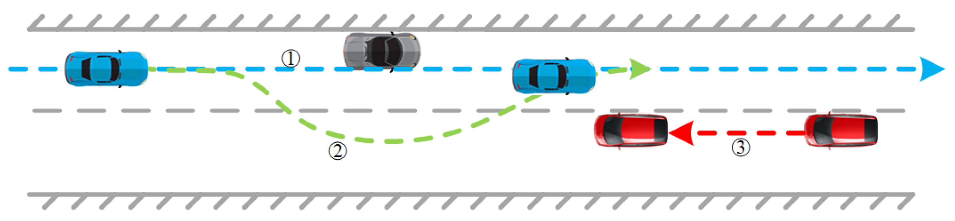
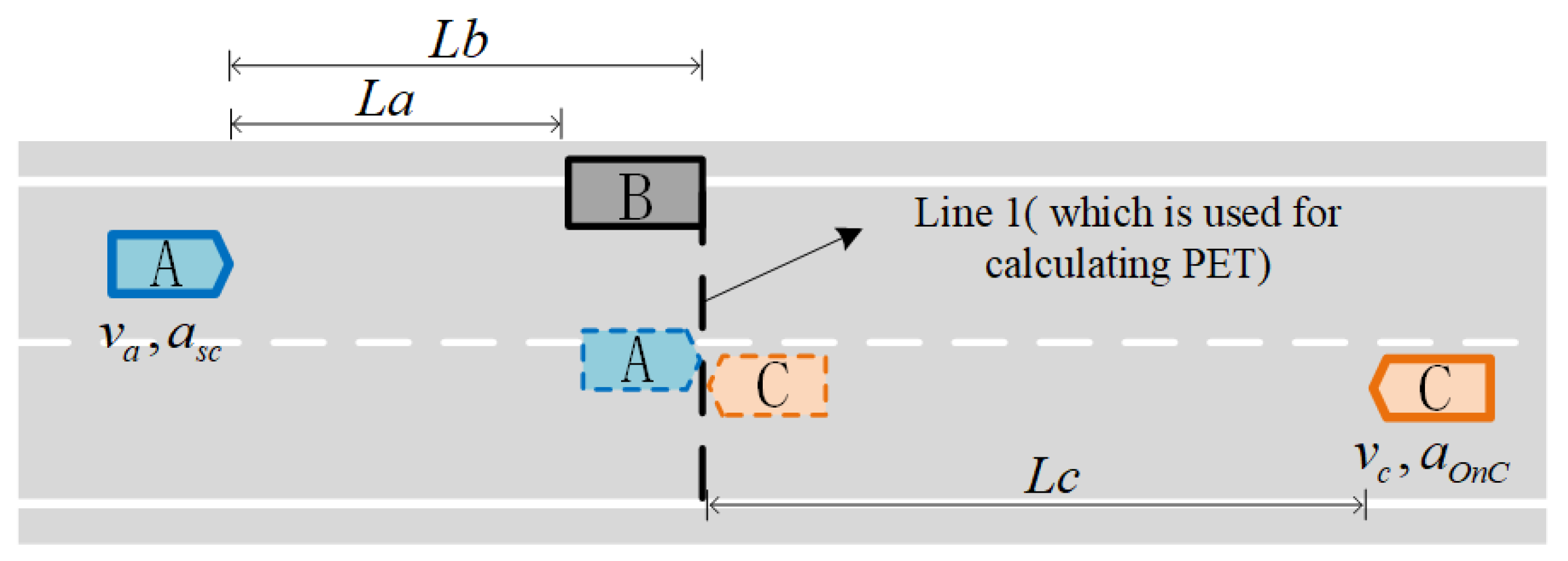
2. Scenario
- (1)
- La, Lb are global fixed parameters for the scenario, that means the initial relative position of the ego vehicle and the parked vehicle are not changed in any simulation;
- (2)
- Lc is treated as a local invariant, that means the initial relative position of the ego vehicle and the parked vehicle will only be changed as the initial condition of a simulation;
- (3)
- , ;
- (4)
- , .
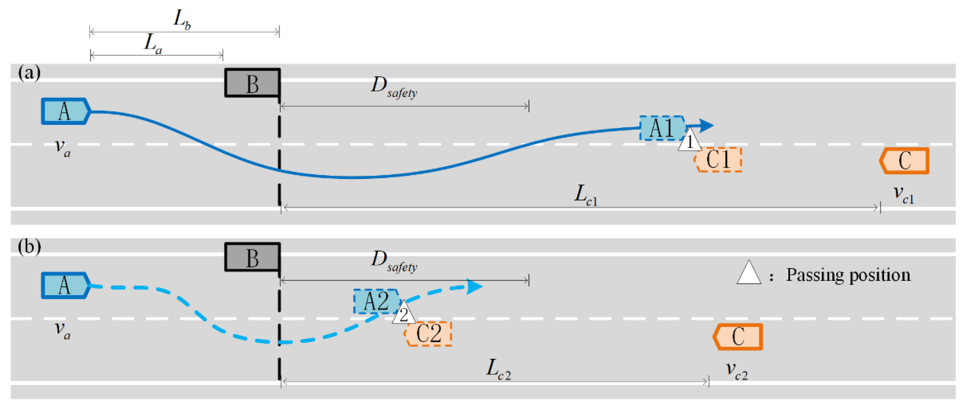
- (1)
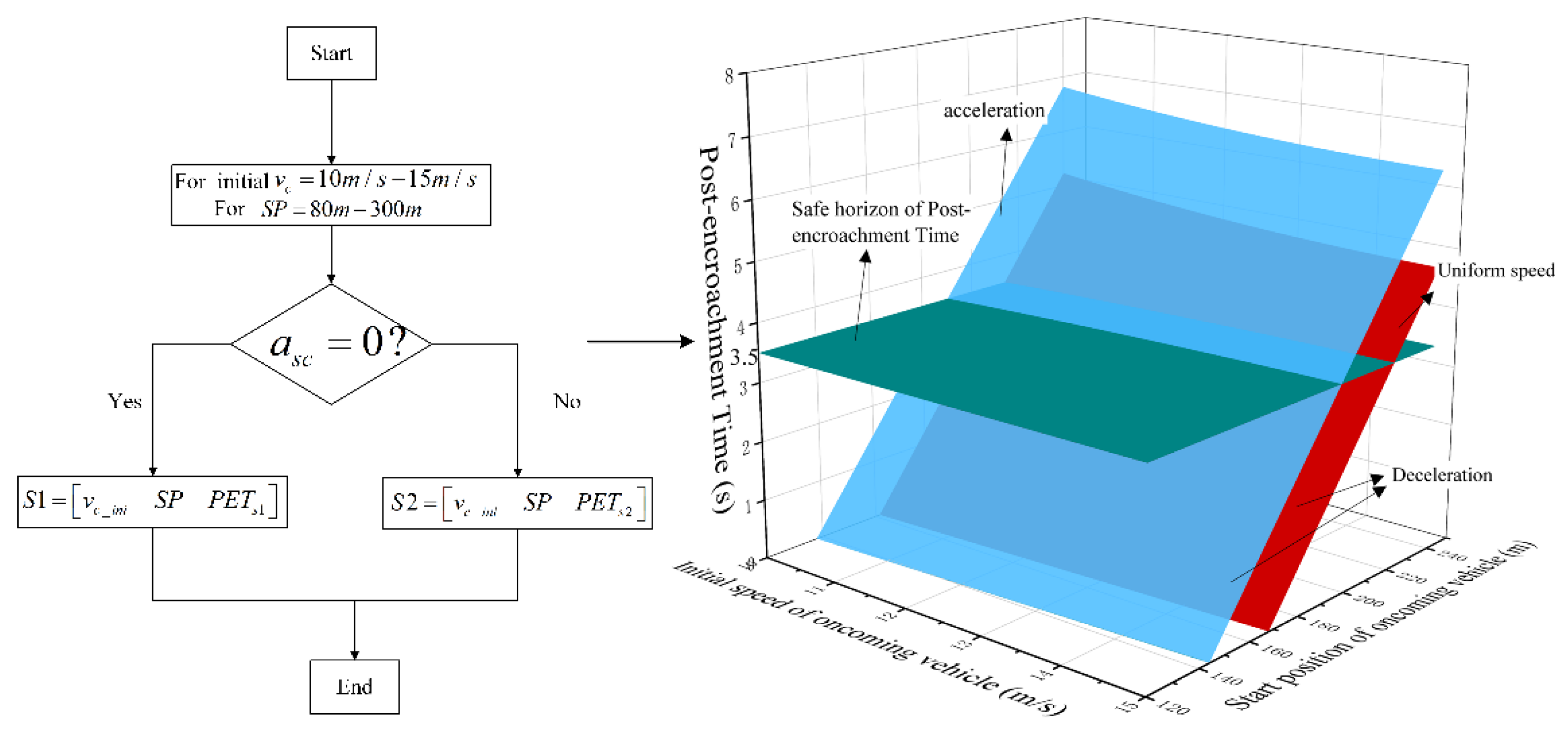
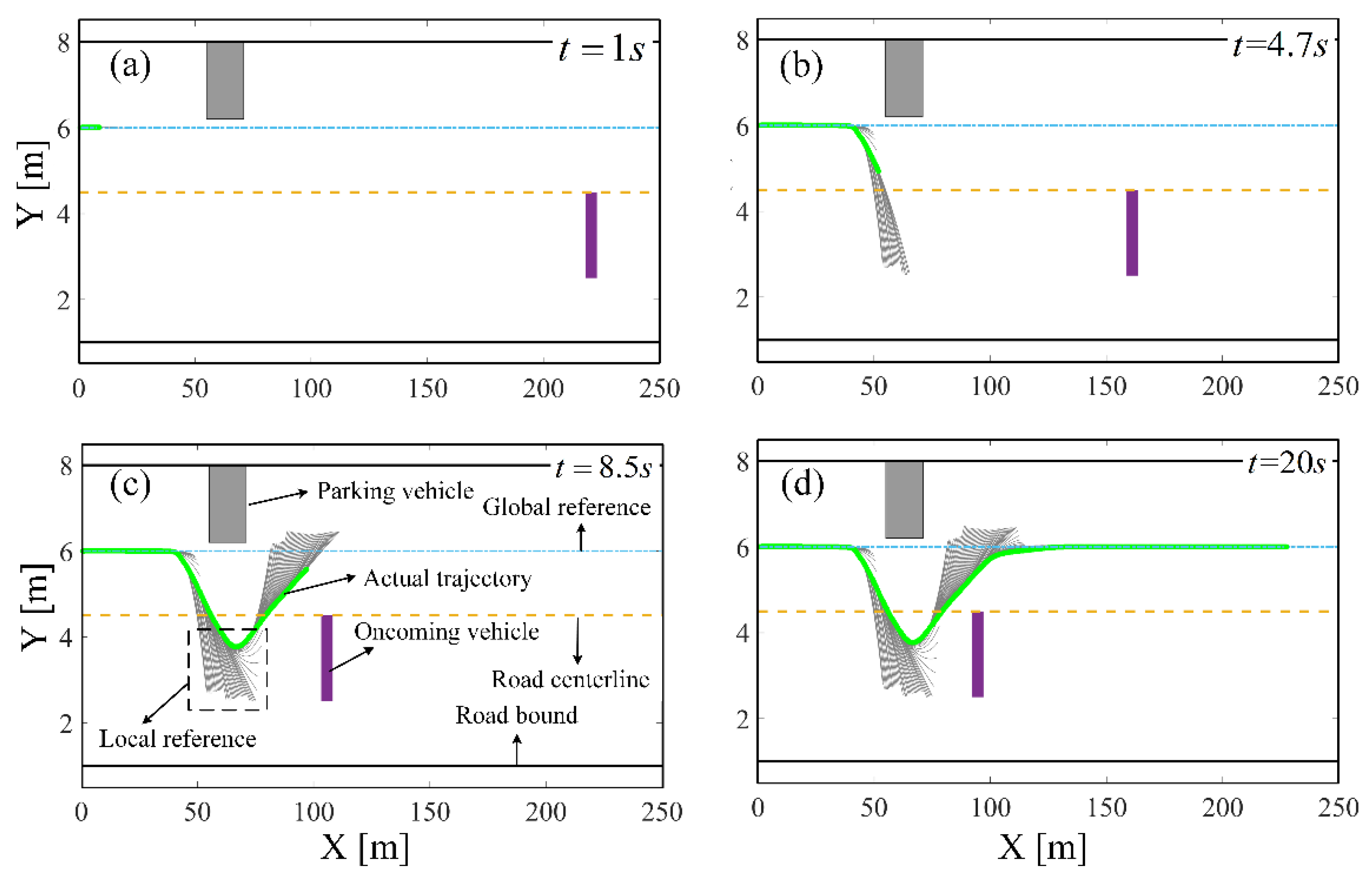
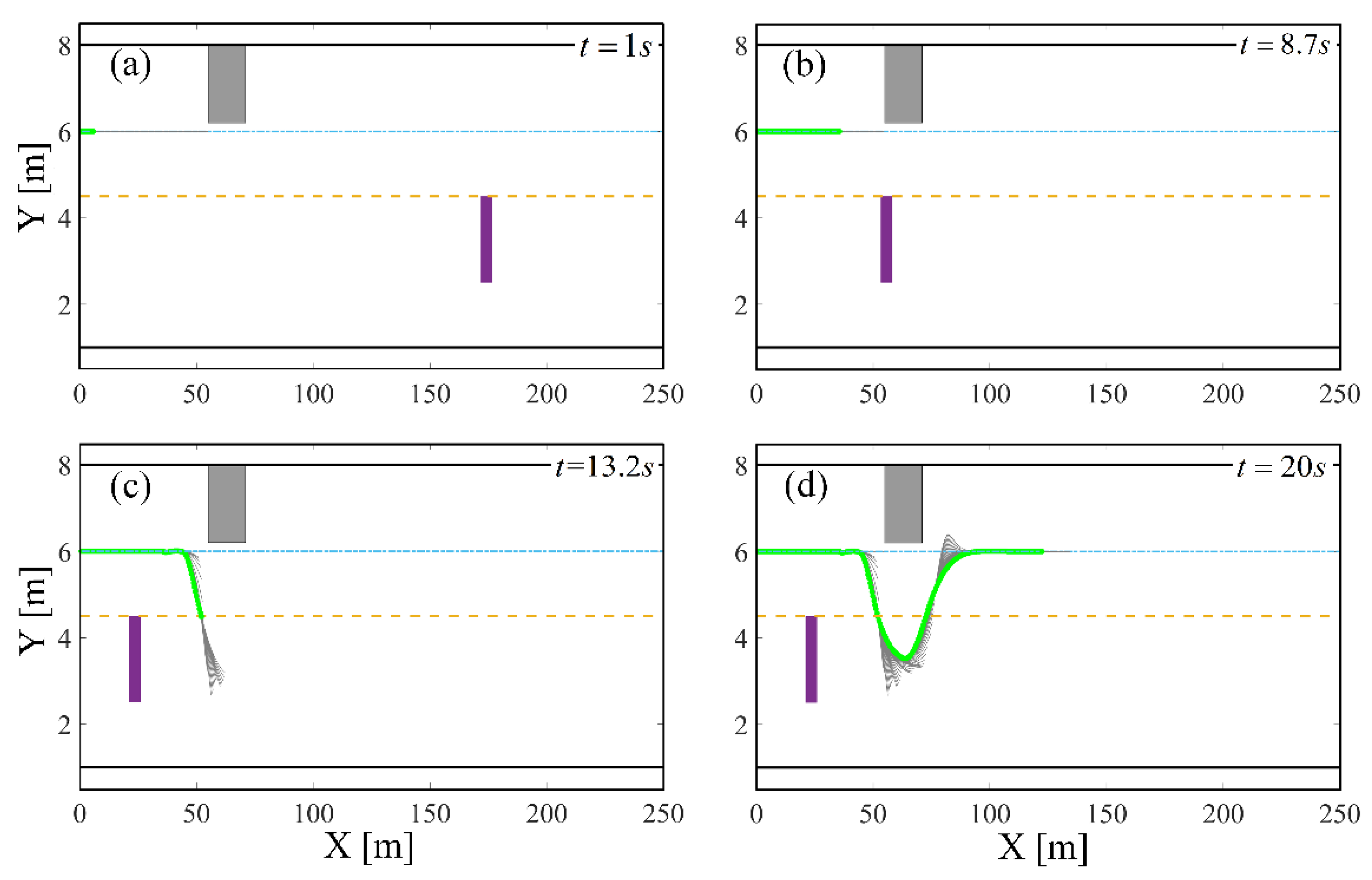
- If the passing position is far enough away from the parked vehicle, as shown in Figure 2a at passing position 1, the ego vehicle will choose to keep speed unchanged or accelerate according to the oncoming vehicle speed and position ;
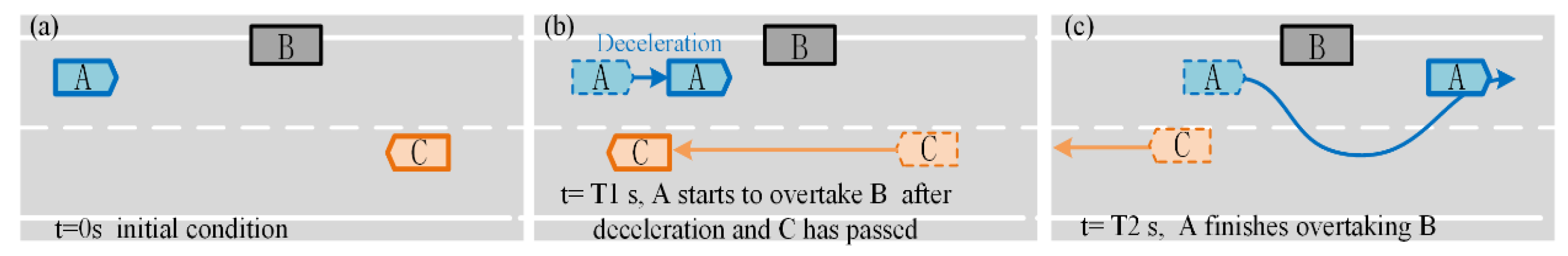
- (2)
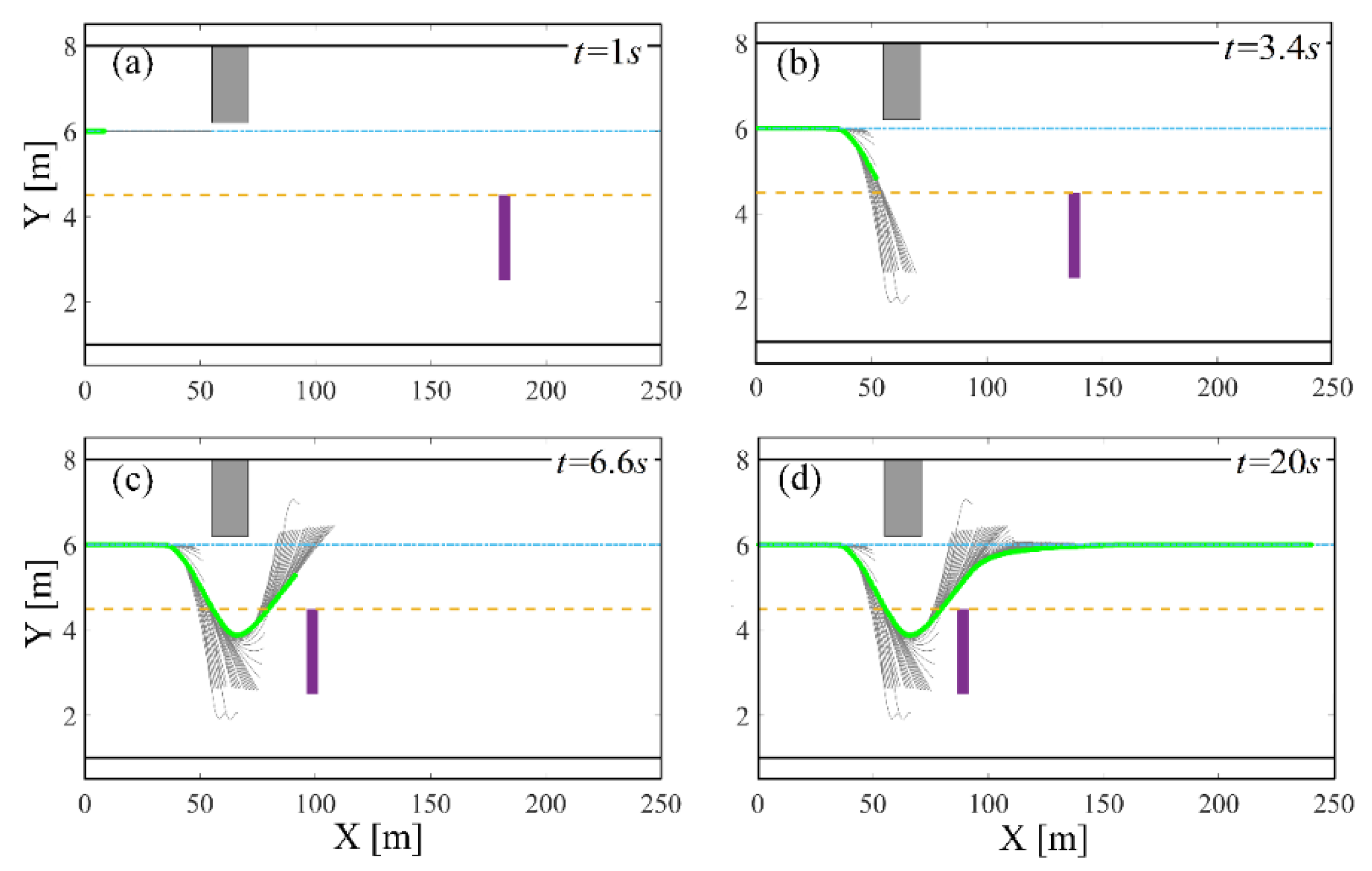
- Due to excessive speed or short initial distance of the oncoming vehicle, even if the ego vehicle accelerates to the maximum allowable speed, it cannot guarantee that their passing position is at a safe position, as shown in Figure 2b at passing position 2. The ego vehicle will decelerate until oncoming vehicle has already passed, shown as Figure 3, then it restarts and overtakes the parked vehicle.
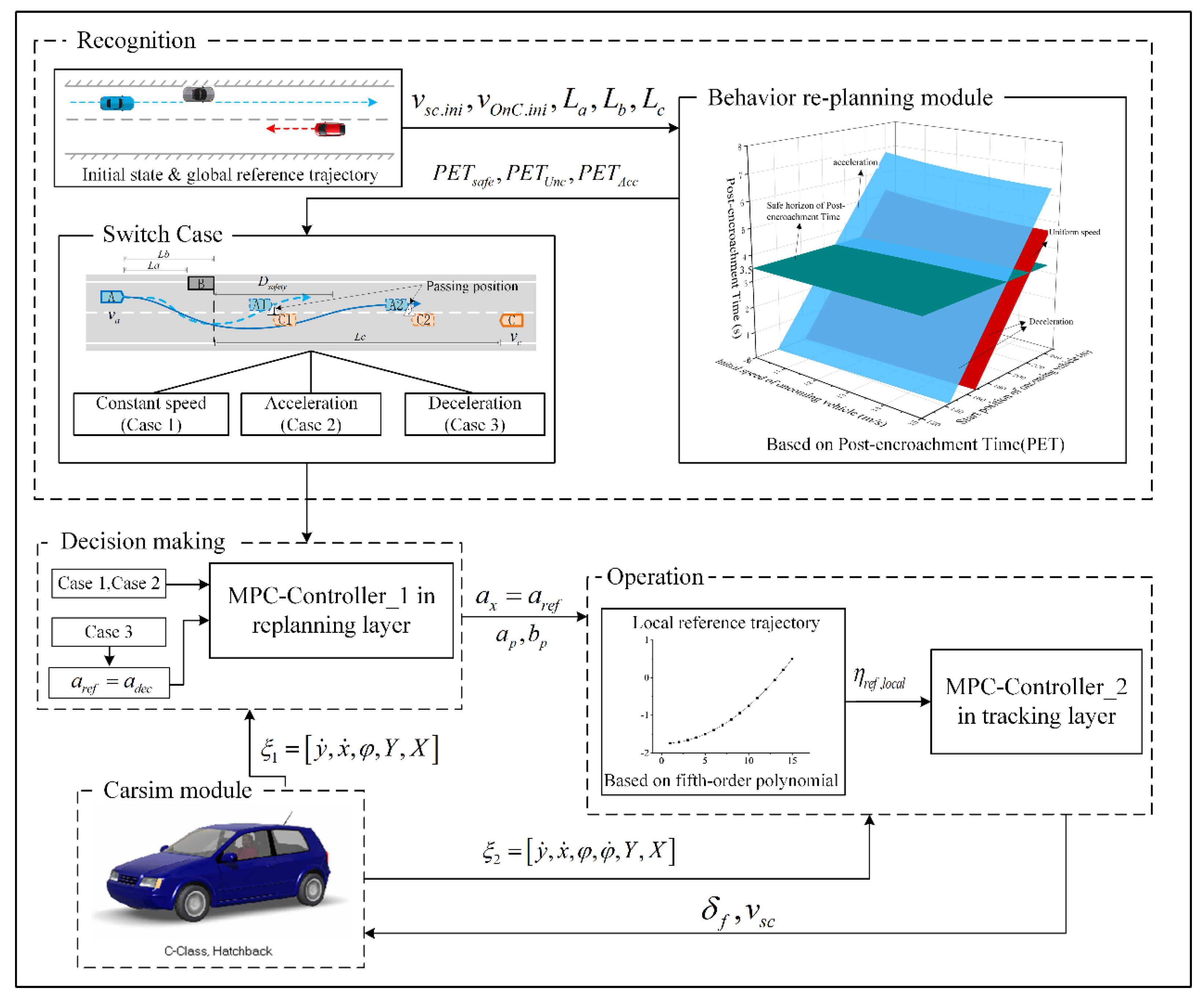
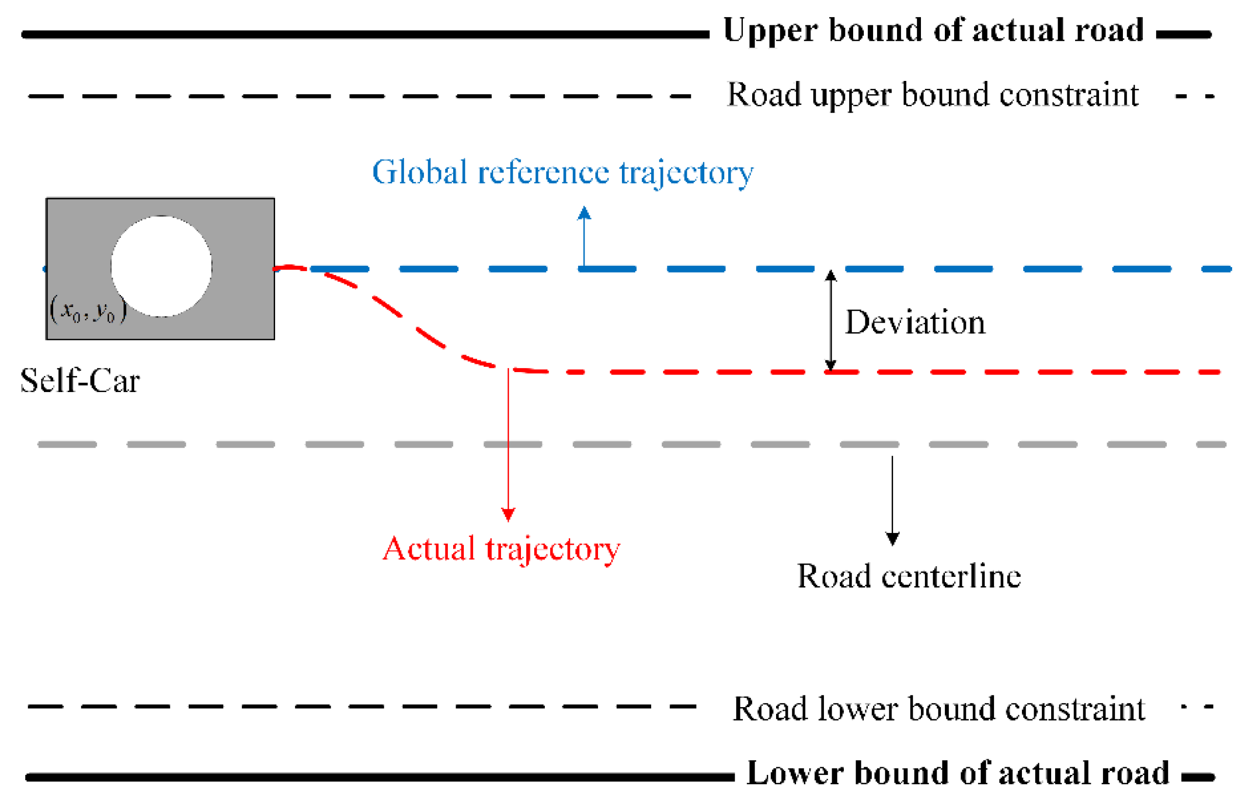
3. Collision Avoidance Strategy
3.1. Behavior Replanning Based on Post-Encroachment Time (PET)
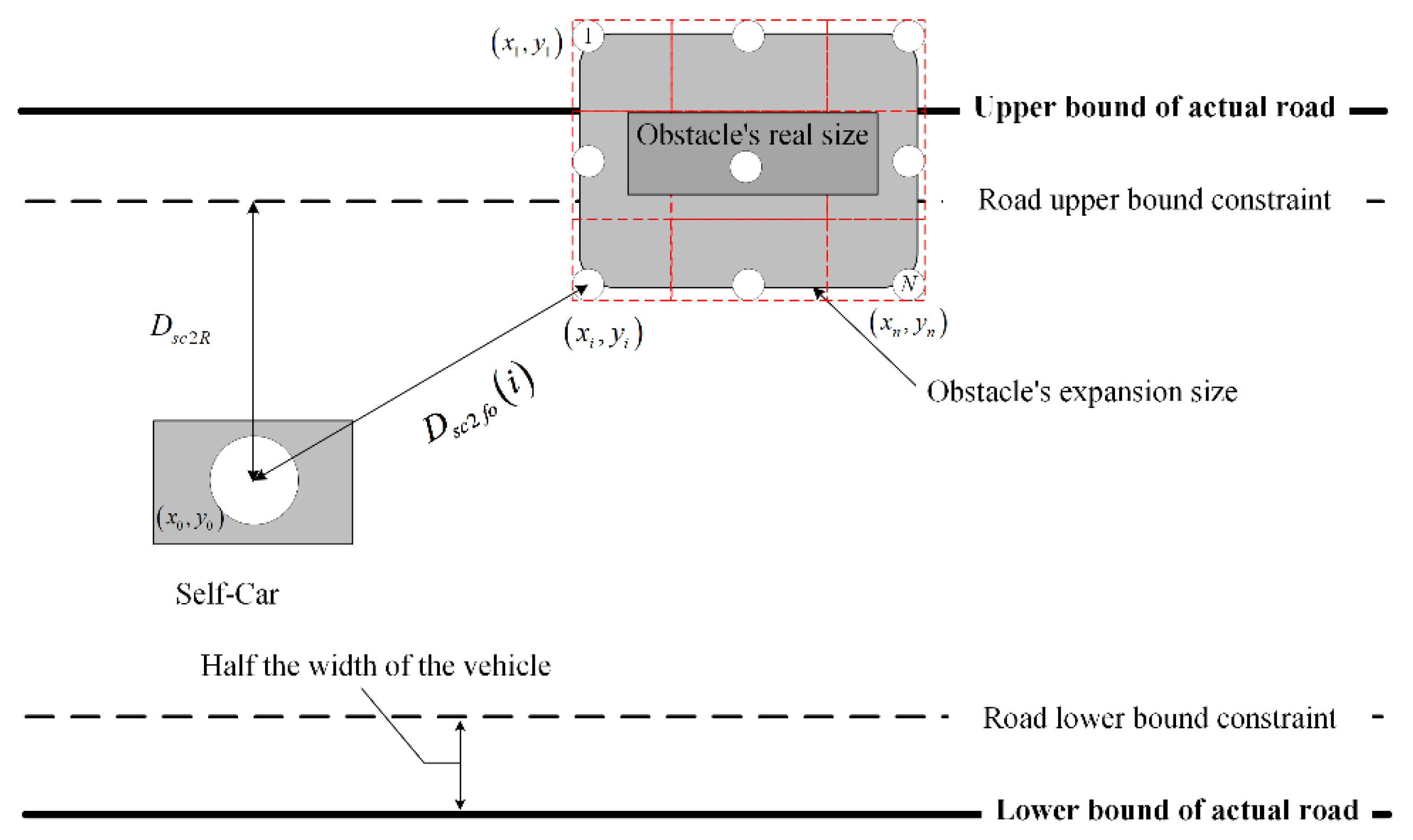
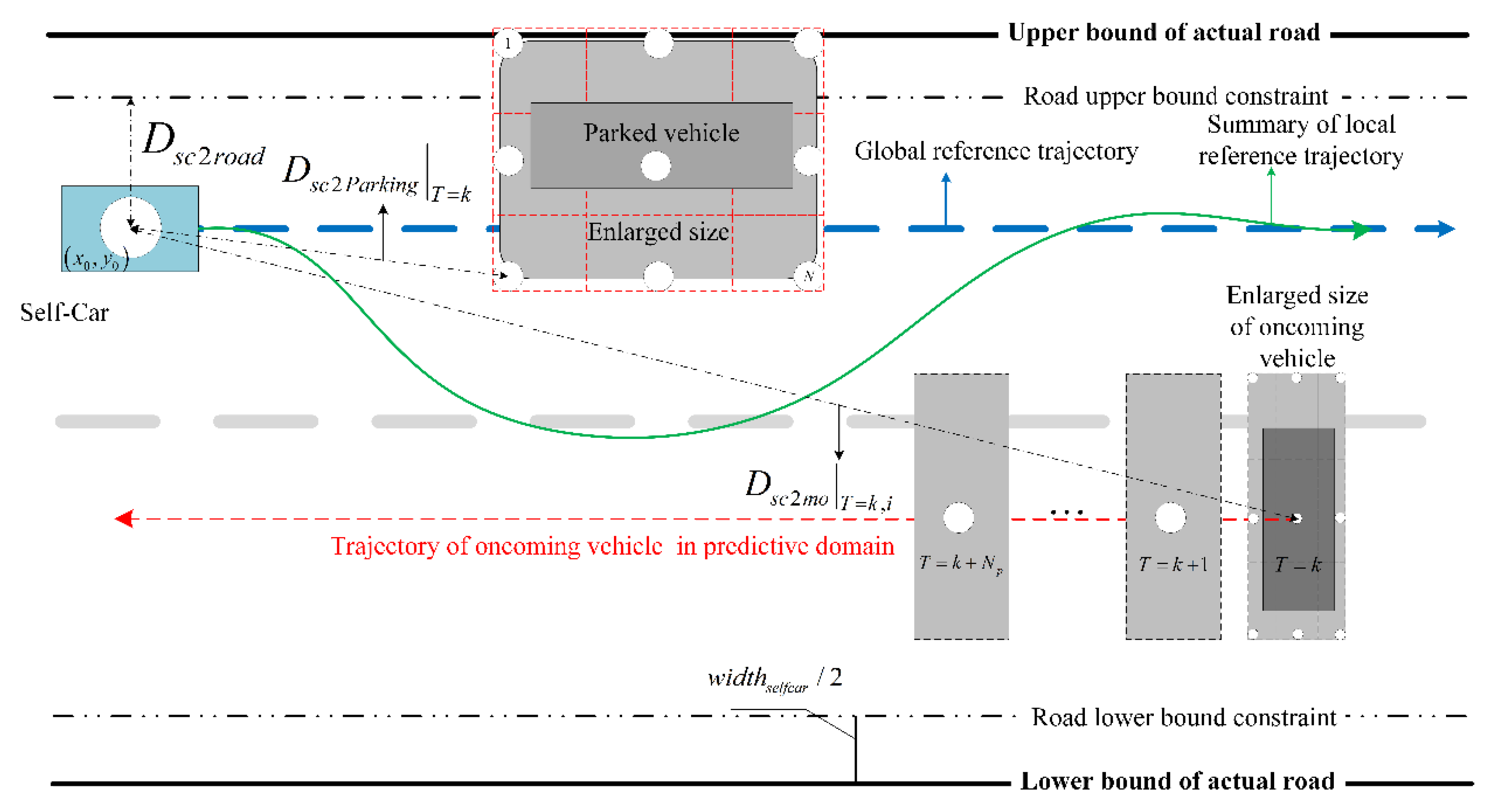
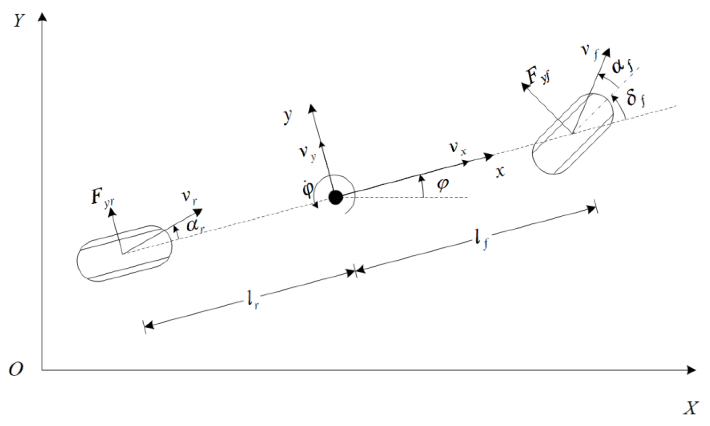
3.2. Two-Layer Model Predictive Control (MPC) Modeling
- (1)
- The actual boundary of the road should be preprocessed according to the width of the ego vehicle;
- (2)
- The parked vehicle is decomposed into several discrete small obstacles;
- (3)
- The cost of the function is adjusted by the vehicle speed and the distance deviation between the obstacle points and the vehicle.
3.2.1. Polynomial Fitting
3.2.2. Reference Trajectory Tracking Layer
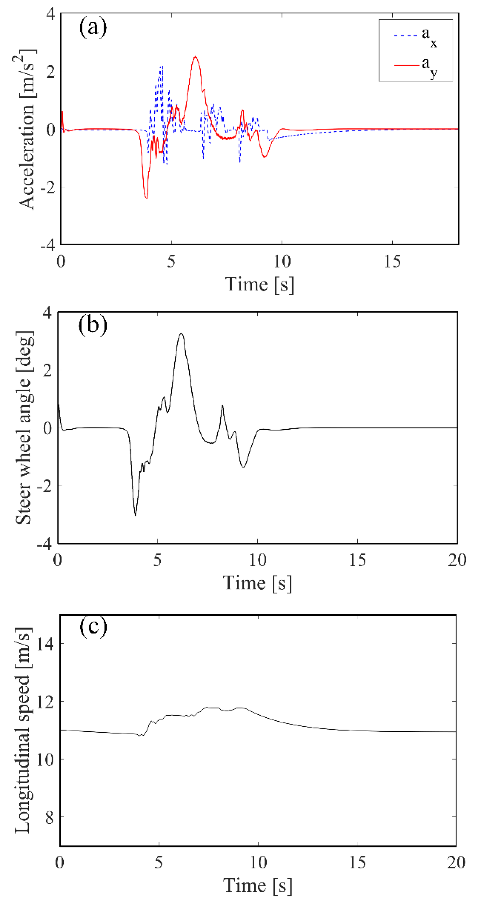
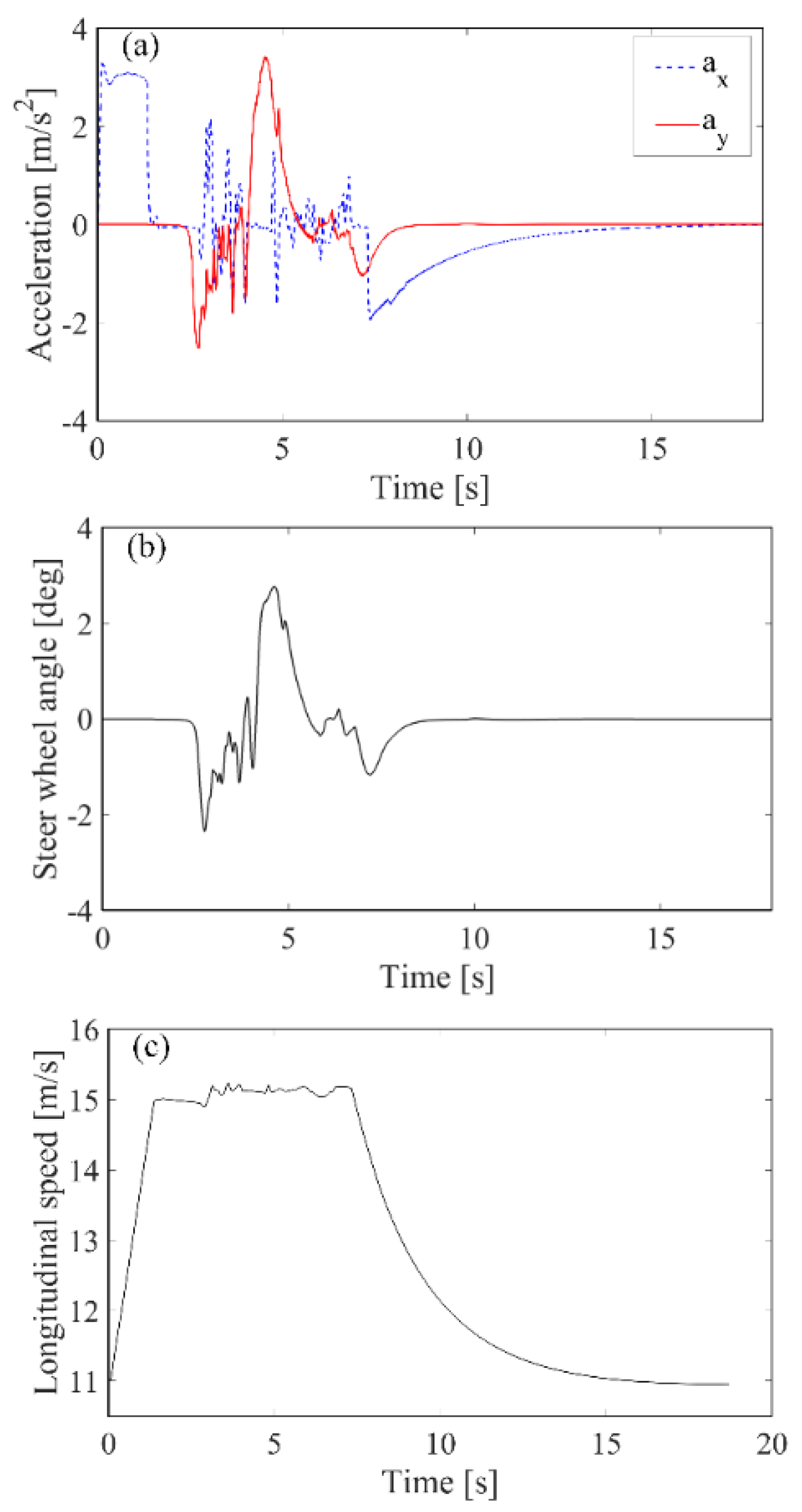
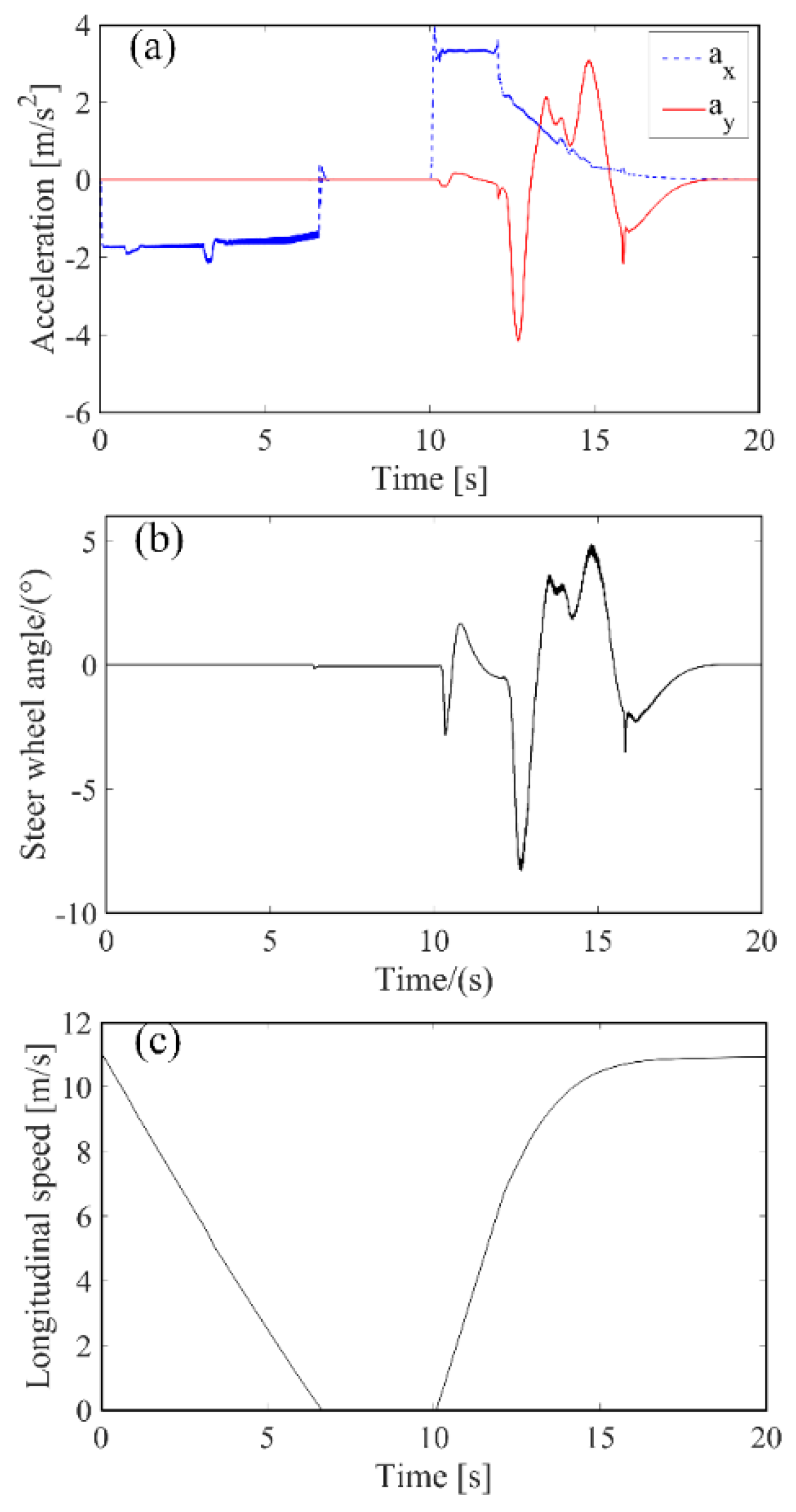
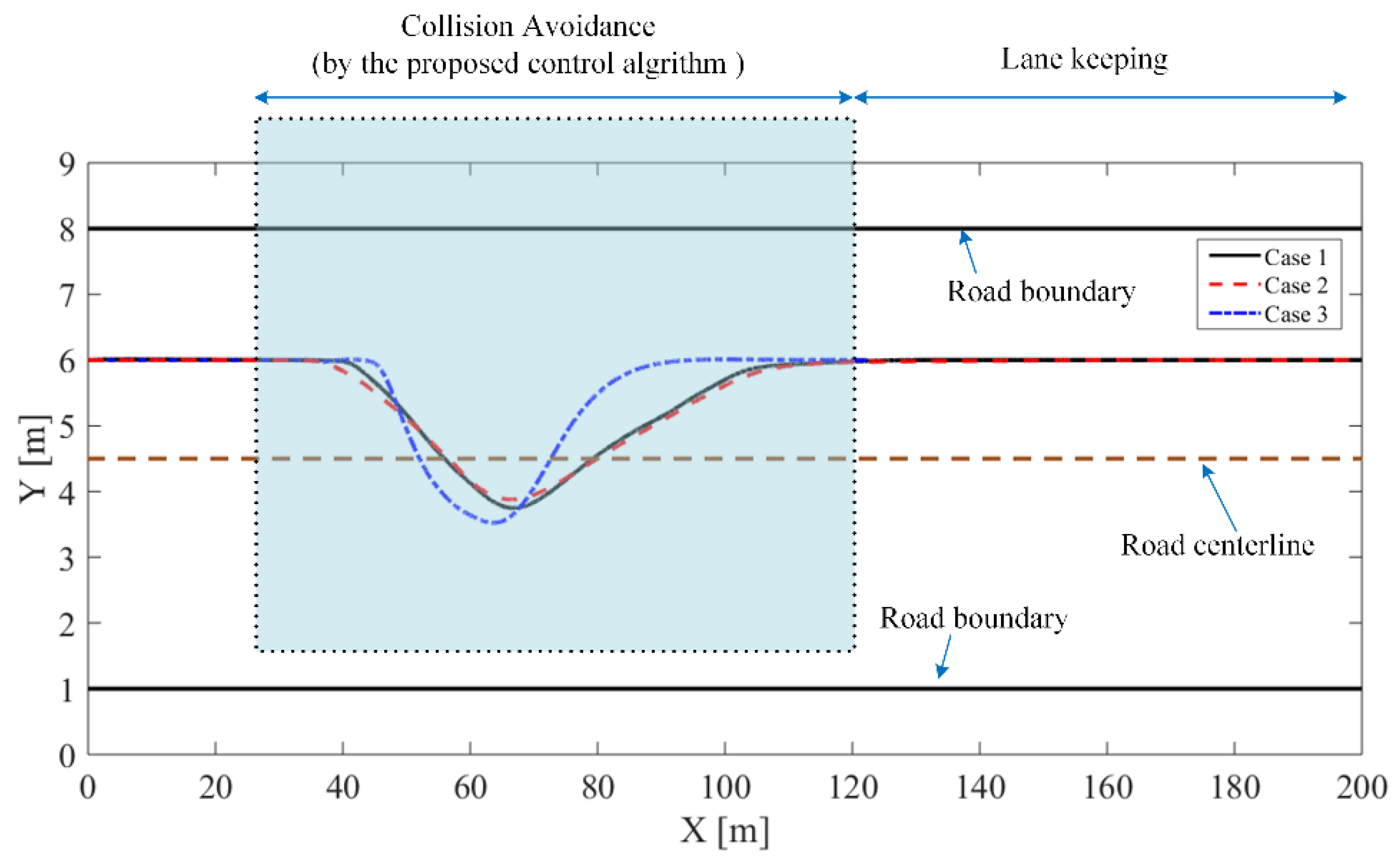
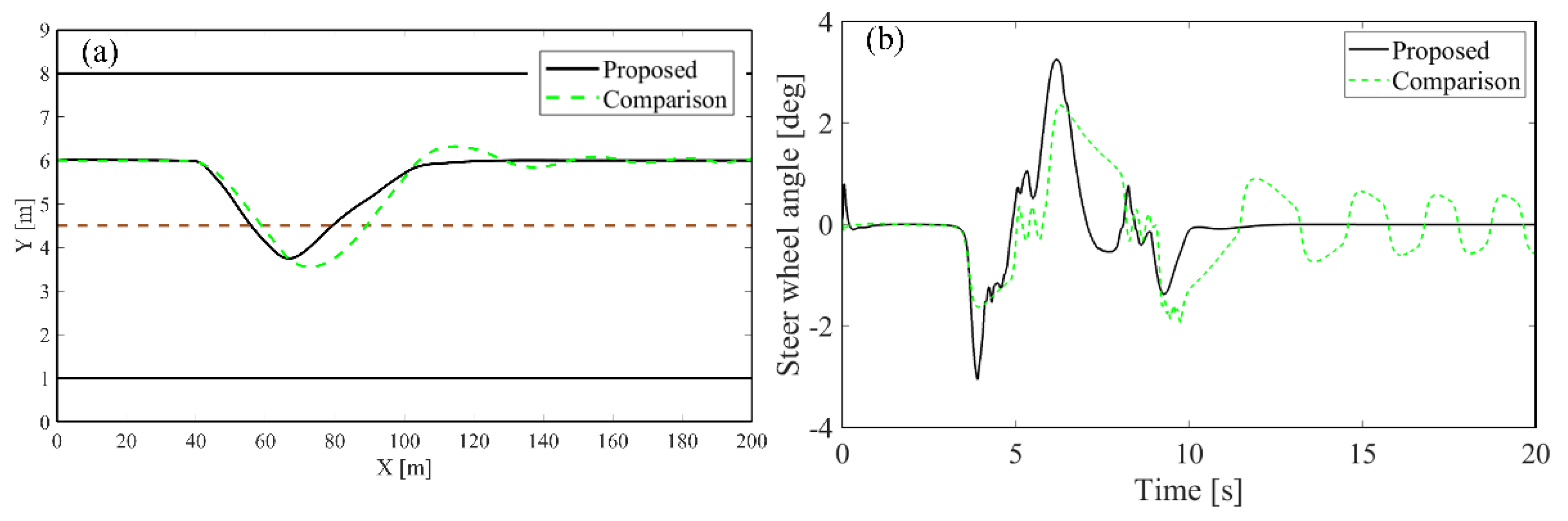
4. Simulation Results
5. Conclusions
Author Contributions
Funding
Institutional Review Board Statement
Informed Consent Statement
Data Availability Statement
Conflicts of Interest
References
- Fleming, W. Forty-Year Review of Automotive Electronics: A Unique Source of Historical Information on Automotive Electronics. IEEE Veh. Technol. Mag. 2015, 10, 89–90. [Google Scholar] [CrossRef]
- Shen, X.; Raksincharoensak, P. Pedestrian-aware statistical risk assessment. IEEE Trans. Intell. Transp. Syst. 2021. [Google Scholar] [CrossRef]
- Cheng, S.; Li, L.; Liu, C.Z.; Wu, X.; Yong, J.W. Robust lmi-based h-infinite controller integrating afs and dyc of autonomous vehicles with parametric uncertainties. IEEE Trans. Syst. Man Cybern. Syst. 2020, 99, 1–10. [Google Scholar] [CrossRef]
- Shen, X.; Zhang, Y.; Shen, T.; Khajorntraidet, C. Spark advance self-optimization with knock probability threshold for lean-burn operation mode of si engine. Energy 2017, 122, 1–10. [Google Scholar] [CrossRef]
- Fallon, I.; O’Neill, D. The world’s first automobile fatality. Accid. Anal. Prev. 2005, 37, 601–603. [Google Scholar] [CrossRef]
- He, H.; Paichadze, N.; Hyder, A.A.; Bishai, D. Economic development and road traffic fatalities in Russia: Analysis of federal regions 2004–2011. Inj. Epidemiol. 2015, 2, 1–16. [Google Scholar] [CrossRef] [Green Version]
- Hamlet, A.J.; Emami, P.; Crane, C.D. The cognitive driving framework: Joint inference for collision prediction and avoidance in autonomous vehicles. In Proceedings of the 15th International Conference on Control, Automation and Systems (ICCAS) IEEE, Edinburgh, UK, 16–19 July 2015. [Google Scholar]
- Vahidi, A.; Eskandarian, A. Research advances in intelligent collision avoidance and adaptive cruise control. Intell. Transp. Syst. IEEE Trans. 2003, 4, 143–153. [Google Scholar] [CrossRef] [Green Version]
- Li, X.; Seignez, E. Driver inattention monitoring system based on multimodal fusion with visual cues to improve driving safety. Trans. Inst. Meas. Control 2016, 40, 885–895. [Google Scholar] [CrossRef]
- Isermann, R.; Mannale, R.; Schmitt, K. Collision-avoidance systems proreta: Situation analysis and intervention control. Control Eng. Pract. 2012, 20, 1236–1246. [Google Scholar] [CrossRef]
- Shen, X.; Zhang, X.; Ouyang, T.; Li, Y.; Raksincharoensak, P. Cooperative comfortable-driving at signalized intersections for connected and automated vehicles. IEEE Robot. Autom. Lett. 2020, 5, 6247–6254. [Google Scholar] [CrossRef]
- Saito, Y.; Raksincharoensak, P. Risk predictive shared deceleration control: Its functionality and effectiveness of an early intervention support. In Proceedings of the IEEE Intelligent Vehicles Symposium (IV), Gotenburg, Sweden, 19–22 June 2016; pp. 49–54. [Google Scholar]
- Lefèvre, S.; Carvalho, A.; Borrelli, F. A learning-based framework for velocity control in autonomous driving. IEEE Trans. Autom. Sci. Eng. 2016, 13, 32–42. [Google Scholar] [CrossRef]
- Raksincharoensak, P.; Hasegawa, T.; Nagai, M. Motion planning and control of autonomous driving intelligence system based on risk potential optimization framework. Int. J. Automot. Eng. 2016, 7, 53–60. [Google Scholar] [CrossRef] [Green Version]
- Falcone, P.; Borrelli, F.; Asgari, J.; Tseng, H.E.; Hrovat, D. Predictive active steering control for autonomous vehicle systems. IEEE Trans. Control Syst. Technol. 2007, 15, 566–580. [Google Scholar] [CrossRef]
- Wang, T.-C.; Lin, T.-J. Unmanned vehicle obstacle detection and avoidance using danger zone approach. Trans. Can. Soc. Mech. Eng. 2013, 37, 529–538. [Google Scholar] [CrossRef]
- Gray, A.; Ali, M.; Gao, Y.; Hedrick, J.K.; Borrelli, F. Integrated threat assessment and control design for roadway departure avoidance. In Proceedings of the 15th International IEEE Conference on Intelligent Transportation Systems (ITSC), Anchorage, AK, USA, 16 September 2012; pp. 1714–1719. [Google Scholar]
- Cheng, S.; Li, L.; Liu, Y.; Li, W.; Guo, H. Virtual Fluid-Flow-Model-Based Lane-Keeping Integrated With Collision Avoidance Control System Design for Autonomous Vehicles. IEEE Trans. Intell. Transp. Syst. 2020, 99, 1–10. [Google Scholar] [CrossRef]
- Balachandran, A.; Brown, M.; Erlien, S.; Gerdes, J. Predictive Haptic Feedback for Obstacle Avoidance Based on Model Predictive Control. IEEE Trans. Autom. Sci. Eng. 2016, 13, 26–31. [Google Scholar] [CrossRef]
- Chi, K.-H.; Lee, M.-F.R. Obstacle avoidance in mobile robot using neural network. In Proceedings of the International Conference on Consumer Electronics, Communications and Networks (CECNet), XianNing, China, 16–18 April 2011; pp. 5082–5085. [Google Scholar]
- Duguleana, M.; Barbuceanu, F.G.; Teirelbar, A.; Mogan, G. Obstacle avoidance of redundant manipulators using neural networks based reinforcement learning. Robot. Comput. Integr. Manuf. 2012, 28, 132–146. [Google Scholar] [CrossRef]
- Huang, Y. Intelligent technique for robot path planning using artificial neural network and adaptive ant colony optimization. J. Converg. Inf. Technol. 2012, 7, 246–252. [Google Scholar]
- Chakravarthy, A.; Ghose, D. Generalization of the collision cone approach for motion safety in 3-d environments. Auton. Robot. 2012, 32, 243–266. [Google Scholar] [CrossRef]
- Balch, T.; Arkin, R.C. Behaviour-based formation control for multirobot teams. IEEE Trans. Robot. Autom. 1998, 14, 926–939. [Google Scholar] [CrossRef] [Green Version]
- Baker, J.E. Adaptive selection methods for genetic algorithms. In Proceedings of the International Conference on Genetic Algorithms and Their Applications, Hillsdale, NJ, USA, 24–26 July 1985; pp. 101–111. [Google Scholar]
- Yuan, H.; Sun, X.; Gordon, T. Unified decision-making and control for highway collision avoidance using active front steer and individual wheel torque control. Veh. Syst. Dyn. 2019, 57, 1188–1205. [Google Scholar] [CrossRef]
- Lefèvre, S.; Vasquez, D.; Laugier, C. A survey on motion prediction and risk assessment for intelligent vehicles. Robomech J. 2014, 1, 1–14. [Google Scholar] [CrossRef] [Green Version]
- Vogel, K. A comparison of headway and time to collision as safety indicators. Accid. Anal. Prev. 2003, 35, 427–433. [Google Scholar] [CrossRef]
- Falcone, P. Nonlinear Model Predictive Control for Autonomous Vehicles; University of Sannio: Benevento, Italy, 2007. [Google Scholar]
- Gong, J.W.; Jiang, Y.; Xu, W. Model Predictive Control for Self-Driving Vehicles; Beijing Institute of Technology Press: Beijing, China, 2014. [Google Scholar]
- Lattarulo, R.; He, D.; Perez, J. A Linear Model Predictive Planning Approach for Overtaking Manoeuvres under Possible Collision Circumstances. In Proceedings of the IEEE Intelligent Vehicles Symposium, Suzhou, China, 26–30 June 2018; pp. 1340–1345. [Google Scholar]


| A | ||
| Symbol | Value | Unit |
| 60 | (none) | |
| 2 | (none) | |
| (none) | ||
| (none) | ||
| 0.02 | s | |
| (none) | ||
| (none) | ||
| (none) | ||
| B | ||
| Symbol | Value | Unit |
| 30 | (none) | |
| 3 | (none) | |
| (none) | ||
| (none) | ||
| 1000 | (none) | |
| 0.01 | s | |
| A | ||
| Symbol | Range | Unit |
| Longitudinal speed | 10.8~11.8 | m/s |
| Steering wheel angle | −3.1~3.2 | °(degree) |
| Longitudinal acceleration | −1.2~2.2 | m/s2 |
| Lateral acceleration | −2.4~2.5 | m/s2 |
| B | ||
| Symbol | Range | Unit |
| Longitudinal speed | 11~15.2 | m/s |
| Steering wheel angle | −2.3~2.8 | °(degree) |
| Longitudinal acceleration | −1.9~3.1 | m/s2 |
| Lateral acceleration | −2.5~3.3 | m/s2 |
| C | ||
| Symbol | Range | Unit |
| Longitudinal speed | 0~11 | m/s |
| Steering wheel angle | −8.3~4.8 | °(degree) |
| Longitudinal acceleration | −2.1~3.3 | m/s2 |
| Lateral acceleration | −4.1~3.1 | m/s2 |
Publisher’s Note: MDPI stays neutral with regard to jurisdictional claims in published maps and institutional affiliations. |
© 2021 by the authors. Licensee MDPI, Basel, Switzerland. This article is an open access article distributed under the terms and conditions of the Creative Commons Attribution (CC BY) license (https://creativecommons.org/licenses/by/4.0/).
Share and Cite
Zhang, Y.; Shen, X.; Raksincharoensak, P. Automated Vehicle’s Overtaking Maneuver with Yielding to Oncoming Vehicles in Urban Area Based on Model Predictive Control. Appl. Sci. 2021, 11, 9003. https://0-doi-org.brum.beds.ac.uk/10.3390/app11199003
Zhang Y, Shen X, Raksincharoensak P. Automated Vehicle’s Overtaking Maneuver with Yielding to Oncoming Vehicles in Urban Area Based on Model Predictive Control. Applied Sciences. 2021; 11(19):9003. https://0-doi-org.brum.beds.ac.uk/10.3390/app11199003
Chicago/Turabian StyleZhang, Yan, Xun Shen, and Pongsathorn Raksincharoensak. 2021. "Automated Vehicle’s Overtaking Maneuver with Yielding to Oncoming Vehicles in Urban Area Based on Model Predictive Control" Applied Sciences 11, no. 19: 9003. https://0-doi-org.brum.beds.ac.uk/10.3390/app11199003