A Framework of Structural Damage Detection for Civil Structures Using Fast Fourier Transform and Deep Convolutional Neural Networks

Abstract

In the field of structural health monitoring (SHM), vibration-based structural damage detection is an important technology to ensure the safety of civil structures. By taking advantage of deep learning, this study introduces a data-driven structural damage detection method that combines deep convolutional neural networks (DCNN) and fast Fourier transform (FFT). In this method, the structural vibration data are fed into FFT method to acquire frequency information reflecting structural conditions. Then, DCNN is utilized to automatically extract damage features from frequency information to identify structural damage conditions. To verify the effectiveness of the proposed method, FFT-DCNN is carried out on a three-story building structure and ASCE benchmark. The experimental result shows that the proposed method achieves high accuracy, compared with classic machine-learning algorithms such as support vector machine (SVM), random forest (RF), K-Nearest Neighbor (KNN), and eXtreme Gradient boosting (xgboost).

1. Introduction

Due to environment and load acting on structures, civil structures can produce different levels of damage, such as degradation, corrosion, and fatigue. It reduces the building service life, leading to threats to public safety [1]. Structural health monitoring (SHM) is a critical technology to assure the safety of civil engineering [2,3]. SHM is mainly classified into two categories: data-driven methods based on statistical pattern recognition and physics-based methods based on finite element model updating [4]. Compared with physics-based methods building a numerical model, data-driven methods have many advantages over physics-based methods while identifying structural damage under load and environmental influence such as temperature and moisture effect [5]. Thus, many researchers have focused on data-driven methods for structural damage detection to protect the safety of civil structures. The data-driven method is usually decomposed into several steps: data acquisition, feature extract, damage detection method, and decision-making, where damage detection methods are a big challenge for SHM [6,7,8].

With the development of computing power, machine learning (ML) algorithms have been widely used in the SHM field. Since vibration signals can reflect structural damage conditions, ML algorithms usually utilize structural vibration data to recognize structural damage, especially in handling vibration data with small datasets [9,10]. For example, Seyedpoor [11] adopted a support vector machine (SVM) and differential evolution algorithm (DEA) to identify the structural damage in moment frame connections. Using semi-rigid beam simulated damage in structural connections, and then the vibration data of structures with damaged connections were generated by the analytical model. Then, these data were fed into the SVM model to update the model’s parameters and weight. The result showed that the SVM-DEA had an excellent performance for structural damage detection. Guo [12] proposed a method based on Bayesian theory and immune genetic algorithm (IGA) to recognize structural damage where Bayesian was applied to identify damage sites, and then improved IGA was utilized to identify the damage level. This study provided a two-stage method that can effectively assess the damage locations and extent. Wu [13] utilized the parson correlation coefficient to select essential information features, and then the features were fed into Ensemble Generalized Multiclass Support-Vector-Machine (EGMSVM) to recognize structural damage. To verify the effectiveness of the proposed method, different algorithms such as LDA, random forest, SVM, was tested on a simulated hydraulic platform. The result showed that the EGMSVM achieved high accuracy and low variance and deviation.

However, these methods, such as support vector machine, ensemble algorithm, Bayesian algorithm, belong to "shallow" machine learning. In addition, although "shallow" ML algorithms recognize structural damage and location with high accuracy for small datasets, it is poor performance in handling the massive vibration data from SHM systems.

With the development of sensors technology and data acquisition, SHM systems can collect an amount of data from various sensors installed on civil structures. Since deep learning methods effectively handle massive data, it has attracted much attention from many researchers in many fields such as image classification [14,15] and natural language processing [16]. In these methods, vibration-based convolutional neural networks (CNN) algorithms are widely utilized in civil engineering since it is powerful in extracting the feature from raw vibration data to recognize structural damage. For example, Nur Sila [17] adopted CNN to capture abstract features and complex classifier boundaries and then classified the damaged and healthy condition of structures. The experimental result showed that CNN accomplished real-time damage diagnosis and location with high accuracy, robustness, and computational efficiency. Bao [18] proposed a computer vision method that detects structural damage using the CNN model. The obtained vibration data were transformed into time and frequency domain images via visualization method, and then these images were fed into CNN to classify structural damage. The accuracy of classification can refer to 93.5%. Abdeljaber [19] and Zhang [20] proposed a one-dimensional CNN with data-processing techniques that utilized a small training sampling to identify structural damage location and mass changes effectively. However, the above methods have some limitations in handling contaminated or noisy data using the CNN methods because they may regard the contaminated information from acceleration data as fault information. More importantly, contaminated time-sequence data such as acceleration data cannot effectively reflect structural damaged conditions. Thus, many scholars have studied methods based on frequency information. To be specific, time signal is transformed into frequency information, which can reduce the influence from contaminated data and improve the accuracy of damage identification in noisy environments.

For example, Hoshyar [21] converted vibration signal to frequency information and then utilized machine learning algorithms such as support vector machines to localize concrete cracks based on obtained frequency information. The experimental results showed that the proposed method had high accuracy. Tehrani [22] utilized an artificial intelligence method based on fast Fourier transform (FFT) to recognize structural damage degree. The results showed that FFT was suitable for nonstationary vibration signals. Nguyen [23] proposed a method by combining FFT analysis and artificial learning to evaluate damaged changes of structures through the discrete model. The result gained higher accuracy compared with using only other models or analyses. However, the accuracy of FFT combined with traditional methods such as support vector machines needs to be further improved. Although FFT has many advantages in handling time-sequence, the existing methods do not fully consider the advantages of combining FTT with deep learning, such as DCNN for structural damage detection.

In this paper, high precision and robust structural damage detection method are proposed based on FFT-DCNN. In this method, FFT is utilized to analyze the frequency information, reducing the influence of contaminated data [24,25]. DCNN automatically extracts features from structural frequency information [26,27]. Finally, a three-story building structure [28,29] and ASCE benchmark [30] are usually utilized to evaluate the ability of structural damage detection based on our proposed method.

The following are the primary contributions of this paper: (1) A novel sensor data-driven structural damage detection method is proposed by combining FFT with DCNN, which can effectively handle the vibration signal to recognize the structural damage condition. (2) Compared with traditional damage detection such as FFT-SVM and SVM, KNN, random forest, and XGBoost, the experimental result shows that the proposed method achieves higher accuracy damage detection. (3) Since FFT-DCNN takes a short time on test datasets, it indicates that the proposed method can be utilized for the online detection of structural damage conditions in the field of SHM.

The rest of the paper is organized as follows. Section 2 introduces the proposed FFT-DCNN architecture. Section 3 describes the structural damage detection method based on the proposed method. The experimental setup is introduced in Section 4. FFT-DCNN is carried out on a three-story building structure and ASCE benchmark in Section 5 and Section 6, respectively. Finally, Section 7 summarizes some conclusions based on FFT-DCNN and potential topics for future research.

2. Proposed FFT-DCNN Architecture

Figure 1 illustrates the architecture of the designed FFT-DCNN. It has five layers: input layer, FFT layer, convolutional neural network (Conv1, Conv2, MP1, Conv3, Conv4, and MP2), fully connected network (FC1, FC2), and output layer. In the CNN algorithm, Conv1 represents the first convolutional operation, and MP1 represents the first pooling operation. In this frame, raw vibration data are transformed into frequency information via FFT method. Considering that the CNN can be powerful in capturing the spatial features, frequency information with one dimension is transformed into a feature map with two dimensions via dimension transformation, improving the ability of features extraction for DCNN. Then, convolutional and max-pooling layers are utilized to capture spatial features from frequency information. Finally, the extracted features are fed into a fully connected network with a “softmax” activation function to recognize the damaged conditions of the structure. In addition, DCNN is powerful in handling two-dimension data. However, the frequency information data that are transformed by the FFT method is one-dimension. DCNN cannot effectively extract the feature from the frequency information. Thus, the dimension transformation concept is referenced to transform one dimension into two dimensions.

2.1. Fast Fourier Transform Layer

Fast Fourier transform (FFT), as a discrete Fourier transform algorithm, was first proposed by Cooley and Tukey in the year 1965. It can reduce the number of computations needed for N points from $O\left(N^2\right)$ to $O(N\log N)$. With the increasing of sampling points, this method can save more computational resources.

Features extraction of FFT is shown in Figure 2. First of all, utilizing a sliding window acquires n consecutive time-domain data from the original signal. Then, every window data are transformed frequency information via FFT method, which is described as:

$$X_k={\displaystyle \sum _{n=0}^{N-1}{x}_n}{e}^{-i2\pi kn/N}\hspace{1em}k=0,\dots ,N-1$$

(1)

where $x_0,\dots ,x_{N-1}$ is a complex number and $X_k$ is time-domain data. $N$ represents the number of sampling points.

2.2. Convolutional Layer

In this study, the DCNN has two main layers, which are a convolutional layer and a pooling layer, respectively. The convolutional layer of DCNN is mainly utilized to extract features from building structures via convolution operation. In this procedure, convolutional kernels slide on the input sample via using the same size convolution kernel $\left(h_C,w_C\right)$ where $h_C$, $w_C$, and $s_C$ represent the length, width, and step size of the convolution kernel, respectively. After finishing the convolutional operation, the output matrix can be obtained, and the number of kernels is the same as the output matrix. Output matrix of the convolutional layer is described as:

$$C_j^{}=f\left(X_i*W_j^{}+B_j^{}\right)$$

(2)

$$C = \left[C_1,C_2,\cdots ,C_{K_C}\right]$$

(3)

where $\ast$ represents the convolutional operation. $W_j$ and $B_j^{}$ represent the j-th $\left(j\in 1,2,\cdots ,K_C\right)$ convolution kernel and bias, respectively. $f (·)$ denotes activation function. $C_j$ and $C$ are the j-th output and the entire output, respectively. In addition, the important information is lost due to dimensional reduction of input data $X_i$, when the input sample $X_i$ carries out a convolutional operation leading to a change of the feature dimension. To solve the problem, “same padding” is utilized in this study, which can keep the same dimension between input and output. After the convolutional operation, the dimensional operation of the output result can be described as:

$$R\left(C_j\right)=\left[\frac{n_l-h_C+2\times p}{s_c}+1\right]\times \left[\frac{m_l-w_C+2\times p}{s_c}+1\right]\times K_C$$

(4)

where $w_C$ and $h_C$ are length and width of the frequency information via FFT transformation, respectively. $K_C$ denotes the number of convolutional kernels. $n_l$ and $m_l$ are length and width of convolutional kernels. $s_c$ represents the sliding step.

2.3. Pooling Layer

After convolution operation, the dimensions and parameters of the input matrix can increase, leading to required computing resources. Thus, a pooling layer is utilized to perform operations of dimension reduction, while it can save the important information of extraction features. In addition, a pooling layer can solve some problems such as overfitting or the long training time. The pooling procedure is described as:

$$P_j^{}=\mathrm{MaxPooling}\left(C_j^{}\right)$$

(5)

$$P=\left[P_1,P_2,\cdots ,P_{K_P}\right]$$

(6)

where $C_j^{}$ is convolutional layer and $P_j^{}$ presents pooling result of j-th convolutional layer. $P$ describe all pooling layers.

2.4. Fully Connected Layer

After convolutional and pooling layers, the obtained two-dimensional matrix is transformed into a one-dimensional vector via flattened operation. Then, the vector is fed into a fully connected layer, which is described as:

$$F=f\left({\displaystyle \sum P\times W_F+b}\right)$$

(7)

where $P$ represents input vector. $W_F$ and $b$ represent weights and bias, respectively. $f(\cdot )$ denotes activation function. $F$ is the outputs of fully connected layers.

2.5. Classification Layer

The classification layer adopts the output feature from the fully connected layer to predict different structural damage via a softmax activation function. More specifically, for every input vector $F$, the classification layer can predict the probability of $F$ belonging to different categories. The range of predicted $F$ is between 0 and 1, and the sum of probability values is 1. Then j-th predicted category is expressed as:

$$Y_j=\frac{\exp \left(F_j^{}\right)}{{\displaystyle \sum _{j=1}^n\exp \left(F_j^{}\right)}}$$

(8)

where $F_j^{}$ represents probability belonging to different categories. $Y_j$ is the probability of predicting $j$-th categories via softmax classifier. $n$ represents the number of entire categories.

3. Structural Damage Detection Method Using Proposed FFT-DCNN Architecture

This study proposes an FFT-DCNN method where FFT converts one-dimensional vibration signal into frequency information that reflects the structural damage, and the dimension of frequency information is $M\times 1$. Considering that DCNN is powerful for extracting spatial features of input data, the frequency information $M\times 1$ is converted to $Fr{e}_M=\sqrt{M}\times \sqrt{M}$ the matrix via dimension transformation, which can reflect the spatial information. Then, $Fr{e}_M$ are fed into the DCNN model to distinguish different structural damage condition. Figure 3 shows the specific process of structural damage detection. Firstly, a sliding window is utilized to split the raw acceleration signals to obtain more samples, which is the term of data augmentation means [31]. Then, to make the data dimension transformation more convenient, the sliding window is set to 324 points, considering that the sampling frequency is 322.58 Hz. In addition, a sliding window with a fixed size is utilized to split the raw acceleration signals. Thus, the length of every segment is the same. Frequency information with 324 points can be acquired by utilizing the FFT method, and every segment includes frequency information of acceleration data.

The obtained datasets are randomly divided into training datasets, validation datasets, and testing datasets with a ratio of 6:2:2. Then, the frequency feature matrix $Fr{e}_M$ is then fed into the DCNN model. The loss function and optimizer are used to continuously iterate and update model parameters via training datasets. To reduce the overfitting training process, the model finishes the renewal of model parameters and training process when the training model obtains a preferred result of structural damage detection on verification datasets.

During the training process of FFT-DCNN model, the vibration data are fed into FFT to analyze the frequency information. Then, the $Fr{e}_M$ matrix is fed into convolutional layers extracting spatial features and max-pooling layers reducing trained parameters in the DCNN model. To avoid overfitting problems and improve the ability of features extraction, dropout is added into a fully connected network [32]. After the four convolutional layers and two max-pooling layers extracting features from vibration signals, the features are fed into two fully connected networks with 300, 200 neurons to predict structural damage conditions.

In addition, the optimizer, Adam, is used to update the DCNN model parameters in every iteration. The dropout value is set to 0.5, and the batch size is set to 512. The initial learning rate is 0.001. In this study, the cross-entropy loss function is utilized to assess the training results, which is shown as:

$$CrossEntropy=-{\displaystyle \sum _{K=1}^N\left(P_K\times \log Q_{\mathrm{k}}\right)}$$

(9)

where $Q_{\mathrm{k}}$ is the predicted value and $P_K$ represents the real value. Finally, after finishing the training, the testing dataset is fed into the DCNN model to identify the degree of structural damage. If the accuracy metric is high, it represents that the FFT-DCNN has excellent performance, and the proposed methods can be applied to actual structural damage detection.

4. Experimental Setups and Data Description

This section mainly introduces datasets, experimental settings, and evaluation criteria.

4.1. Data Description

Figure 4 shows a three-story building structure is made of aluminum columns and plates assembled using bolted joints with a rigid. The building structure has three floors where the top and bottom of the building (30.5 cm × 30.5 cm × 2.5 cm) structure are connected by utilizing four aluminum columns (17.7 cm × 2.5 cm × 0.6 cm) to form a four-degree of freedom system. Moreover, a center column is installed on the top floor, shown in Figure 4b, which can change the degree of nonlinearity via changing the distance between the column and the bumper [33]. To collect data from the structure, the structure has five channels, including a force transducer and four acceleration sensors obtaining vibration signals. The sampling frequency is set to 322.58 Hz. Because temperature has a significant influence on the dynamic parameters of the structure monitored, considering that the three-story frame structure was tested in the LOS ALAMOS national laboratory, the temperature should be constant. Thus, the temperature generating influence can be ignored.

According to different damage and nonlinear degree in

Table 1. Different scenarios of the structure.

Structural Conditions	Label	Description
1	State#08	Gap = 0.13 mm
2	State#09	Gap = 0.10 mm
3	State#10	Gap = 0.05 mm
4	State#11	Gap = 0.15 mm
5	State#12	Gap = 0.20 mm
6	State#14	Gap = 0.20 mm + mass on the 1st floor
7	State#15	Gap = 0.10 mm + mass on the 1st floor
8	State#17	Column: 1BD − 50% stiffness reduction
9	State#21	Column: 3BD − 50% stiffness reduction
10	State#24	Column: 2BD − 50% stiffness reduction
11	State#18	Column: 1AD + 1BD − 50% stiffness reduction
12	State#22	Column: 3AD + 3BD − 50% stiffness reduction
13	State#23	Column: 2AD + 2BD − 50% stiffness reduction

, there are some 13 structural conditions. Then, each scenario is repeated ten times, and these data sensors are recorded by sensors. Structural conditions (1–5) represent structural damage caused by nonlinearity, which imitates effects from crack opening and closing. Structural conditions (6–7) are designed as mass and nonlinearity changes, which represent impact-induced damage. Structural conditions (8–13) denote stiffness changes, where structural conditions (11–13) are more severe than (8–10) due to more stiffness reduction of structure.

It can be seen from

Table 2. Description of used datasets.

Condition Type	State Selection	Dataset Division (Training/Validation/Testing)
10% damaged condition	State 08, State 09, State 10, State 11, State 12	3033/1012/1012
20% damaged condition	State 14, State 15	1212/404/404
30% damaged condition	State 17, State 21, State 24	1819/607/606
40% damaged condition	State 18, State 22, State 23	1819/607/606

that 13 structural conditions can be divided into six scenarios that represent a different degree of structural damage, namely 10% damage condition, 20% damage condition, 30% damage condition, and 40% damage condition. Then, these four damaged conditions can be divided into the training set, testing set, and validation set with radio 6:2:2. In addition, every state includes 8192 time domain data points. The sampling time is 25.44 s because the sampling frequency is set to 322.58 Hz.

4.2. Crossvalidation for Datasets

Datasets dividing into the training dataset, validation dataset, and testing dataset with 6:2:2 ratio and the validation are utilized to evaluate the performance of the proposed deep learning algorithm. However, the single split cannot ensure achieving an optimal result of identifying structural damage conditions among subdataset. Therefore, the K-fold crossvalidation method is adopted to reduce the bias during the testing process. More specifically, the datasets are divided into the training and testing datasets with a ratio of 8:2. Then, the training dataset is split into K equal portions where one portion is validation, and the remaining datasets are training. In this study, the K = 4 is selected, and the crossvalidation of datasets is shown in Figure 5.

4.3. Evaluation Metrics

Four evaluation metrics, including Accuracy, Precision, Recall, and F₁-sore, are selected to evaluate the proposed method and compared algorithms. The above four metrics are defined as follows:

$$F_1=2\times \frac{Pr\times Re}{Pr+Re}$$

(10)

$$\mathrm{Recall}(y,\widehat{y})=\frac{TP}{TP+FN}$$

(11)

$$\mathrm{Precision}(y,\widehat{y})=\frac{TP}{TP+FP}$$

(12)

$$\mathrm{Accuracy}(y,\widehat{y})=\frac{TP+TN}{TP+FP+TN+FN}$$

(13)

where $y$ and $\widehat{y}$ represent the true labels and predicted labels. $TP$ and $FP$ are the number of true positives and are the number of false positives. $TN$ and $FN$ are true negatives and false negatives, respectively.

5. Experimental Results and Discussion for Three-Story Building Structure

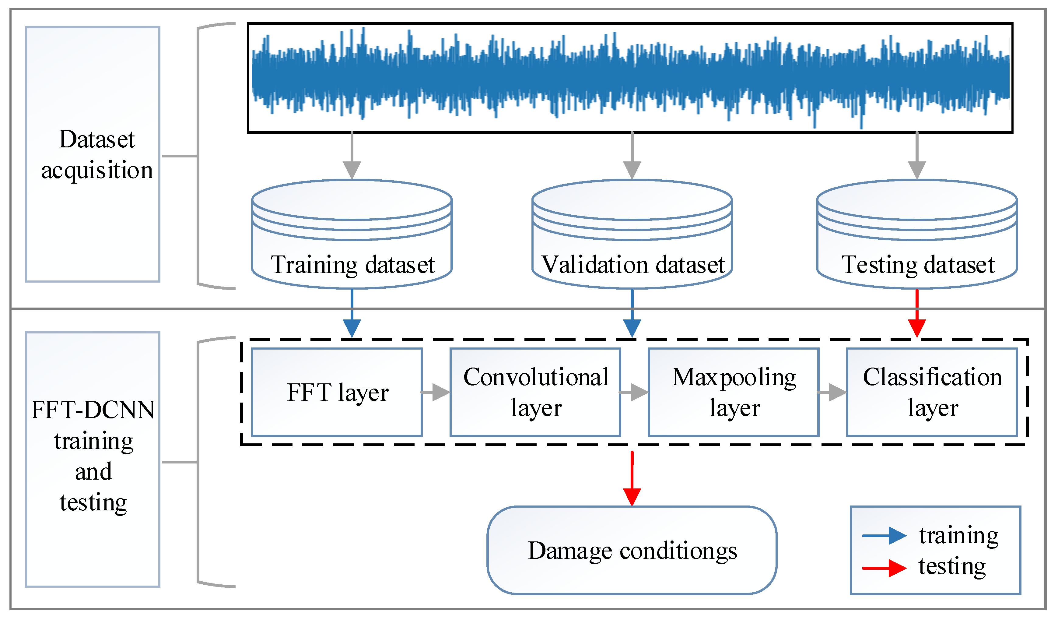
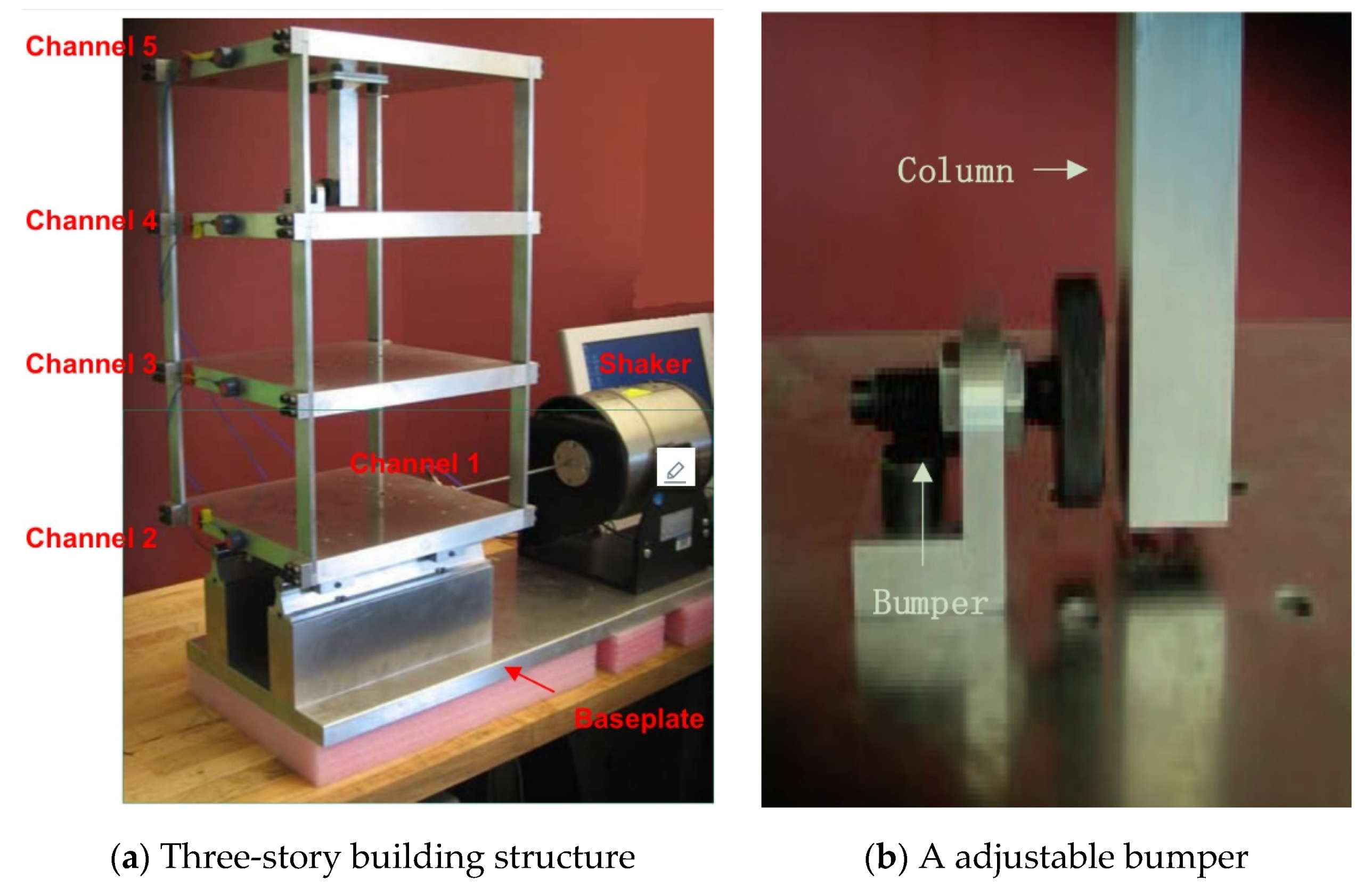
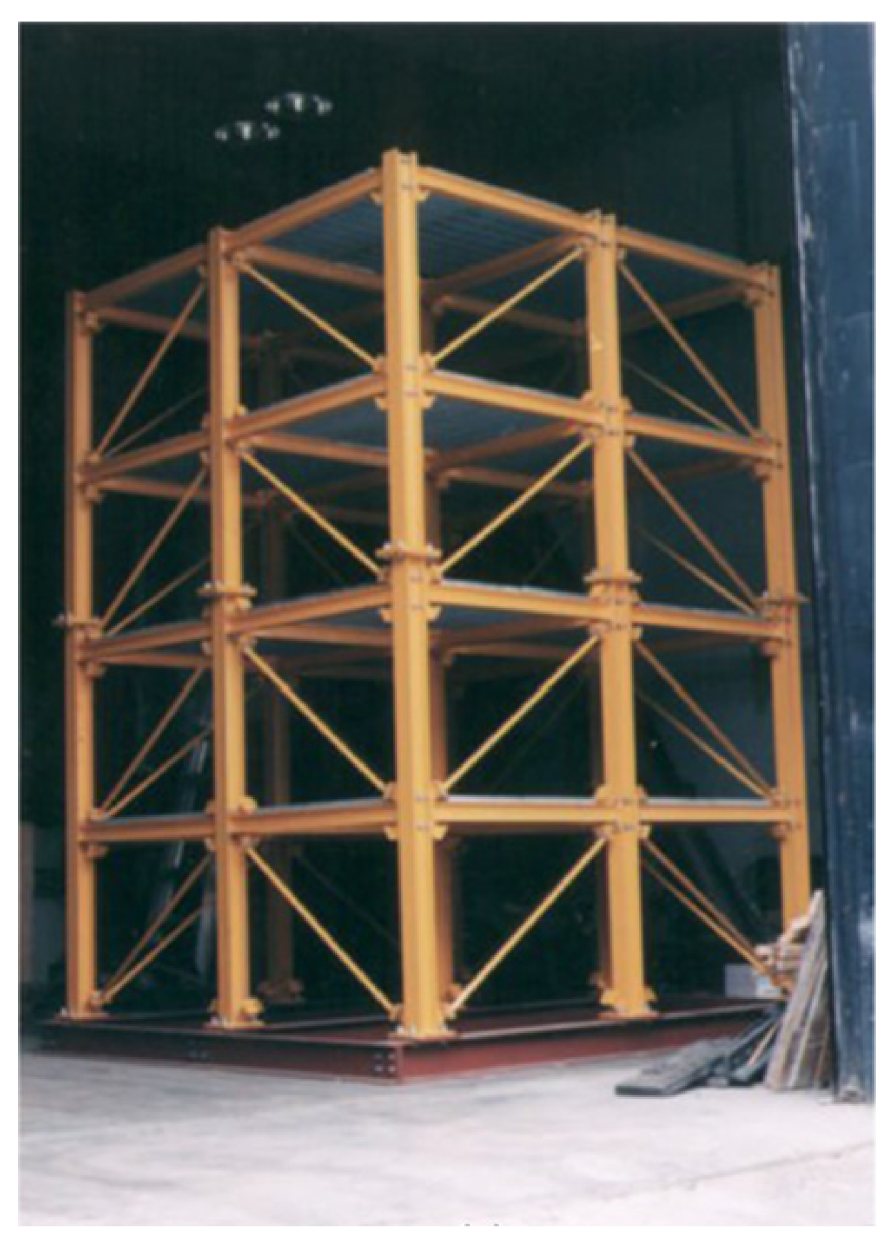
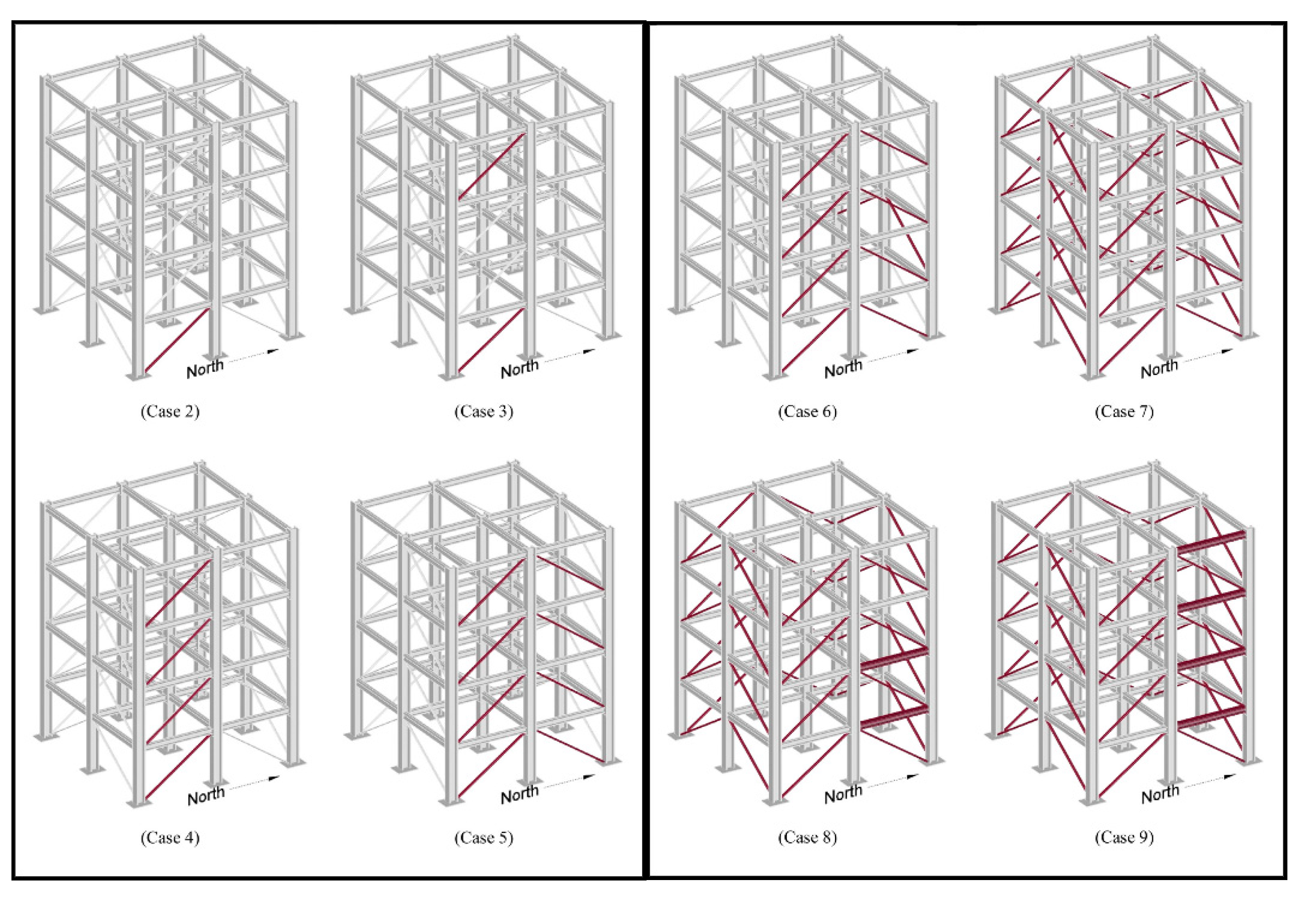
The section uses a three-story building to evaluate the effectiveness of the proposed method.

5.1. Experimental Setup and Data Description

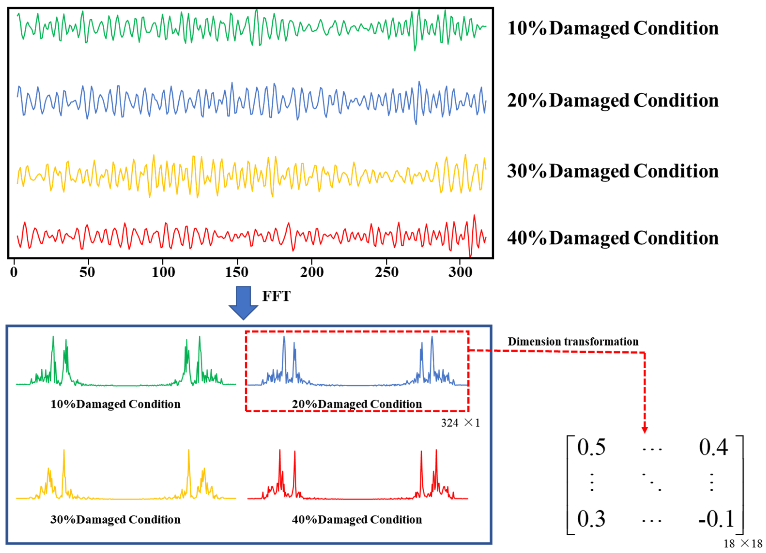
Because the sliding window length is set to 324, every one-dimensional vibration signal with 324 sampling length is obtained. The vibration signal are transformed into frequency information with 324 × 1 via FFT method. Then, frequency information is converted to $Fr{e}_M=18\times 18$ features matrix via shape dimension transformation, considering that DCNN is adopted at extracting spatial features. Finally, DCNN extracts damaged features from $Fr{e}_M$ matrix to identity structural damage. 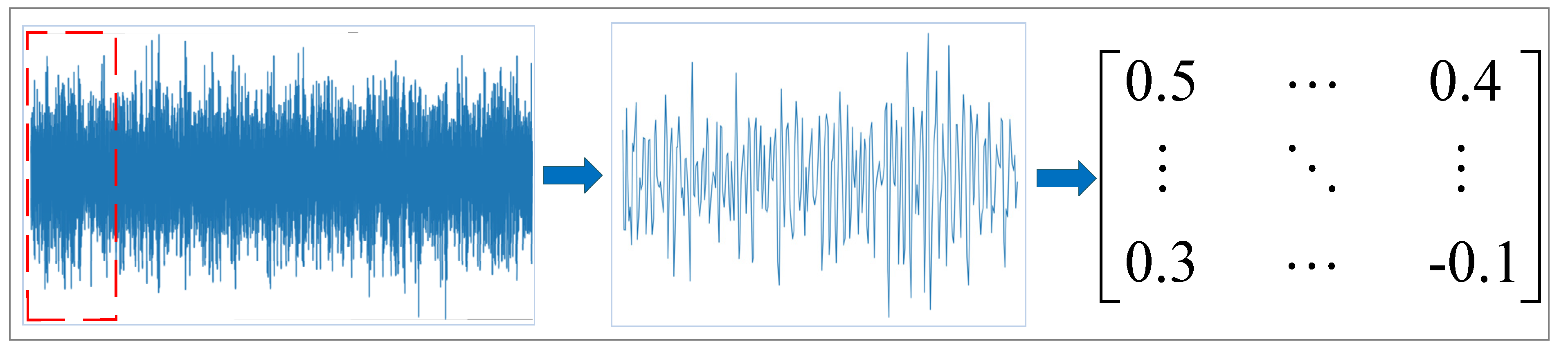Figure 6 shows the process of features transformation of four different damage condition, including that damaged degree is 10%, damaged degree is 20%, damaged degree is 30%, and damaged degree is 40%. The frequency information of different damage conditions is different with increasing damage degree.

Table 3. Parameters configuration of DCNN.

Number	Layer Name	Filter Size	Kernel Size	Stride	Padding	Output Size
First layer	Convolution 1	8	7 × 7	1 × 1	1	18 × 18
Second layer	Convolution 2	12	5 × 5	1 × 1	1	18 × 18
Third layer	Dropout 1	--	--	--	--	18 × 18
Fourth layer	Max-pooling 1	12	2 × 2	1 × 1	1	9 × 9
Fifth layer	Convolution 3	16	3 × 3	1 × 1	1	9 × 9
Sixth layer	Convolution 4	20	3 × 3	1 × 1	1	9 × 9
Seventh layer	Max-pooling 2	20	3 × 3	1 × 1	1	3 × 3

shows the configuration of the proposed method. The size of the convolutional kernel is 7 × 7 in the first layer, and the size of the convolutional kernel is 5 × 5 in the second. The maximum pooling layer is 2 × 2 in the third layer, the size of the convolutional kernel in the fourth layer is 3 × 3 in the fifth layer, and the size of the convolutional kernel is 3 × 3 in the sixth layer, and the maximum pooling layer is 2 × 2 in the seventh layer.

Table 4. Accuracy of four-fold crossvalidation.

Method	Validation (%)	Testing (%)
Fold-1	93.31	93.72
Fold-2	93.26	92.17
Fold-3	93.38	93.95
Fold-4	93.98	93.31
Mean	93.48	93.29

shows the four-fold crossvalidation result on three three-story building structures using the proposed method. In the four-fold crossvalidation, the accuracy of training datasets is 93.48% on average, and the accuracy of testing datasets is 93.29% on average. It shows that FFT-DCNN is suitable for identifying structural damage degree effectively.

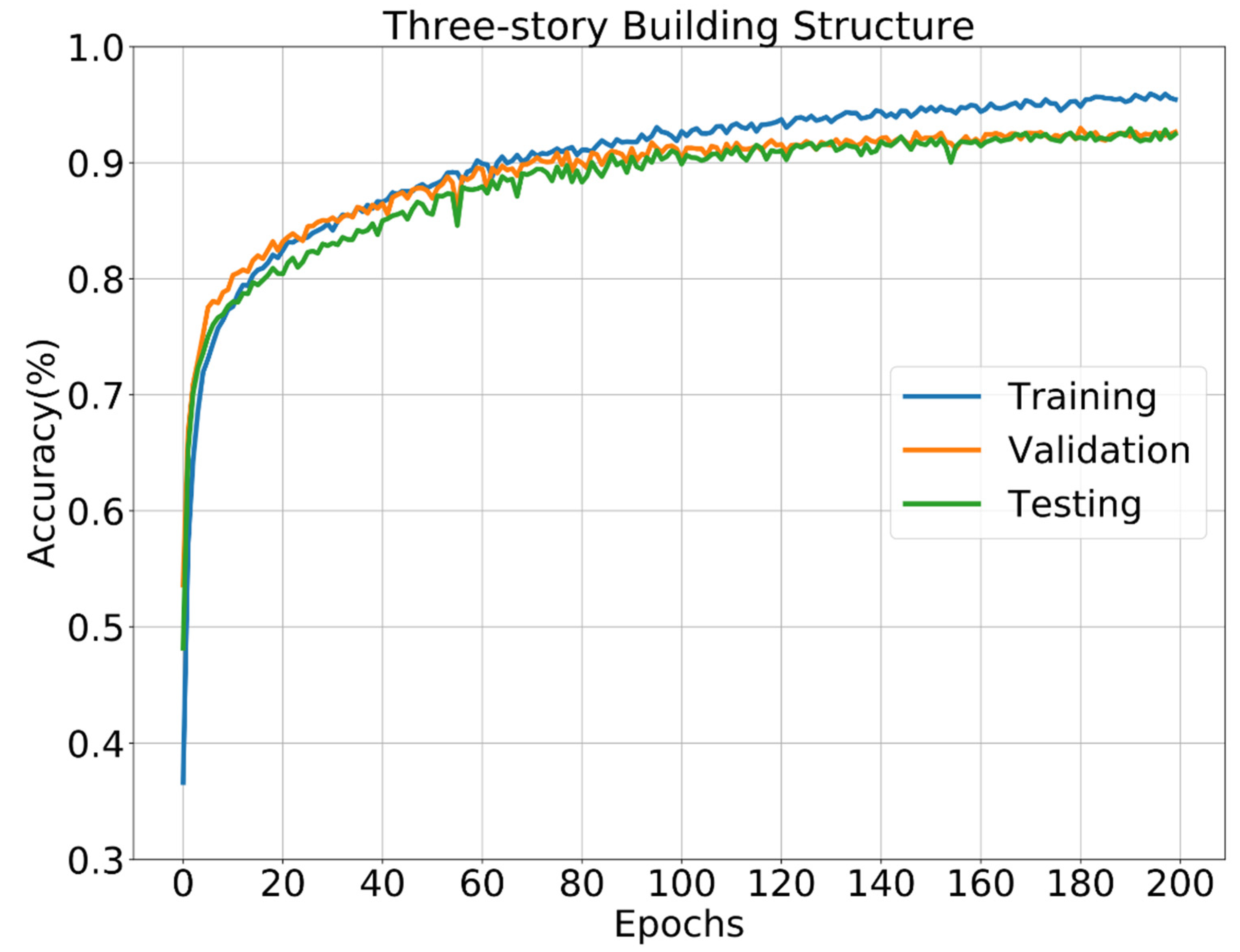
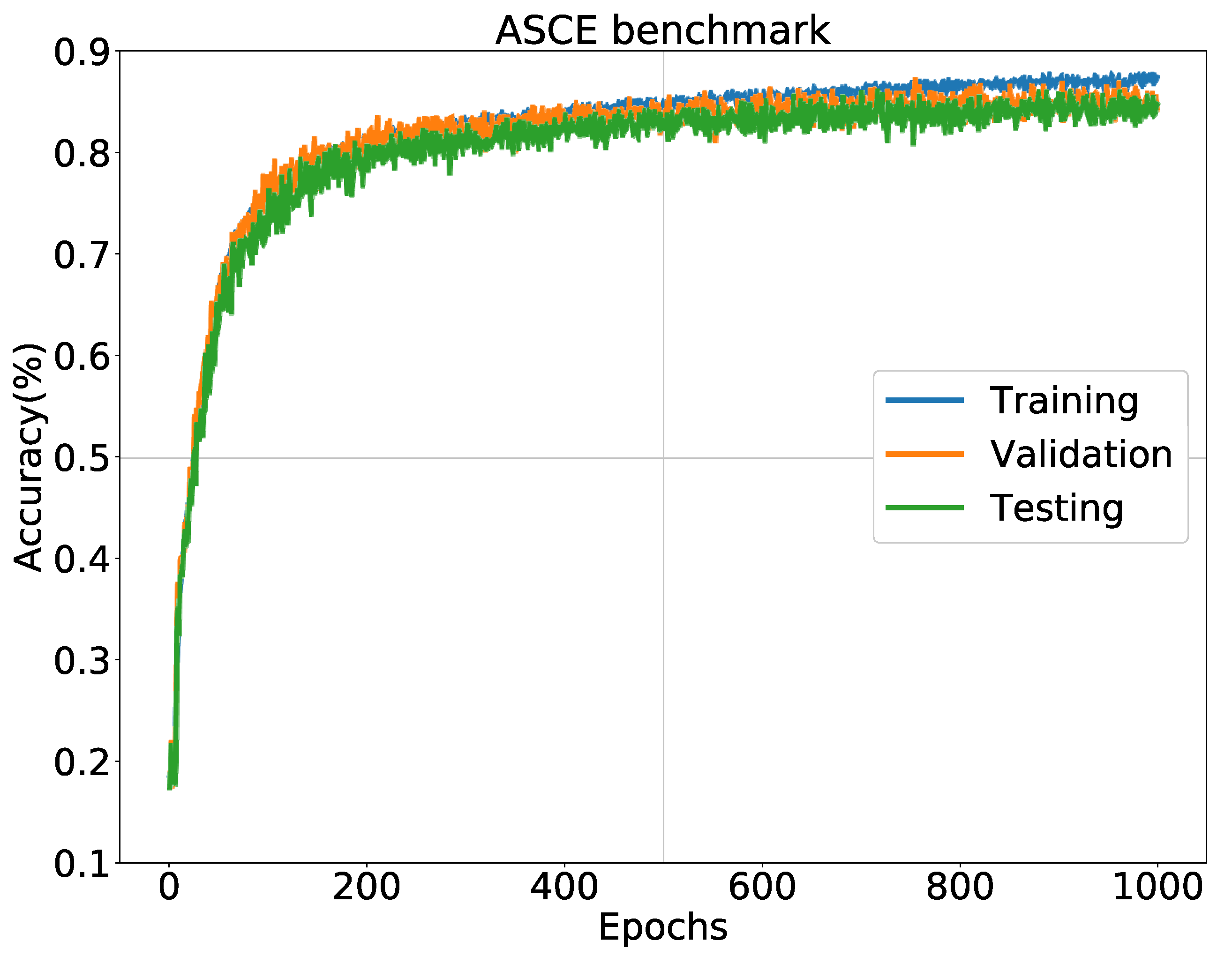
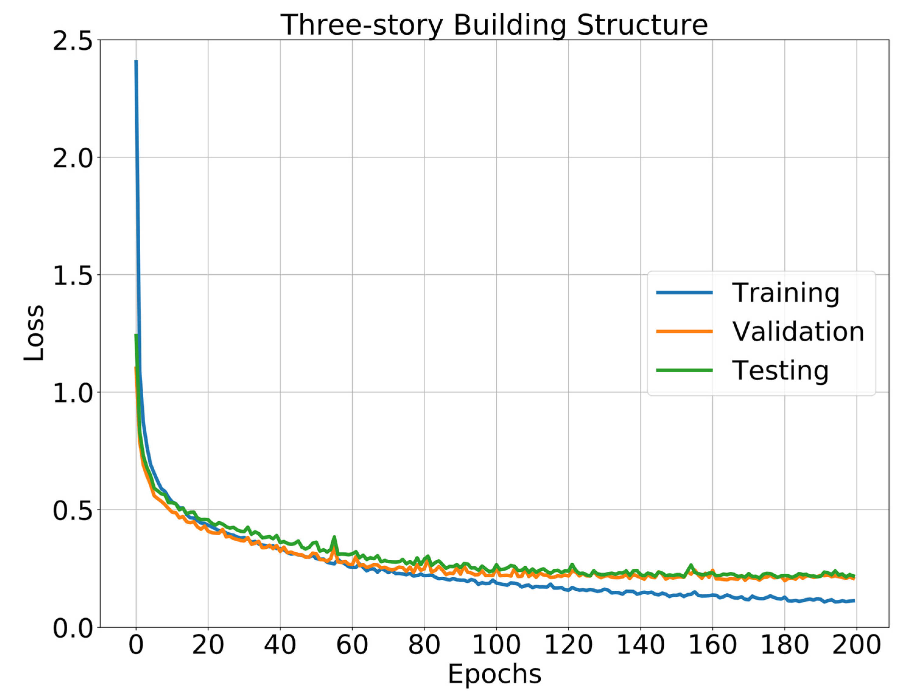
Figure 7 shows the accuracy curve for the proposed methods on Fold-1 datasets. The accuracy of training, testing, and validation reach 0.9 after achieving 200 epochs. The results show that FFT-DCNN presents an excellent ability of features extraction on the three-story building structure. In Figure 8, the loss curve of the FFT-DCNN model is smooth, which shows an excellent fitting ability and training process.

5.2. Compared with Other Methods

To verify the advantages of our proposed method, classical ML algorithms including support vector machine (SVM) [34], FFT-SVM, random forest (RF) [35], K-nearest neighbor (KNN) [36], and eXtreme gradient boosting (XGBoost) [37] are selected to evaluate structural damage degree and improved accuracy in structural damage detection. The accuracy of KNN, RF, and XGBoost is 67.64%, 70.24%, and 75.78%, respectively, representing a low ability for recognizing structural damage detection. For these algorithms, such as SVM, KNN, RF, and XGBoost, the time-sequence data of acceleration are input datasets. For FFT-DCNN and FFT-SVM algorithms, the time sequence is transformed into frequency information by the FFT method, and then frequency information is fed into DCNN or SVM algorithms. The relative setting of these algorithms are as follows:

SVM: A Gaussian RBF function is used as the SVR kernel function, and a grid search is used to determine the penalty parameters $c$ and kernel parameters $g$. The search range $c$ and $g$ are [10⁻⁴, 10⁴] and [2⁻⁴, 2⁴] by the grid searching method, respectively. Tolerance for stopping criterion is set to 1e-3, and it is enough to satisfy the error criterion.

KNN: The number of neighbors is set to 5. The value of function weights is set to uniform, representing that all points in each neighborhood are weighted equally. The power parameters. The Minkowski metric is set to 1, and it is equivalent to using Manhattan distance. The leaf size that affects the construction and query speed is set to 30.

RF: The number of trees in the forest is 100, and the maximum depth is set 3. The min samples split is set to 2, which denotes the minimum number of samples required to split an internal node. Min samples leaf represents that training samples in each of the left and right branches, and the values of Min samples leaf are set to 5. The value of Max features is set to ‘auto’, representing that the number of features to be considered when looking for the best split.

XGBoost: The maximum depth of a tree is set to 6, and the minimum child weight depth of a tree is 1. To making the update step more conservative, the max delta step is set to 0.1. L2 regularization term on weights is set 1, which can reduce the overfitting problem. The learning rate is set to 0.3. The fraction columns of random samples for each tree are set to 1.

Table 5. Comparison result between the proposed method and ML algorithms.

Method	Accuracy (%)
FFT-DCNN	93.29
FFT-SVM	90.15
SVM	85.59
KNN	67.64
RF	70.27
XGBoost	75.78

shows the comparison of damage detection ability between the algorithms mentioned above and the proposed method. It can be seen from Table 5 that the proposed method has higher accuracy in 93.38% than classical ML methods. In addition, the FFT-SVM improves accuracy by 4.56% than SVM when FFT is added to SVM. It shows that the preprocessing method, for example, FFT method, can reduce the effect of fault or noisy data and improved accuracy in structural damage detection.

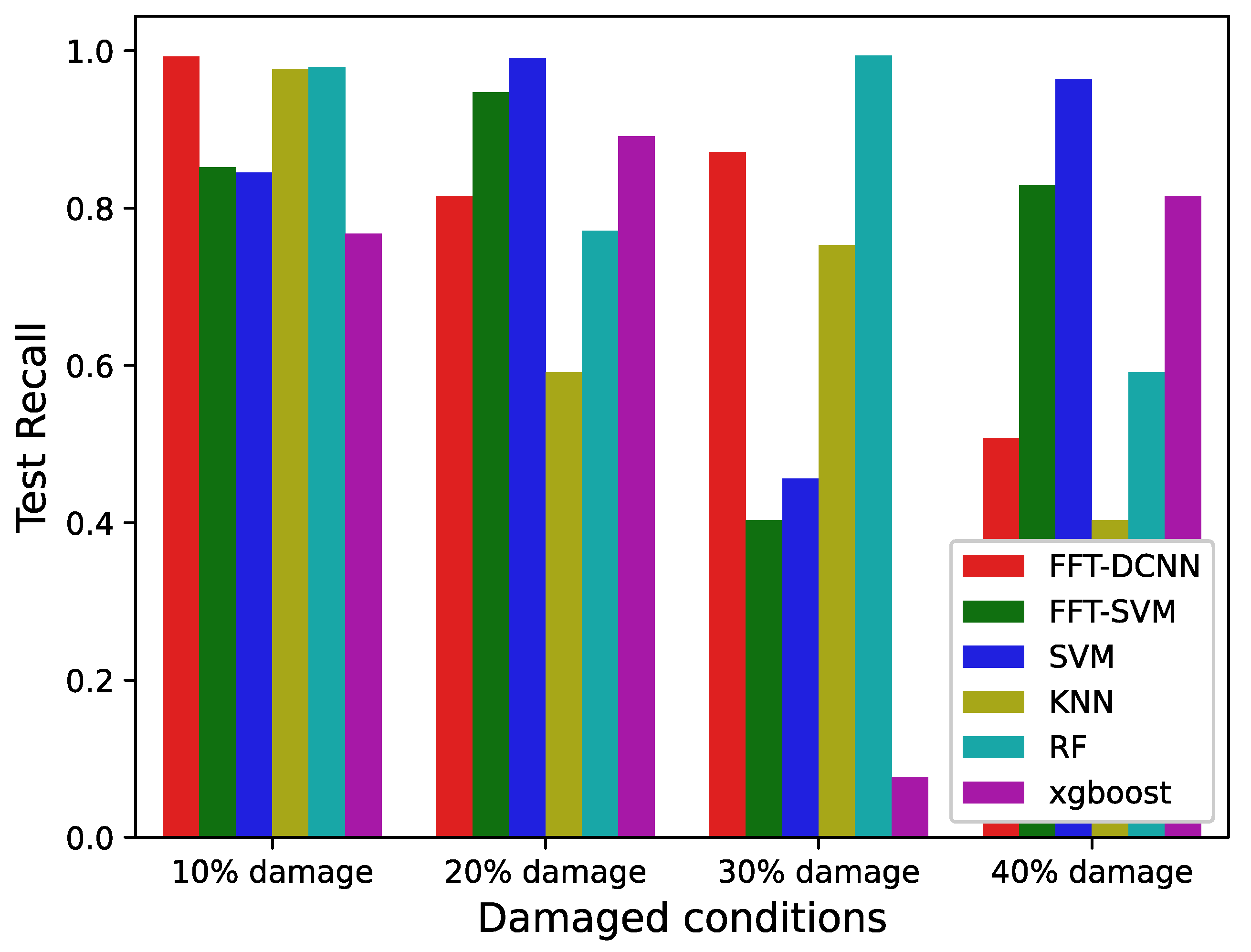
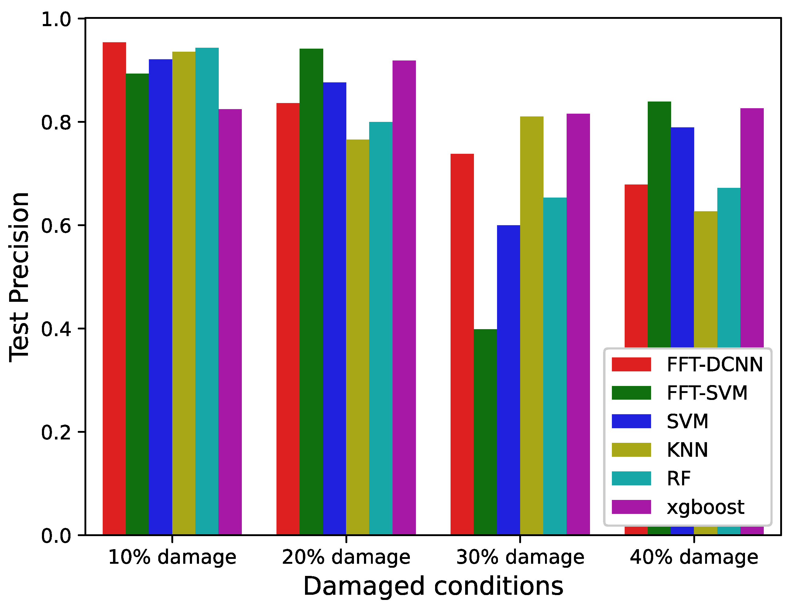
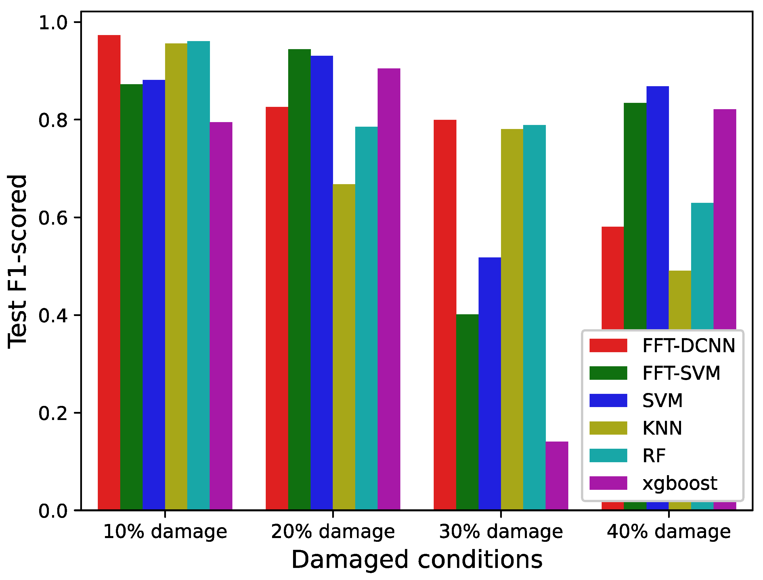
To observing the classification result of every defined pattern for test data based on different algorithms, evaluation criteria including Precision, Recall, and F₁-sore are utilized in Figure 9, Figure 10 and Figure 11. Recall represents the number of positive class predictions made out of all positive examples in the dataset. It can be seen from Figure 9 that the obtained Recall scores of 10%, 20%, and 30% damaged conditions are approximately over 0.8 using the FFT-DCNN algorithm, with the exception of 40% damaged conditions, for which the scores fall approximately 0.5. In addition, using the precision evaluating on test data, similar results are achieved for FFT-DCNN algorithm. For 10%, 20%, 30%, and 40% damaged conditions, the Precision is approximately over 0.7 with a high recognition performance, which is shown in Figure 10. It can be seen from Figure 11 that the exception of 40% damaged conditions achieves a low score, and other patterns (such as 10%, 20%, and 30% damaged conditions) obtain a high score using FFT-DCNN algorithm.

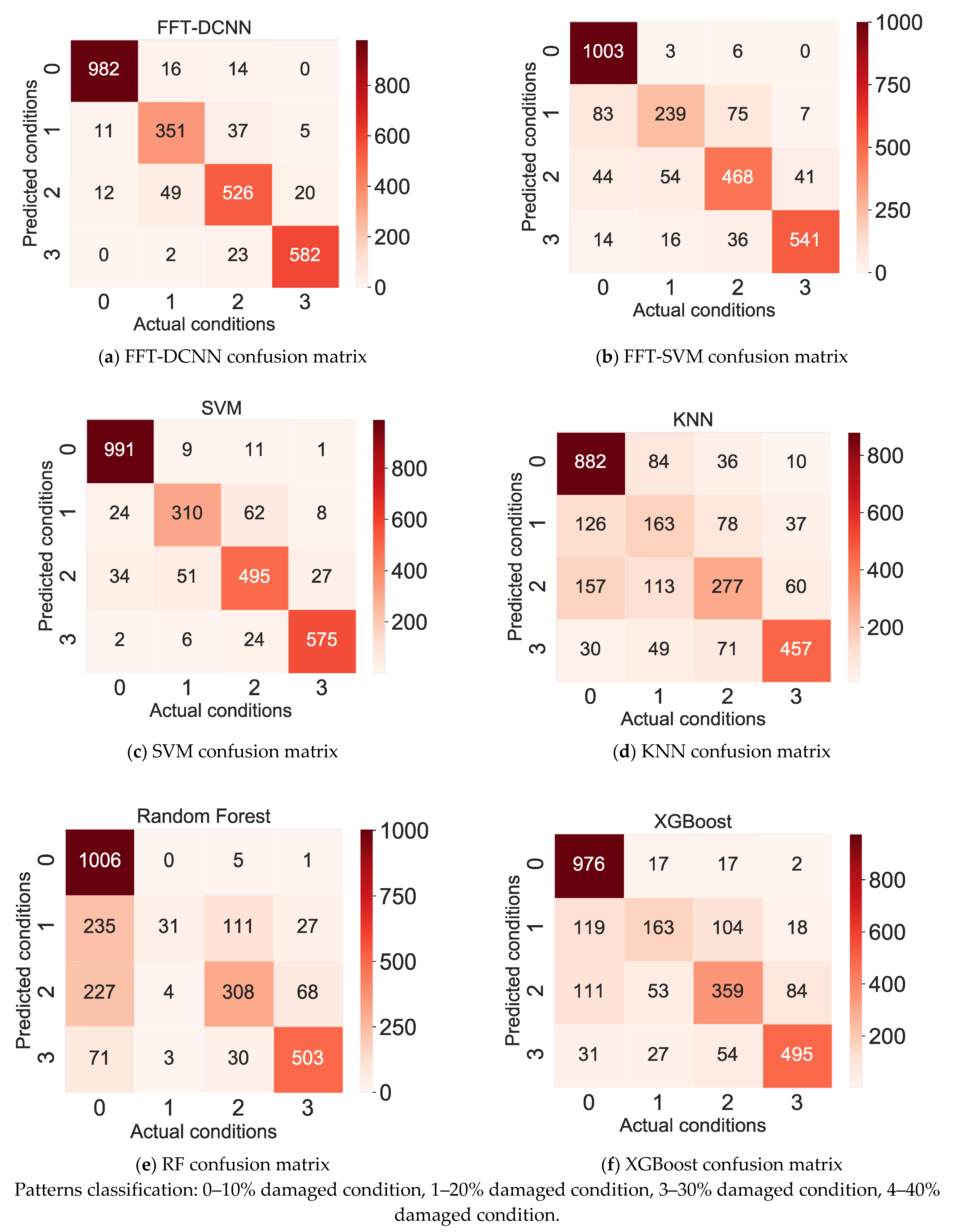
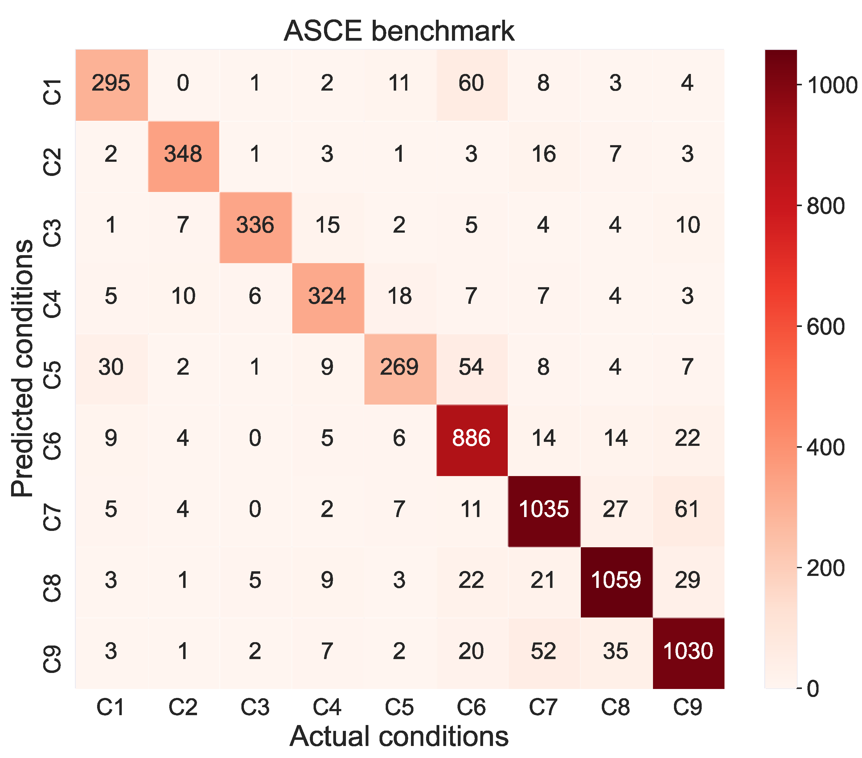
In order to reveal the classification of different algorithms under four damaged conditions of a three-story building structure, Figure 12 shows the confusion matrix of the proposed approach and compared algorithms. More specifically, in the FFT-DCNN method, the accuracy of 10% damaged condition and 40% damaged condition keep a high value over 95%. For 20% damaged condition, 37 samples are misclassified as 30% damaged condition, and 11 samples are misclassified as 10% damaged condition. The Precision keeps a high value of over 86%. The Precision is 86.7% for 30% damaged condition. Finally, the total accuracy of test data for FFT-DCNN is 93.29%, which illustrates the excellent ability of the proposed method for recognizing structural damage conditions compared with other methods, including FFT-SVM (90.15%), SVM (85.59%), KNN (67.64%), RF (70.27%), and XGBoost (75.78%). In addition, for the FFT-SVM algorithm, the numbers of classification accuracy in 0–3 damaged conditions are 1003, 239, 468, and 541, respectively, in Figure 12b. The numbers of classification accuracy in 0–3 damaged conditions are 991, 310, 495, and 575, respectively, in Figure 12c. It indicates that accuracy can be improved when the acceleration data are transformed into frequency information. More importantly, the frequency of the three-story frame generates obvious changes compared to methods based on time sequence when the structure suffers different damaged degrees. Our proposed method utilizes frequency information of three-story frame to recognize structural damage with high performance.

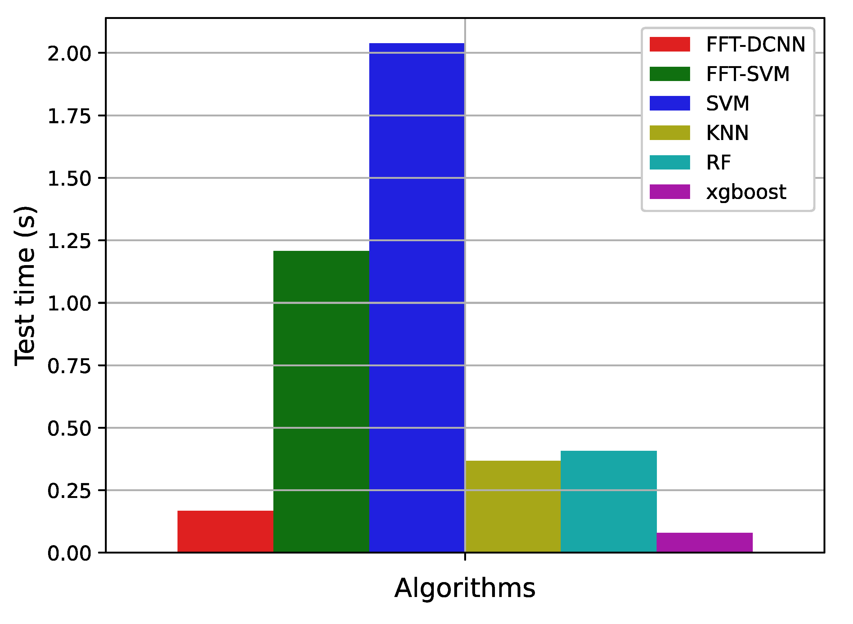
All experimental algorithms are performed in the same Windows server, and the server is configured as: GPU is GeForce RTX 3080Ti, RAM is 32 GB, and AMD Ryzen 9 5950X 16-Core Processor. It can be seen from Figure 13 and Figure 14 and

Table 6. Comparison of cost time between the proposed method and ML algorithms.

Method	Training Time (s)	Test Time (s)
FFT-DCNN	118.152	0.168
FFT-SVM	1.384	1.207
SVM	3.391	2.038
KNN	0.056	0.368
RF	5.253	0.408
XGBoost	6.754	0.079

that the proposed methods cost more time than ML algorithms during training and testing datasets. It is mainly because FFT-CNN continually updates the parameter of the network using a number of datasets. In addition, the training process finishes when the network’s loss curve begins to converge, which can cost a large amount of time in Figure 13. With the increase in computing ability, the consuming time of algorithms will be reduced in the future. Thus, the accuracy of structural damage detection should receive the primary attention, which can affect public safety.

Moreover, the test time is an important evaluation metric to judge whether the algorithm can be utilized in actual engineering. It can be seen that the proposed method takes a short time on test datasets, compared with FFT-SVM, SVM, KNN, and RF. Thus, the proposed method can be designed for recognizing structural damage in actual civil engineering.

6. Experimental Results and Discussion for ASCE Benchmark

6.1. Data Description and Experimental Setup

To verify the effectiveness of the proposed method in a complex environment, the experimental phase II of the SHM benchmark is utilized for the study. The datasets and experimental process of the ASCE benchmark were published by the American Society of Civil Engineers (ASCE) SHM task group. The height of the ASCE benchmark is 3.6 m, and the footprint dimensions are 2.5 m × 2.5 m, shown in Figure 15. The experiment aimed to provide a unified test bed for evaluating the ability of structural damage detection using different methods.

The experiment collected acceleration signals from 15 accelerometers under ambient excitation, impact hammer excitation, and 5–50 Hz randomly generated shaker excitation. Moreover, Case 1 was measured for 120 s, Case 6 was measured for 300 s, and the remaining cases were measured for 360 s. The sampling frequency for all accelerometers were set to 200 Hz. As shown in

Table 7. Description of the structural cases for the benchmark [30].

Structural Conditions	Description
Case 1	Undamaged condition
Case 2	Inclined supports located on the first floor was removed
Case 3	Inclined supports located on the first and fourth floors were removed
Case 4	Inclined supports on all floors were removed in one bay
Case 5	All inclined supports were removed on the west face
Case 6	Case 5 + inclined supports located on the second floor were removed
Case 7	All inclined supports on all faces were removed
Case 8	Loosed bolts on first and second floors of the beam + Case 7
Case 9	Loosed bolts on all floors of the beam on west face + Case 7

and Figure 16, the damaged degree was increased gradually from undamaged in Case 1 to very damaged in Case 9. Cases 2–7 removed the inclined supports at specific locations to generated structural damage, and Cases 8 and 9 loosed bolts at joint locations. In total, 31,680 samples were acquired by slicing with a window of 200 points during experimental process. Then, the dataset was divided into training, verification, and testing datasets according to the ratio of 6:2:2. That sample number for training, verification, and testing datasets are 19,008, 6336, and 6336, respectively.

6.2. FFT-DCNN Testing Result for ASCE Benchmark

The historical curve of Fold 4 is presented as an example. It can be seen from Figure 17 that there are training, testing, and validation datasets in each epoch. The accuracies of validation and testing reach 80% after Epoch 250. It indicates that the FFT-DCNN has a faster-trained process and convergence speed.

Four-fold crossvalidation results in the ASCE benchmark dataset are shown in

Table 8. Accuracy of four-fold cross-validation.

Method	Validation (%)	Testing (%)
Fold-1	87.09	86.78
Fold-2	87.93	86.38
Fold-3	88.11	87.94
Fold-4	89.12	88.10
Mean	88.06	87.30

. In each iteration, the verification accuracy is 88.06% on average, and the testing accuracy is 87.30% on average. The experimental result shows that the FFT-DCNN model is suitable for structural damage detection.

Figure 18 denotes the best result of Fold-4 for the confusion matrix. It can be seen that the label C1 is undamaged conditions, and the labels C2–C9 denote the damage conditions. The overall identification accuracy of 9 structural damage detection is 88.10%, and the error rate is 11.90%. The accuracy of C2, C6, C7, and C8 is more than 90%. C3, C4, and C9 is 88%, 84%, and 89%, respectively. While the C1 and C5 have wrong identification, but its accuracy is still over 70%, in addition, because the number of samples reaches 31,680 and it is large enough. Thus, the accuracy of FFT-CNN reaches 87.30% on average, which can satisfy the demand for structural damage detection in actual environment.

6.3. Comparative Analysis for Different Methods

The classic methods can extract sensitive features from acceleration to recognize structural damage conditions.

Table 9. Comparison result between the proposed method and ML algorithms.

Method	Accuracy (%)
FFT-DCNN	87.30
FFT-SVM	21.29
SVM	18.19
KNN	60.57
RF	71.33
XGBoost	72.80

shows the comparison between the proposed methods and classic methods. It indicates that the proposed method achieves higher performance than existing methods, including FFT-SVM, SVM, KNN, RF, and XGBoost. The experimental result shows the proposed method high identification ability in recognizing damaged conditions of civil structure.

7. Conclusions and Future Work

This study proposed a novel FFT-DCNN model to identify structural damage detection and was verified on a three-story building structure and ASCE benchmark. The main contributions of this paper are summarized as follows.

(1)

A novel data-driven method is proposed by combining FFT with DCNN, effectively handling vibration signals and accurately recognizing structural damage conditions.

(2)

Compared with traditional damage detection such as FFT-SVM and SVM, KNN, Random Forest, and XGBoost, the FFT-DCNN model automatically extracts features from the structure under different damage conditions and achieve higher accuracy in 93.38% for the three-story building structure and accuracy in 87.30% for the ASCE benchmark.

(3)

For time consumption, FFT-DCNN takes a short time on test datasets, compared with FFT-SVM, SVM, KNN, and RF. It indicates that the proposed method can be designed for recognizing structural damage in actual engineering.

(4)

This method also has some limitations. Compared with “shallow” ML methods, such as SVM and XGBoost, this method achieves high accuracy relying on a number of training datasets. Thus, we might utilize the transfer learning method to reduce training simple for accurately recognizing structural damage detection in the future.

References

1. Palma, P.; Steiger, R. Structural Health Monitoring of Timber Structures—Review of Available Methods and Case Studies. Constr. Build. Mater. 2020, 248, 118528. [Google Scholar] [CrossRef]
2. Rahul, V.; Alokita, S.; Jayakrishna, K.; Kar, V.R.; Rajesh, M.; Thirumalini, S.; Manikandan, M. Structural health monitoring of aerospace composites. In Structural Health Monitoring of Biocomposites, Fibre-Reinforced Composites and Hybrid Composites; Elsevier: Amsterdam, The Netherlands, 2019; pp. 33–52. ISBN 978-0-08-102291-7. [Google Scholar]
3. Xiang, J.; Yang, Z.; Aguilar, J. Structural Health Monitoring for Mechanical Structures Using Multi-Sensor Data. Int. J. Distrib. Sens. Netw. 2018, 14. [Google Scholar] [CrossRef] [Green Version]
4. Zhang, Z.; Sun, C. Structural Damage Identification via Physics-Guided Machine Learning: A Methodology Integrating Pattern Recognition with Finite Element Model Updating. Struct. Health Monit. 2021, 20, 1675–1688. [Google Scholar] [CrossRef]
5. Zhang, Z.; Sun, C. A Numerical Study on Multi-site Damage Identification: A Data-driven Method via Constrained Independent Component Analysis. Struct. Control. Health Monit. 2020, 27, e2583. [Google Scholar] [CrossRef]
6. Santos, A.; Figueiredo, E.; Silva, M.F.M.; Sales, C.S.; Costa, J.C.W.A. Machine Learning Algorithms for Damage Detection: Kernel-Based Approaches. J. Sound Vib. 2016, 363, 584–599. [Google Scholar] [CrossRef]
7. Chen, Z.; Tse, K.T.; Kwok, K.C.S.; Kareem, A.; Kim, B. Measurement of Unsteady Aerodynamic Force on a Galloping Prism in a Turbulent Flow: A Hybrid Aeroelastic-Pressure Balance. J. Fluids Struct. 2021, 102, 103232. [Google Scholar] [CrossRef]
8. Chen, Z.; Fu, X.; Xu, Y.; Li, C.Y.; Kim, B.; Tse, K.T. A Perspective on the Aerodynamics and Aeroelasticity of Tapering: Partial Reattachment. J. Wind Eng. Ind. Aerodyn. 2021, 212, 104590. [Google Scholar] [CrossRef]
9. Gul, M.; Catbas, F. Structural Health Monitoring and Damage Assessment Using a Novel Time Series Analysis Methodology with Sensor Clustering. J. Sound Vib. 2011, 330, 1196–1210. [Google Scholar] [CrossRef]
10. Stull, C.; Hemez, F.; Farrar, C. On Assessing the Robustness of Structural Health Monitoring Technologies. Struct. Health Monit. -Int. J. 2012, 11, 1–11. [Google Scholar] [CrossRef]
11. Seyedpoor, S.M.; Nopour, M.H. A Two-Step Method for Damage Identification in Moment Frame Connections Using Support Vector Machine and Differential Evolution Algorithm. Appl. Soft Comput. 2020, 88, 106008. [Google Scholar] [CrossRef]
12. Guo, H.Y.; Li, Z.L. Structural Damage Identification Based on Bayesian Theory and Improved Immune Genetic Algorithm. Expert Syst. Appl. 2012, 39, 6426–6434. [Google Scholar] [CrossRef]
13. Wu, J.; Guo, P.; Cheng, Y.; Zhu, H.; Wang, X.-B.; Shao, X. Ensemble Generalized Multiclass Support-Vector-Machine-Based Health Evaluation of Complex Degradation Systems. IEEE/ASME Trans. Mechatron. 2020, 25, 2230–2240. [Google Scholar] [CrossRef]
14. Ahmad, M.; Shabbir, S.; Raza, R.A.; Mazzara, M.; Distefano, S.; Khan, A.M. Artifacts of Different Dimension Reduction Methods on Hybrid CNN Feature Hierarchy for Hyperspectral Image Classification. Optik 2021, 246, 167757. [Google Scholar] [CrossRef]
15. Jia, S.; Jiang, S.; Lin, Z.; Li, N.; Xu, M.; Yu, S. A Survey: Deep Learning for Hyperspectral Image Classification with Few Labeled Samples. Neurocomputing 2021, 448, 179–204. [Google Scholar] [CrossRef]
16. Lauriola, I.; Lavelli, A.; Aiolli, F. An Introduction to Deep Learning in Natural Language Processing: Models, Techniques, and Tools. Neurocomputing 2021. [Google Scholar] [CrossRef]
17. Gulgec, N.S.; Takáč, M.; Pakzad, S.N. Convolutional Neural Network Approach for Robust Structural Damage Detection and Localization. J. Comput. Civ. Eng. 2019, 33, 04019005. [Google Scholar] [CrossRef]
18. Tang, Z.; Chen, Z.; Bao, Y.; Li, H. Convolutional Neural Network-Based Data Anomaly Detection Method Using Multiple Information for Structural Health Monitoring. Struct Control. Health Monit 2019, 26, e2296. [Google Scholar] [CrossRef] [Green Version]
19. Abdeljaber, O.; Avci, O.; Kiranyaz, M.S.; Boashash, B.; Sodano, H.; Inman, D.J. 1-D CNNs for Structural Damage Detection: Verification on a Structural Health Monitoring Benchmark Data. Neurocomputing 2018, 275, 1308–1317. [Google Scholar] [CrossRef]
20. Zhang, Y.; Miyamori, Y.; Mikami, S.; Saito, T. Vibration-based Structural State Identification by a 1-dimensional Convolutional Neural Network. Comput.-Aided Civil. Infrastruct. Eng. 2019, 34, 822–839. [Google Scholar] [CrossRef]
21. Hoshyar, A.N.; Samali, B.; Liyanapathirana, R.; Houshyar, A.N.; Yu, Y. Structural Damage Detection and Localization Using a Hybrid Method and Artificial Intelligence Techniques. Struct. Health Monit. 2020, 19, 1507–1523. [Google Scholar] [CrossRef]
22. Amini Tehrani, H.; Bakhshi, A.; Akhavat, M. An Effective Approach for Structural Damage Localization in Flexural Members Based on Generalized S-Transform. Sci. Iran. 2017. [Google Scholar] [CrossRef]
23. Nguyen, T.Q. A Data-Driven Approach to Structural Health Monitoring of Bridge Structures Based on the Discrete Model and FFT-Deep Learning. J. Vib. Eng. Technol. 2021. [Google Scholar] [CrossRef]
24. Fan, N.; Balan, R.V.; Rosca, J. Comparison of Wavelet- and FFT-Based Single-Channel Speech Signal Noise Reduction Techniques; Truchetet, F., Laligant, O., Eds.; International Society for Optics and Photonics: Philadelphia, PA, USA, 2004; pp. 127–138. [Google Scholar]
25. Gopinathan, S.; Kokila, R.; Thangavel, P. Wavelet and FFT Based Image Denoising Using Non-Linear Filters. IJECE 2015, 5, 1018. [Google Scholar] [CrossRef]
26. Zheng, J.; Liao, L.; Chen, Y. Damage Identification Based on Convolutional Neural Network and Recurrence Graph for Beam Bridge. Struct. Health Monit. 2020. [Google Scholar] [CrossRef]
27. Malek, S.; Melgani, F.; Bazi, Y. One-Dimensional Convolutional Neural Networks for Spectroscopic Signal Regression: Feature Extraction Based on 1D-CNN Is Proposed and Validated. J. Chemom. 2018, 32, e2977. [Google Scholar] [CrossRef]
28. Hung, D.V.; Hung, H.M.; Anh, P.H.; Thang, N.T. Structural Damage Detection Using Hybrid Deep Learning Algorithm. STCE 2020, 14, 53–64. [Google Scholar] [CrossRef] [Green Version]
29. Pan, H.; Gui, G.; Lin, Z.; Yan, C. Deep BBN Learning for Health Assessment toward Decision-Making on Structures under Uncertainties. KSCE J. Civ. Eng. 2018, 22, 928–940. [Google Scholar] [CrossRef]
30. Dyke, S.J.; Bernal, D.; Beck, J.; Ventura, C. Experimental Phase II of the Structural Health Monitoring Benchmark Problem. Lakartidningen 2003, 105, 2239–2240. [Google Scholar]
31. Lin, Y.; Nie, Z.; Ma, H. Structural Damage Detection with Automatic Feature-Extraction through Deep Learning: Structural Damage Detection with Automatic Feature-Extraction through Deep Learning. Comput.-Aided Civil. Infrastruct. Eng. 2017, 32, 1025–1046. [Google Scholar] [CrossRef]
32. Wu, H.; Gu, X. Towards Dropout Training for Convolutional Neural Networks. Neural Netw. 2015, 71, 1–10. [Google Scholar] [CrossRef] [Green Version]
33. Fan, Z.; Li, C.; Chen, Y.; Mascio, P.D.; Chen, X.; Zhu, G.; Loprencipe, G. Ensemble of Deep Convolutional Neural Networks for Automatic Pavement Crack Detection and Measurement. Coatings 2020, 10, 152. [Google Scholar] [CrossRef] [Green Version]
34. Gui, G.; Pan, H.; Lin, Z.; Li, Y.; Yuan, Z. Data-Driven Support Vector Machine with Optimization Techniques for Structural Health Monitoring and Damage Detection. KSCE J. Civ. Eng. 2017, 21, 523–534. [Google Scholar] [CrossRef]
35. Lei, X.; Sun, L.; Xia, Y.; He, T. Vibration-Based Seismic Damage States Evaluation for Regional Concrete Beam Bridges Using Random Forest Method. Sustainability 2020, 12, 5106. [Google Scholar] [CrossRef]
36. Vitola, J.; Pozo, F.; Tibaduiza, D.; Anaya, M. A Sensor Data Fusion System Based on K-Nearest Neighbor Pattern Classification for Structural Health Monitoring Applications. Sensors 2017, 17, 417. [Google Scholar] [CrossRef] [PubMed]
37. Leon-Medina, J.X.; Anaya, M.; Parés, N.; Tibaduiza, D.A.; Pozo, F. Structural Damage Classification in a Jacket-Type Wind-Turbine Foundation Using Principal Component Analysis and Extreme Gradient Boosting. Sensors 2021, 21, 2748. [Google Scholar] [CrossRef]
Figure 1. Architecture of the proposed method.
Applsci 11 09345 g001
Figure 2. Flowchart of features extraction.
Applsci 11 09345 g002
Figure 3. Flowchart of the proposed FFT-DCNN for structural damage detection.
Applsci 11 09345 g003
Figure 4. Experimental setup of the building structure.
Applsci 11 09345 g004
Figure 5. K-fold crossvalidation method.
Applsci 11 09345 g005
Figure 6. Vibration signal decomposition via FFT method.
Applsci 11 09345 g006
Figure 7. Training accuracy history of the FFT-DCNN algorithm.
Applsci 11 09345 g007
Figure 8. Training loss history of the FFT-DCNN algorithm.
Applsci 11 09345 g008
Figure 9. Recall of the test data using different algorithms.
Applsci 11 09345 g009
Figure 10. Precision of the test data using different algorithms.
Applsci 11 09345 g010
Figure 11. F1-scored of the test data using different algorithms.
Applsci 11 09345 g011
Figure 12. Confusion matrix between actual conditions and predicted conditions.
Applsci 11 09345 g012
Figure 13. Comparison of training time between the proposed method and ML algorithms.
Applsci 11 09345 g013
Figure 14. Comparison of test time between the proposed method and ML algorithms.
Applsci 11 09345 g014
Figure 15. Four-story structure of ASCE benchmark.
Applsci 11 09345 g015
Figure 16. Structural damaged condition 2–9 of ASCE benchmark. (Red color denotes removed inclined supports locations or loosed bolts).
Applsci 11 09345 g016
Figure 17. Confusion matrix of damage identification for Fold 4.
Applsci 11 09345 g017
Figure 18. Confusion matrix of damage identification for the Fold-4.
Applsci 11 09345 g018