Article

Design, Construction and Validation of a Proof of Concept Flexible–Rigid Mechanism Emulating Human Leg Behavior

Department of Electrical and Computer Engineering, University of California Santa Cruz, Santa Cruz, CA 95064, USA
*
Author to whom correspondence should be addressed.
Current address: 1156 High Street, Santa Cruz, CA 95064, USA.
These authors contributed equally to this work.
Submission received: 10 August 2021 / Revised: 16 September 2021 / Accepted: 21 September 2021 / Published: 8 October 2021
(This article belongs to the Section Robotics and Automation)

Abstract

:
In most robotics simulations, human joints (e.g., hips and knees) are assumed to be revolute joints with limited range rotations. However, this approach neglects the internal flexibility of the joint, which could present a significant drawback in some applications. We propose a tensegrity-inspired robotic manipulator that can replicate the kinematic behavior of the human leg. The design of the hip and knee resembles the musculoskeletal connections within the human body. Our implementation represents muscles, tendons and ligament connections as cables, and bones as rods. This particular design manipulates muscles to replicate a human-like gait, which demonstrates its potential for use as an anatomically correct assistive device (prosthetic, exoskeleton, etc.). Using the OpenSim 3.0 simulation environment, we estimated the kinematics and structural integrity of the proposed flexural joint design and determined the actuation strategies for our prototype. Kinematics for the prototype include the mechanical limitations and constraints derived from the simulations. We compared the simulation, physical prototype, and human leg behaviors for various ranges of motion and demonstrated the potential for using OpenSim 3.0 as a flexible–rigid modeling and simulation environment.

1. Introduction

The human body consists of a musculoskeletal system to facilitate locomotion. This system is composed of rigid and flexible components such as bones, muscles, tendons, and ligaments to distribute stresses and maintain structural integrity [1,2,3] to respond to external stimuli (e.g., forces).
Most robotic systems are either rigid to maximize load bearing [4,5], or soft to optimize compliance to the environment or promote soft interactions [6,7]. Rigid manipulators often consist of revolute joints with stiff linkages, which are suitable for precise movements (e.g., industrial manufacturing robots); however, they can be structurally damaged by sudden impacts [8,9]. Soft robots distribute strain and load throughout the system adapting better to unpredictable conditions (e.g., uneven terrain, unexpected impacts). A crucial limitation is the lack of a rigid support structure that lowers the load carrying capacity of the robot [10,11,12]. The compromise solution often applied in assistive robotics connects rigid structural elements using compliant joints [13], or actuators [14].
An example of this hybrid system is a tensegrity structure, which consists of rigid compression components suspended in a network of flexible tension elements that distribute stress and strain throughout the system. A tensegrity structure can withstand load while maintaining the flexibility and adapting to unpredictable events [2,15,16]. It was shown that tensegrity robots could locomote by shifting their centers of gravity [17,18], contracting and expanding their structure [19] or mimicking biological locomotion [20]. It was also shown that they could mimic human spine [21,22], arms [23,24], knees [25] and legs [26].
One of the first representations of a functional human body tensegrity-inspired manipulator was proposed by Graham Scarr [27]. This concept uses two rigid and several tensile elements interconnected into a tensegrity structure to replicate aspects of the functionality of a human elbow joint. Baltaxe et al. [24], Lessard et al. [28], Jung et al. [26] and Castro et al. [25] proposed several concept manipulators that replicate the behavior of elbow, shoulder and knee joints. The robotic configuration proposed here is designed to create a gait-inspired motion. Figure 1 schematically shows the physical model comprised of a “hip” joint (Figure 2) and a “knee” joint (Figure 3). The interconnected web of passive and active tensile components mimic the biological tendon and ligament connections ensuring system compliance, while preventing direct contact between the rigid components. The proposed design uses three active tensile elements (inspired by the hamstring, iliopsoas, and gluteus maximus muscles) to complete a full cycle of hinged human gait along the sagittal plane.
Several simulation solutions for tensegrity-inspired structures were proposed. NASA Tensegrity Robotics Toolkit (NTRT) [29] simulates and controls the behavior of a tensegrity structure using C++ and MATLAB modules interfaced with a Bullet Physics Engine [30], which was originally developed for video game animations and movies visual effects. The main advantage of using a video game engine for simulating the dynamic behavior or robotics structures is the simulation speed. Bullet is a GPU-based simulation tool; the main disadvantage of this approach is that game engine solvers are primarily focussed on the visual effect instead of the mathematiocal accuracy of the simulation. Modeling of Tensegrity Structures (MOTES) [31] is a MATLAB simulation package optimized for static analysis that determines the failure criteria using non-linear optimization solver. It has been shown that ABAQUS can be used to predict the stress–strain relationship of three dimensional tensegrity structures [32]. MOTES and ABAQUS are limited to static analysis, and we concluded OpenSim 3.0 provided kinematic and dynamic analysis that allows us to bridge robotic and human models.
The obotic manipulator presented here uses as a starting point the design developed by Jung et al. [26]. The current design proposes an improved mechanical structure and sensing strategy (e.g., IMU localization for monitoring the manipulator’s dynamic behavior). One of the main contributions of the paper is the pipeline that combines the physical prototype and human subject in the same environment. This approach could be used for streamlining the development of future flexible mechanisms. In this paper, we propose a methodology to develop flexible–rigid robots with a dynamics behavior equivalent to musculoskeletal systemsdevelop a flexible–rigid robotic system that replicates the musculoskeletal connections within the human leg and can replicate aspects of the human leg kinematic and dynamic behavior. The model is developed in the OpenSim 3.0 environment (an open source modeling platform for biomechanical modeling, simulation and analysis [33,34,35]) to validate an experimental tensegrity-inspired robot designed and fabricated in-house (Figure 4). Section 2 shows the custom flexible–rigid prototype design process. Section 3 explains the OpenSim 3.0 environment and discusses the model-based dynamics that generate kinematic movements. We developed the robotic manipulator and the OpenSim model at the same time. The goal was for the model to inform the structural design and, therefore, predict its dynamic behavior. Section 4 describes the control and actuation strategies. Section 5 discusses the experimental validation. Section 6 concludes the paper.

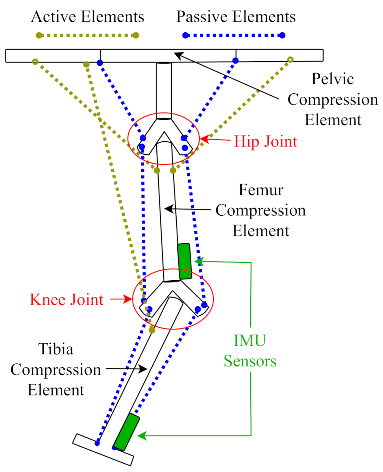
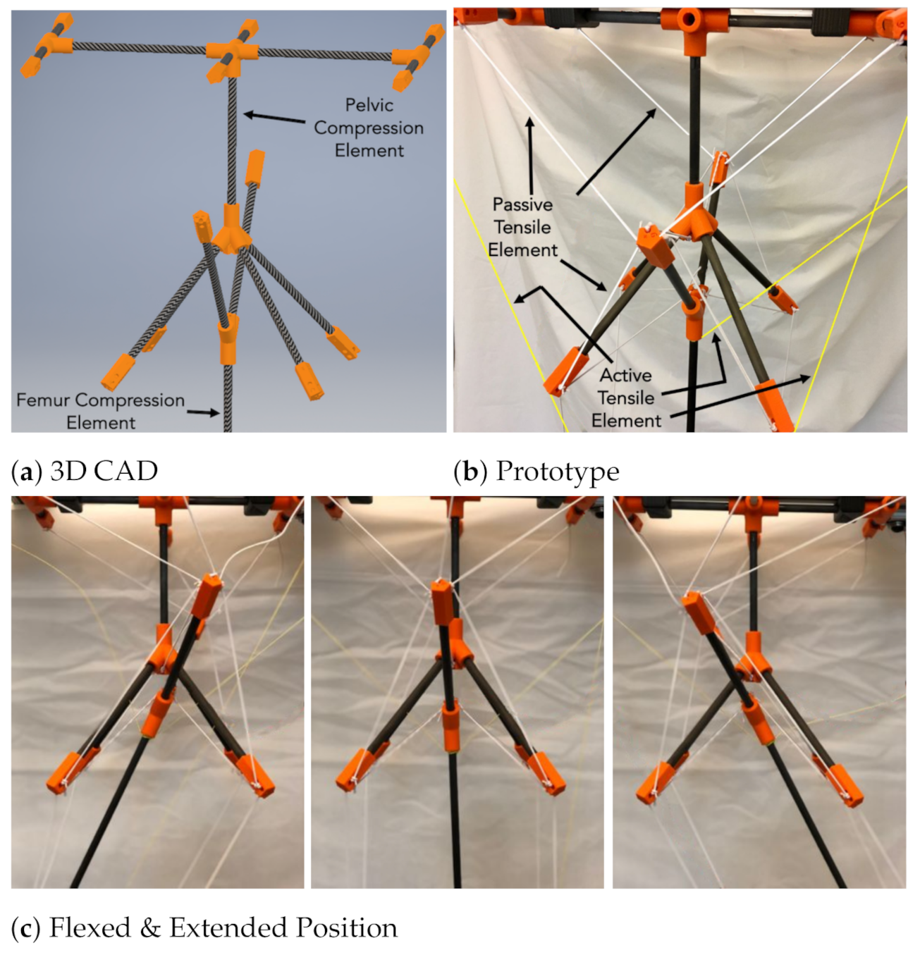
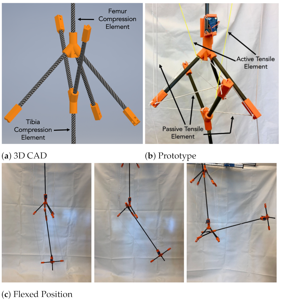
2. Structural Design

2.1. Compression Elements

The design consists of three main rigid elements representing the human pelvic bone, the femur and the tibia (Figure 1). The compression elements are carbon fiber rods assembled with 3D-printed acrylonitrile butadiene styrene (ABS) pieces. The length of the compression elements were chosen to match the dimensions of the bones in the OpenSim 3.0 model Gait2345_Simbody described in []Section IIthe Simulation Modeling Section. In Figure 1, the upper compression element is equivalent to a human pelvic bone, the middle element mimics a femur bone, and the lowest segment acts as the tibia and fibula, simplified into one rigid body. The hip joint performs similar to a ball and socket joint, which is not confined to one axis of rotation like most conventional robotic joint designs (Figure 2a,b). The knee joint has a dominant degree of freedom during flexing using a single actuating muscle, which resembles the biological biceps femoris (Figure 3a,b).
The flexural joints are secured by a complex network of tensile components that perform similarly to muscles and other tendon-based bone-element connections [26]. To achieve multi-axis compliance, the Y-shape design for the femur and tibia compression elements (Figure 2) is capable of generating flexion, extension, adduction, and abduction motion. The positional displacement of the tensegrity flexural hip joint produces a lifting motion advancing the structure to begin gait (see Figure 2). The tibia compression element is attached to a three-rod base, designed similarly to the patella and femur. It creates a flexural knee joint that flexes along one axis of rotation (as shown in Figure 3). When the cable-driven actuator shortens the hamstring, it pulls the tibia segment to flex the knee joint. This also pulls the femur, allowing the structure to maneuver and provide one fluid gait motion.

2.2. Tensile Elements

In tensegrity structures, the tensile elements maintain stability and achieve characteristics similar to muscles, ligaments and tendons [26]. Here, we used bungee cords for the passive tensile elements and fish-line spectra cord for the active ones. Passive tensile elements distribute forces upon impact and maintain structural compliance in response to external events. Each active cable has an antagonistic cable, which lengthens and relaxes, similar to how muscles contract and extend. The tensegrity manipulator contains sixteen pairs of antagonistic passive elements (six in the hip, and ten in the knee), which deform due to the applied force, then return the leg to its equilibrium position. Pre-tensioned passive cables allow the tensegrity structure to return to its original shape. Active tensile elements allow the structure to create motion similar to the human leg and generate human-like gaits.

2.3. Joint Design

The most prominent active muscles throughout one cycle of in-place gait are are the hamstring, iliopsoas and gluteus maximus [36,37]. Normal gait requires a complex design and, due to this being a proof of concept tensegrity-inspired design, we focused our attention on aligning the biomechanics and robotic manipulators within the same system to prove that it is capable of more. The behavior of this manipulator was comparable to a suspended human leg performing in-place gait and was never intended to carry a load. Our model has an equivalent cable-driven actuator for each muscle one of them. Figure 2 and Figure 3 show the “hip” and “knee” joints. The 3D printed connections in orange (Figure 2a and Figure 3a), work similarly to a puzzle, where prototype extrusions are assembled to create a multi-body system. The actuators positioned at one end of the active tensile elements annotated in Figure 1, while the rest of the passive tensile components create a complex network of cables holding the system together.
For easier manipulation and to match the geometry of the simulated structure, the Y-shaped pieces have through holes for the actuating cables. The active–passive pairs of tensile elements support the structure and prevent direct contact between the compression elements.

2.4. Directed Cable Routing

Each cable is actuated by a dedicated motor, which can either turn in one direction to tighten the cable or in the opposite direction to loosen it to generate a gait-inspired motion. The cable-driven actuator acts similarly with the iliopsoas (front hip motor) and pulls the femur-inspired element forward. The antagonistic active tensile element to the iliopsoas, the gluteus maximus (back hip motor), moves the structure back, to produce a follow-through motion. The bicep femoris long-head (hamstring motor) is essential in emulating human knee flexion. Although this initial prototype robotic manipulator was not intended to stand on its own, similar to the human hip, the two cables on the femur emulate an action similar to walking.

2.5. Actuator Selection

Cable-driven actuators shorten the cables to resemble muscle contractions and perform knee flexion and hip swings. The location of the actuators is critical for applying the optimal forces and actuation patterns (Figure 5) on the deforming structure while minimizing the power consumption and found when simulating the model. Figure 6A shows the predicted forces necessary to actuate the structure during a full gait cycle. To maximize the torque to weight ratio we select three Polou 3454 DC motors that have a 100:1 gear ration and 0.64 Nm stall torque (the largest predicted force is 100N, which translates to a 0.44 Nm applied torque). Varying the size of the models (50% Scaled, Unscaled, and 150% Scaled in Figure 6) within the simulation guided the hardware requirements. The power consumption of the OpenSim 3.0 simulated robot was computed using the ProbeReport and the JointInternalPowerProbe analysis [38].

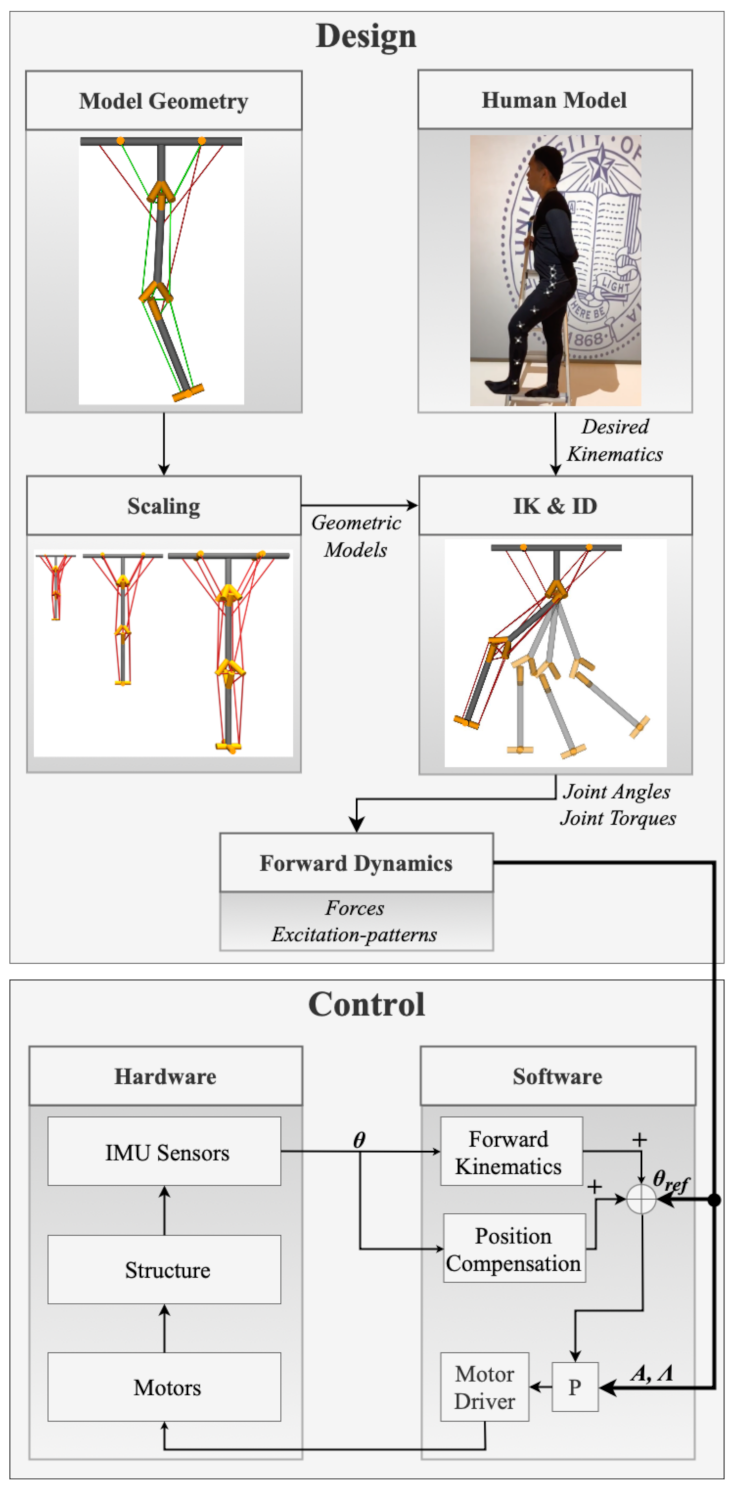
3. Simulation Modeling

OpenSim 3.0 [33] biomechanics simulation and analysis environment was used to predict the forces and ranges of motion. The Gait2345_Simbody model was adapted by altering the file and removing components (e.g., bones, muscles, etc.) to a suspended human leg to reproduce a target hinged gait pattern with similar constraints as the physical model. Each configuration and marker set file was imported into the Scaling Tool (Figure 4) to generate different sized models (e.g., varying lengths, masses, etc.)easily adapt to different sized users and models (e.g., varying lengths, masses, etc.). The Scaling Tool matched the physical prototype and the participant according to the reflective infrared markers placed on both subjects with mm precision. The calibration process required a static file with markers that match the same placement on the simulated model and the physical subject. The Forward Dynamics (FD) tool was used to solve the system’s governing dynamic equations that integrate the model’s musculoskeletal dynamical equations, which could be expressed for each muscle as:
  • Moments due to muscle forces: τ m = [ R ( q ) ] f ( a , l , l ˙ )
  • Muscle contraction rate: l ˙ = Λ ( a , l , q , q ˙ )
  • Muscle activation rate: a ˙ = A ( a , x )
where τ m is the net muscle moment, [ R ( q ) ] is the moment arm for the position q, f is the muscle force, a is muscle activation value, l is the muscle fiber length, x is the model controls parameter. FD demonstrated that with any experimental set of motions, the resulting muscle activations yield similar kinematic results to other available tools as well as control techniques for robotic manipulators. The equation of motion is:
q ¨ = [ M 1 ( q ) ] { τ C ( q , q ˙ ) G ( q ) } ]
where q, q ˙ and q ¨ are the positions, velocities and accelerations. [ M 1 ( q ) ] represents the inverse of the mass matrix, τ is the vector of generalized forces, C ( q , q ˙ ) is the vector of Coriolis and centrifugal forces, and G ( q ) is the vector of gravitational forces [38]. A fifth-order Runge–Kutta–Feldberg integrator was used to solve for the coordinate trajectories over a user-defined time interval. Those trajectories are imported into the Forward Dynamics tool to create a series of muscle activation patterns [38]. The “active” elements capable of actuation were modeled as muscles using OpenSim 3.0’s Thelen muscle model [39], and the “passive” tensile elements as ligaments. This is a Hill-type muscular-tendon contraction mechanics model that consist of several elastic elements connected in series and in parallel, where the active force-length relationship is assumed to be Gaussian. The equilibrium muscle model [38] consists of three main components: contractile elements F C E , parallel elements F P E and series elements F S E . The active, F A , and passive, F P , components follow the muscle-tension ratios to represent varying levels of force with length shown rely on the equation given from the Thelen2003Muscle model [39]:
l ˙ M = F v 1 F P ( l T ) c o s ( α ) F P ( l M ) a ( t ) · F A ( l M )
l ˙ M = F v 1 F P ( l T ) F P ( l M ) c o s ( α ) F A ( l M ) a ( t )
l ˙ M = F P F v F A ( l M ) l T l M c o s ( α ) a ( t )
To predict the force velocity curve using the equation above, we used data available in the published literature (Table 1 [38,39]):
  • Muscle activation value a ( t ) ;
  • Normalized length of the unit muscle l M and tendon l T ;
  • Normalized velocity of the unit muscle F v ;
  • Maximum Pennation Angle α .
The proposed model is actuated by three groups of virtual muscles (equivalent to the quadriceps, the hamstring, and hip flex muscle groups) that activate both hip’s and knee’s flexion and extension. Activation values a ( t ) change the output of the forces generated from the muscles. At 100% of the activation values, it yields the maximum isometric force output to manipulate the model. We used the Inverse Kinematics (IK) and Inverse Dynamics (ID) tools shown in Figure 4 to predict the force applied on the active tensile elements, joint angles and torque values to manipulate the rigid elements:
μ n = r n · Q
Q = μ n r n
where n represents the number of joints, μ is the moment, r is the radial distance from the fixed point to the end of the rod, and Q is the muscle force. After matching the properties (e.g., tensile connections, compression lengths, etc.) of each model with the Scaling tool, we programmatically adjusted and simulated the placement of active elements to isolate optimal placement of our actuators. This approach maintained consistency between the physical and OpenSim 3.0 models. We used Equation (4) to obtain the cable-driven actuation patterns (Figure 5). Equation (5) represents the muscle’s exerted force as a ratio of the moment and radial distance. This simulated process gauges the necessary muscle force to position the lower portion of the leg in the desired phases of gait.

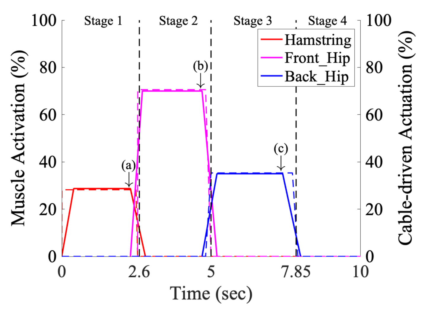
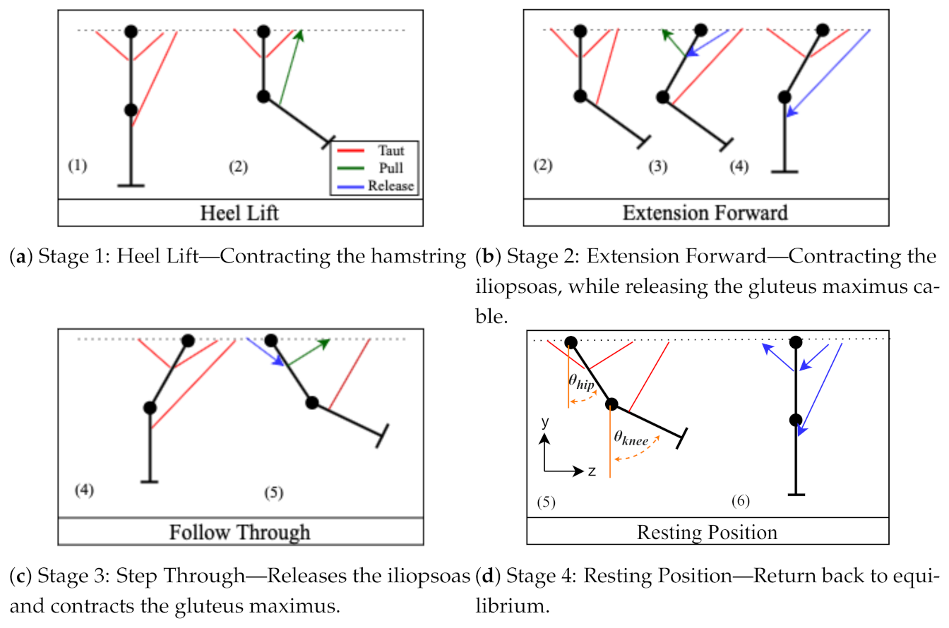
4. Control and Actuation Strategies

4.1. Open-Loop Control

One of the goals of the paper is to propose a pipeline, where a flexible manipulator will be modeled and fabricated to match the “desired kinematics” of a human leg. The approach is iterative, where the model and prototype inform each other and adapt to recapitulate the human leg geometry. Figure 4 shows an overview of the propose design strategy. We used the FD solver to provide the excitation pattern (Figure 5) that manipulates the hip and knee joints (Figure 6) throughout four the stages of gait in the sagittal plane shown in Figure 7. Stage 1: Heel Lift, starts from a neutral position, and contracts the hamstring-inspired cable to initiate knee flexion backward. Stage 2: Extension Forward, contracts the iliopsoas-inspired muscle causing the entire tensegrity structure to move forward, while the gluteus maximus-inspired and hamstring-inspired cables release the posterior hip and hamstring. Stage 3: Step Through, implements the combination of “leg-lift” and “swing”. When the iliopsoas flexes the lower limb at the hip, it drives the entire leg backward until it is positioned behind the body. Stage 4: Resting Position, restores the tensegrity structure to its neutral position. Once in the Resting Position, one cycle of gait has been completed, and if desired, the structure can continue the gait cycle repeatedly.
Modeling the tensegrity hip and knee joint in OpenSim 3.0 provided analysis on both passive and active connections for our physical prototype. Forces imported into the FD tool generate motions for each model. Each stage of gait excites one active element to contract at a time while the others remain passive or release tension. Each actuator in our physical model correlates with one of the three prominent active muscles in a human leg. The tangential force generated by the cable-driven actuators ( F T m a x ) during each stage of gait is computed as:
F T m a x = τ r
where r is the radius of the spool attachment for the motors, and τ is the stall-torque. Each cable-driven actuator contraction follows a sequential state machine.

4.2. Closed-Loop Control

The closed-loop control system follows the same procedure for imitating one cycle that was described in Section 4.1. The movement imitates the “virtual” muscle activation patterns (Figure 5) using three motors and two low-drift 9-axis BNO055 IMU (Inertial Measurement Unit equipped with an accelerometer, gyroscope, and magnetometer) sensors located at the base of the hip and knee (Figure 1).
Each sensor underwent a calibration process recommended by the manufacturer using a series of sensor-fusion algorithms that blends the accelerometer, magnetometer and gyroscope data into stable three-axis orientation output [40]. For calibrating the position of the sensors, we used the dynamics captured by the open-loop system along with the simulation to find the model’s limitations and available range of motion. This process executed a series of open-loop control motions for each stage of gait and used the motion capture recordings to correlate the angles of the compression elements with the IMU sensor readings. The sequential state machine requires a compensation for the forward kinematics and position. Here we monitor the hip ( θ h i p ) and knee ( θ k n e e ) angles using the IMU sensors and update their values in the state machine at each time iteration (see the “Control” panel of Figure 4). The actuation strategy relies on tracking the angles using the IMUs, applied forward kinematics using the motor driver, then updated the target angle ( θ r e f ) for the next stage of gait. This feedback loop incorporates a proportional controller that effectively manages the physical model to change the stages of gait once the system reaches a minimal steady-state error of 1.25% from the target position. In the event of an overshoot, the physical model is capable of correcting itself (Figure 4) when a gait stage has malfunctioned or is disturbed by an unanticipated outside force (i.e., pushing or pulling the structure out of the range of values).
To further validate our simulation, we compared its power consumption with the physical prototype’s (Figure 6C). The power consumption of the electrical motor is significantly larger than the other components. The microcontroller (290 mW) and sensors (25 mW) have a constant power requirement that was subtracted from the global power consumption to compute the power consumption of the motors. The model underestimates the idle power consumption, but it predicts well the power consumption during the third and forth stages of gait. The initial mismatch is most likely due to the differences between the ideal behavior of the OpenSim 3.0 muscles and commercial electrical motors at low speeds.

4.3. Gait Experiment

The goal of the gait experiment was to validate the OpenSim 3.0 model with the physical prototype and demonstrate the similarities of both of them with the human subject. A 3.5 (m) × 3.5 (m) × 3.5 (m) test area was instrumented with eight OptiTrack Prime 13 Watt infrared cameras that track retro-reflective markers at a frame rate of 60 Hz. The Motive post processing package was used to recorded the kinematic behavior of the robot and of a human volunteer performing a one-leg in-place gait motions. Marker’s positions were imported in OpenSim 3.0’s inverse kinematics (IK) package to compute the torques and angles (Figure 4), which were further imported in the forward dynamics (FD) tool to generated an actuation scheme (Figure 7) that manipulates each active element.

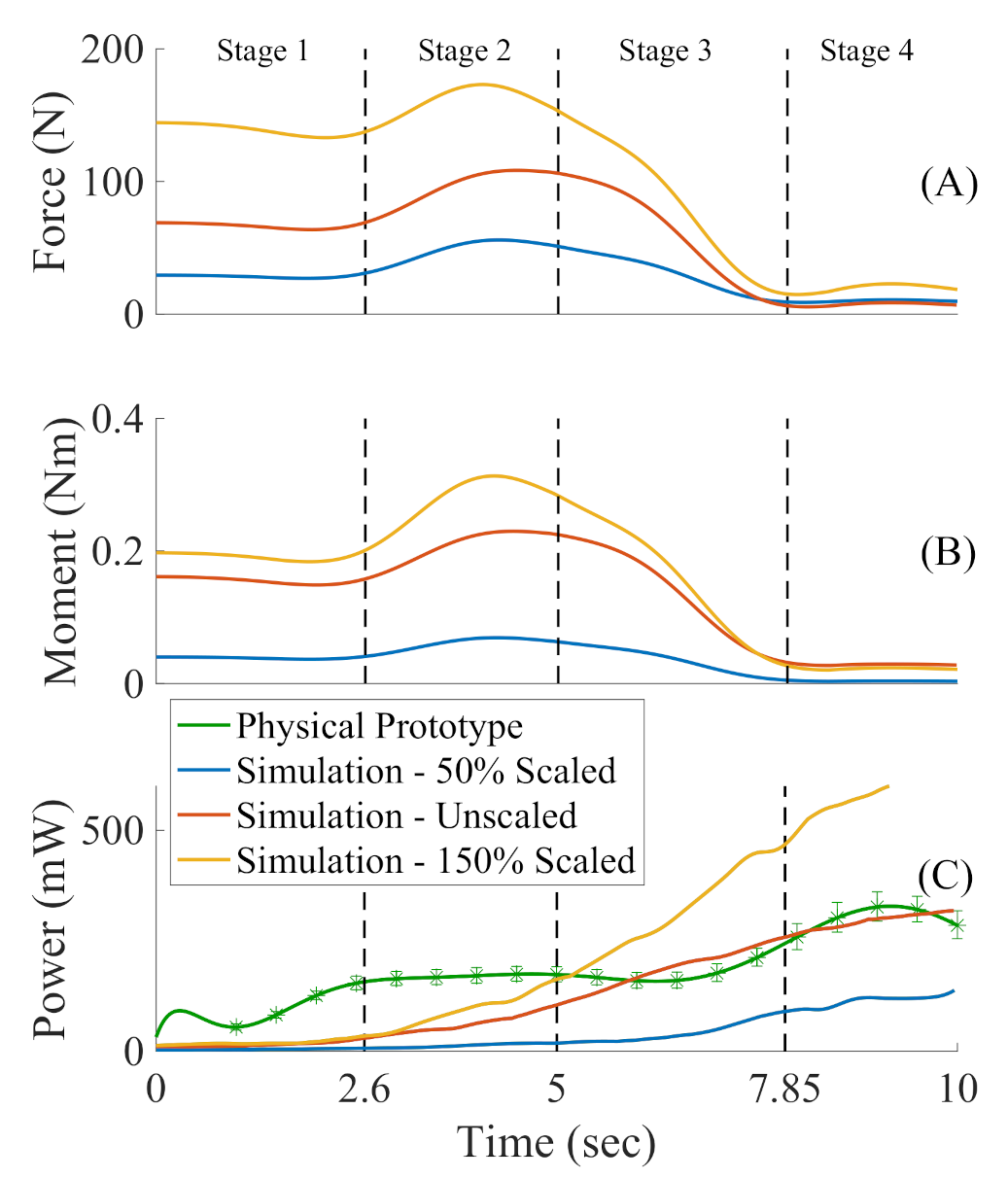
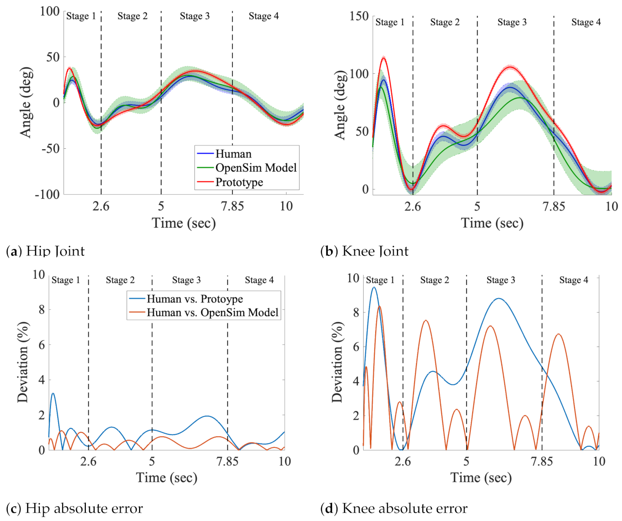
5. Results and Discussion

Most robotic structures that replicate the gait of human legs consist of rigid elements the are equivalent to biological bones, which are connected by revolute joints. The revolute joints act in a similar fashion to anatomically correct knee and hip joints; however, they have one main caveat: revolute joints have only one axis of rotation [8]. Anatomically inspired joints consist of rigid and flexible elements suspended in a network of muscles, tendons, and ligaments that work in unison to allow the joint to flex, move and contort [23,35]. The current work proposes an alternative approach: A design pipeline that develops flexible–rigid structures that recreate the kinematics of human legs.
Figure 8 shows the comparison between the hip and knee rotation angles during a full gait event. The OpenSim 3.0 prediction is shown in green, the flexible–rigid manipulator is shown in red and the human leg testing in blue. Figure 8a shows the hip rotation angles, and Figure 8c the knee rotation angles along the sagittal plane. The convention used here to define the rotation angles for the hip and for the knee is shown in Figure 7d—step 5. To compute the angles we associated a vector with the direction of each component of the manipulator ( V h i p and V k n e e ) and compute the angle between that component and the unit vector k associated with the z axes of the Cartesian coordinate system, which is assumed to be the resting position Figure 7a—step 1 and Figure 7d—step 6:
θ i = arccos ( V i · k | V i | | k | ) , i { h i p , k n e e }
All three systems demonstrated similar kinematics during the four stages of gait. Figure 8b show the absolute errors between the average measured and predicted hip angles and Figure 8d show the absolute errors between the average measured and predicted knee angles. The error between the human leg and the robotic prototype is shown in blue and the error between the human leg and the OpenSim 3.0 simulation is shown in red. It should be noted that the errors are very small. Due to the pelvic-inspired component suspended and confined to a mounted position, there is limited variance in the range of motion resulting in a lower absolute error compared to the knee. Both the kinematics of the femur-inspired element and the large angular displacement shown in each stage of gait (Figure 7) effect the absolute error of the knee (Figure 8d). Table 2 indicated that the movements for both Stage 1 and Stage 3 were both the most dramatic causing the largest error for both joints. The results between the OpenSim 3.0 model vs. Prototype and Human vs. Prototype show the accuracy of replicating the recorded motions with this system. Figure 9 tracks the trajectory of the end effector of the femur and tibia along the sagittal axis. The Cartesian coordinates ( v and u ) are computed using Equation (7) for each joint angle ( θ ) from the start and end of the gait experiment. This demonstrates the kinematic similarities of the human, simulation, and prototype gaits.

6. Conclusions

The proposed flexible–rigid design consists of three compression elements (“pelvis”, “femur”, and “tibia”) connected by two flexural joints (“hip” and “knee”). We simulated the human leg-inspired kinematic behavior of our proposed design within the OpenSim 3.0 simulation environment. The purpose of OpenSim 3.0 is to act as a human biomechanics solver, and we bridged and validated the ability to simulate custom musculoskeletal-inspired designs in the same environment.
The designs had a similar flexibility and range of motion to the human body for a specific gait-inspired experiment, as demonstrated by the kinematic results for joint angles (Figure 8). For the hip joint, the vectors stretch from the pelvic region to the bottom of the tibia element, and the knee’s range of motion used the lowest point of the femur to the tibia for the vectors. The structure was capable of extending the hip joint θ h i p flexion to approximately 40 , where human hip flexors are able to produce 35 across the sagittal plane throughout gait motions [41]. In the same plane, the knee joint, θ k n e e was capable of flexing to 110 , which is comparable to a human with 130 of knee flexion [41]. To further our kinematic analysis, we found the position of the end-effectors (Figure 9) to result in a maximum error of 3.3 % between the final positions of the simulations and the prototypes.
The behavior of the proposed manipulator was comparable to a human leg; however, this proof of concept was not intended to carry a load where future research could lead to a load-bearing self-standing flexible–rigid structure. The proposed methodology (Figure 4) for designing custom musculoskeletal-inspired models within the OpenSim 3.0 simulation environment demonstrated the potential for accurate kinematic and dynamic relationships between both human and assistive robotic devices.

Author Contributions

E.J.: project administration, writing, conceptualization; V.L.: visualization, data curation, resources, writing—review and editing; C.C.: software, validation, investigation, writing, visualization; N.C.: software, validation, simulation, formal analysis, data curation, visualization; M.L.N.: software, validation, investigation, formal analysis, visualization, writing; D.C.: electronics, design, validation, investigation; M.T.: supervision, project administration, writing—review and editing. All authors have read and agreed to the published version of the manuscript.

Funding

This research was supported by a grant made to the Braingeneers research group by Schmidt Family Futures. The funders had no role in study design, data collection and analysis, decision to publish, or preparation of the manuscript.

Institutional Review Board Statement

Under an UCSC IRB Protocol #HS3588, we have been able to collect motion captured data of a person.

Informed Consent Statement

We collected data on ourselves within this study, and the subject signed written informed consent as part of the UCSC IRB Protocol.

Data Availability Statement

Data availability will be given upon request to the corresponding author.

Acknowledgments

The authors would like to acknowledge the technical support of the Braingeneers research group as well as a donation made possible by Eric and Wendy Schmidt by recommendation of the Schmidt Futures program.

Conflicts of Interest

The authors declare no conflict of interest. The funders had no role in the design of the study; in the collection, analyses, or interpretation of data; in the writing of the manuscript, or in the decision to publish the results.

Abbreviations

The following abbreviations and symbols are used in this manuscript:
τ m net muscle moments
qgeneralized positions
amuscle activation values
lmuscle fiber lengths
Λ               muscle contraction dynamics
[ R ( q ) ] moment arms
Aactivation dynamics
xgeneralized terms for model controls
qvector of generalized positions
q ˙ vector for velocities
q ¨ vector for accelerations
[ M 1 ( q ) ] inverse of the mass matrix
τ vector of generalized forces
C ( q , q ˙ ) vector of Coriolis and centrifugal forces
G ( q ) vector of gravitational forces
F C E contractile elements
F P E parallel elements
F S E series elements
F P passive forces
F A active forces
l M normalized length of the unit muscle
l T normalized length of the unit tendon
F v normalized velocity of the unit muscle
α maximum pennation angle
nnumber of joints
μ moment
rradial distance
Qmuscle force
F T m a x controls the force applied
θ h i p hip joint angle
θ k n e e knee joint angle
θ r e f target angle
IMUinertial measurement unit
CADcomputer-aided design
3Dthree-dimensional

References

  1. Nashner, L. Adapting reflexes controlling the human posture. Exp. Brain Res. 1976, 26, 59–72. [Google Scholar] [CrossRef]
  2. Tur, J.M.M.; Juan, S.H. Tensegrity frameworks: Dynamic analysis review and open problems. Mech. Mach. Theory 2009, 44, 1–18. [Google Scholar]
  3. Scarr, G. Helical tensegrity as a structural mechanism in human anatomy. Int. J. Osteopath. Med. 2011, 14, 24–32. [Google Scholar] [CrossRef]
  4. Dwivedy, S.K.; Eberhard, P. Dynamic analysis of flexible manipulators, a literature review. Mech. Mach. Theory 2006, 41, 749–777. [Google Scholar] [CrossRef]
  5. Ozgoli, S.; Taghirad, H. A survey on the control of flexible joint robots. Asian J. Control 2006, 8, 332–344. [Google Scholar] [CrossRef]
  6. Hughes, J.; Culha, U.; Giardina, F.; Guenther, F.; Rosendo, A.; Iida, F. Soft manipulators and grippers: A review. Front. Robot. AI 2016, 3, 69. [Google Scholar] [CrossRef] [Green Version]
  7. George Thuruthel, T.; Ansari, Y.; Falotico, E.; Laschi, C. Control strategies for soft robotic manipulators: A survey. Soft Robot. 2018, 5, 149–163. [Google Scholar] [CrossRef] [PubMed]
  8. Zoss, A.B.; Kazerooni, H.; Chu, A. Biomechanical design of the Berkeley lower extremity exoskeleton (BLEEX). IEEE/ASME Trans. Mechatron. 2006, 11, 128–138. [Google Scholar] [CrossRef]
  9. Haegele, M.; Maufroy, C.; Kraus, W.; Siee, M.; Breuninger, J. Musculoskeletal robots and wearable devices on the basis of cable-driven actuators. In Soft Robotics; Springer: Berlin/Heidelberg, Germany, 2015; pp. 42–53. [Google Scholar]
  10. Asbeck, A.T.; De Rossi, S.M.; Holt, K.G.; Walsh, C.J. A biologically inspired soft exosuit for walking assistance. Int. J. Robot. Res. 2015, 34, 744–762. [Google Scholar] [CrossRef]
  11. Costa, N.; Caldwell, D.G. Control of a biomimetic “soft-actuated” 10dof lower body exoskeleton. In Proceedings of the First IEEE/RAS-EMBS International Conference on Biomedical Robotics and Biomechatronics (BioRob 2006), Pisa, Italy, 20–22 February 2006; pp. 495–501. [Google Scholar]
  12. Tolley, M.T.; Shepherd, R.F.; Mosadegh, B.; Galloway, K.C.; Wehner, M.; Karpelson, M.; Wood, R.J.; Whitesides, G.M. A resilient, untethered soft robot. Soft Robot. 2014, 1, 213–223. [Google Scholar] [CrossRef]
  13. Ansarieshlaghi, F.; Eberhard, P. Hybrid Force/Position Control of a Very Flexible Parallel Robot Manipulator in Contact with an Environment. ICINCO 2019, 2, 59–67. [Google Scholar]
  14. Jiang, M.; Zhou, Z.; Gravish, N. Flexoskeleton printing enables versatile fabrication of hybrid soft and rigid robots. Soft Robot. 2020, 7, 770–778. [Google Scholar] [CrossRef]
  15. Juan, S.H.; Tur, J.M.M. Tensegrity frameworks: Static analysis review. Mech. Mach. Theory 2008, 43, 859–881. [Google Scholar] [CrossRef] [Green Version]
  16. Wang, N.; Tytell, J.D.; Ingber, D.E. Mechanotransduction at a distance: Mechanically coupling the extracellular matrix with the nucleus. Nat. Rev. Mol. Cell Biol. 2009, 10, 75–82. [Google Scholar] [CrossRef]
  17. Bruce, J.; Sabelhaus, A.; Chen, Y.; Lu, D.; Morse, K.; Milam, S.; Caluwaerts, K.; Agogino, A.M.; SunSpiral, V. SUPERball: Exploring tensegrities for planetary probes. In Proceedings of the 12th International Symposium on Artificial Intelligence, Robotics and Automation in Space (i-SAIRAS), Montreal, QC, Canada, 17–19 June 2014. [Google Scholar]
  18. Chen, L.H.; Kim, K.; Tang, E.; Li, K.; House, R.; Zhu, E.L.; Fountain, K.; Agogino, A.M.; Agogino, A.; Sunspiral, V.; et al. Soft spherical tensegrity robot design using rod-centered actuation and control. J. Mech. Robot. 2017, 9, 025001. [Google Scholar] [CrossRef]
  19. Friesen, J.; Pogue, A.; Bewley, T.; de Oliveira, M.; Skelton, R.; Sunspiral, V. DuCTT: A tensegrity robot for exploring duct systems. In Proceedings of the 2014 IEEE International Conference on Robotics and Automation (ICRA), Hong Kong, China, 31 May–7 June 2014; pp. 4222–4228. [Google Scholar]
  20. Hustig-Schultz, D.; SunSpiral, V.; Teodorescu, M. Morphological design for controlled tensegrity quadruped locomotion. In Proceedings of the 2016 IEEE/RSJ International Conference on Intelligent Robots and Systems (IROS), Daejeon, Korea, 9–14 October 2016; pp. 4714–4719. [Google Scholar]
  21. Levin, S.M. The tensegrity-truss as a model for spine mechanics: Biotensegrity. J. Mech. Med. Biol. 2002, 2, 375–388. [Google Scholar] [CrossRef]
  22. Mirletz, B.T.; Quinn, R.D.; SunSpiral, V. Cpgs for adaptive control of spine-like tensegrity structures. In Proceedings of the 2015 International Conference on Robotics and Automation (ICRA2015) Workshop on Central Pattern Generators for Locomotion Control: Pros, Cons & Alternatives, Seattle, WA, USA, 26–30 May 2015. [Google Scholar]
  23. Lessard, S.; Castro, D.; Asper, W.; Chopra, S.D.; Baltaxe-Admony, L.B.; Teodorescu, M.; SunSpiral, V.; Agogino, A. A bio-inspired tensegrity manipulator with multi-DOF, structurally compliant joints. In Proceedings of the 2016 IEEE/RSJ International Conference on Intelligent Robots and Systems (IROS), Daejeon, Korea, 9–14 October 2016; pp. 5515–5520. [Google Scholar]
  24. Baltaxe-Admony, L.B.; Robbins, A.S.; Jung, E.A.; Lessard, S.; Teodorescu, M.; SunSpiral, V.; Agogino, A. Simulating the human shoulder through active tensegrity structures. In Proceedings of the ASME 2016 International Design Engineering Technical Conferences and Computers and Information in Engineering Conference, Charlotte, NC, USA, 21–24 August 2016; American Society of Mechanical Engineers: New York, NY, USA, 2016; p. V006T09A027. [Google Scholar]
  25. Castro, D. Modeling the Human Knee Using Tensegrity. Ph.D. Thesis, University of California, Santa Cruz, CA, USA, 2017. [Google Scholar]
  26. Jung, E.; Ly, V.; Cessna, N.; Ngo, M.L.; Castro, D.; SunSpiral, V.; Teodorescu, M. Bio-inspired Tensegrity Flexural Joints. In Proceedings of the 2018 IEEE International Conference on Robotics and Automation (ICRA), Brisbane, Australia, 21–25 May 2018; pp. 1–6. [Google Scholar]
  27. Scarr, G. A consideration of the elbow as a tensegrity structure. Int. J. Osteopath. Med. 2012, 15, 53–65. [Google Scholar] [CrossRef]
  28. Lessard, S.; Bruce, J.; Jung, E.; Teodorescu, M.; SunSpiral, V.; Agogino, A. A light-weight, multi-axis compliant tensegrity joint. arXiv 2015, arXiv:1510.07595. [Google Scholar]
  29. Caluwaerts, K.; Despraz, J.; Işçen, A.; Sabelhaus, A.P.; Bruce, J.; Schrauwen, B.; SunSpiral, V. Design and control of compliant tensegrity robots through simulation and hardware validation. J. R. Soc. Interface 2014, 11, 20140520. [Google Scholar] [CrossRef] [Green Version]
  30. BulletPhysicsEngine. 2013. Available online: http://www.bulletphysics.org/ (accessed on 23 September 2021).
  31. Goyal, R.; Chen, M.; Majji, M.; Skelton, R.E. MOTES: Modeling of Tensegrity Structures. J. Open Source Softw. 2019, 4, 1613. [Google Scholar] [CrossRef]
  32. Pajunen, K.; Johanns, P.; Pal, R.K.; Rimoli, J.J.; Daraio, C. Design and impact response of 3D-printable tensegrity-inspired structures. Mater. Des. 2019, 182, 107966. [Google Scholar] [CrossRef]
  33. Delp, S.L.; Anderson, F.C.; Arnold, A.S.; Loan, P.; Habib, A.; John, C.T.; Guendelman, E.; Thelen, D.G. OpenSim: Open-source software to create and analyze dynamic simulations of movement. IEEE Trans. Biomed. Eng. 2007, 54, 1940–1950. [Google Scholar] [CrossRef] [Green Version]
  34. Vivian, M.; Tagliapietra, L.; Sartori, M.; Reggiani, M. Dynamic simulation of robotic devices using the biomechanical simulator OpenSim. In Intelligent Autonomous Systems 13; Springer: Cham, Switzerland, 2016; pp. 1639–1651. [Google Scholar]
  35. Wang, A.; Lu, J.; Ge, Y.; Yu, J.; Zhang, S. Simulation of Limb Rehabilitation Robot Based on OpenSim. In International Conference on Bio-Inspired Computing: Theories and Applications; Springer: Singapore, 2019; pp. 647–654. [Google Scholar]
  36. Kutilek, P.; Svoboda, Z.; Smrcka, P. Evaluation of bilateral asymmetry of the muscular forces using opensim software and bilateral cyclograms. In Mechatronics 2013; Springer: Cham, Switzerland, 2014; pp. 801–808. [Google Scholar]
  37. Scarton, A.; Jonkers, I.; Guiotto, A.; Spolaor, F.; Guarneri, G.; Avogaro, A.; Cobelli, C.; Sawacha, Z. Comparison of lower limb muscle strength between diabetic neuropathic and healthy subjects using OpenSim. Gait Posture 2017, 58, 194–200. [Google Scholar] [CrossRef] [PubMed]
  38. SimTK. How Forward Dynamics Works. 1993. Available online: https://simtk-confluence.stanford.edu/display/OpenSim/How+Forward+Dynamics+Works (accessed on 25 August 2017).
  39. Thelen, D.G. Adjustment of muscle mechanics model parameters to simulate dynamic contractions in older adults. J. Biomech. Eng. 2003, 125, 70–77. [Google Scholar] [CrossRef] [PubMed] [Green Version]
  40. Adafruit Unified BNO055 Driver (AHRS/Orientation). Available online: https://github.com/adafruit/Adafruit_BNO055 (accessed on 10 March 2021).
  41. Appleton, B. Stretching and Flexibility: Normal Ranges of Joint Motion. 2007. Available online: https://people.bath.ac.uk/masrjb/Stretch/stretching_8.html (accessed on 20 August 2017).
Figure 1. The proposed system, consisting of three compression elements (“Tibia”,“Femur” and “Pelvis”) and two flexural joints (“Knee” and “Hip”) controlled by three active tensile elements.
Applsci 11 09351 g001
Figure 2. Tensegrity Flexural Joint: Hip.
Applsci 11 09351 g002
Figure 3. Tensegrity Flexural Joint: Knee.
Applsci 11 09351 g003
Figure 4. Flowchart illustrating the design process.
Applsci 11 09351 g004
Figure 5. The applied activations by the three virtual “muscles” in the OpenSim 3.0 simulation environment (full line), and the intensity from the cable-driven actuators on the prototype (dotted lines). The varying levels of actuation (i.e., applied forces) input into the simulated models generalize an approximation for how to actuate the muscle-inspired cables in the prototype. Labels (a–c) indicate where the applied contracting muscles release.
Applsci 11 09351 g005
Figure 6. (A) Applied forces from all the active elements on the simulated model at varying sizes (50%, 100%, and 150% scales) show that a smaller model requires similar amounts of forces to replicate the four stages of gait. (B) Simulated moments (N·m) on the hip joint throughout the four stages of gait estimate the required actuators. (C) Power consumption (mW) of the structure is similar to the simulation and the physical prototype performing the four stages of gait. The average of the few trials (solid green line) for the physical prototype created the upper and lower error bars. As we enlarge the model size, the forces necessary to produce the same motion increase. Increasing the size of the simulated models demonstrated a significant spike in overall energy consumption. It is worth noting that the 100% scaled simulation model is the same size as the physical prototype.
Applsci 11 09351 g006
Figure 7. Outline of the active elements during the four stages of gait. Each pull (green) activates the cable-driven actuator to contract and shorten the muscle. The release of muscles (blue) reverses the direction of the actuator. In (Stage 4) the orange shows how the angles for the hip and knee were tracked.
Applsci 11 09351 g007
Figure 8. Simulated and measured angles of the hip (a) and knee (b) joints during the four stages of gait, and (c,d) the absolute errors, between angles across multiple trials (see Table 2). The shaded range represents the lower and upper limits of motion through simulated trials with the chosen configuration in a solid line.
Applsci 11 09351 g008
Figure 9. The bottom retro–reflective markers on the human and prototype are the motion–tracked end–effectors. Both end–effectors demonstrate similar behavior, validating the kinematics of the proposed design. During the gait motion, ‘o’ is the start, and the ‘*’ is the end.
Applsci 11 09351 g009
Table 1. Muscle element specific parameters used for simulation.
Muscle Element F 0 M (N) L 0 M (m) L s T α M (deg)
Active1000.1281.8<1
Thelen [39]14000.0902.47
F 0 M maximum isometric force; L 0 M optimal fiber length; L s T max tendon slack length in relation to muscle length; α M muscle fiber pennation angle.
Table 2. Maximum absolute error (%) for each stage of gait.
Human vs. Prototype JointStage 1Stage 2Stage 3Stage 4
Hip3.11.31.90.97
Knee9.44.58.84.7
Human vs. OpenSim 3.0 ModelStage 1Stage 2Stage 3Stage 4
Hip vs. Prototype Joint1.030.540.750.41
Knee vs. Prototype Joint8.37.57.26.7
Publisher’s Note: MDPI stays neutral with regard to jurisdictional claims in published maps and institutional affiliations.

