Modal Analysis of the Lysozyme Protein Considering All-Atom and Coarse-Grained Finite Element Models

Abstract

Proteins are the fundamental entities of several organic activities. They are essential for a broad range of tasks in a way that their shapes and folding processes are crucial to achieving proper biological functions. Low-frequency modes, generally associated with collective movements at terahertz (THz) and sub-terahertz frequencies, have been appointed as critical for the conformational processes of many proteins. Dynamic simulations, such as molecular dynamics, are vastly applied by biochemical researchers in this field. However, in the last years, proposals that define the protein as a simplified elastic macrostructure have shown appealing results when dealing with this type of problem. In this context, modal analysis based on different modelization techniques, i.e., considering both an all-atom (AA) and coarse-grained (CG) representation, is proposed to analyze the hen egg-white lysozyme. This work presents new considerations and conclusions compared to previous analyses. Experimental values for the B-factor, considering all the heavy atoms or only one representative point per amino acid, are used to evaluate the validity of the numerical solutions. In general terms, this comparison allows the assessment of the regional flexibility of the protein. Besides, the low computational requirements make this approach a quick method to extract the protein’s dynamic properties under scrutiny.

1. Introduction

Most of the known biological functions are only conceivable because of the wide range of operations performed by proteins [1,2]. The folding and unfolding process is one of these aspects that must be understood to comprehend how these macromolecules operate at the nanometer scale. The protein conformational states are not static and they depend on many factors, such as the surrounding environment and temperature [3]. The study of the three-dimensional protein structure is rather complex, allowing many different approaches to the problem. The application of coarse-grained systems usually enables the analysis of larger proteins composed of several hundred amino acids with relatively low computational effort, typically providing global descriptions [4]. For specific problems, the atomically-detailed models can, to some extent, contribute to further and more accurate information [5]. To this purpose, molecular dynamics (MD) dives deeper into higher accuracy evaluation of the actual phenomena in place. However, its high computational burden often prevents its applicability in studying the large-scale slow motions of the protein, which are known to be correlated with the biological function.

In the last decades, it was shown that simplified calculations based on the assumption of a harmonic potential can provide accurate insights into protein dynamics. Normal mode analysis (NMA) was developed for this purpose as a simplified yet powerful tool to extract the functional modes of the protein structure. Levitt et al. showed that NMA with internal coordinates is particularly suited for modeling the collective motions, enabling the visualization of biologically relevant modes, and it is complementary to the more time-consuming MD simulations [6]. However, these NMA calculations still relied on a detailed knowledge of the complex semi-empirical potentials that characterize the interactions amongst all the atoms of the system. Afterward, it was shown by Tirion that a simplified single-parameter harmonic potential is good enough to reproduce the slow dynamics of the protein correctly while avoiding the expensive and sometimes inaccurate NMA energy minimization of the reference structure [7]. Subsequently, it was recognized that even coarse-grained representations of the protein, only based on the position of the C^α atoms of the crystal structure, lead to useful predictions of the slow protein dynamics as well as the observed fluctuations [8,9,10]. These models are known as the Elastic Network Models (ENMs), and various developments have been carried out in the following years by various research groups [11,12,13,14,15,16,17]. The great amount of work in ENM development was because, despite their inherent simplification, these structural models were found to provide impressive insights on the biological mechanisms and flexibility of the protein [18,19,20,21,22,23,24,25,26,27,28].

It is astonishing that such simplified models, purely based on Structural Mechanics concepts, allow us to understand protein motions and biological activity, which are very complex in nature. The present work encompasses the protein’s representation as a simple truss-like domain, similar to macroscale structures in the field of civil engineering, using a finite element (FE) approach. The protein’s dynamic properties are extracted by carrying out the modal analysis of the system and considering different initial assumptions. Then, the results of the calculations are compared to experimental data and the outcomes of other numerical studies. Many authors have indicated that underdamped frequencies describing collective modes at GHz and THz frequencies may be relevant to the biochemical function [29,30,31,32,33,34,35]. The hen egg-white lysozyme is the chosen protein for this study due to the extensive bibliography and experimental results related to it. This protein has an essential role in breaking bacterial cell walls and can be found in human milk and tears. The geometric description of the crystallized form can be found in the Protein Data Bank (PDB code: 4YM8) [36] and consists of 129 amino acids and approximately 1000 heavy atoms.

Experimental approaches have also been widely applied to extract the dynamic properties of the lysozyme. THz time-domain spectroscopy (TDS) is one of the capable tools, providing information regarding inter-molecular and intra-molecular motions of crystalline materials at THz frequencies [29]. However, water absorption has a massive influence on the results. Various authors have also considered the application of Raman spectroscopy, developed explicitly to capture information at frequencies below 1 THz and with the low influence of the liquid levels [32,33,35,37,38,39]. This type of ultra-low vibrational spectroscopy technique collects information about the protein motions through the phenomenon of inelastic scattering of the incident light. The formed Raman plot results from the difference in intensity between the incident light and the scattered photons for a given sample [40,41,42,43]. The necessity to collect low frequencies comes in place due to studies pointing to the biological functions and protein activation at those levels. Raman spectroscopy measurement for the lysozyme was carried out by Carpinteri et al. [32]. The data collected from the samples showed peaks close to the region of 0.84 THz, which were assumed to be associated with global expansion/contraction vibrational modes. The other extracted peaks lying in the range between 24 and 50 THz were found to be related to specific amino acid groups [32].

This work focuses on the numerical evaluation of the lysozyme vibrations, where the selected protein was modeled as an all-atom and coarse-grained truss-like structure. A FE code was developed in MATLAB, extracting the dynamic properties through modal analysis. For visualization purposes, the ANSYS APDL and Chimera software were applied to display clear views of the results.

2. Methodology

A basic introduction about modal analysis and the conditions of constructing a FE truss-like structure is carried out in this section. The reader can find here detailed information about all the simplifications and assumptions of the models, which are crucial for a correct interpretation of the results.

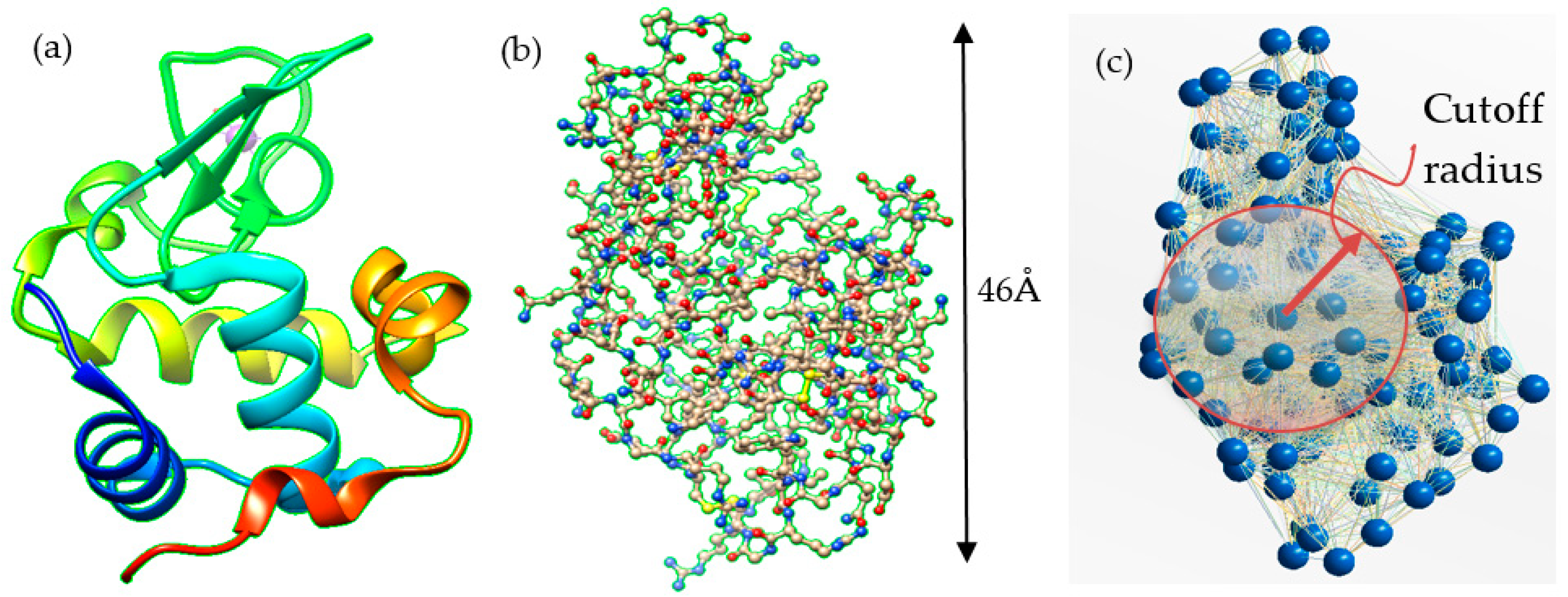
2.1. The Truss-Like Structure, the Connectivity Assumption and Modal Analysis

This work focuses on the all-atom and coarse-grained elastic schemes for the protein structure. The assumptions are the same for both cases, with small variants between them. The all-atom model considers each heavy atom as the node of the truss, whereas the coarse-grained takes one point for each amino acid (residue) as a point mass. In the real structure of proteins, peptide bonds connect various amino acids in different patterns, forming secondary structures like α-helices and β-sheets. Figure 1a displays the tertiary structure of the lysozyme, describing the closely packed domain. However, these structures are not taken into account directly for the generation of the numerical models.

The criterion of geometrical proximity generates the connections between the nodes, i.e., a cutoff value sets a spherical horizon from every designated node. In Figure 1c, the sphere of influence is shown graphically. Links are created from the central node connecting it to the surrounding ones lying below the selected cutoff value. The connections are defined as massless elements, having only axial stiffness k_ij and no bending, shear, or torsional rigidity. In this type of analysis, only the axial rigidity E_ijA_ij, which is defined by the Young’s Elastic Modulus E_ij and cross-sectional area A_ij, is essential [44]. The 3D representation of the 6 × 6 stiffness matrix of the elastic element connecting nodes i and j is shown in Equation (1), where x, y, and z are the global coordinates of the node in the 3D space, and L_ij the length of the elastic connection.

$$\begin{array}{c}{k}_{ij}=\frac{E_{ij}{A}_{ij}}{L_{ij}}\left[\begin{array}{cccccc}{C}_x^2& C_x{C}_y& C_x{C}_z& -C_x^2& -C_x{C}_y& -C_x{C}_z\\ C_x{C}_y& C_y^2& C_y{C}_z& -C_x{C}_y& -C_y^2& -C_y{C}_z\\ C_x{C}_z& C_y{C}_z& C_z^2& -C_x{C}_z& -C_y{C}_z& -C_z^2\\ -C_x^2& -C_x{C}_y& -C_x{C}_z& C_x^2& C_x{C}_y& C_x{C}_z\\ -C_x{C}_y& -C_y^2& -C_y{C}_z& C_x{C}_y& C_y^2& C_y{C}_z\\ -C_x{C}_z& -C_y{C}_z& -C_z^2& C_x{C}_z& C_y{C}_z& C_z^2\end{array}\right]\\ C_x=\frac{x_j-x_i}{L_{ij}},C_y=\frac{y_j-y_i}{L_{ij}},C_z=\frac{z_j-z_i}{L_{ij}}\end{array}$$

(1)

It has to be noted that both in the all-atom and coarse-grained model used in this work, a unique value of the axial rigidity EA has been set for all the elastic connections, consistently with some previous works [15,32,34], i.e., E_ijA_ij = EA. In this way, the axial stiffness of each connection k_ij turns out to be inversely proportional to the length of the connection itself L_ij. The definition of nodal locations is discussed in the next section, depending on the considered model (all-atom or coarse-grained).

The masses are concentrated at the nodes; therefore, the lumped mass assumption can be set, originating diagonal mass matrices and facilitating the numerical solution. The all-atom model uses the atomic mass of each atom at the specific position as provided in the PDB file (PDB code: 4YM8) [36]. On the other hand, for the coarse-grained structure scheme, the amino acid masses are condensed in a single representative point.

A linear elastic structure assumes a direct superposition process to obtain the global stiffness K and mass M matrix. The multi-degree of freedom (MDOF) system, in our case, is addressed as a free MDOF structure where no damping ζ is considered in the equations of motion. The solution for Equation (2) involves sinusoidal displacement functions, where the amplitude vector a and frequency vector ω are associated with each DOF. The non-trivial solution only is achieved when the determinant of Equation (3) is equal to zero, leading to the characteristic free-vibration equation. For a system counting N nodes in the three-dimensional space, the problem is characterized by 3N DOFs. The extraction of 3N eigenvectors and 3N eigenvalues allows us to obtain the undamped mode shapes and natural frequencies, respectively [45].

$$\mathit{M}\ddot{u}\left(t\right)+\mathit{K}u\left(t\right)=0 \to \left(-{\omega }^2\mathit{M}+\mathit{K}\right)a sin\left(\omega t+\theta \right)=0$$

(2)

$$\left(-{\omega }^2\mathit{M}+\mathit{K}\right) a=0 \therefore \det \left[-{\omega }^2\mathit{M}+\mathit{K}\right]=0$$

(3)

Since there are no external boundary restrictions defined for the structure, i.e., the protein is not externally constrained, the first six eigenvalues/eigenvectors of the solution are discarded. As a matter of fact, these are just due to the rigid translational and rotational modes caused by the lack of any external restriction and, consequently, the corresponding modes are just free-body vibrations at zero frequency.

2.2. Definitions about the All-Atom Model

Figure 1b presents the all-atom 3D model of the lysozyme with atomic positions. All the 1000 heavy atoms, i.e., carbon, nitrogen, oxygen, and sulfur atoms, are displayed. In this case, the hydrogen atoms are disregarded due to their low mass participation. The largest longitudinal dimension of lysozyme is also shown in the figure, which corresponds to 46 Å, i.e., 4.6 nm. The connections shown in Figure 1b, taken from the Chimera software, display the covalent bonds among the protein’s heavy atoms. Carpinteri et al. developed a frame-like model of the lysozyme using only the covalent bonds, as presented in Figure 1b, with a frame structure with extremely high flexural and polar momenta of inertia, in order to evaluate the expansion/contraction vibrations in the THz range [32]. Nevertheless, these connections are not the only ones used in this study. In fact, applying an equivalent truss-like description with such short-range connections is not possible due to the resulting lack of rigidity of the overall system. Spheres of influence (cutoffs) are generated using truss elements with 4, 6, 8, 10, 12, 15, 20, 25, and 30 Å. Consequently, 2994 modes (3 × 1000 − 6) can be extracted from each truss-like configuration for further investigation.

2.3. Definitions about the Coarse-Grained Model

Figure 1c shows an example of the lysozyme structure with 129 nodes interconnected. Each node corresponds to a representative point of each amino acid. The applied cutoffs are the same used in the work of Scaramozzino et al. [15], i.e., 8, 10, 12, 15, and 20 Å. However, contrary to this previous work, the nodal masses are not averaged with a constant value for all residues. Conversely, the actual mass of each amino acid is set according to its actual constituents, i.e., all the atomic masses are compressed at the representative node. This approach generates an averaged mass of around 18.48 × 10⁻²⁶ kg, with a standard deviation of 5.4 × 10⁻²⁶ kg throughout the protein structure. A total of 381 modes (3 × 129 − 6) are then extracted in these circumstances from each truss-like coarse-grained configuration.

Traditionally, the coarse-grained representations of the protein structure define the residues located at the C^α atoms, which lie on the protein backbone [9,10,15]. In this analysis, we take a different approach; namely, the representative position of each amino acid is located at its center of mass (CM), which is typically the assumption taken in macroscopic structures. The proposal came after observing that, within the distribution of the B-factors, the C^α atom is rarely the node with the highest fluctuation (see below). As a matter of fact, it is reasonable that the highest fluctuations should be biased towards the external side chains, especially for the larger amino acids, due to the increased flexibility of the side chains compared to backbone atoms. Operatively, the CM of each amino acid’s position is simply calculated based on the mass-weighted average locations of all constituent atoms. The positions of the CMs are then used to build the truss-like coarse-grained model and ultimately extract the dynamic properties of the protein.

2.4. The Experimental Debye-Waller Factors or B-Factors

Numerical results from dynamic calculations are commonly compared with experimental data used in organic chemistry and correlated fields. The B-factor, also called the temperature factor or Debye-Waller parameter, is one of the main research lines when dealing with proteins and their flexibility. It is influenced by the dynamic disorder caused by the temperature and the static disorder [46]. Equation (4) shows the most widespread form for this factor, where a is the mean displacement caused by thermal motion extracted by crystallography attenuation of X-ray or neutron scattering. It basically represents the displacement variation from the equilibrium position of a given atom [47].

$$B=\frac{8 {\pi }^2}{3}\langle a^2\rangle$$

(4)

The researchers use the Debye-Waller factor for a wide range of different purposes. Some of them use the Debye-Waller factor to infer the flexibility of atoms, chains, or regions. Many studies initially considered only the B-factor of the C^α atoms, as these are usually associated with the most representative atom of the amino acid within the protein backbone [48,49,50]. However, nowadays, the temperature factor is found in the PDB file for all atoms for every single static configuration of the protein. It must be pointed out that the provided X-ray data accuracy is not better than 10% [47] and the collected results must be used with care [51,52,53]. The resolution is one of the parameters that has a significant effect on the experimental results. Scholars have also indicated that highly flexible regions, having B-factors generally higher than the other areas of the protein, can behave like hinges that drive the motion associated with the protein conformational change [54].

The B-factor can be theoretically computed using the results derived from the dynamic analysis by applying a direct summation of the eigenvectors. Equation (4) is adapted into Equation (5) and used in this work to calculate the B-factors arising from the normal modes, as reported in [15,55]. The computed B-factor for every node i is the result of the summation of the 3N − 6 non-rigid mass-weighted modes n. The sum can be truncated for values lower than 3N − 6, usually decreasing the necessity to add higher frequencies, as B_i grows according to the inverse square of the angular frequency ω_n. The term k_b in Equation (5) indicates the Boltzmann constant (~1.38 × 10⁻²³ J/K) and T is the absolute temperature in Kelvin.

$$B_i=\frac{8 {\pi }^2}{3}{k}_{b}T{\displaystyle \sum }_{n=7}^{3N}\frac{{\left(a_{ix}^2+a_{iy}^2+a_{iz}^2\right)}_n}{{\omega }_n^2}$$

(5)

Alongside the fact that the goal is to compare segments of the same protein, a better form to analyze the local flexibility is through the normalized B-factor (B′). This is defined via Equation (6), where σ is the standard deviation and μ is the average value of the B-factors profile.

$${B^{\prime }}_i=\frac{B_i-\mu \left(B\right)}{\sigma \left(B\right)}$$

(6)

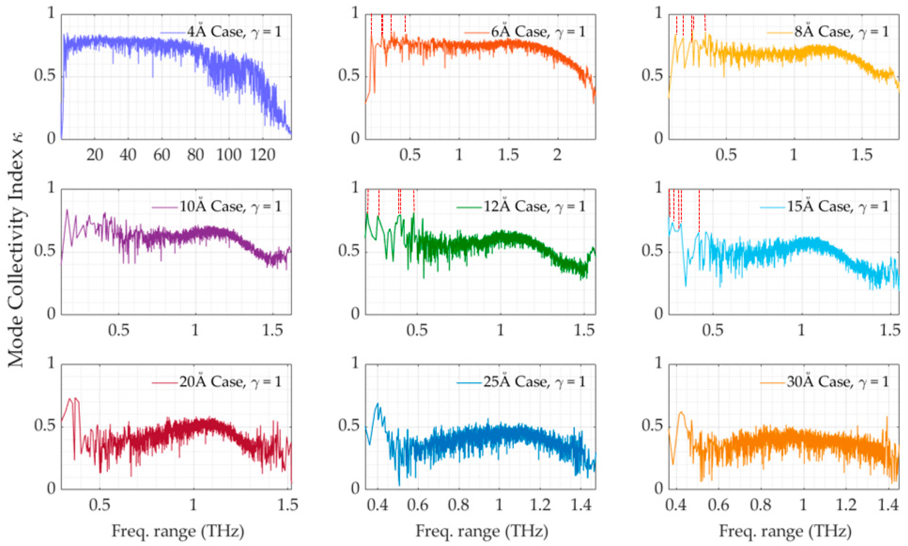
2.5. Collectivity of the Protein Motions

The modal analysis provides a lot of information about the structural motion, but plenty of data needs to be interpreted according to the desired goal. In the case of protein dynamics, and specifically for an equivalent truss-like structure, the main interest is to find collective motions. The motion of only one or a few fragments usually does not provide insights about the structure’s slow dynamics, which is the one more related to biological behavior. For this reason, we are mainly interested in concerted motions that involve major parts of the protein. The mode collectivity index κ [18,56] has been regarded as an adequate tool for this purpose. In this study, the index generates a value, between 1/N and 1 (N being the number of nodes), for each mode n based on the degree of the collectivity of the investigated motion.

The eigenvector associated with the mode n is transformed into a vector with the absolute displacements of the N nodes. The displacement components d_ni must be normalized in a p_ni form following Equation (7). The mode collectivity index κ can then be calculated according to Equation (8), where κ_n will vary from 1/N up to 1. Higher collectivity indexes can conventionally be associated with more global motions, while smaller ones are commonly related to more localized movements. The exponent γ permits to amplify signals for larger components of p_ni. In this analysis, γ is kept as a unitary value.

$$p_{ni}=\frac{{\left|d_{ni}\right|}^Y}{{{\displaystyle \sum }}_{s=1}^N{\left|d_{ns}\right|}^{\gamma } } , {\displaystyle \sum }_{i=1}^N{p}_{ni}=1$$

(7)

$${\kappa }_n=\frac{1}{N}\exp ({\displaystyle \sum }_{i=1}^N\left[p_{ni}\ln \left(p_{ni}\right)\right])$$

(8)

The analysis of the collectivity index throughout the extracted modes can indicate the most collective motions and therefore, identify the potential modes relevant to the biological mechanism. This can be obtained for each considered cutoff value, and structure representation (all-atom or coarse-grained), allowing us to compare the different cases.

2.6. The Scaling Procedure

The protein analysis typically deals with orders of magnitude of 10⁻²⁶ kg for the masses (Da), 10⁻¹⁰ m for the distances (Å), and 10¹² Hz for the frequencies (THz). An exemplification given with simple vibrational analysis is provided by Carpinteri et al. [32], demonstrating how these values are established for large proteins and chemical groups. While performing the numerical calculations with such orders of magnitudes, the results could be affected in terms of precision when using such very low and high numbers. Therefore, a scaling procedure should be implemented to avoid possible numerical problems. Extensive details about the adopted scaling procedure can be found in Carpinteri et al. [32,34].

3. Results and Discussion

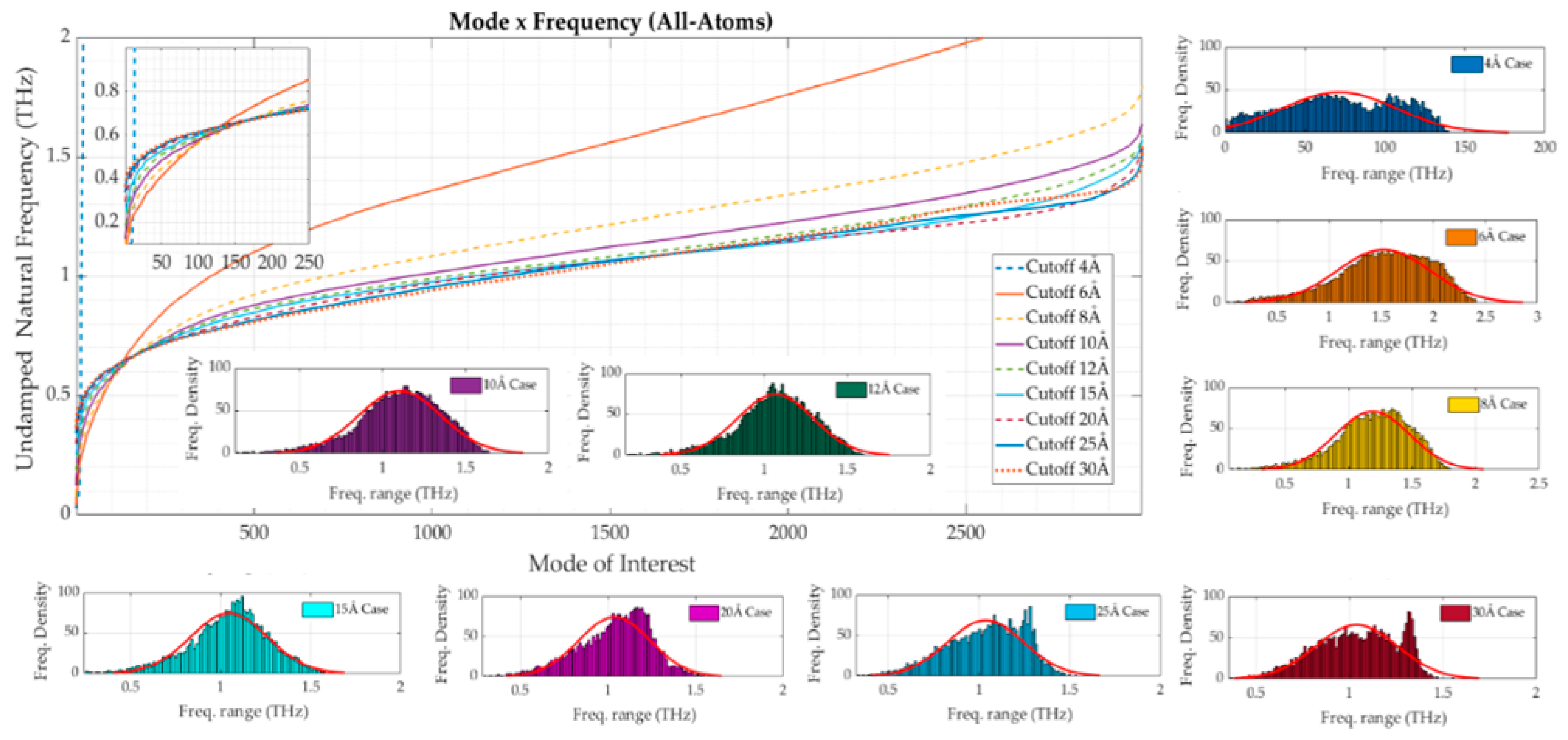
3.1. All-Atom Model

The 1000 heavy atoms of the lysozyme have their temperature factors (B-factors) available in the PDB file. These experimental values were used as the reference benchmark to fix the value of the adopted axial rigidity EA. This procedure was performed to establish a quantitative comparison between the calculated and experimental values of the B-factors. Note that the resulting axial rigidity EA does not necessarily have a physical meaning since it only represents the mean rigidity of all the elastic connections simulating the complex chemo-physical interactions among the atoms. Although shorter links can be associated with covalent bonds, the longer ones are related to weaker interactions due to electrostatic and Van der Waals effects. These are not easily quantifiable with the use of a single-parameter harmonic potential; therefore, the value of the axial rigidity set here is only understood as the average strength of the generated elastic connections.

Nevertheless, the choice of the EA value has a certain influence on the obtained vibrational frequencies. Moreover, choosing the value of the axial rigidity to have consistency between the mean values of the numerical and experimental B-factors leads to some consequences in the relationships between the different cutoffs.

Table 1. The defined axial rigidity and stiffness for each case regarding the all-atom models. The axial rigidity was selected to match the mean B-factor extracted experimentally for all heavy atoms.

Cutoff (Å)	Axial Rigidity EA (N)	Nº of Connections	Average Stiffness k (N/m)
4	3471.7 × 10−10	5979	1.36 × 103
6	0.6470 × 10−10	19,151	0.1675
8	0.2436 × 10−10	39,456	0.0485
10	0.1462 × 10−10	69,143	0.0236
12	0.1046 × 10−10	106,767	0.0143
15	0.0739 × 10−10	175,875	0.0083
20	0.0527 × 10−10	301,919	0.0047
25	0.0450 × 10−10	408,088	0.0035
30	0.0424 × 10−10	46,6426	0.0031

shows the obtained axial rigidity and average stiffness for the considered cutoff values concerning the all-atom models. These values demonstrate that the mean rigidity decreases as the number of connections increases. Therefore, increasing the network’s connectivity leads to the necessity of considering weaker elastic connections to have the same average thermal fluctuations.

As shown in Table 1, the model with a cutoff value of 4 Å presents a very low number of connections with respect to the other cases, which can generate some problems considering uniaxial elements. For this reason, this model is found to require a very high value of axial rigidity (~1360 N/m) due to the low number of generated connections. Such configuration is not tied enough to allow a suitable truss structure. On the other side, the model with a cutoff value of 30 Å constitutes more than half of the maximum body length (46 Å) and it creates a massive number of connections. However, the axial stiffness is proportional to the inverse of the connection length, making most of the longer links less critical for larger cutoffs.

The results from the analysis involving the B-factors for all heavy atoms are displayed in Figure 2. Three sets of plots are arranged to facilitate the visualization. In Figure 2a, the normalized B-factors arising from the lower cutoffs, i.e., 4, 6, and 8 Å, are shown. Figure 2b shows the ones with the medium cutoff values, i.e., 10, 12, and 15 Å. In Figure 2c, the ones with the higher cutoffs, i.e., 20, 25, and 30 Å. The vertical lines reported in each graph indicate the location of the 129 C^α atoms along the sequence of all heavy atoms. It was observed that the B-factors at the C^α locations do not necessarily reach their highest value for the considered amino acid. As briefly remarked in Section 2.3, this interesting feature led us to address a change in the node position for the construction of the coarse-grained model (see Section 3.2) and consider the CM of the amino acid as the representative node.

By observing Figure 2a, it is evident that the curve related to the model with the cutoff of 4 Å presents exceptionally high peaks in four positions. This effect occurs because these protein regions are too loose due to the very short-range connections, leading to tremendously localized flexibility. This massive deviation causes the necessity to apply the high rigidity value cited in Table 1 to match the average value of the experimental B-factors. Therefore, the application of such a small cutoff value is clearly not adequate for the proposed technique and the investigated protein, thus demanding larger spheres of influence.

The 6 Å and 8 Å cases are capable of providing more information about global and localized flexibility. Most of the peaks in the computed profile of numerical B-factors exhibit some similarity with the experimental ones. The remaining cutoff values, i.e., 10, 12, 15, 20, 25, and 30 Å, present very similar profiles, matching pretty well with the experimental B-factors. However, the amplitude of flexibility in some regions changes to some extent depending on the specific case, i.e., the specific cutoff value. As can be appreciated by comparing Figure 2a–c, the augment of the sphere of influence adds more details to the B-factors curves. Some of these increments are subtle, but they can contribute to the changes in the shape of the profile. These modifications can also highlight minor peaks not captured with other selected cutoffs.

Three sections are also amplified in the lower panel of Figure 2 for better visualization: atoms 50–250, 350–600, and 750–1000. Overall, it can be noted that the trends provided by the numerical solutions meet fairly accurately with the experimental one. Some specific observations are cited:

○

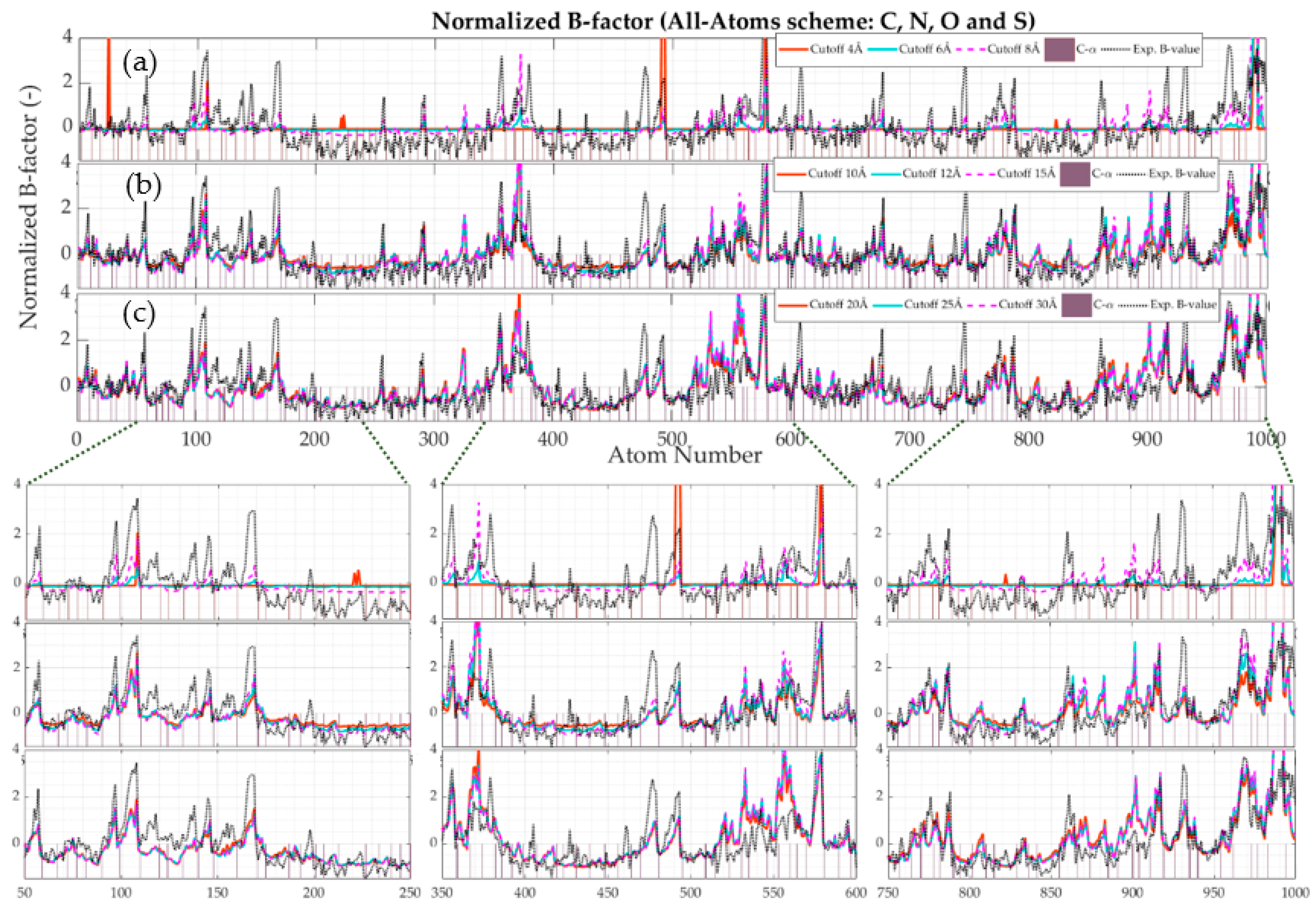
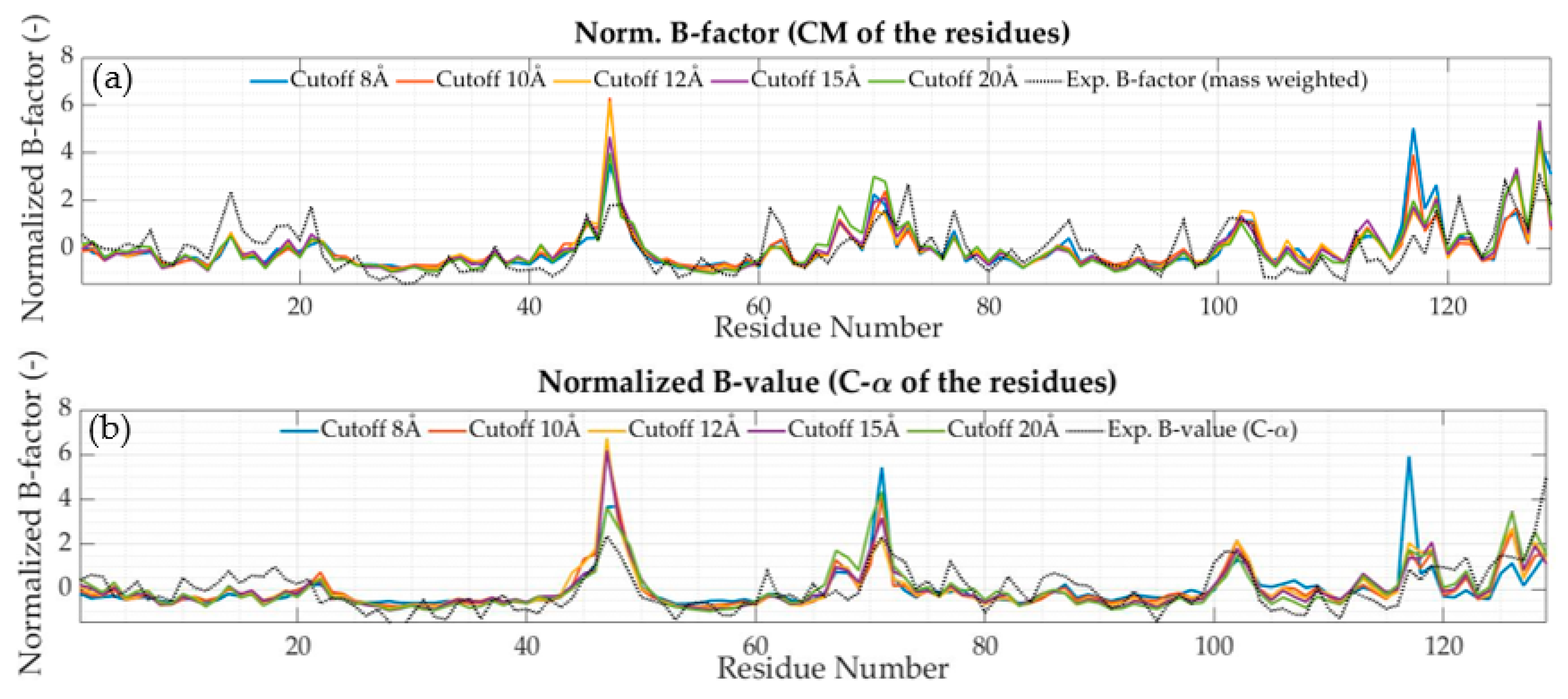
in the region 50–250, the major experimental peaks agree with the numerical ones from the model with a cutoff value of 10 Å onwards. For small fluctuations, it is hard to confirm a good representative relationship between the solutions;

○

in the region 350–600, node 379 shows a high experimental B-factor, but none of the numerical solutions provides such increased flexibility. The models are not able to capture this particular behavior. This can either be due to deficiencies in the simplified truss models or measurement errors in the experimental B-factors. Some other smaller peaks have similar patterns. At node 478, the effect that arises from increasing the cutoff value is clearly seen;

○

in the region 750–1000, nodes 991 and 992 present a substantial peak in all cases that go beyond the top of the chart. In that region, a dent extends outside the globular body region, making it similar to a cantilever beam attached to the main structure. This is commonly associated with the first natural mode of numerical solutions and it has high participation in many modes. At first sight, this solution does not present a real behavior according to the experimental B-factors. It is possible that damping related to the surrounding environment may play a role, leading to this discrepancy.

The Pearson correlation coefficient is also applied to measure the correlation between the profile of experimental and numerical B-factors. Figure 3 displays the coefficients among all the numerical B-factors as well as against the experimental profile. The agreement between models with near-size cutoff values is confirmed, while larger differences in the selected cutoff make the numerical B-factors less correlated with each other. This observation is remarkably straightforward when comparing the models with extreme cutoff values, i.e., 4 and 30 Å.

Comparing the experimental value from the 10 Å case onwards demonstrates a correlation coefficient higher than 0.56. The correlation coefficients of larger cutoff values are similar to those obtained with the coarse-grained model based on the C^α location [15]. However, one must observe that this scenario, i.e., the all-atom calculation, uses 1000 nodes, instead of only 129 nodes as in the coarse-grained approach. Therefore, an overall correlation of 0.70 obtained over 1000 locations should be more informative than the same correlation obtained over 129 points. Moreover, it has also been found that, when small portions are analyzed in separate domains, the agreement between numerical and experimental can be superior to 0.85 locally.

The analyzed data in terms of computed B-factors indicates the local flexibility according to the complete summation of modal shapes, as reported in Equation (5). However, the computed B-factors considering all the 3N − 6 modes do not necessarily provide information about the individual modal motions or whether which modes represent the protein flexibility. As a matter of fact, the B-factors profile results from a summation of 2994 non-rigid modes. Each mode’s contribution is weighted with the inverse of the squared angular frequency, as shown in Equation (5), but it is generally unknown how many modes are vital to providing accurate results when comparing the numerical profile to the experimental values.

For this reason, the effect of the number of modes has been investigated for the 12 Å case. The results are displayed in Figure 4. Figure 4a reports the computed B-factors by adopting only the lowest 10 modes. The following plots, i.e., Figure 4b–f, show the cases when 50, 300, 1000, 2000, and all 2994 modes are considered, respectively. As can be observed from these graphs, the initial low-frequency modes are not sufficient to accurately represent the curve of experimental B-factors, compared to the complete solution shown in Figure 4f. The profile starts to display a better correlation when more than 300 modes are taken into account. Still, small peaks reach a more precise representation for more than 2000 modes.

These graphs demonstrate that, although the low-frequency modes are the most involved in the B-factors’ definition due to their lower frequency values, the application of just the initial modes for such calculation is not necessarily adequate when using the all-atom representation. Higher modes might have a nonnegligible influence in terms of local flexibility, thus modifying the overall trend of the B-factor curve.

The collectivity index reported in Equation (8) was also used to assess the degree of the collectivity of each vibrational mode. Figure 5 shows the distribution of the collectivity indexes across all the obtained mode shape for each selected cutoff value. It can be noted that, as the sphere of influence due to the selected cutoff increases, the collectivity indexes of the lysozyme motions experience a downward shift towards lower values. This observation also indicates that the modal shapes are not equivalent among the cutoffs. The vertical red dashed lines in Figure 5 indicate the five modes with the highest collectivity index for each displacement fields shown. The cases with cutoff values equal to 6, 8, 12, and 15 Å are presented.

Figure 6 shows the protein structure, densely packed in black colors. The colored vectors represent the normalized displacement related to modal shapes according to increasing cutoffs. The visual verification of the collective motions can be seen in Figure 6a–d. In the 6 Å and 8 Å cases, the first significant mode is very similar to previously reported binding cleft opening and closing at 0.12 THz [6,15,57]. However, as the cutoff increases, the modes do not present the same mechanism. At first sight, it seems that the relationship between modes is just similar for close cutoff cases. As the difference increases, the mode shapes are different and cannot be related in a one-by-one fashion. The displacement field in Figure 6a (6 Å) is more homogeneous over the whole structure, while in Figure 6d (15 Å), the large displacements are localized in a specific region; therefore, the amplitude of the vectors almost vanishes over the body, leading to insignificant relative motion for most of the structure. In this case, only localized vectors indicated in red circles can be seen, pointed at the bottom part of the figures. The increasing number of generated links locks the global motions, leading to more localized modal shapes (see Figure 5).

The participation of modes at higher frequencies in conventional mechanical and civil structures is not a common feature. Usually, a few initial modes are enough for a proper description of the dynamics of the system. Figure 7 displays the entire frequency spectra of the lysozyme for all cases. The lowest frequency for the 6 Å case is found to correspond to 0.025 THz, while a convergence towards 0.36 THz is found for the model with a cutoff value of 30 Å. The increment of the cutoff creates higher frequency values for approximately the first 150 modes. After this point, a switch happens and the lower cutoffs assume the higher frequencies, as can be appreciated from Figure 7. This is because the larger axial rigidities in the models with lower cutoff values cause higher natural frequencies for the initial modes, but this also causes a smaller difference between the lower and higher values, shortening the total frequency range. The difference between the initial and the final eigenvalues are concentrated in one order of magnitude. For example, the lowest frequency for the 12 Å case corresponds to 0.18 THz, while the highest one is found at 1.6 THz. It is essential to observe that the frequencies shown below are highly dependable on the adopted model’s stiffness (see Table 1).

Another important aspect concerns the spectral frequency density. The distribution is generally associated with a Gaussian curve for globular proteins, as suggested by other authors [8,58]. The lysozyme is an enzyme densely packed in a spherical form. A large part of the known proteins exhibits a globular shape and a sequence of 20 basic amino acids form the α-helices and β-sheets that can be assumed as randomly spread in the body. ben-Avraham stated that “there is, statistically speaking, a large degree of homogeneity between different proteins. Thus, the vibrational spectrum ought to be essentially the same for all proteins” [58]. Therefore, we expect to obtain similar dynamic properties that allow us to compare different proteins using the same baseline. NMA was applied by ben-Avraham to extract the spectra of vibrational modes of many proteins showing a normal distribution at least for the lower frequencies [58]. The analysis of Haliloglu et al. [8] and Atilgan et al. [10] made use of the Gaussian Network Model (GNM) and Anisotropic Network Model (ANM) respectively, and also provided evidence for these characteristic curves considering the equilibrium position of the C^α atoms.

The all-atom models generate the spectra presented in Figure 7. The increasing cutoff leads to the distribution of frequencies towards a normal distribution for the lower cutoff values. The 12 Å and 15 Å match this description with a well-behaved Gaussian density distribution. At the 20 Å scheme, a new hump starts to emerge, as shown more clearly in the cases related to the cutoffs of 25 Å and 30 Å. The form progressively changes to a bi-modal distribution. The reasons behind this behavior are still unknown to the authors and need further investigation.

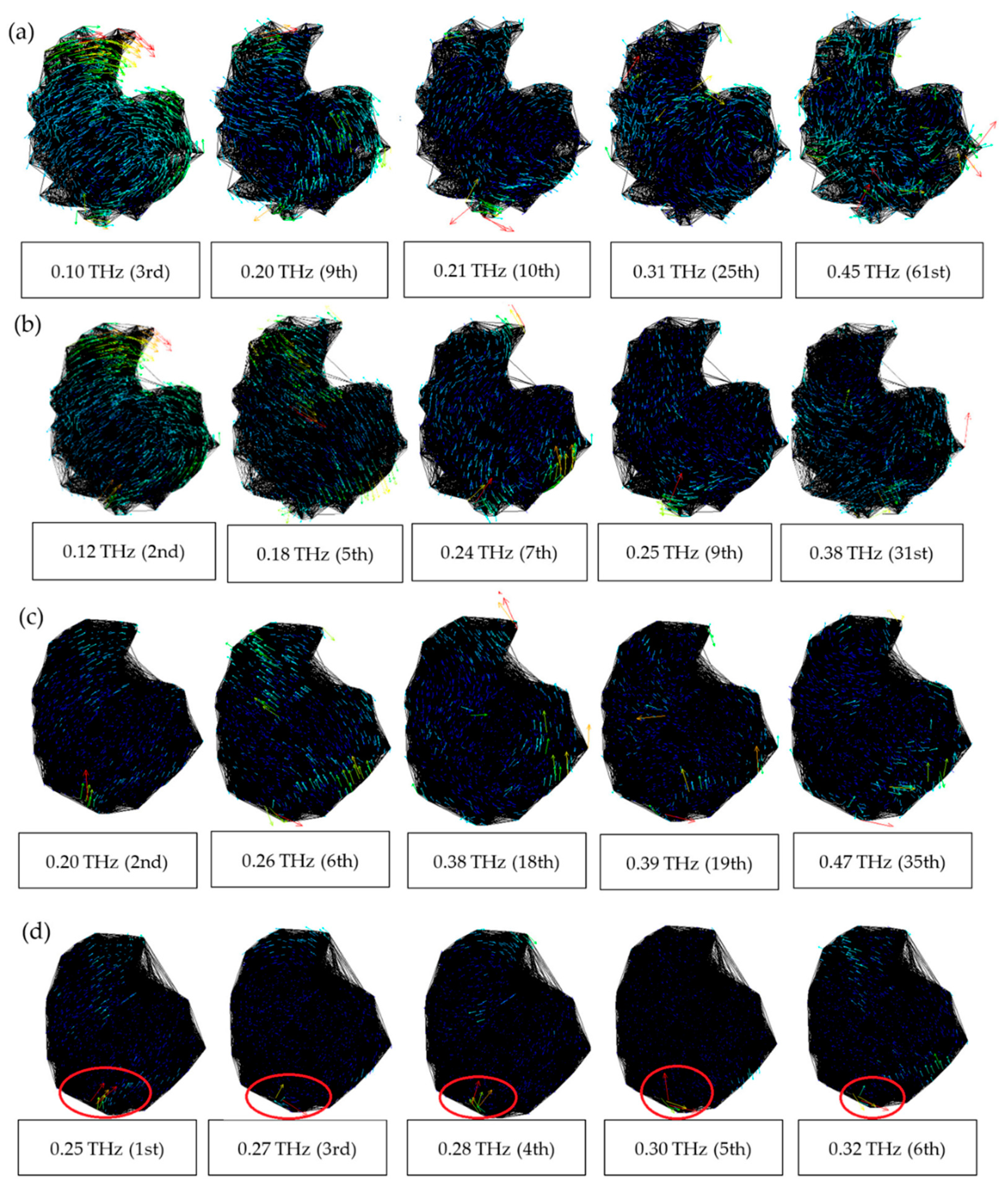
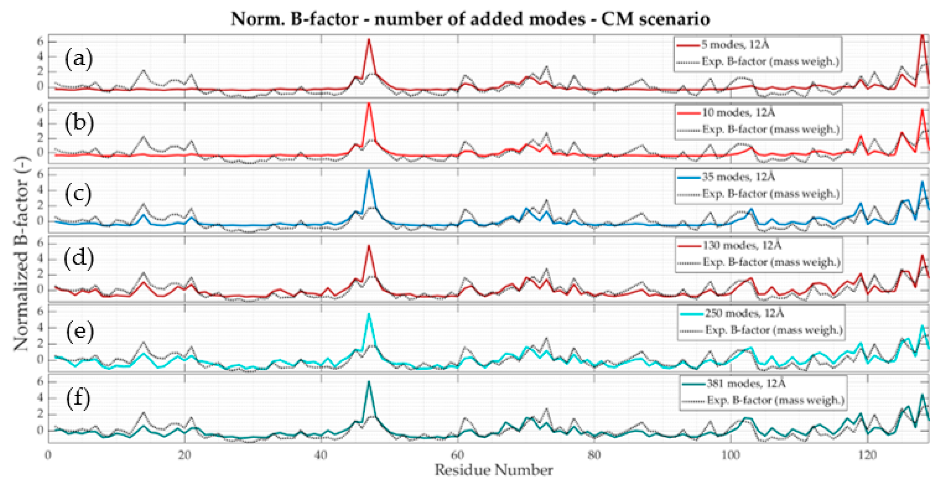
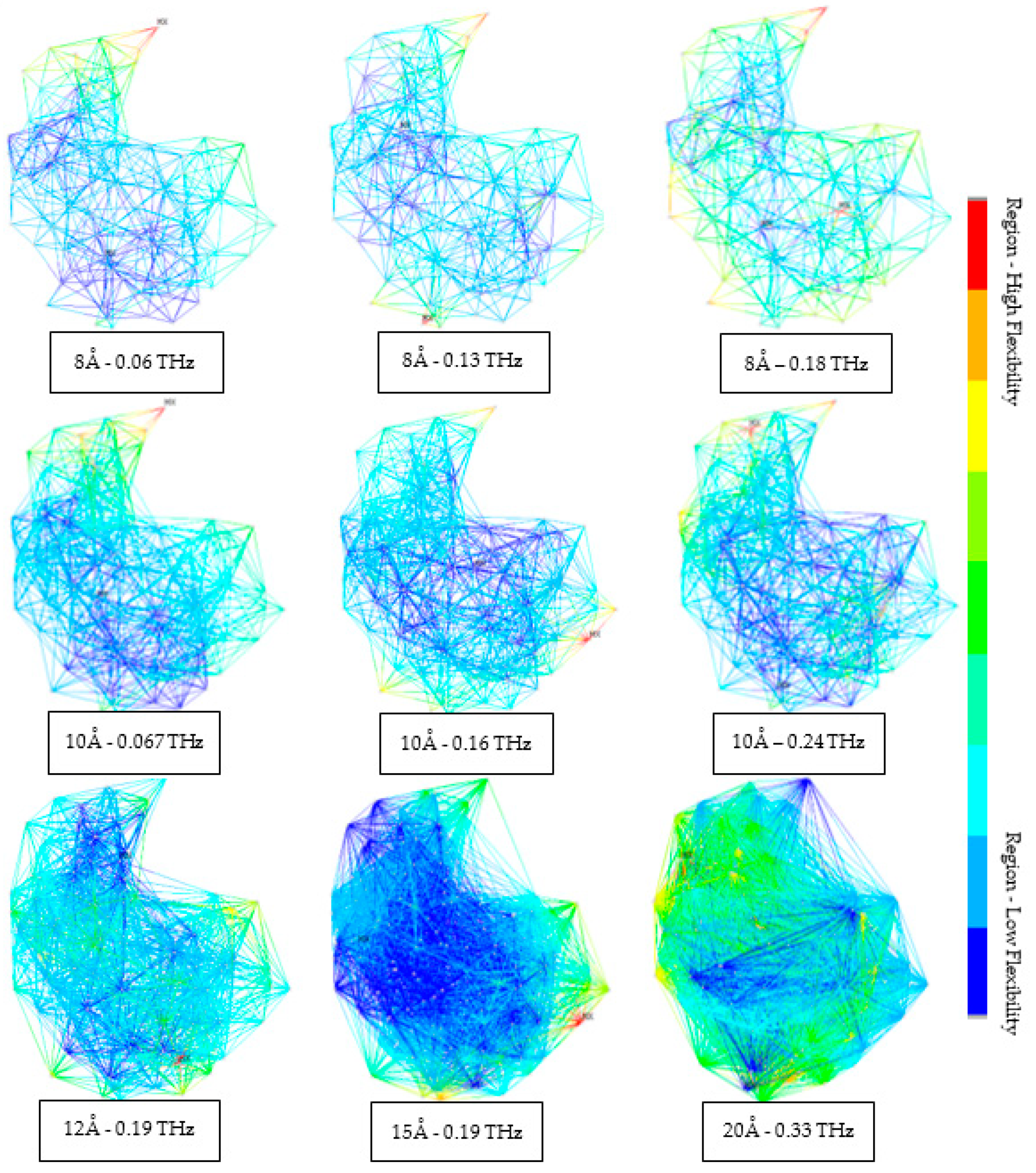
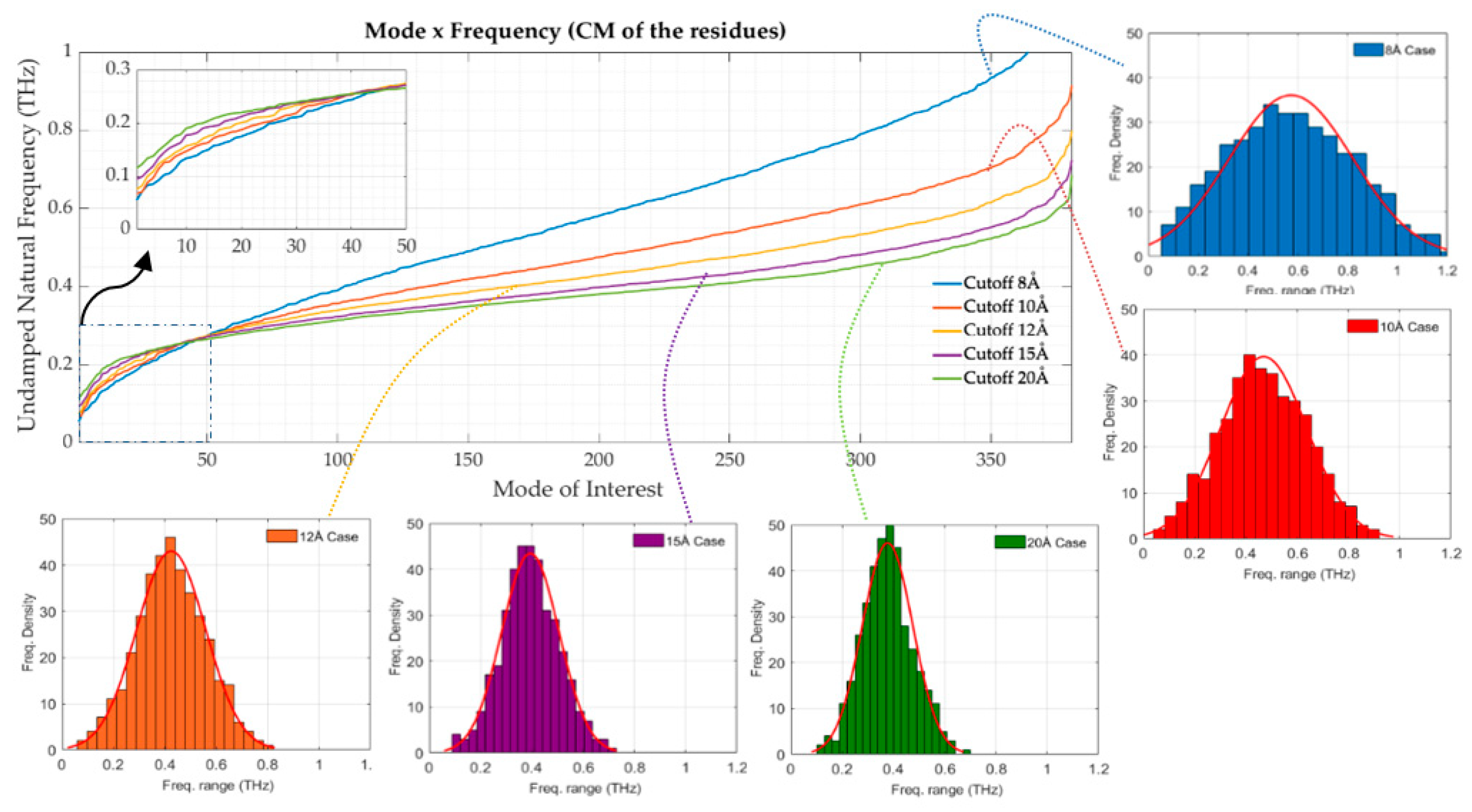
3.2. Coarse-Grained Model

The mass-weighted experimental B-factors in the CM of each residue were used as reference values to compute the axial rigidity EA of the elastic connections generated for the coarse-grained model. Similar to what occurs in the all-atom model, this procedure is performed to establish a comparison between the B-factors’ numerical and experimental values, and the resulting value of EA leads to a not negligible influence on the obtained frequency values.

Table 2. The defined axial rigidity and stiffness for each case. The values were selected to match the average B-factors extracted experimentally.

Cutoff (Å)	Axial Rigidity EA-CM (N)	Nº of Connections	Average Stiffness k (N/m)	Axial Rigidity EA-Cα (N) [15]
8	4.56 × 10−10	627	0.783	8.31 × 10−10
10	1.95 × 10−10	1109	0.283	2.35 × 10−10
12	1.13 × 10−10	1771	0.142	1.24 × 10−10
15	0.69 × 10−10	2938	0.0723	0.71 × 10−10
20	0.45 × 10−10	5043	0.0382	0.45 × 10−10

shows the axial rigidity and average stiffness values for each cutoff value. Again, the mean rigidity is found to decrease as the number of connections increases.

The work of Scaramozzino et al. [15] considers the mass of each residue centered at the C^α location and with a constant value throughout the protein structure. In Table 2, we can see that using the CM, the axial rigidity is lower for smaller cutoffs. This effect results from a reduced standard deviation of the B-factors when using a CM-based description, which in turn allows reducing the individual rigidity values to obtain the same averaged B-factor. As an example, the 8 Å case was found to provide a standard deviation of 28% lower for the B-factor curves using the CM, with respect to the C^α representation. On the other side, for higher cutoffs, e.g., 20 Å, the variation is reduced, leading to almost the same values for both methods. From this observation, it can be concluded that the proposed change has a more significant impact on the rigidity values for the cases with a lower number of connections. The construction of a model based on the CM locations stabilizes the structural state decreasing the oscillations in flexible regions. On the other side, for higher cutoffs, the difference using the CM and the C^α scenarios is lower. In terms of flexibility, the higher number of connections imposes more restrictions on the system, making the actual position of the nodes less critical.

The normalized B-factors are presented in Figure 8a for all cutoffs applying the data provided in Table 2, with respect to the model based on the CM locations. The comparison is also made with the results of Scaramozzino et al. [15], concerning the model based on the C^α sites, as reported in Figure 8b. From these figures, it is possible to observe less variance between the different numerical curves for the CM-based model. An example can be given by observing what happens at node 117. The peak at 8 Å is not seen for the other C^α-based cutoffs when compared to the CM-based models. Therefore, the application of the CM modeling technique appears to smooth the jump between the different horizons and provide more robustness to the model, i.e., less dependence on the specific cutoff value. Furthermore, it seems that the application of the CM-based scheme also allows smoothing the highest peaks that are found in the C^α-based numerical B-factors (see Figure S1 in the Supplementary Material).

The Pearson correlation coefficient between the numerical and experimental B-factors is then used to confirm the previous comments and it also allows us to establish the agreement between the curves quantitatively. In Figure 9a, the correlation coefficient among each numerical solution and with the C^α experimental B-factors are reported. The same output is presented in Figure 9b for the CM-based scenario. From the analysis of the obtained Pearson coefficients, the previous arguments are confirmed. For example, the correlation among the generated numerical models with 20 Å and 8 Å cutoff increases from 0.816 for the C^α-based models to 0.882 for the CM-based ones. The remaining values of the correlation coefficients among the various numerical solutions show similar behavior. Therefore, it follows that using the CM locations as the nodes of the truss-like structure leads to fewer dependencies of the results on the specific cutoff value. Additionally, the difference between experimental and numerical values also has less influence in the CM-based scenario. For example, the coefficient gap between 8 Å and 20 Å is 60% lower for the CM-based approach.

Similar to Figure 4, the effect of the number of modes for evaluating the numerical B-factors has been investigated for the 12 Å case of the coarse-grained model. Figure 10a reports the computed B-factors by adopting only the lowest 5 modes. The following plots, i.e., Figure 10b–f, show the case when 10, 35, 130, 250, and all 381 modes are considered, respectively. Similar to what was found for the all-atom model, the initial low-frequency modes are not sufficient to represent the curve of experimental B-factors alone. However, the convergence towards the final profile obtained with all 381 modes in the coarse-grained representation is faster, and a lower number of modes is needed to reach the final curve. Note that, after adding the first 130 modes, the profile basically does not show any additional significant changes.

Figure 11 displays the collectivity index for the coarse-grained structure for the CM-based scenario. Smaller cutoffs produce index values around 0.9 for a large portion of the frequency spectrum, meaning that highly collective motions can be detected when using the coarse-grained strategy. On the other side, as the cutoff increases, the curves’ overall behavior translates downwards (similarly to what is found in the all-atom models), reducing the collectivity of the motions. The same behavior was found considering the C^α-based configuration (see Figure S2 in the Supplementary Material).

The highest collectivity values are marked with a dashed-red line and the respective mode shapes are represented in Figure 12. The illustrated nine cases indicate the protein regions with high (red) and low (blue) flexibility. Cutoffs of 15 Å and 20 Å have a diffuse distribution of motions without global motions. This is caused because, for higher cutoff values, the protein’s inner regions are highly constrained by many connections, allowing only local movements at the structure’s external parts. On the other side, for the 8 Å case, the complete system has the freedom to vibrate for a wide range of frequencies, demonstrating many cooperative modes.

Finally, Figure 13 shows the frequency spectrum for all modes and selected cutoffs for the CM-based scheme. The histograms for each curve are also added, which indicate a change in shape with the increasing cutoff value. The dispersion decreases while a normal distribution becomes more evident for the cutoffs of 12 Å. Note that adopting the coarse-grained strategy, the Gaussian distribution of the frequency values is more prominent for all selected cutoffs than the previously analyzed distributions for the all-atom model (see Figure 7).

4. Conclusions

The application of a network of links interconnecting nodes that mimic the protein atoms (all-atom model) or residues (coarse-grained model) was studied in this work. The static geometrical description made available in the PDB file for the crystallized hen-egg white lysozyme was used to analyze the dynamic properties of the resulting structure. Each node was interconnected with close neighbors by establishing a sphere of influence, i.e., a cutoff radius that defines the connectivities. The all-atom geometry was composed of 1000 heavy atoms, while the coarse-grained domain comprised the 129 amino acids of the protein. Various conventional dynamic properties were extracted and analyzed with different tools.

Regarding the application of the all-atom model, it was found that the computed B-factors displayed an overall behavior similar to the experimental ones. Some spurious peaks were created, but the protein flexibility was globally well captured with this modeling technique. The effect of the number of eigenvectors considered in the B-factor summation process was also investigated and discussed. It was found that the application of only the initial low-frequency modes is not necessarily sufficient enough to capture all the significant peaks. It was shown that more than half of the 2994 extracted modes should be used to obtain a good approximation with the experimental values when using the all-atom representation.

The collectivity index analysis showed that the modes are relatively localized with the all-atom modeling strategy. Additionally, it was observed that the mode shapes do depend on the selected horizon. However, lower cutoffs presented the classic cleft mode observed in many other studies. From the 15 Å case onwards, this specific modal shape was lost, and collective motions were also reduced. Therefore, it seems that increasing the number of elastic connections creates a locking process that only allows localized movements to occur in single modes.

The range of frequencies from the first mode up to the last one was found to span within one order of magnitude. Moreover, it was observed that all the 2994 natural frequencies were highly packed. The increase of the adopted cutoff value was found to increase the structure’s global stiffness, reducing even further the spanning of the full frequency range. These frequency spectra tended to follow a clear normal distribution for the cases between 12 Å and 15 Å. The literature indicates this behavior due to the similar form and constituents composing globular proteins. However, the reasons for the presence of a normal distribution are still in debate without a clear answer to that. This discussion can be deepened in future studies.

Regarding the application of the coarse-grained model, it was found that the application of the real residue masses to the structure’s nodes, which correspond to the actual masses of each amino acid, did not lead to significant changes in the dynamic output. By comparison with the previous work from Scaramozzino et al. [15], who considered a uniform mass for all the residues, no significant difference was found as far as the mode shapes and B-factors profiles were concerned. This leads to conclude that the structure’s mass is reasonably uniformly distributed within a globular protein; therefore, there is no need to consider the actual mass values when adopting a coarse-grained modeling approach.

The main divergence from the previous work originated when considering a different location for the node representing each amino acid within the structure. The usual strategy for this purpose has relied on the node’s location at the position of the C^α atom [8,9,10,15]. In this work, we considered the case where the representative node is placed at the Center of Mass (CM) of each amino acid. This strategy was found to cause lower local flexibility, leading to lower values of the adopted axial stiffness, especially for the models with smaller cutoff. Consequently, the B-factor profiles were found to be more robust for changes in the cutoff value, which might allow extracting properties that have fewer dependencies on the applied sphere of influence. Other coarse-graining mapping strategies, where the position of the beads depends on the biochemical features of the amino acids, might as well be investigated. However, the overall low-frequency dynamics of the protein is not expected to change drastically, as the three-dimensional shape of the protein structure remains basically the same.

The collectivity index was applied for the coarse-grained model as well, and the analysis showed that more collective, i.e., global motions, can be detected when using a coarse-grained strategy. Nevertheless, specific mode shapes also depend on the selected cutoff value. Finally, the spectral distributions of the natural frequencies were investigated for the adopted cutoff values, and again the characteristic Gaussian behavior was clearly found in the frequency distribution.

It has to be noted that in the present analysis, a single conformation of the lysozyme at the fixed temperature of 293 K (PDB code: 4YM8) was investigated. However, the conformation of the protein can depend on the value of the temperature at which the X-ray experimental takes place, and so do the values of the B-factors [59]. Therefore, the investigation of multiple conformations at different temperatures might reveal slightly different outcomes regarding protein flexibility and the obtained vibrational frequencies, which will be the object of future studies. Nevertheless, the advantage of the presented approach, which is common to all ENMs [7,9,10], is that all crystal structures obtained at different temperatures can be directly taken as the structures corresponding to the energy minimum and undergo the same calculations presented above. The effect of temperature will thus be taken into account: (1) implicitly, by considering a different temperature-dependent crystal structure and (2) explicitly, by calculating the absolute values of the B-factors with the selected value of temperature, as reported in Equation (8).

References

1. Bahar, I.; Jernigan, R.L.; Dill, K.A. Protein Actions: Principles & Modeling; Garland Science: New York, NY, USA, 2017. [Google Scholar]
2. Alberts, B.; Johnson, A.; Lewis, J.; Morgan, D.; Raff, M.; Roberts, K.; Walter, P. Molecular Biology of the Cell, 6th ed.; Garland Science: New York, NY, USA, 2002. [Google Scholar]
3. Anfinsen, C.B. Principles that govern the folding of protein chains. Science 1973, 181, 223–230. [Google Scholar] [CrossRef] [PubMed] [Green Version]
4. Bahar, I.; Rader, A.J. Coarse-grained normal mode analysis in structural biology. Curr. Opin. Struct. Biol. 2005, 15, 586–592. [Google Scholar] [CrossRef] [PubMed] [Green Version]
5. Liwo, A. Computational Methods to Study the Structure and Dynamics of Biomolecules and Biomolecular Processes; Springer: Berlin/Heidelberg, Germany, 2014; ISBN 978-3-642-28553-0. [Google Scholar]
6. Levitt, M.; Sander, C.; Stern, P.S. Protein normal-mode dynamics: Trypsin inhibitor, crambin, ribonuclease and lysozyme. J. Mol. Biol. 1985, 181, 423–447. [Google Scholar] [CrossRef]
7. Tirion, M.M. Large amplitude elastic motions in proteins from a single-parameter, atomic analysis. Phys. Rev. Lett. 1996, 77, 1905–1908. [Google Scholar] [CrossRef] [PubMed]
8. Haliloglu, T.; Bahar, I.; Erman, B. Gaussian dynamics of folded proteins. Phys. Rev. Lett. 1997, 79, 3090. [Google Scholar] [CrossRef]
9. Bahar, I.; Atilgan, A.R.; Erman, B. Direct evaluation of thermal fluctuations in proteins using a single-parameter harmonic potential. Fold. Des. 1997, 2, 173–181. [Google Scholar] [CrossRef] [Green Version]
10. Atilgan, A.R.; Durell, S.R.; Jernigan, R.L.; Demirel, M.C.; Keskin, O.; Bahar, I. Anisotropy of fluctuation dynamics of proteins with an elastic network model. Biophys. J. 2001, 80, 505–515. [Google Scholar]
11. Tama, F.; Gadea, F.X.; Marques, O.; Sanejouand, Y.H. Building-block approach for determining low-frequency normal modes of macromolecules. Proteins Struct. Funct. Genet. 2000, 41, 1–7. [Google Scholar] [CrossRef] [Green Version]
12. Yang, L.; Song, G.; Jernigan, R.L. Protein elastic network models and the ranges of cooperativity. Proc. Natl. Acad. Sci. USA 2009, 106, 12347–12352. [Google Scholar] [CrossRef] [Green Version]
13. Eyal, E.; Yang, L.W.; Bahar, I. Anisotropic network model: Systematic evaluation and a new web interface. Bioinformatics 2006, 22, 2619–2627. [Google Scholar] [CrossRef]
14. Hoffmann, A.; Grudinin, S. NOLB: Nonlinear Rigid Block Normal-Mode Analysis Method. J. Chem. Theory Comput. 2017, 13, 2123–2134. [Google Scholar] [CrossRef] [PubMed]
15. Scaramozzino, D.; Lacidogna, G.; Piana, G.; Carpinteri, A. A finite-element-based coarse-grained model for global protein vibration. Meccanica 2019, 54, 1927–1940. [Google Scholar] [CrossRef]
16. Song, G.; Jernigan, R.L. An enhanced elastic network model to represent the motions of domain-swapped proteins. Proteins Struct. Funct. Genet. 2006, 63, 197–209. [Google Scholar] [CrossRef] [PubMed]
17. Na, H.; Jernigan, R.L.; Song, G. Bridging between NMA and Elastic Network Models: Preserving All-Atom Accuracy in Coarse-Grained Models. PLoS Comput. Biol. 2015, 11, e1004542. [Google Scholar] [CrossRef] [PubMed]
18. Tama, F.; Sanejouand, Y.H. Conformational change of proteins arising from normal mode calculations. Protein Eng. 2001, 14, 1–6. [Google Scholar] [CrossRef] [PubMed]
19. Yang, L.; Song, G.; Jernigan, R.L. How well can we understand large-scale protein motions using normal modes of elastic network models? Biophys. J. 2007, 93, 920–929. [Google Scholar] [CrossRef] [PubMed] [Green Version]
20. Zimmermann, M.T.; Kloczkowski, A.; Jernigan, R.L. MAVENs: Motion analysis and visualization of elastic networks and structural ensembles. BMC Bioinform. 2011, 12, 1–7. [Google Scholar] [CrossRef] [Green Version]
21. Atilgan, C.; Atilgan, A.R. Perturbation-response scanning reveals ligand entry-exit mechanisms of ferric binding protein. PLoS Comput. Biol. 2009, 5, e1000544. [Google Scholar] [CrossRef] [Green Version]
22. Atilgan, C.; Gerek, Z.N.; Ozkan, S.B.; Atilgan, A.R. Manipulation of conformational change in proteins by single-residue perturbations. Biophys. J. 2010, 99, 933–943. [Google Scholar] [CrossRef] [Green Version]
23. Liu, J.; Sankar, K.; Wang, Y.; Jia, K.; Jernigan, R.L. Directional Force Originating from ATP Hydrolysis Drives the GroEL Conformational Change. Biophys. J. 2017, 112, 1561–1570. [Google Scholar] [CrossRef] [Green Version]
24. Scaramozzino, D.; Khade, P.M.; Jernigan, R.L.; Lacidogna, G.; Carpinteri, A. Structural Compliance: A New Metric for Protein Flexibility. Proteins Struct. Funct. Bioinform. 2020, 88, 1482–1492. [Google Scholar]
25. Kurkcuoglu, O.; Jernigan, R.L.; Doruker, P. Collective dynamics of large proteins from mixed coarse-grained elastic network model. QSAR Comb. Sci. 2005, 24, 443–448. [Google Scholar] [CrossRef]
26. Mishra, S.K.; Jernigan, R.L. Protein dynamic communities from elastic network models align closely to the communities defined by molecular dynamics. PLoS ONE 2018, 13, e0199225. [Google Scholar] [CrossRef] [PubMed]
27. Yang, L.; Song, G.; Carriquiry, A.; Jernigan, R.L. Close Correspondence between the Essential Protein Motions from Principal Component Analysis of Multiple HIV-1 Protease Structures and Elastic Network Modes. Structure 2008, 16, 321–330. [Google Scholar] [CrossRef] [PubMed] [Green Version]
28. Sankar, K.; Mishra, S.K.; Jernigan, R.L. Comparisons of Protein Dynamics from Experimental Structure Ensembles, Molecular Dynamics Ensembles, and Coarse-Grained Elastic Network Models. J. Phys. Chem. B 2018, 122, 5409–5417. [Google Scholar] [CrossRef] [PubMed] [Green Version]
29. Acbas, G.; Niessen, K.A.; Snell, E.H.; Markelz, A.G. Optical measurements of long-range protein vibrations. Nat. Commun. 2014, 5, 1–7. [Google Scholar]
30. Niessen, K.A.; Xu, M.; Paciaroni, A.; Orecchini, A.; Snell, E.H.; Markelz, A.G. Moving in the Right Direction: Protein Vibrational Steering Function. Biophys. J. 2017, 112, 933–942. [Google Scholar] [CrossRef] [Green Version]
31. Whitmire, S.E.; Wolpert, D.; Markelz, A.G.; Hillebrecht, J.R.; Galan, J.; Birge, R.R. Protein flexibility and conformational state: A comparison of collective vibrational modes of wild-type and D96N bacteriorhodopsin. Biophys. J. 2003, 85, 1269–1277. [Google Scholar] [CrossRef] [Green Version]
32. Carpinteri, A.; Lacidogna, G.; Piana, G.; Bassani, A. Terahertz mechanical vibrations in lysozyme: Raman spectroscopy vs. modal analysis. J. Mol. Struct. 2017, 1139, 222–230. [Google Scholar] [CrossRef]
33. Lacidogna, G.; Piana, G.; Bassani, A.; Carpinteri, A. Raman spectroscopy of Na/K-ATPase with special focus on low-frequency vibrations. Vib. Spectrosc. 2017, 92, 298–301. [Google Scholar]
34. Carpinteri, A.; Piana, G.; Bassani, A.; Lacidogna, G. Terahertz vibration modes in Na/K-ATPase. J. Biomol. Struct. Dyn. 2019, 37, 256–264. [Google Scholar] [PubMed]
35. Turton, D.A.; Senn, H.M.; Harwood, T.; Lapthorn, A.J.; Ellis, E.M.; Wynne, K. Terahertz underdamped vibrational motion governs protein-ligand binding in solution. Nat. Commun. 2014, 5, 2–7. [Google Scholar] [CrossRef] [PubMed] [Green Version]
36. Berman, H.M.; Westbrook, J.; Feng, Z.; Gilliland, G.; Bhat, T.N.; Weissig, H.; Shindyalov, I.N. The Protein Data Bank. Nucleic Acids Res. 2000, 28, 235–242. [Google Scholar] [CrossRef] [PubMed] [Green Version]
37. Brown, K.G.; Erfurth, S.C.; Small, E.W.; Peticolas, W.L. Conformationally dependent low-frequency motions of proteins by laser Raman spectroscopy. Proc. Natl. Acad. Sci. USA 1972, 69, 1467–1469. [Google Scholar] [CrossRef] [Green Version]
38. Painter, P.C.; Mosher, L.; Rhoads, C. Low-frequency modes in the raman spectra of proteins. Biopolymers 1982, 21, 1469–1472. [Google Scholar]
39. Genzel, L.; Keilmann, F.; Martin, T.P.; Wintreling, G.; Yacoby, Y.; Fröhlich, H.; Makinen, M.W. Low-frequency Raman spectra of lysozyme. Biopolymers 1976, 15, 219–225. [Google Scholar] [CrossRef]
40. Rygula, A.; Majzner, K.; Marzec, K.M.; Kaczor, A.; Pilarczyk, M.; Baranska, M. Raman spectroscopy of proteins: A review. J. Raman Spectrosc. 2013, 44, 1061–1076. [Google Scholar]
41. Thomas, G.J. Raman spectroscopy of protein and nucleic acid assemblies. Annu. Rev. Biophys. Biomol. Struct. 1999, 28, 1–27. [Google Scholar]
42. Bunaciu, A.A.; Aboul-Enein, H.Y.; Hoang, V.D. Raman spectroscopy for protein analysis. Appl. Spectrosc. Rev. 2015, 50, 377–386. [Google Scholar] [CrossRef]
43. Bertoldo Menezes, D.; Reyer, A.; Yüksel, A.; Bertoldo Oliveira, B.; Musso, M. Introduction to Terahertz Raman spectroscopy. Spectrosc. Lett. 2018, 51, 438–445. [Google Scholar]
44. Ferreira, A.J.M. Matlab Codes for Finite Element Analysis, Solid and Structures; Springer: Berlin/Heidelberg, Germany, 2009. [Google Scholar]
45. Montáns, F.J.; Muñoz, I. Dynamic Analysis of Structures for the Finite Element Method. 2013. [Google Scholar]
46. Creighton, T.E. Proteins: Structures and Molecular Properties, 2nd ed.; Freeman, W.H., Ed.; Macmillan: New York, NY, USA, 1993. [Google Scholar]
47. Sun, Z.; Liu, Q.; Qu, G.; Feng, Y.; Reetz, M.T. Utility of B-Factors in Protein Science: Interpreting Rigidity, Flexibility, and Internal Motion and Engineering Thermostability. Chem. Rev. 2019, 119, 1626–1665. [Google Scholar] [CrossRef]
48. Karplus, P.A.; Schulz, G.E. Prediction of chain flexibility in proteins—A tool for the selection of peptide antigens. Naturwissenschaften 1985, 72, 212–213. [Google Scholar] [CrossRef]
49. Schlessinger, A.; Rost, B. Protein flexibility and rigidity predicted from sequence. Proteins Struct. Funct. Bioinform. 2005, 61, 115–126. [Google Scholar] [CrossRef] [PubMed] [Green Version]
50. Vihinen, M.; Torkkila, E.; Riikonen, P. Accuracy of protein flexibility predictions. Proteins Struct. Funct. Bioinform. 1994, 19, 141–149. [Google Scholar] [CrossRef] [PubMed]
51. Kuczera, K.; Kuriyan, J.; Karplus, M. Temperature dependence of the structure and dynamics of myoglobin. A simulation approach. J. Mol. Biol. 1990, 213, 351–373. [Google Scholar] [CrossRef]
52. Feyfant, E.; Sali, A.; Fiser, A. Modeling mutations in protein structures. Protein Sci. 2007, 16, 2030–2041. [Google Scholar] [CrossRef] [Green Version]
53. Carugo, O. Maximal B-factors in protein crystal structures. BMC Bioinform. 2018, 19, 61. [Google Scholar] [CrossRef]
54. Khade, P.; Kumar, A.; Jernigan, R.L. Characterizing and predicting protein hinges for mechanistic insight. J. Mol. Biol. 2020, 432, 508–522. [Google Scholar]
55. Dykeman, E.C.; Sankey, O.F. Normal mode analysis and applications in biological physics. J. Phys. Condens. Matter 2010, 22, 423202. [Google Scholar]
56. Prompers, J.J.; Lienin, S.F.; Brüschweiler, R. Collective reorientational motion and nuclear spin relaxation in proteins. Pacific Symp. Biocomput. 2001, 88, 79–88. [Google Scholar]
57. Brooks, B.; Karplus, M. Harmonic dynamics of proteins: Normal modes and fluctuations in bovine pancreatic trypsin inhibitor. Proc. Natl. Acad. Sci. USA 1983, 80, 6571–6575. [Google Scholar] [CrossRef] [PubMed] [Green Version]
58. Ben-Avraham, D. Vibrational normal-mode spectrum of globular proteins. Phys. Rev. B 1993, 47, 14559–14560. [Google Scholar] [CrossRef] [PubMed]
59. Russi, S.; Gonzalez, A.; Kenner, L.R.; Keedy, D.A.; Fraser, J.S.; van den Bedem, H. Conformational variation of protein at room is not dominated by radiation damage. J. Syncrothron Radiat. 2017, 24, 73–82. [Google Scholar] [CrossRef] [PubMed]
Figure 1. (a) The ribbon structure of the hen-egg white lysozyme (PBD code: 4YM8); (b) all carbon, nitrogen, oxygen, and sulfur atoms and their covalent bonds; (c) the 129 nodes and the indication of the cutoff (sphere of influence) which is used to generate the elastic connections in the coarse-grained model.
Applsci 11 00547 g001
Figure 2. The numerical and experimental B-factor for all cases under analysis. The vertical lines indicate the Cα nodes. The experimental B-factors are shown with dotted-black lines. Three plots are displayed to avoid overlapping and facilitate visualization: (a) 4, 6, 8; (b) 10, 12, 15; (c) 20, 25, and 30 Å. Additionally, three sections are amplified for a better view of specific regions of the protein.
Applsci 11 00547 g002
Figure 3. The Pearson correlation coefficient between the different numerical B-factors and with the experimental ones for the all-atom scheme.
Applsci 11 00547 g003
Figure 4. The numerical and experimental B-factor for the 12 Å case. The plots vary the number of modes added for the B-factor calculation. At (a) 10 modes, (b) 50 modes, (c) 300 modes, (d) 1000 modes, (e) 2000 modes, and (f) 2994 modes.
Applsci 11 00547 g004
Figure 5. The mode collectivity index κ for all cutoff values according to the respective natural frequency range. The red dashed lines indicate the modes represented in Figure 6 for 6, 8, 12, and 15 Å cases related to the most significant collective motions.
Applsci 11 00547 g005
Figure 6. Representation of the modes with the highest collectivity index displayed in Figure 5. Cases represented are for: (a) 6 Å, (b) 8 Å, (c) 12 Å and (d) 15 Å.
Applsci 11 00547 g006
Figure 7. The frequency density distribution for the all-atom scheme and the corresponding modes for the whole spectrum of 2994 frequencies. A closer view of the initial 250 modes is also presented at the top-left.
Applsci 11 00547 g007
Figure 8. (a) The center of mass (CM) of each amino acid is taken to calculate the numerical B-factors. The experimental value is also weighted according to the mass of each atom composing the residue. (b) The results from Scaramozzino et al. [15] considering the Cα location.
Applsci 11 00547 g008
Figure 9. The Pearson coefficient comparing different numerical solutions and with the experimental B-factors. (a) Adopting the Cα scheme. (b) Adopting the CM-based strategy.
Applsci 11 00547 g009
Figure 10. The numerical and experimental B-factor for the 12 Å case. The plots vary the number of modes added for the B-factor calculation. At (a) 5 modes, (b) 10 modes, (c) 35 modes, (d) 130 modes, (e) 250 modes and (f) 381 modes.
Applsci 11 00547 g010
Figure 11. The mode collectivity index κ for the coarse-grained model with the CM-based configuration. The x-axis represents the frequency spectrum for each cutoff. The red dashed lines indicate the most collective modes described in Figure 12 for 8, 10, 12, and 15 Å cases.
Applsci 11 00547 g011
Figure 12. Examples of mode shapes with high global motions according to the collectivity index presented in Figure 11 (red dashed lines). The CM-based scenario is addressed.
Applsci 11 00547 g012
Figure 13. The modes and the natural frequencies for the whole spectrum of 381 modes. All cases based on the different cutoffs are displayed. A closer view of the first 50 modes is also presented at the top-left of the main plot. The six histograms show the frequency distribution for each cutoff.
Applsci 11 00547 g013