
Forecasting Taxi Demands Using Generative Adversarial Networks with Multi-Source Data


School of Digital Media, Nanyang Institute of Technology, Chang Jiang Road No. 80, Nanyang 473004, China
*
Author to whom correspondence should be addressed.
Appl. Sci. 2021, 11(20), 9675; https://0-doi-org.brum.beds.ac.uk/10.3390/app11209675
Submission received: 23 August 2021
/
Revised: 27 September 2021
/
Accepted: 6 October 2021
/
Published: 17 October 2021
(This article belongs to the Special Issue Future Transportation)
Abstract
:As a popular transportation mode in urban regions, taxis play an essential role in providing comfortable and convenient services for travelers. For the sake of tackling the imbalance between supply and demand, taxi demand forecasting can help drivers plan their routes and reduce waiting time and oil pollution. This paper proposes a deep learning-based model for taxi demand forecasting with multi-source data using Generative Adversarial Networks. Firstly, main features were extracted from multi-source data, including GPS taxi data, road network data, weather data, and points of interest. Secondly, Generative Adversarial Network, comprised of the recurrent network model and the conventional network model, is adopted for fine-grained taxi demand forecasting. A comprehensive experiment is conducted based on a real-world dataset of the city of Wuhan, China. The experimental results showed that our model outperforms state-of-the-art prediction methods and validates the usefulness of our model. This paper provides insights into the temporal, spatial, and external factors in taxi demand-supply equilibrium based on the results. The findings can help policymakers alter the taxi supply and the taxi lease rents for periods and increase taxi profit.
1. Introduction
Taxis play a vital role in the modern urban transportation system as they comfortably and conveniently serve many urban passengers. According to the annual report of urban passenger transport operation [1], more than 216 million passengers used a taxi service in 2020 in Wuhan city. However, a critical challenge emerged that there is a significant mismatch between the supply of taxis and passengers’ demands. For instance, passengers may not find taxis for an extended period in an area at a specific time. In contrast, taxi drivers may cruise roads without getting passengers in another area at the same time. Therefore, this may lead to several problems, such as increasing passengers’ wait time and oil consumption and decreasing taxi incomes. To this end, it becomes significant to accurately predict fine-grained taxi demands in advance to guide taxi drivers to areas with high demands [2].
There is a need for a deep understanding of the temporally varying taxi-passenger demand over various spatial areas that can guide and motivate drivers to be in the areas with a high potential of passenger demands and thus enhance the taxis’ utilization rate [3].
Recently, there has been much research investigating the correlation between taxi demands and related dependencies. However, taxi demand forecasting is still an open problem, which is mainly affected by several kinds of factors [4,5,6]:
- (1)
- Temporal factors include weekdays, weekends, rush hours, holidays.
- (2)
- Spatial factors such as neighboring areas.
- (3)
- External factors including POI data, weather, traffic condition, etc.
In this study, we try to study taxi demands and related factors extracted from multi-source data. The taxi demands, represented by taxi pick-up events, were analyzed using a generative adversarial networks (GAN) to forecast taxi-passenger demand by considering significant factors, including temporal, spatial, and external factors. A novel deep learning-based approach is proposed for feature extraction and fine-grained taxi demands forecasting in urban areas.
The main contributions of this article include the following:
- (1)
- To provide a method for extracting features related to taxi demands from multi-source data following a detailed analytic for the relationship between taxi demands and significant factors.
- (2)
- The generative adversarial networks (GAN) model is adopted to perform taxi demand forecasting. In the GAN, the long short-term memory (LSTM) structure is selected in the generative network, whereas the Conventional network is used in the discriminator network to enable the GAN model to deal with fundamental factors and related patterns naturally.
- (3)
- The proposed forecasting model was evaluated using a real multi-source data set collected of Wuhan city, China. The experiments proved that the proposed model showed better results and outperformed other state-of-the-art methods.
The rest of the paper is structured as follows: Section 2 presents a related review of the recent taxi demand prediction methods. Section 3 introduced the mathematical definition of taxi demand forecasting. Section 4 introduces the proposed methodology, followed by explaining the conducted experiment in detail in Section 5. The experimental results are discussed in Section 6. Section 7 concludes the implications and value of taxi demand forecasting findings and introduces the future work.
2. Related Work
Taxi demand forecasting has attracted researchers’ and taxi service companies’ attention due to the massive number of GPS trajectories and the huge spatio-temporal information produced every day by GPS sensors. In general, taxi demands forecasting methods can be categorized into three main classes: traditional methods, machine, and deep learning-based methods.
2.1. Traditional Methods
Traditional methods include statistical and time-series analysis-based methods. Statistical models have been used to study the predicting taxi demands. For instance, Tang et al. [7] developed a probabilistic-based model to predict vehicle trip routes using Hidden Markov Model (HMM). Moreira et al. proposed a data-driven method to predict passengers’ spatial distribution in short-term periods [8]. Liu et al. developed three predictive methods for detecting high hotspots and predicting taxi demands [9]. Chang et al. [10] investigated historical trajectory data to forecast the spatio-temporal patterns of taxi demands.
Time-series analysis-based methods are also considered in traffic data prediction. For example, in [11], the Automatic ARIMA Model is adopted for forecasting the passenger’s hotspot regions using spatio-temporal data. In [12], the authors modeled taxi demand prediction as a time series issue, and an improved ARIMA method is proposed to predict taxi demands by using temporal dependencies. Tong et al. [13] introduced a linear regression-based model along with high-dimensional features to forecasting taxi demands in urban regions.
2.2. Machine and Deep Learning-Based Methods
Markou et al. [14] utilized the information extracted by unstructured data in taxi GPS data and adopted machine learning techniques to forecast taxi demands. In [15], a backpropagation neural network (BPNN) with an extreme gradient boosting (XGB) based method is proposed to predict taxi-hailing demand. In [16], the authors introduced a machine learning-based approach for identifying and predicting the short-term demand for on-demand ride-hailing services. The predicting methodology studied factors related to traffic, trip fare, and weather conditions.
Recently, deep learning-based methods have been popularly adopted in forecasting traffic flow problems. Multi-layer perceptron (MLP), Convolution Neural Network (CNN), Recurrent Neural Network (RNN), and their variation networks have achieved superior achievements in taxi demand prediction.
CNN has been used to forecast traffic flow. For example, Ma et al. [17] split a city into several small grids, transformed city traffic speed into images, and adopted CNN for forecasting traffic speed. Zhang et al. [18] applied CNN by modeling temporal and spatial factors for predicting the traffic flow of bikes in the short-future periods.
The success of RNNs and their enhanced models, such as long short-term memory (LSTM), and gated recurrent units (GRU), led researchers to adopt these methods for predicting traffic flow [5,19,20]. Xu et al. utilized a sequence learning method for predicting future taxi demands in city regions, considering current taxi requests and relevant factors. Mixture density-based recurrent neural networks are developed to investigate historical taxi demand distribution and taxi demand predictions. Rossi in [19] obtained the sequences of historical pick-up and drop-offs and then employed the LSTM network to extract the sequential features for taxi request forecasting. Zhao et al. [20] used a cascaded-based LSTM combined with an origin–destination correlation matrix to capture spatial-temporal patterns. In [10], an LSTM neural network-based method is adopted for forecasting a future pick-demand of a given taxi stand by analyzing the spatial demand of a particular taxi stand and neighboring stands.
To make full use of the spatio-temporal correlation with taxi demands, many researchers combined both CNN and RNN for forecasting traffic flow.
A convolutional-recurrent network-based model is developed for forecasting fine-grained taxi requests [21]. The authors considered various factors related to taxi demands, including the spatial correlations between neighboring areas and function-similar areas, long and short-term periods, and external factors. A context-based attention method combines regions’ predictions to improve the prediction results [22]. Niu et al. [6] used LSTM with CNN in a real-time prediction system by streaming taxi-passenger data. The CNN network is adopted to extract spatial features, whereas LSTM obtained temporal dimensions. Zhang et al. [23] proposed a deep-learning-based model to predict the in-flow and the out-flow of crowds in a city.
Previous works on taxi demand prediction led us to consider historical trip information to forecast future taxi requests. One of the differences between our work and the preceding works is that our model can fill this gap by integrating taxi GPS data with other related historical data sources, including weather conditions, temporal data, POI data, to fully understand taxi supply patterns and consider the significant factors affecting external dependencies of taxi demand simultaneously.
In this research, we employed the generative adversarial networks (GAN) model to forecast taxi demands. In the generative network part, the long short-term memory (LSTM) structure is selected, whereas the Conventional network is used in the discriminator network. Thus, the GAN model (GAN_LSTM_CNN) can deal with the factors included in the Taxi dataset and related patterns perfectly. In addition, and by considering successive iteration and adversarial learning of the discriminator and the generator, we can obtain better prediction results.
3. Problem Definition
In this section, firstly we define several key concepts, and then formally formulate the taxi demand forecasting problem.
- Definition 1 (taxi trip). A taxi trip is defined as a tuple (ID, pickuptime, picklocation,droptime, droplocation, duration, distance, fare), where ID represents the trip identification, pickuptime is the pick-up time (in hours and minutes), picklocation is the pick-up location (longitude and latitude), droptime is the drop-off time, droplocation represents the drop-off location, duration, distance, and fare are the calculated duration, distance and, fare of a trip.
- Definition 2 (Road Network). A road network of a city is composed of a set of road segments. Each road segment is associated with two terminal points (i.e., intersections of crossroads), and connects with other road segments by sharing the same terminals. All road segments compose the road network in the format of a graph.
- Definition 3 (Temporal Data). For the sake of a detailed description of the spatial and temporal dimensions of fine-grained taxi demands, the time is discretized into time slots t (date, hour, and minutes).
- Definition 4 (Point of Interest POI). POI represented a place (like a restaurant) in an urban area r. Each POI pi associated with a location pi.l and a POI category pi.c ∈ C, where C is a set of categories.
- Definition 5 (Weather). Weather presents several parameters related to weather status in a determined time slot (date, hour, and minutes) of an urban area r. Each weather may consider several associated parameters including temperature, humidity, weather status (rain, sunny), wind, etc.
Here, we can provide a formal definition of fine-grained taxi demands as follows.
- Definition 6 (Taxi Demands). We use Yi to represent the amount of taxi pick-ups (demand of taxis) in an area r ∈ R at a time slot t ∈ T. Hence, taxi demands in a time slot t are defined as Yr,t = [Y0,t, Y1,t, …, Yn,t].
To forecast taxi demands in future, we first dig fine-grained taxi demands in past time slots from historical taxi trips data defined as in Definition 1 As Taxi Demands have a strong correlation with other temporal, spatial and external factors, we collect significant factors related to taxi demands (as in Definitions 2,3,4 and 5) in the determined area r, at time slot t.
Now, we can define the problem of forecasting the fine-grained taxi demands in a determined time slot t as follows.
- Definition 7 (Taxi Demand Forecasting Problem). Consider an urban area is divided into disjoint regions R by the road network.
Given fine-grained taxi demands in the past time slots {Yt|t = 0, 1,…,t} extracted from historical taxi trips data (pick-ups), we try to predict fine-grained taxi demands at a determined time slot. The taxi demand forecasting is denoted as t+1 = [1,t+1, …, n,t+1].
4. Methodology
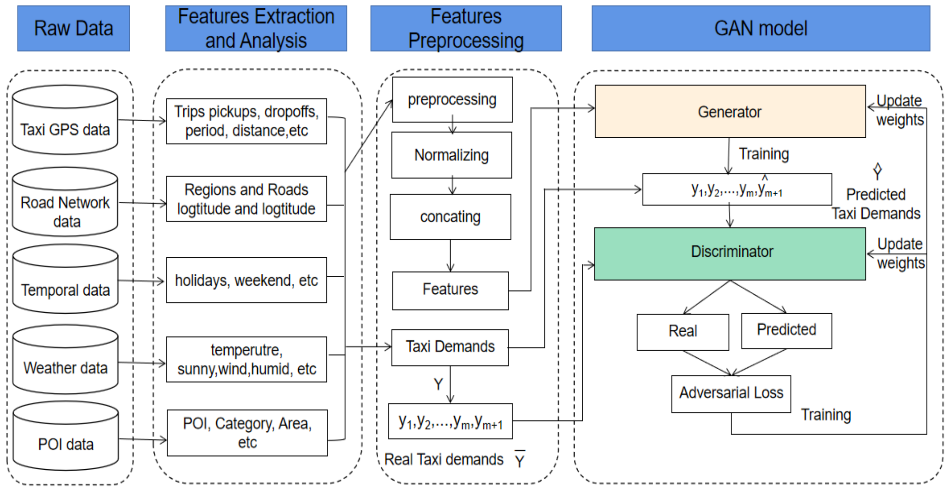
This section introduces the proposed taxi demand forecasting model in detail, including raw data, features extraction and analysis, features pre-processing, and the GAN model. Figure 1 depicts the framework of the proposed model.
4.1. Raw Data
4.1.1. Taxi GPS Data
The dataset used in this paper contains temporally ordered location records collected from 9124 GPS-enabled taxis during 91 days (historical GPS dataset of September, October, and November in 2013) of the city of Wuhan, China.
The temporal resolution of the dataset is 25 s; therefore, approximately 3500 GPS records for a taxi per a day (24 h) would be collected, and the total volume of the dataset approached 320 million records. The GPS meter triggered information to the taxi data center and contains seven taxi attributes, i.e., taxi (driver) ID, timestamp, longitude, latitude, speed, direction, and taxi status. The detailed description of the taxi attributes is shown in Table 1.
4.1.2. Road Network Data
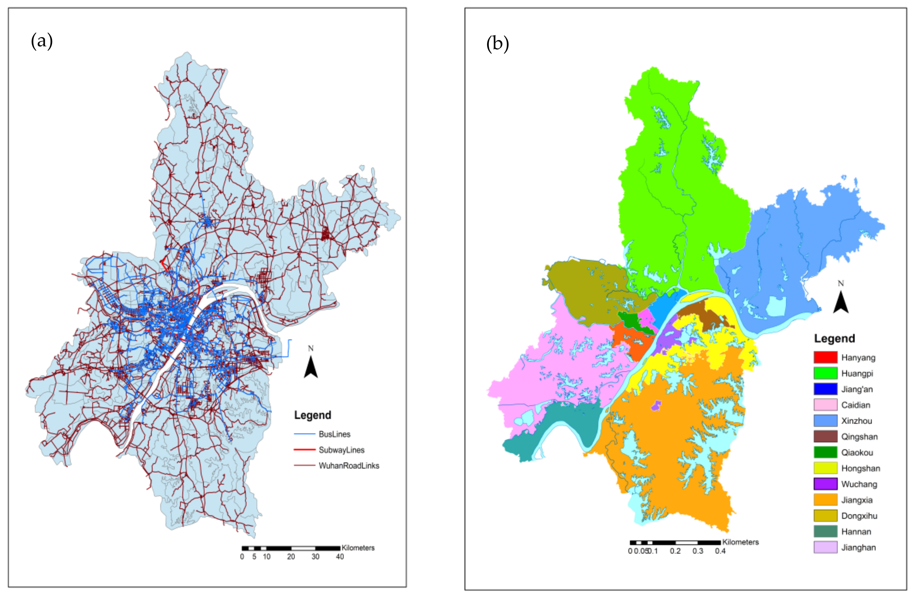
A dataset of the city of Wuhan’s road network obtained from the OpenStreetMap website [24] is used in this research, containing 94,214 intersections and 95,781 road segments. Each road intersection is vectorial, located by related latitude and longitude. The whole area of the city is divided into eight significant regions and 623 disjoint small regions. Figure 2 shows the road network and the central areas in the city of Wuhan, China.
4.1.3. Temporal Data
Besides the taxi GPS data, our study considered temporal data and related factors, including weekday, weekend, holiday, etc., significantly influencing traffic flow and taxi demand distribution.
4.1.4. POI Data
The information of points of interests (POI) may provide useful details about the functions of urban regions relevant to taxi demands. We obtained POI dataset of the city of Wuhan by web data crawler tool (using selenium and PhantomJS in python) from guihuayun website [25] which resulted in collecting approximately 425476 POIs of Wuhan city, grouped into 16 different categories as shown in Table 2.
4.1.5. Weather Data
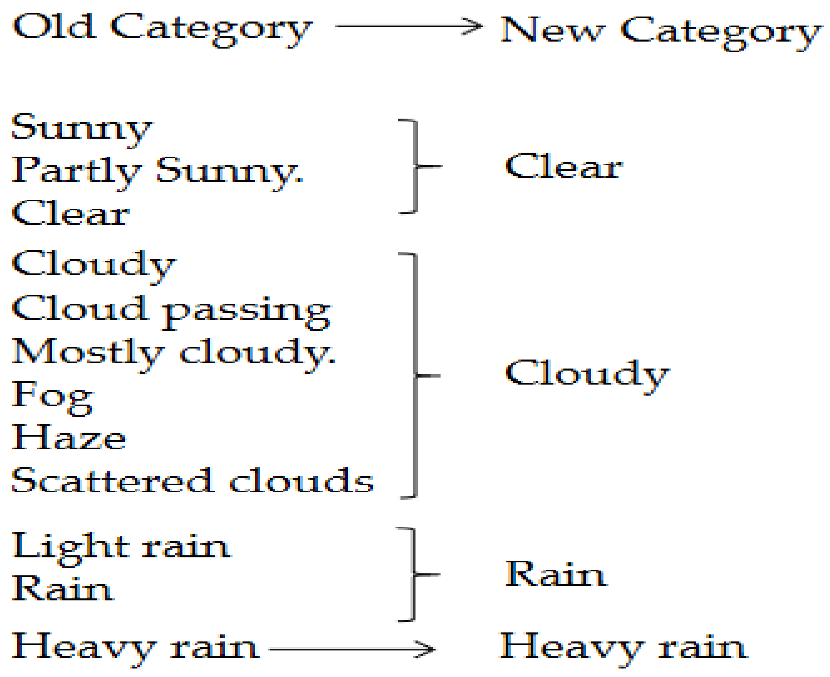
Besides the above external factors, weather conditions have a notable influence on taxi demands [2]. A weather dataset from 1 September 2013 to 30 November 2013 is also obtained by web data crawler tool from the timeanddate website [26]. For ease and simplification, weather categories are converted into categories defined as shown in Figure 3.
Moreover, the weather data includes other variables, including temperature, wind speed, humidity information, etc. To enhance weather data accuracy, we adopted updated data for every hour unless there is a change in the existing conditions.
4.2. Features Extraction and Analysis
To understand the detailed information behind taxi demands and significant correlated factors which play a vital role in taxi demands forecasting, we need to extract and analyze features from the raw multi-source data introduced in Section 4.1.
4.2.1. Taxi Trips
To enhance data accuracy and deal with invalid data such as incomplete, noisy data and outliers, etc. Raw GPS data have been manipulated and prepared carefully. The raw data have been explored using with outstanding packages and libraries in R language and Python such as Pandas, skit-learn and stats. Considering Wuhan graphical coordinates (longitude: 113°40′~115°04′ and latitude: 29°60~31°20′), the GPS records located outside this range deleted. Besides, GPS data with a taxi status of 0 or 2 (0: invalid device, 2: temporarily stopped) and repeated records were removed. GPS records of more than five sequential timestamps with zero speed value have been deleted.
In addition, data caused by the device errors and noises, such as GPS records with zero or null values of longitude, latitude, timestamp, were also deleted.
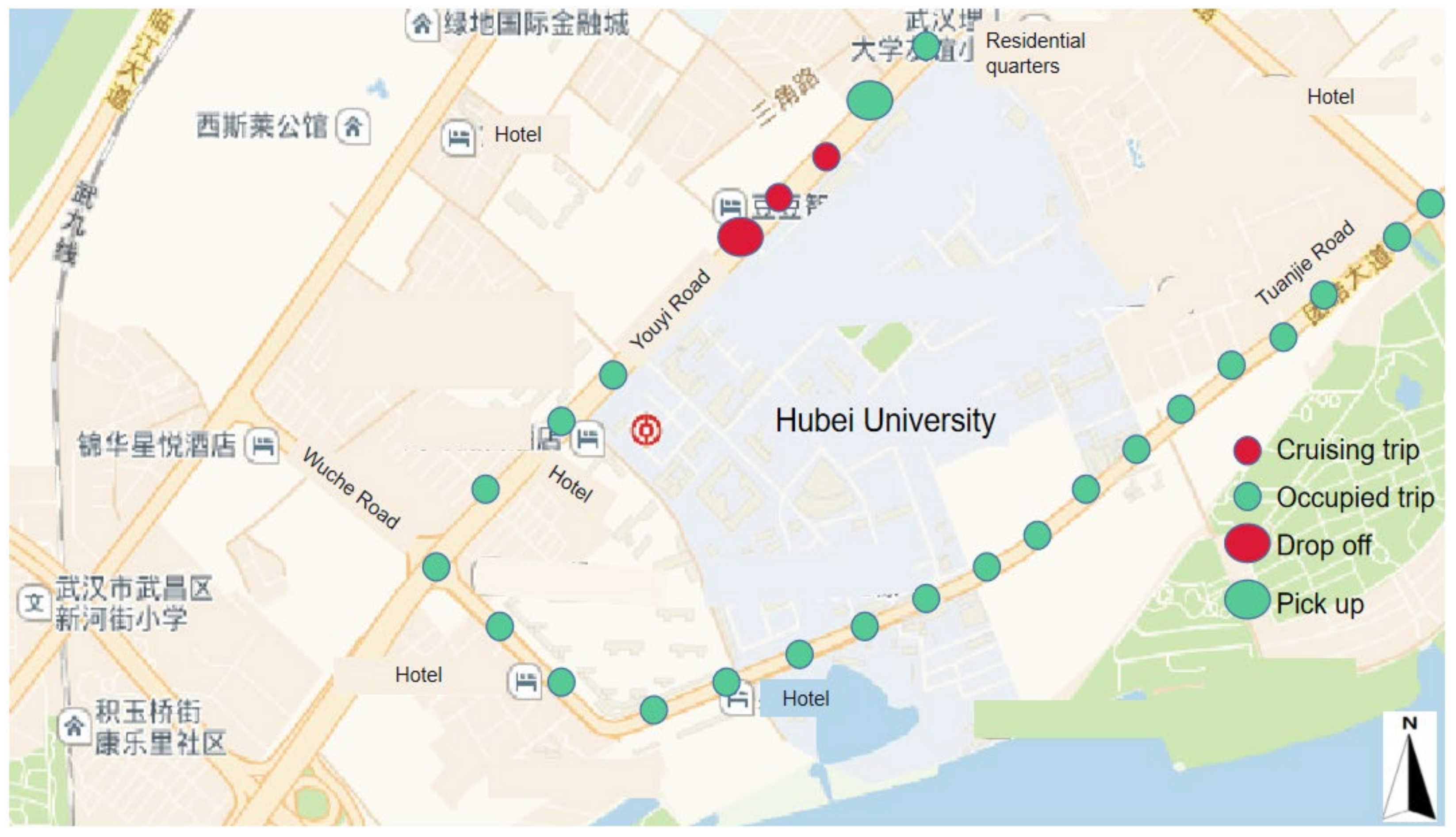
As in [27,28], taking into account taxi states during working operation, we can consider two trips: occupied (O) and vacant (V). The empty trip means that the taxi status value is 1, and the driver is cruising without a passenger, whereas in the occupied trip, the taxi is crossing the roads with a passenger. Figure 4 shows an example of the two trips randomly extracted from GPS trajectory taxi.
As shown in Figure 4, small green circles form an occupied trip with a giant green circle (represents a taxi pick up) and end up with a big red circle (represents a taxi drop off). In contrast, small red circles together are considered a vacant trip. In this study, taxi demand prediction focuses on occupied trips. Table 3 shows variables related to occupied trips.
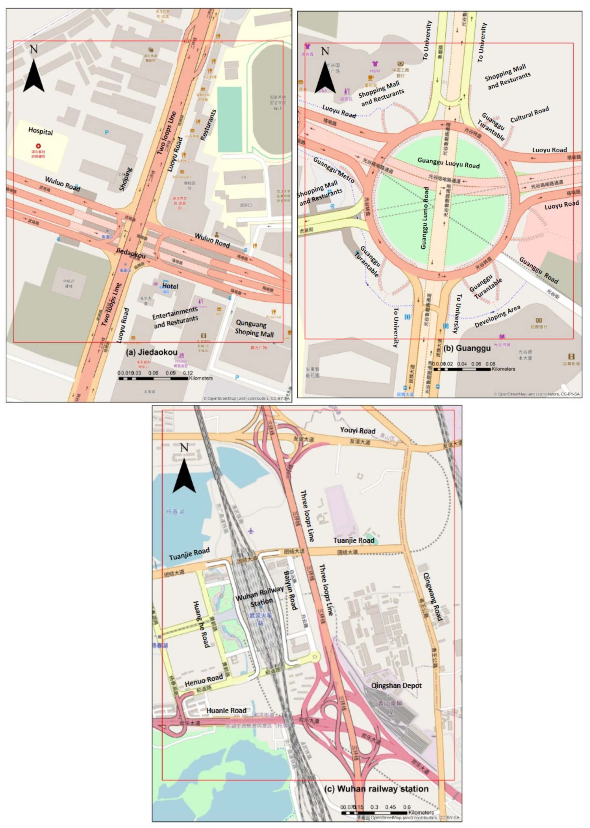
For the sake of more accurate results, the trips with a distance less than 200 m or trip period less than 3 min or number of GPS records less than five have been removed and are not considered in this study. Finally, the dataset considered 29,984,635 trips, and this number is sufficient for performing taxi demand prediction. Figure 5 shows three selected study areas in the city of Wuhan, (a) Jiedokou, (b) GuangGu area, and (c) Wuhan railway station area.
4.2.2. Taxi Demands and Temporal Factors
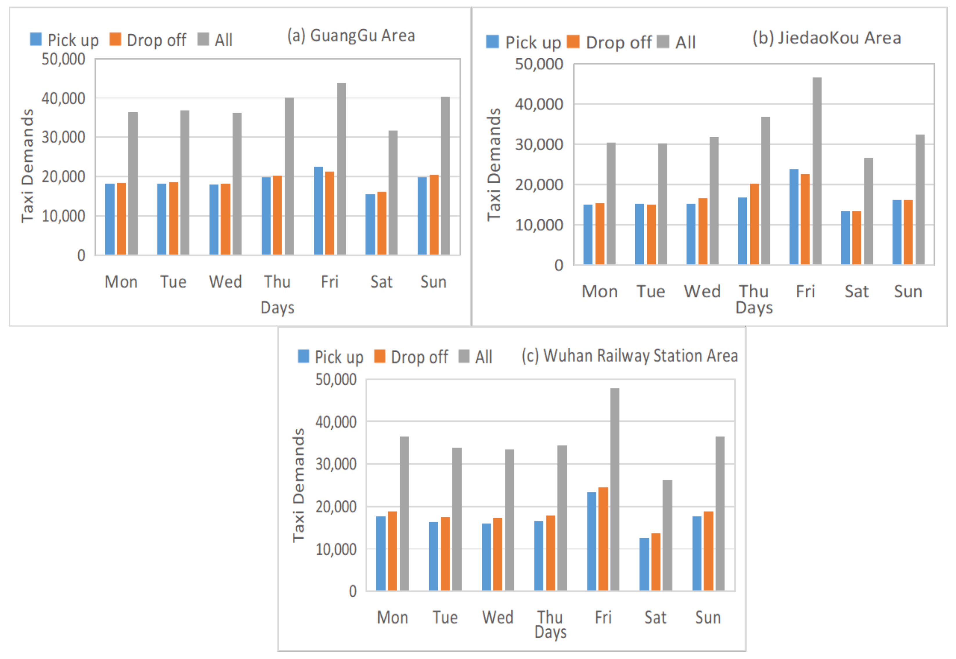
- Taxi demands distribution in Weekdays and Weekends
Figure 6 shows taxi demands distribution in Weekdays and Weekends of three study areas in the city of Wuhan.
We can see that these areas have similar taxi demand distributions (especially on Fridays, indicating that people take taxis on the last weekday for reasons such as going to travel or for entertainment or coming back on Sundays) and similar changes in taxi demands. Therefore, we can leverage the weekdays and weekends data to help in forecasting taxi demands.
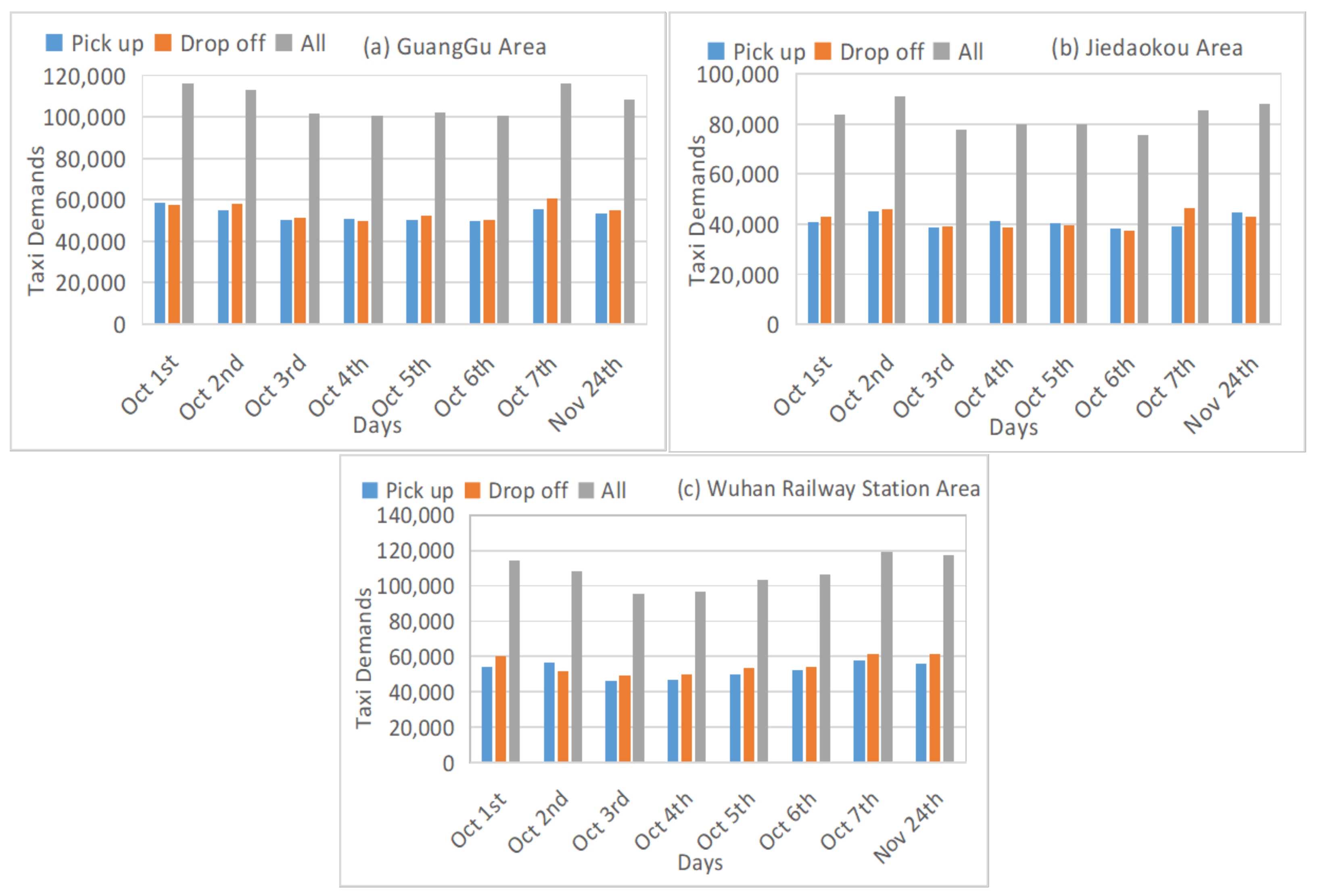
- Taxi demands distribution in Holidays
The collected dataset contains eight holidays (National days 1–7 October and 24 November Christmas day). Here we study the taxi demand distribution in the three study areas on the holidays, as shown in Figure 7.
In general, there is a noticeable pattern during holidays in the three areas. Days 1 and 2 October showed high taxi demands followed by a decrease in the other days and finally reached another high demand on7 October. It can be explained that in the beginning holiday period, and 24 November Christmas day, people may take taxis to travel. In contrast, taxi demands increase again on 7 October when people may come back home.
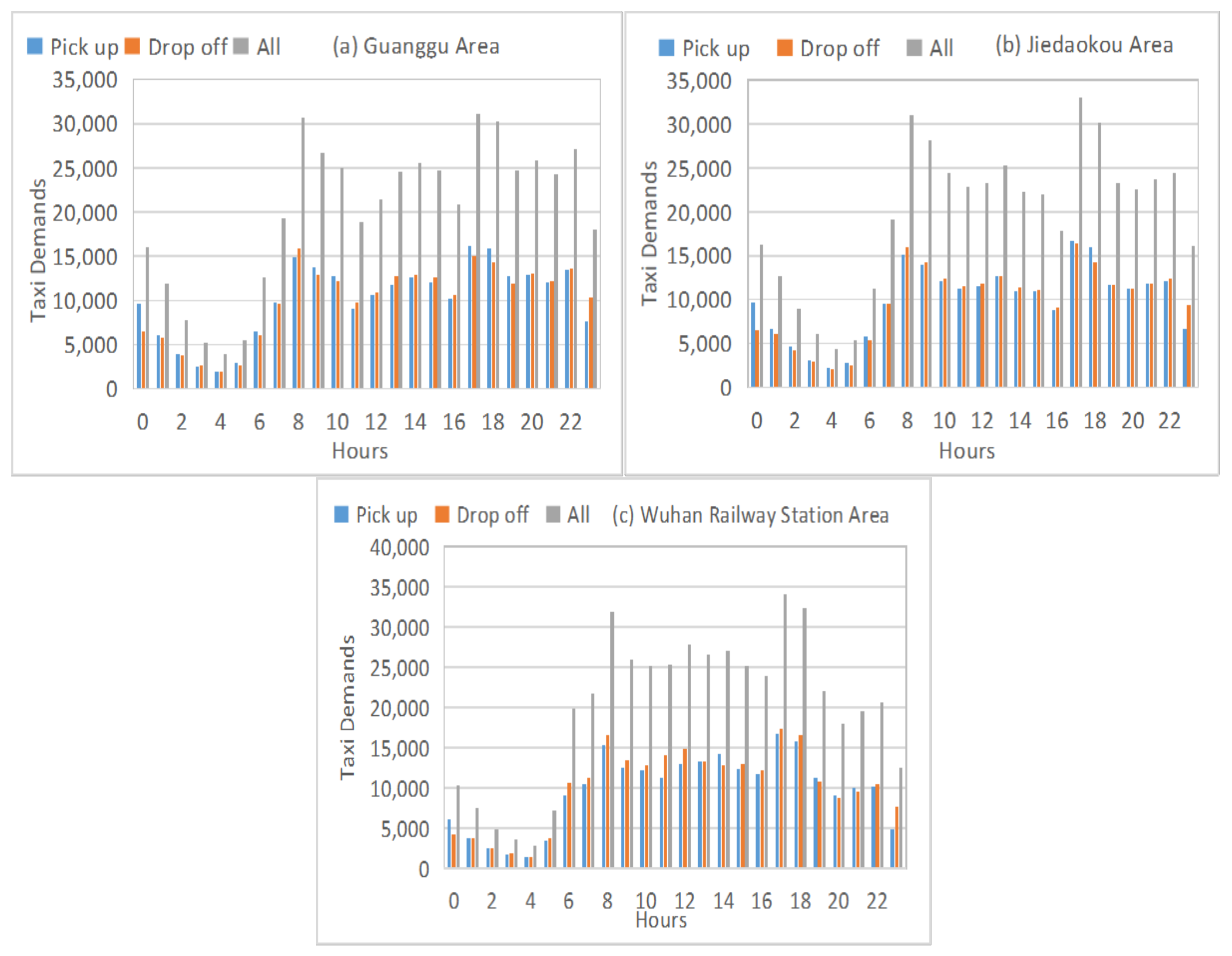
- Taxi demands distribution in daily hours
Figure 8 reports taxi demand distribution during a day (24 h) in the areas in Wuhan city.
As we can see in Figure 8, the three study areas have some shared patterns. For example, all of them showed the minimum rates at 4 am and peak-rush at 8 am and 5 pm.
The taxi demand shows high periodicity at long terms, due to the various changes of taxi demands on Thursdays and Fridays in many weeks are almost similar, in the three areas. The periodicity of short-term and long-term can assist in forecasting taxi demands in city areas in the future.
4.2.3. Taxi Demands and POI
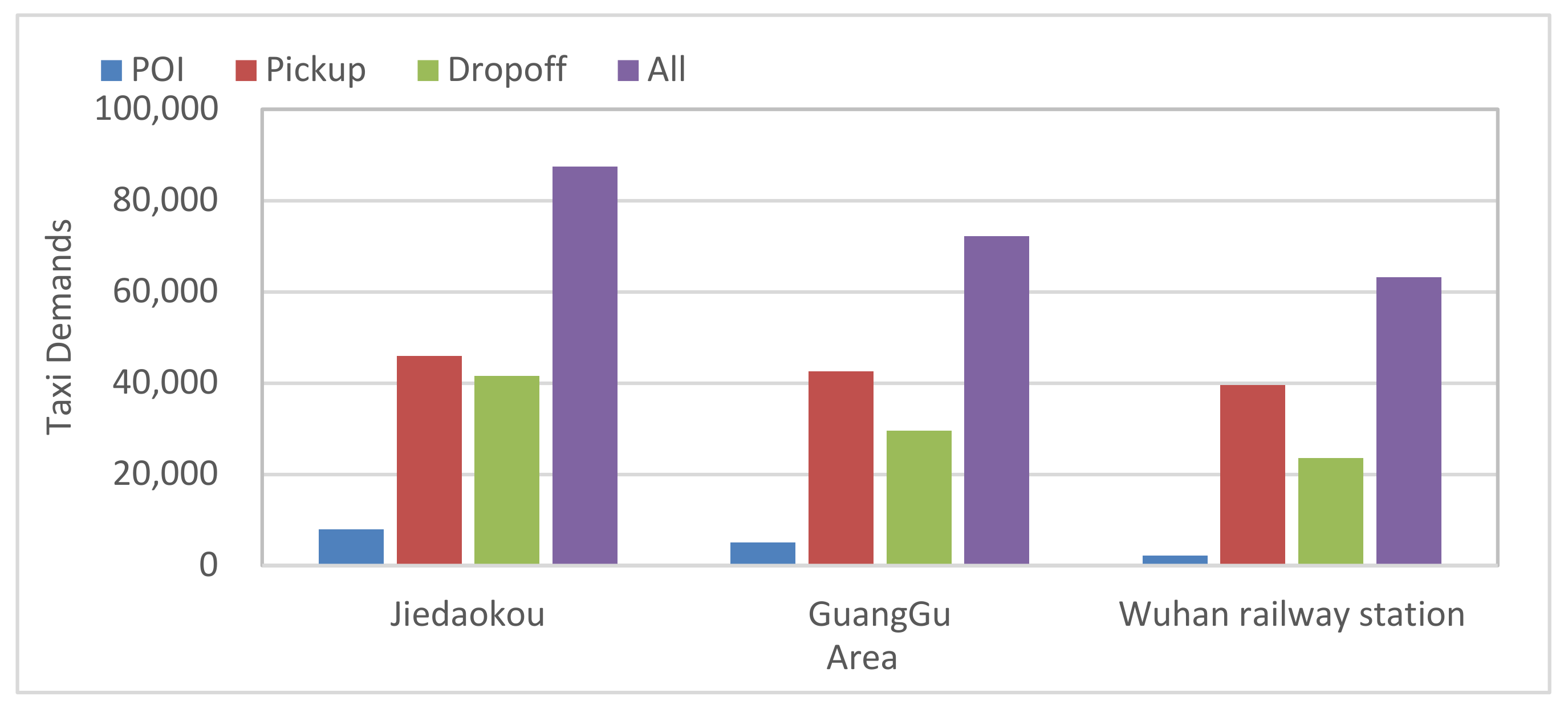
In general, the number and type POI may have a significant influence on taxi demand numbers. Figure 9 shows the distribution of POIs and taxi demands in the three areas of Wuhan city.
From Figure 9, we can find that the distribution of POIs and taxi demand is unbalanced over the three areas, and the more POIs there are in each area, the more taxi demands. For instance, POIs and taxi demands in Jiedaokou and Guanggu are at high numbers, while those in Wuhan railway are at lower numbers.
4.2.4. Taxi Demands and Weather Factors
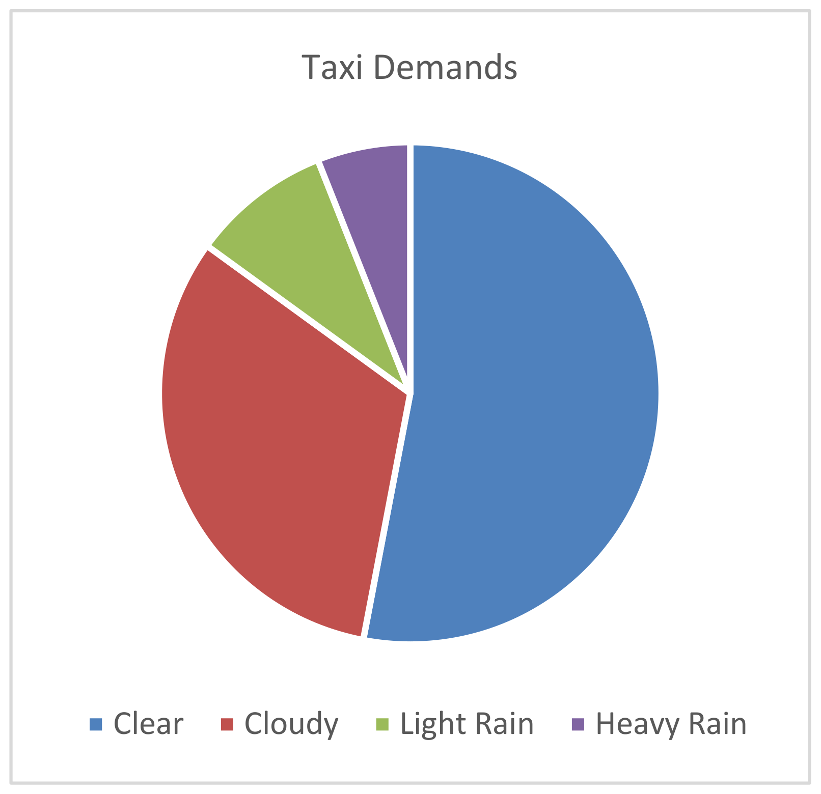
Besides the above factors, taxi demands are also influenced by weather conditions [22]. This study considers various weather-related factors, including weather conditions (e.g., fog, clear, and rainy), temperature, wind speed, and humidity information, etc., which are reported each hour. Figure 10 shows the general distribution by percentages of different weather types during the study periods.
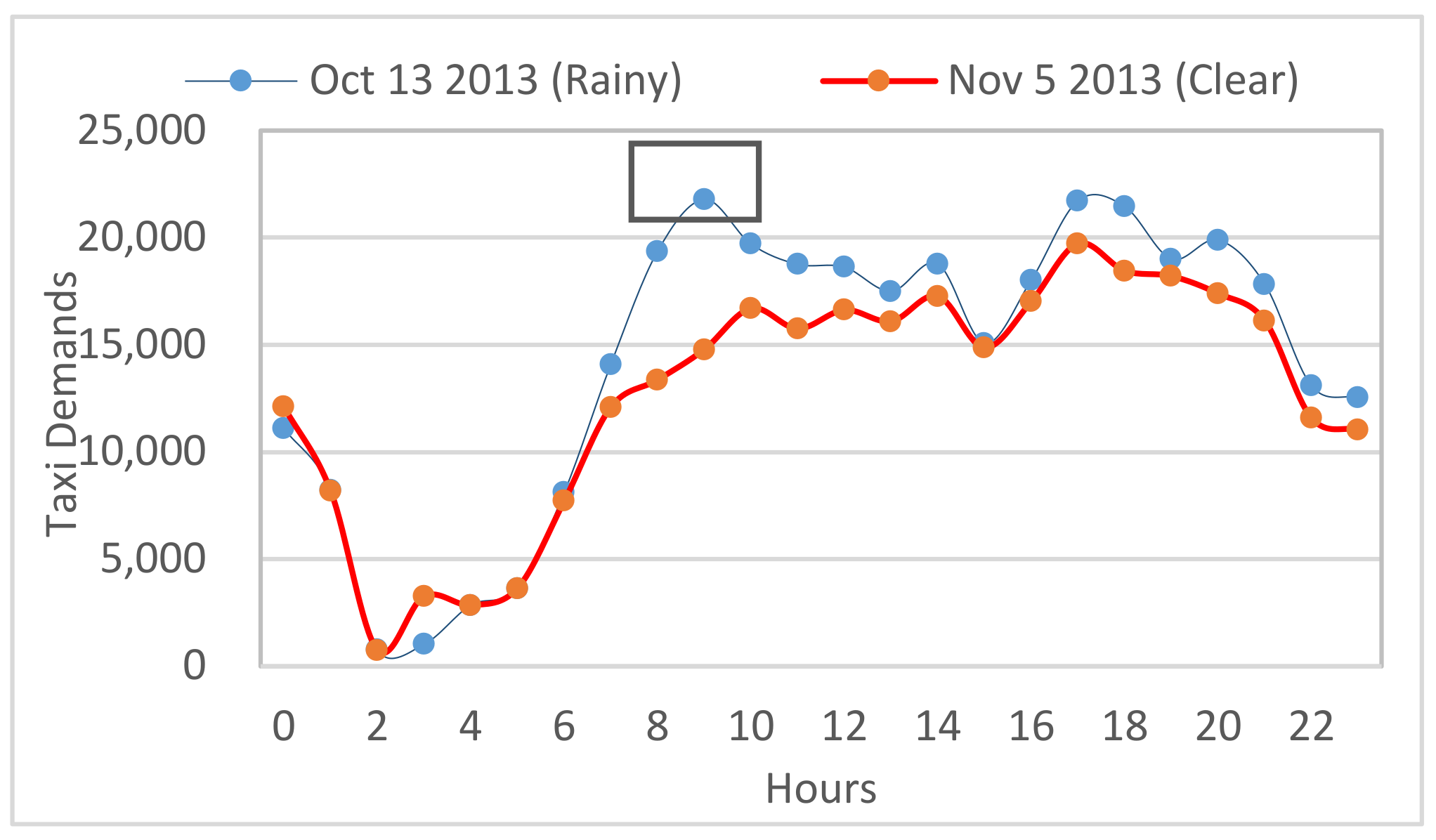
Figure 10 shows the general taxi demands of the three-study area in a day with various weather-related factors.
From Figure 11, we can observe a distinctly remarked impact of weather on taxi demands. We can find that taxi demands significantly increased on a rainy day, and more people may prefer to take taxis when it rains during 7–9 am. This can assist in providing information of taxi traffic flow and human traveling behavior. In adaption, with the functions of each area (using POI) we can understand the flow of passengers.
4.3. Features Preparation
After extracting and analyzing features and taxi demands, there is a need to prepare the features to be ready for utilization in the proposed model. Here we perform three steps: features normalization, transformation, and concatenation.
4.3.1. Feature Transformation
For the sake of reducing the complexity of computing factors, we transformed factors into categorical values, including: Is weekend, Is holiday, region, weather, etc. These factors’ values are converted to be numbers that begin with 0 and end with the summation number of the values. For instance, Is weekend factor’s values would be represented by 1 for a weekend and 0 for a weekday; weather condition’s value would be 0,1,2,3,4 for Clear, Cloudy, Rain, Light Rain, and Heavy Rain, respectively.
4.3.2. Feature Normalization
We use the Min-Max normalization [0, 1] standard to reduce the absolute scale’s effects. The normalization process is performed on continuous values as follows:
where x, xmin, xmax, xnorm are the original, minimum, maximum and normalized values from the dataset (training dataset), respectively.
4.3.3. Feature Concatenation
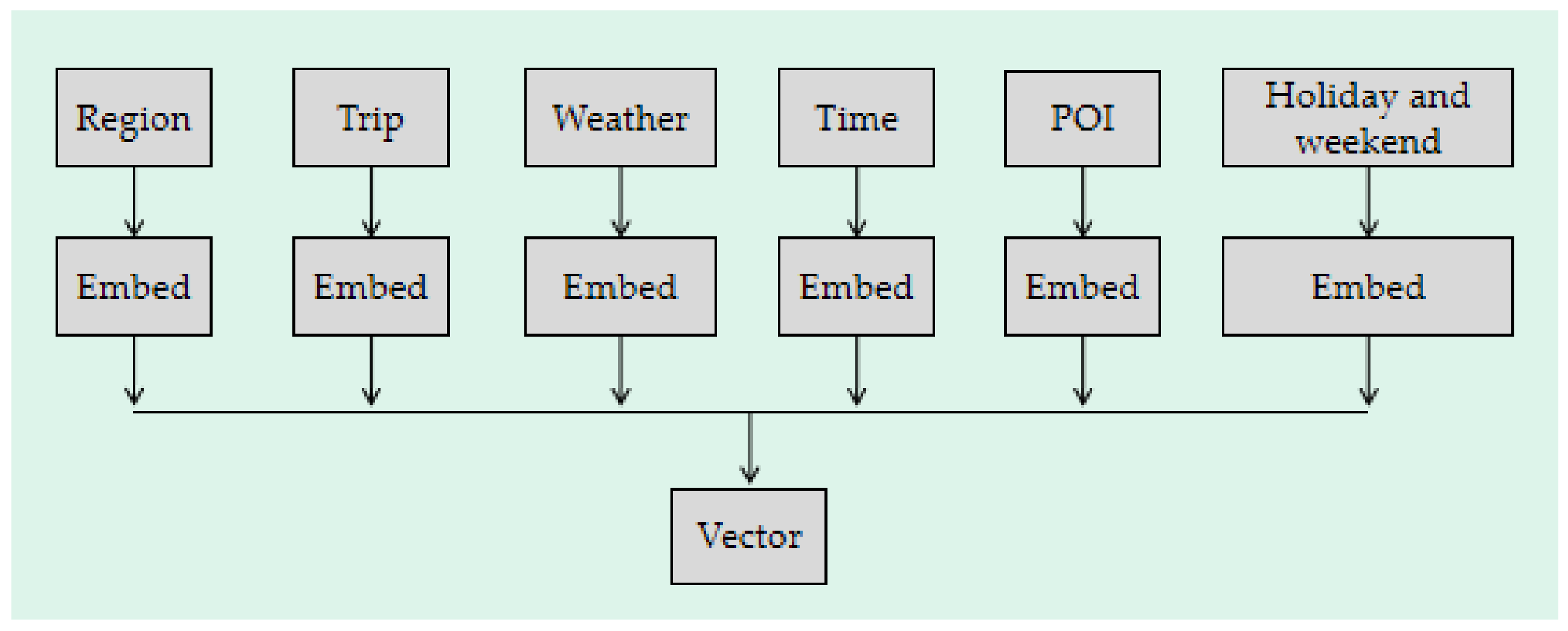
To facilitate the dataset training, we embed the features in Table 4 into a 1 × 11 vector according to a time-step t. Figure 12 depicts Feature Concatenation.
After performing features normalization, transformation, and concatenation, the dataset was ready for forecasting by prediction models. The features included in the dataset are shown in Table 4.
4.4. Generative Adversarial Network (GAN) Model
A generative adversarial network (GAN) contains two deep neural networks, a generator, and a discriminator. The generator network provides a (fake) dataset fed to the discriminator with the real data. The discriminator network determines and distinguishes the real data and the fake (generated) ones. During the model’s training process, both the generator and the discriminator’s weights would be updated using the related loss function. Once the discriminator becomes unable to differentiate the two types of data, it terminates the training process, and then the model becomes ready to be used; otherwise, in GANs, both components can be any deep neural network. In the following, we introduce LSTM andCNN and then illustrate the proposed GAN model used in this study.
4.4.1. LSTM and CNN
- LSTM
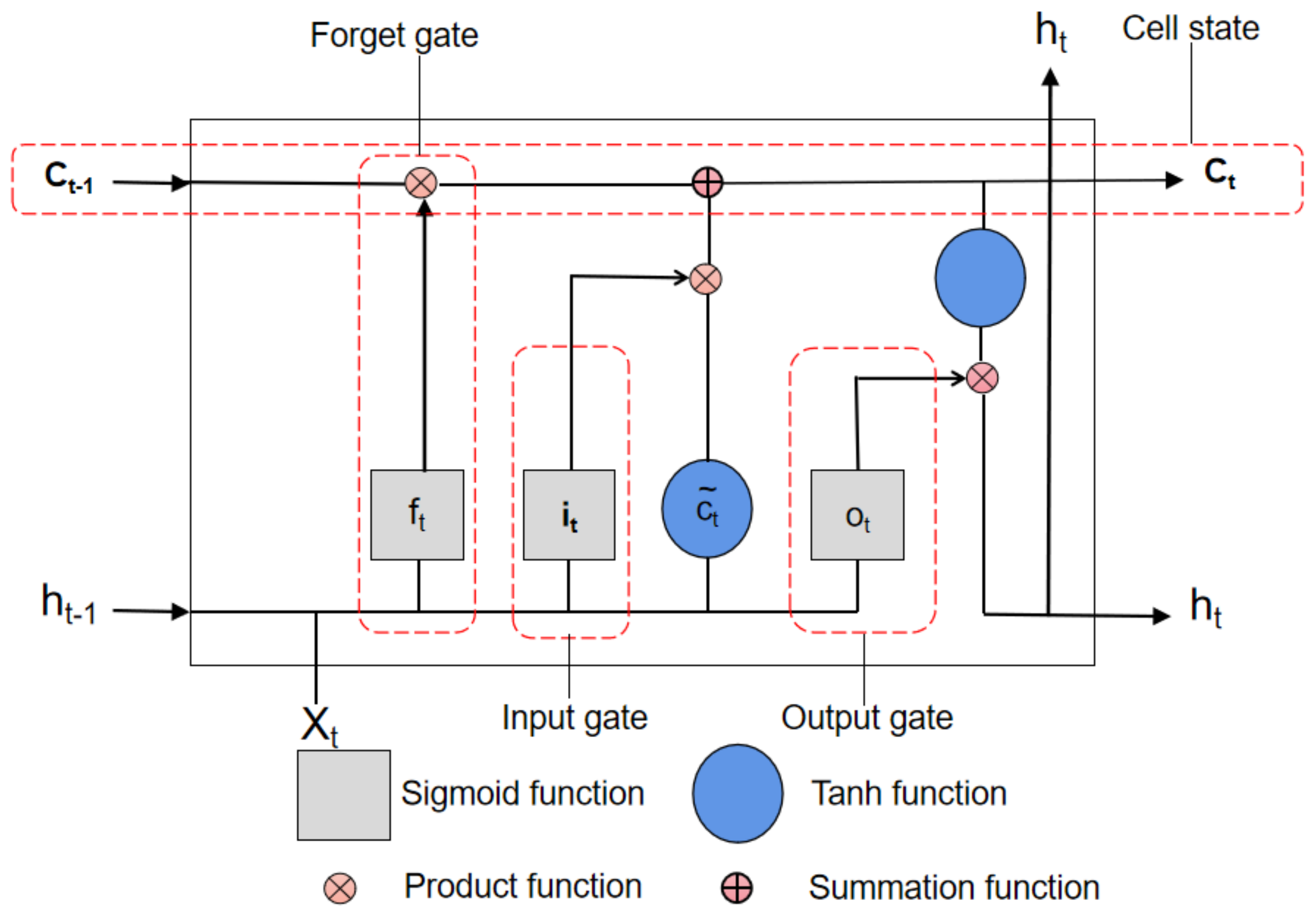
LSTM neural networks are emerged to add long-term memory function, which enhanced Recurrent Neural Networks’ ability to deal with more complicated issues, including prediction and classification [29]. In the LSTM network, the input vector sequence X would be mapped to an output vector sequence y by i iterations. Figure 13 depicts the architecture of an LSTM cell.
An LSTM cell contains three layers: an input layer, an output layer, and a memory block layer. The memory block includes three types of gates, including the input gate, the output gate ot, and the forget gate ft. Besides, ct and ct as memory cell vectors and the candidate value, respectively. The notation t represents a random time-step. During the training process, the related information can be updated as the following formula [30]:
where function is a sigmoid function can be computed as follows:
Wi, Wf, and Wc are the weight and the of the input gate, input gate, and input gate, respectively, whereas the function tanh(.) is a tangent function that is computed as follows:
- CNN
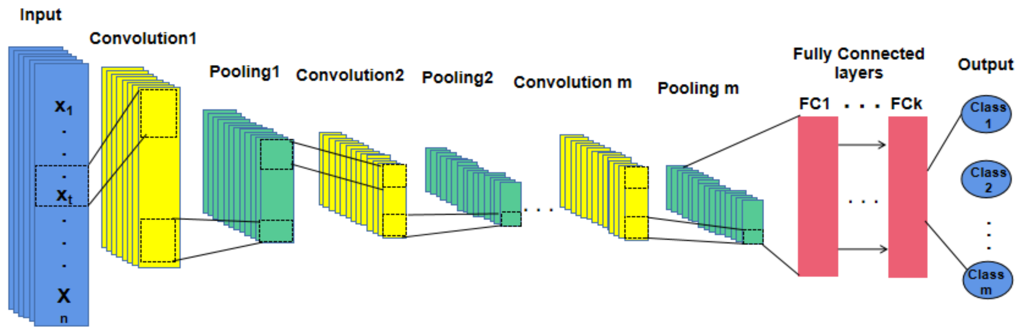
In general, Convolutional Neural Networks (CNNs) are composed of a convolutional cell group, pooling layers, and a set of fully connected layers, as depicted in Figure 14.
A convolutional layer i includes a group of filters Wi = ∈RS×D×N that is convolved with an input tensor, S denotes the filters’ number, D is a filter’s size, and N represents the input channels’ number [31]. A pooling layer can pool the output of a convolutional layer. Both convolutional and pooling layers are adopted to obtain the temporal patterns and to correlate temporally distant features. A set of fully connected layers follows the last convolutional/pooling layer to classify the input time series. The network output showed the dataset’s classification result and provided one of the two labels (real, predicted) for each time step.
4.4.2. GAN_LSTM_CNN Model
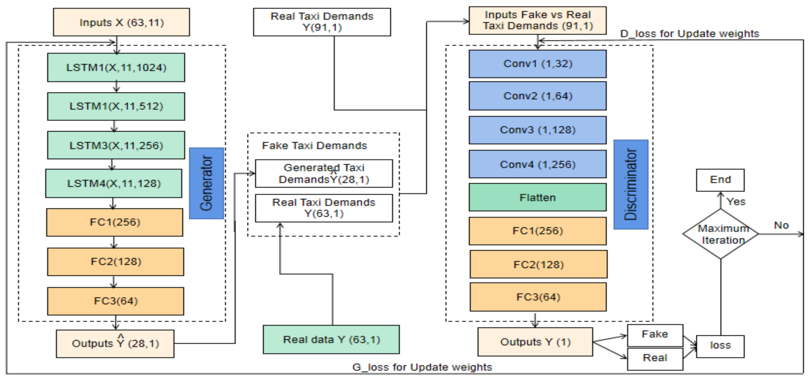
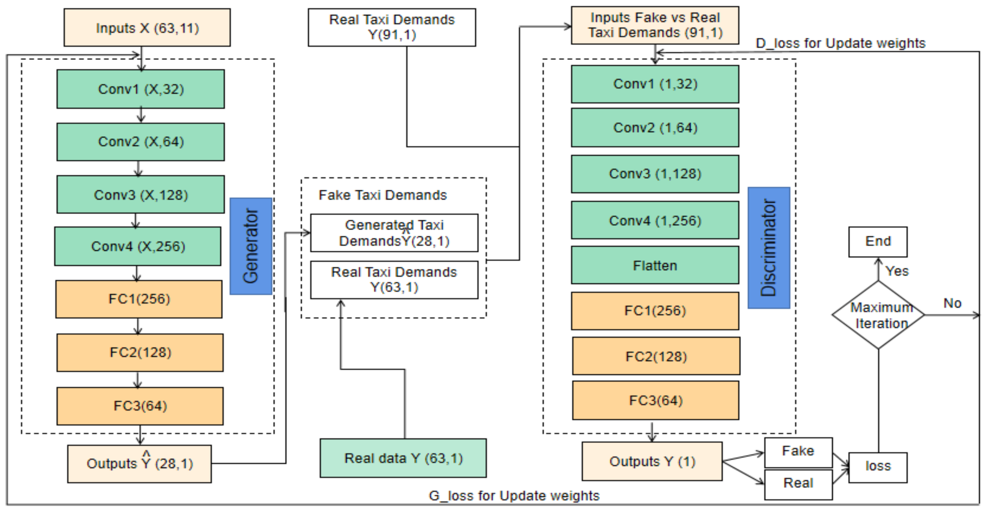
In the proposed model, and due to their stability, the generator component adopted LSTM networks and CNN for the discriminator network. Figure 15 illustrates the architecture of the GAN_LSTM_CNN Model.
- The generator
In our GAN model, we set the LSTM network as the generator according to its stability. The dataset contains 12 features (for 24 h of 91 days) as listed in Table 4. For building up a robust generator network with good performance, we use four layers of LSTM; the numbers of the neuron are 1024, 512, 256, and 128, followed by three fully connected layers. The activation function used in LSTMs is ReLU, and the dropout neurons are 20 percentage, and the neuron number of the latest layer will be the same as the output step we are going to predict.
- The discriminator
The discriminator in the proposed GAN model is a Convolutional Neural Network that aimed to distinguish whether the input data of the discriminator is real or fake. The input for the discriminator will be from the real data or the fake data from the generator. The discriminator network contains four Convolution layers with 32, 64, 128, and 256 neurons separately. Besides, a flatten layer is combined to flatten the output of the convolutional layers to generate a single feature vector for classification, which is performed by the following four fully connected layers with 220, 220,220, and a neuron, respectively. The Leaky Rectified Linear Unit (ReLU) has been set as the activation function on all layers, except the output layer (adopted Sigmoid function). The sigmoid function will produce a single scalar output, 0 or 1, which means real or fake as the final result.
4.4.3. Training Process
In the proposed model, the generator generates fake data and tries to fool the discriminator, whereas the discriminator tries to distinguish the real data from the predicted data. Thus, there is a need to perform dataset training on the generator and the discriminator. During the training process, the cross-entropy loss is utilized in our GAN model to minimize the difference between the two data distributions.
In training the discriminator, we aim to maximize its objective function, the probability of assigning the correct label to the samples, the loss function of the discriminator is defined as follows:
where x is the features vector, y is taxi demands from the real data, G(xi) is the generated taxi demands produced by the generator. Then we train the generator to minimize the loss function which is obtained as follows:
Through the training process, it always needs to minimize the loss function to obtain better results. In the proposed model, we adopted cross-entropy to calculate our loss for both generator and discriminator. In the discriminator, we combined the generated taxi demands with the historical taxi demands of input steps as our input for the discriminator. This step enhances the data length and increases the accuracy for the discriminator to learn the classification. In addition, the batch size is 30, and the epochs’ number is 400. We apply Leaky ReLU for fully connected layers as the activation Nesterov Accelerated Gradient (NAG) function. We utilized the NAG algorithm with a learning rate of 0.01 [31]. Besides, to avoid over-fitting, we implemented the dropout method with a probability of 0.2.
5. Experiment
This section introduces the experimental setting, baselines, evaluation metrics and shows the results of the proposed model and baselines in detail.
5.1. Experimental Settings
The main aim of this paper is to perform taxi demand prediction for the three-study areas in the city of Wuhan, including Jiedaokou, Guanggu, and Wuhan railway station, following 18 days with the data of the past 73 days (whole dataset 91 days in 24 h). During training the forecasting model, the input data contains not only the historical taxi demands but also 11 related features that might have a significant effect on the taxi demands. In the training process, the dataset will be split into a training dataset of 80% (73 days with 3264 observations) and a testing dataset of 20% (18 days with 649 observations).
Our model is implemented on a hardware environment of two GPUs, NVIDIA GeForce RTX 2070 with 32 Gigabyte memory, and executed by the conjunction of scikit-learn with the TensorFlow framework.
5.2. Model Comparison
To illustrate the effectiveness of our model, we compare the performance along with six mainstream baselines and tune the parameters for all methods. The models used for the comparison are as follows.
5.2.1. Auto-Regressive Integrated Moving Average (ARIMA)
In ARIMA (p,d,q), the parameters p and q are related to the order of the autoregressive term and the moving average term, respectively, while the parameter d indicates the dth order different from the original data series, which points to remove the trend from the data series [11]. In this study, these parameters were optimized by the auto-optimal function in the forecast functions in the sikit-learn package in python.
5.2.2. Gradient Boosting Decision Tree (XGBoost)
Researchers widely use XGBoost to perform traffic flow prediction and provide state-of-the-art results [32].
5.2.3. Multiple Layer Perceptron (MLP)
Our model is compared with the MLP method, which contains four hidden layers. The structure of every layer includes 128, 128, 128, and 64 hidden units, respectively.
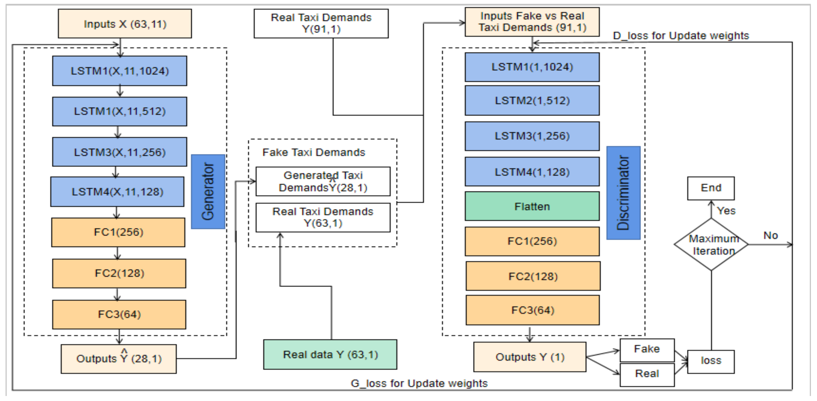
5.2.4. GAN_LSTM Model
In this model, both the generator and the discriminator have a similar structure as in the generative network G in the GAN_LSTM_CNN model, i.e., four LSTM layers and three fully connected layers. A flattening layer would be added as in the discriminator network in the GAN_LSTM_CNN model. Figure 16 shows the structure of the GAN_LSTM model.
5.2.5. GAN_CNN Model
In this model, the structure of the generator and discriminator is as same as the discriminator network D in the proposed GAN_LSTM_CNN model, i.e., four convolutional layers and three fully connected layers. Figure 17 represents the structure of the GAN_LSTM model.
5.3. Experimental Metrics
For the sake of assessing the verification and validation of a predictive model, many measures for assessing the predictive accuracy have been used [14,22]. Such as MAE, root MSE (RMSE) r and r2 are among the most commonly used or recommended measures [14,22,30]. Therefore, the commonly used measures, mean absolute error (MAE), root mean square error (RMSE), and the mean absolute percentage error, are considered in this study. The metrics are computed as the following formulas [29]:
where Yi,t is a real taxi demand in the area i at the time-step t, whereas is the predicted taxi demand. The constant number a in the Equation (15) is a small parameter (a = 1) to avoid division by zero situation when both Yi,t and are 0.
Thus, the forecasting performance by the three areas at time-step t can be defined as the followings:
By considering the initial batch size was 36, and the epoch size was 500, it was 50 iterations per epoch and totally about 25,000 iterations.
6. Results
6.1. Comparison with Baselines
This section illustrates a detailed comparison among models by experiential metrics as shown in Section 5.3. Firstly, we report the performance on MAE, sMAPE, and RMSE over the three areas together. Secondly, we show the prediction performance at the all specific areas as time passes, separately.
6.1.1. Performance Comparison over the Three Areas Together
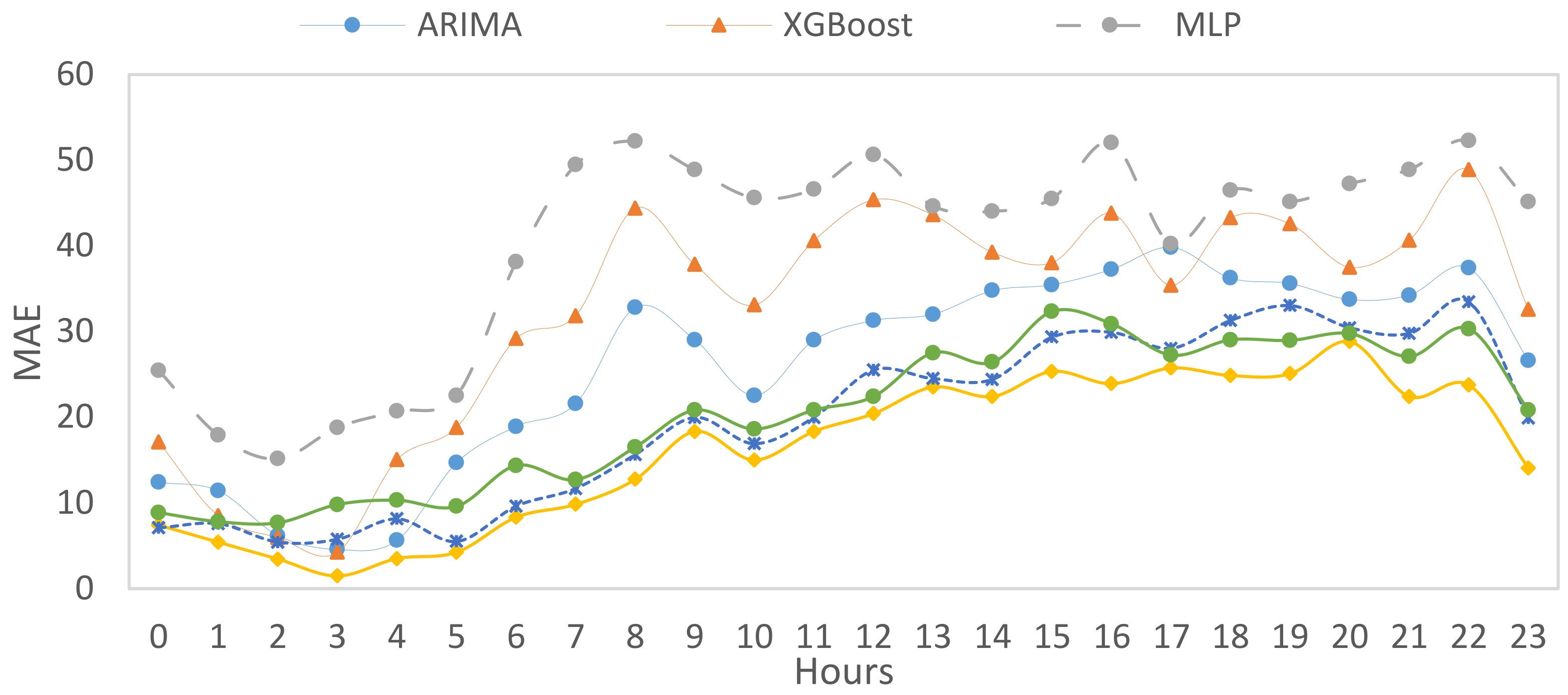
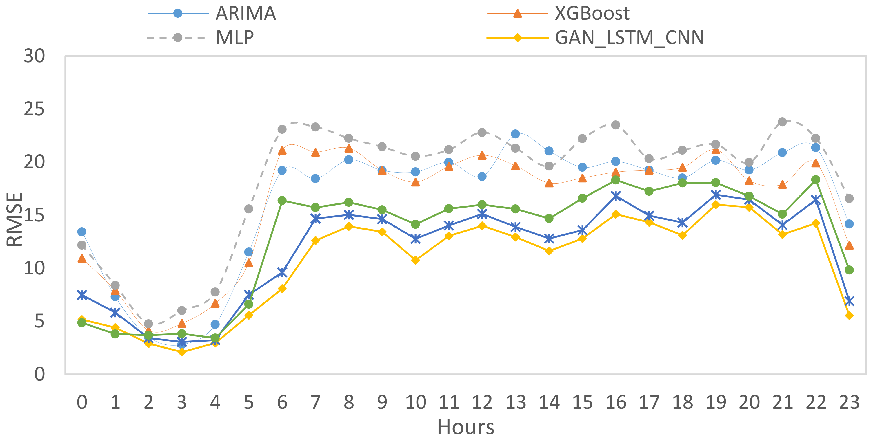
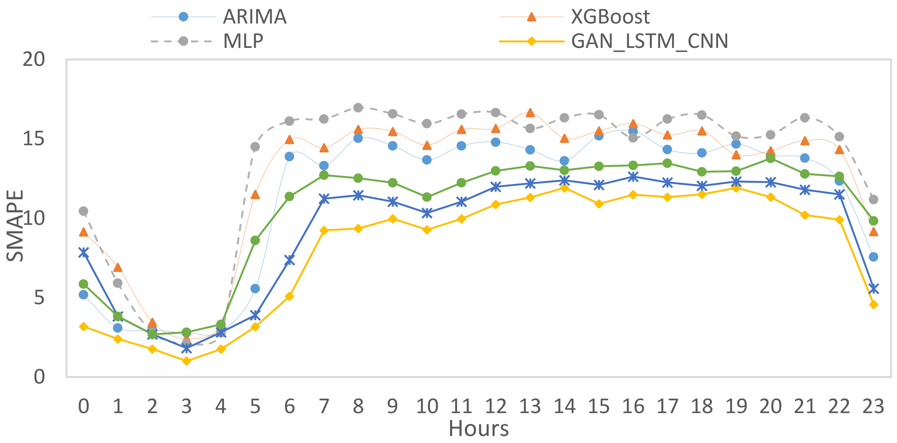
To assess the forecasting performance over the three study areas together (Jiedaokou area, Guanggu area, and Wuhan railway station area), we analyze the performance of the ARIMA, XBoost, MLP, GAN_LSTM_CNN model, GAN_LSTM, and GAN_CNN model in terms of MAE, RMSE, and sMAPE as defined in Equations (16)–(18). The comparison results are shown in Figure 18, Figure 19 and Figure 20.
From the three figures above, we can notice that although they are different forecasting performance metrics, there are some common patterns. For example, all metrics reach the minimum rates at three hours 3, 10, and 23 as the with lowest number of pickups wrt their neighboring time slots have. Moreover, the GAN_LSTM_CNN model presents a better performance compared to other predictors.
Figure 18 plots the mean absolute error (MAE), which describes the prediction accuracy. There is a dramatic decrease at the early hours of a day until it reaches 1.4 (the lowest point) in the GAN_LSTM_CNN model at 3 am, following with a gradual increase until 22, and then a further sharp fell is found.
As shown in Figure 19 and Figure 20, sMAPE presents the mean absolute error, whereas RMSE shows the root mean squared error between the predicted demands and the real demands. The values dropped from 3 am until 10 am, in which the value becomes lower again, then a noticeable increase has emerged again. GAN_LSTM_CNN model also provides the minimum MAPEs and RSMEs, which shows the highest accuracy between the predicted models adopted in this paper.
6.1.2. Performance Comparison over the Three Areas Separately
Our proposed model’s performance and the baselines for the three study areas, namely Jiedaokou, Wuhan Railway Station Area, and Guanggu, are shown in Table 5, Table 6 and Table 7.
As we can see from the three Tables above, we can notice that the GAN_LSTM_CNN model presents the lowest MAE, RMSE, and MAPE in the three areas, compared with the other baselines. Specifically, MLP and XGboost perform the poorest, whereas GAN_LSTM and GAN_CNN achieve good performance. Therefore, it proves that GAN-based models achieve better performance than other baselines. It confirms that deep neural networks can work efficiently in taxi demand forecasting. Compared withGAN_LSTM, GAN_LSTM_CNN model achieves 15.86% (2.31%, 13.46%) lower MAPE (RMSE, MAE) on Jiedaokou area, 9.22% (3.86%, 6.84%) lower MAPE (RMSE, MAE) on Wuhan railway Station area, and 4.69% (10.02%, 6.84) lower MAPE (RMSE, MAE) and on Guanggu area, respectively. Compared with GAN_CNN, our model reduced MAPE (RMSE, MAE) by 13.79% (4.77%, 12.29%) on the Jiedaokou area, 11.67% (11.45%, 9.93%) on Wuhan railway Station Area, and 4.38% (3.83%, 10.80%) on Guanggu area, respectively.
6.2. Comparison of Training Loss Function
The optimizer used in our model is the Adam algorithm with a learning rate of 0.0001. The batch size is 128, and we trained the model for 400 epochs. Figure 21 shows the Comparison of Training Loss Function among GAN_LSTM and GAN_CNN and GAN_LSTM_CNN models.
Figure 21a,b showed the loss of the GAN_LSTM and GAN_CNN. The blue line represents the loss path of the discriminator, and the orange line is the generator’s loss path. From the beginning, the loss of discriminator is higher than the loss of generator, and through the training process, both loss paths become flat.
In Figure 21c, the discriminator loss of GAN_LSTM_CNN decreases dramatically towards 0. Compared with GAN_LSTM and GAN_CNN, the discriminator in GAN_LSTM_CNN learns better and faster.
6.3. Comparison of Time Efficiency
We estimate the time efficiency reached by the GAN_LSTM_CNN model and GAN-based baselines (i.e., GAN_LSTM and GAN_CNN) in terms of the time consumption of training and testing.
As shown in Table 8, time spent for training and testing by GAN_LSTM is significantly larger than GAN_CNN and GAN_LSTM_CNN, even though its number of trainable parameters is the fewest. Moreover, we can found that our proposed GAN_LSTM_CNN achieves higher time consumption during training and testing processes than GAN_CNN. This is because the trainable parameters in GAN_LSTM_CNN are almost 22 times as much as in GAN_CNN.
7. Discussions
In this study, we try to investigate taxi demands and related factors extracted from multi-source data. A generative adversarial network (GAN) is adopted to forecast taxi-passenger demand by considering significant factors, including temporal, spatial, and external factors. Using GANs, the experiments showed that overall performance is very good compared to similar methods.
Comparing this study to the study by [2,5], we highlight several similarities and dissimilarities. Regarding their methodology and results, in particular, this study has several differences and innovations.
Firstly, a comprehensive experiment was conducted by GANs using multi-source data collected for the city of Wuhan in China, which covers all variables associated with taxi demand. The obtained variables include time, Is rush-time, Is weekend, Is holiday, Region, temperate, Weather, Wind, Humidity, and POI counts. In contrast, key variables were not included in the methods of Kuang Li et al.’s study [2] and Jun Xu et al.’s study [5], such as the POI counts, Is rush-time, Is weekend, Is holiday, Region, temperate, etc. These variables undoubtedly play a vital role in forecasting the taxi-passenger demand, and some of these variables were significant according to the results of this study. Not surprising that these factors are considered significant in forecasting taxi-passenger demand. It conforms to the findings of a previous study [16,18,29].
Secondly, Kuang Li et al.’s study [2] adopted the Convolutional Neural Network (CNN) to study contributing factors to taxi demand, but this study adopted a generative adversarial networks model. Three kinds of GANs have been adopted, namely the GAN_LSTM_CNN model, GAN_LSTM model, and GAN_CNN model. The results comparison indicated that the GAN_LSTM_CNN model outperformed the GAN_LSTM model and the GAN_CNN model in MAE, RMSE, and sMAPE introduced in Figure 18, Figure 19 and Figure 20. It shows that the GAN_LSTM_CNN model can present a more comprehensive view of the impact of significant factors on taxi demands.
Moreover, this study presents an analysis of the Training Loss Function among the GAN_LSTM_CNN model, GAN_LSTM model, and GAN_CNN model. It is important for considering computing consumed time during the Training process. The discriminator in GAN_LSTM_CNN shows that the model may learn better and faster, which can improve the efficiency and effectiveness of taxi demand prediction.
Finally, although the training time consumed by GAN_LSTM is considerably higher than those in GAN_CNN and GAN_LSTM_CNN, even though the trainable parameters are the lowest number. In addition, GAN_LSTM_CNN results in higher time consumption during training and testing processes than in GAN_CNN. This is reasonable as the training parameters in GAN_LSTM_CNN are 22 times bigger than those in GAN_CNN.
The findings of this study indicate that our hypothesis is correct. The results highlighted the vital role which deep learning-based methods can play in improving the accuracy of taxi demand forecasting. And this can help policy-makers regulating the taxi industry to enhance the temporal taxi supply during specific periods, which in turn can increase taxi profit.
Although the used dataset contains various vital variables, there are three limitations found during this study. The first is that more datasets can be collected for a more extended period, such as a year or two years. It may enhance the results and may provide a more accurate understating of taxi demands. The second limitation is the dataset used in this study is a historical dataset, not a real-time dataset. A real-time dataset may help in real-time traffic situations, where some areas have great demands and drivers compete for getting passengers in another area of the city. Thirdly, as the dataset of the whole city are huge, and beyond the capability of computers’ resources, we investigated three specific areas. If we have a considerable computer resource for dealing with such big data, a more comprehensive understanding of taxi demands would be obtained, which may help enhance taxi demands prediction.
8. Limitations
Although the used dataset contains various vital variables, there are three limitations found during this study. The first is that more datasets can be collected for a longer period such as a year or two years. This may enhance the results and may provide a more accurate understating of taxi demands. The second limitation is the dataset used in this study is a historical dataset, not a real-time dataset. Real-time dataset may help in real-time traffic situations, where some areas have large demands and drivers are competing with each other for getting passengers in another area of the city. Thirdly, as the dataset of the whole city are huge and beyond the capability of computers’ resources, we investigated three specific areas. If we have a huge computer resource for dealing with such big data, a more comprehensive understanding of taxi demands would be obtained which in turn may help in taxi demands prediction.
9. Conclusions
Accurate taxi demand forecasting can solve the traffic congestion problem caused by the supply-demand imbalance. Although many methods have been successfully employed to address the taxi demand prediction problem, most existing methods may not comprehensively consider various factors that influence the forecasting results. To fill the gap, we propose a deep learning-based model for forecasting taxi demands in the urban area by considering multi-source data.
Various factors have been considered, including trips factors, temporal factors, spatial factors, weather conditions, and POI. Firstly, in the proposed model, significant factors are extracted from raw data and then analyzed to understand the influences of these factors on taxi demands. Pick-up locations of Taxi trips are derived from taxi GPS trajectory, combined with temporal factors, weather conditions, POI data, and road network data. All information is then integrated to explore the travel pattern of taxi demand and its related influences.
Secondly, the extracted factors are prepared for use in the forecasting model. Normalization, transformation, and concatenation were employed. Thirdly, the Generative Adversarial Networks (GANs) structure is introduced, followed by a training process setting. The convolutional recurrent neural network model. In the proposed model, the LSTM network is adopted as the generator according to its stability. The convolutional neural network (CNN) is employed to distinguish whether the input data is real or generated by the generator. Finally, comprehensive experiments are performed on real-world datasets. The proposed model can automatically learn various characteristics to understand spatiotemporal patterns and enhance forecasting performance. For proving the xxx of predictive accuracy, the proposed model is validated and compared with several benchmark algorithms, including the ARIMA, XBoost, MLP, GAN_LSTM, and GAN_CNN on the real-world data of Wuhan city.
The results show that our model outperforms the other prediction approaches in the measurements of MAPE, RMSE, MAE, and time-consuming.
The evidence from findings proves that considering a deep learning-based approach and considering spatial-temporal, weather, road network correlations in models can significantly improve predictive accuracy. The results can assist policymakers in regulating the taxi industry to enhance the temporal taxi supply and the taxi lease rents (which vary by shift) for specific periods, which may improve passengers’ degree of satisfaction and improve the transportation capacities of the taxi industry cities.
For future work, there is a need to investigate the impact of other similar types of traffic demands such as online car-hailing services (for instance, didi and ober), which lead the taxi demands to be reduced. Moreover, the spatial correlation between city areas would be considered and then forecast taxi demand by graph-based deep neural networks.
Author Contributions
H.A.H.N. designed, developed the methodology, collected and analyzed the data; Q.X. supervised the work and provided analysis tools; H.A.H.N. wrote the paper; H.Z. performed data curation and visualization; T.L. project administration. All authors have read and agreed to the published version of the manuscript.
Funding
This study was supported by Foundation of Nanyang Institute of Technology (grant no.: 510102), Projects of Henan Provincial Department of Science and Technology (no. 212102310297).
Conflicts of Interest
The authors declare no conflict of interest.
References
- Bureau of Wuhan City’s Transportation. Analysis of Urban Passenger Transport Operation in Wuhan. 2021. Available online: http://jtj.wuhan.gov.cn/zwgk/zfxxgkml/tjsj/202102/t20210202_1624093.shtml (accessed on 21 August 2021).
- Kuang, L.; Yan, X.; Tan, X.; Li, S.; Yang, X. Predicting Taxi Demand Based on 3D Convolutional Neural Network and Multi-task Learning. Remote Sens. 2019, 11, 1265. [Google Scholar] [CrossRef] [Green Version]
- Qian, X.; Ukkusuri, S.V. Time-of-day pricing in taxi markets. IEEE Trans. Intell. Transp. Syst. 2017, 18, 1610–1622. [Google Scholar] [CrossRef]
- Le Quy, T.; Nejdl, W.; Spiliopoulou, M.; Ntoutsi, E. In A neighborhood-augmented LSTM model for taxi-passenger demand prediction. In International Workshop on Multiple-Aspect Analysis of Semantic Trajectories; Springer: Cham, Switzerland, 2019; pp. 100–116. [Google Scholar]
- Xu, J.; Rahmatizadeh, R.; Boloni, L.; Turgut, D. Real-Time Prediction of Taxi Demand Using Recurrent Neural Networks. IEEE Trans. Intell. Transp. Syst. 2017, 19, 1–10. [Google Scholar] [CrossRef]
- Niu, K.; Cheng, C.; Chang, J.; Zhang, H.; Zhou, T. Real-Time Taxi-Passenger Prediction With L-CNN. IEEE Trans. Veh. Technol. 2019, 68, 4122–4129. [Google Scholar] [CrossRef]
- Tang, J.; Liang, J.; Zhang, S.; Huang, H.; Liu, F. Inferring driving trajectories based on probabilistic model from large scale taxi GPS data. Phys. A Stat. Mech. Appl. 2018, 506, 566–577. [Google Scholar] [CrossRef]
- Moreira-Matias, L.; Gama, J.; Ferreira, M.; Damas, L. A predictive model for the passenger demand on a taxi network. In Proceedings of the 15th International IEEE Conference on Intelligent Transportation Systems, Anchorage, AK, USA, 16–19 September 2012; pp. 1014–1019. [Google Scholar]
- Liu, Z.; Chen, H.; Li, Y.; Zhang, Q. Taxi Demand Prediction Based on a Combination Forecasting Model in Hotspots. J. Adv. Transp. 2020, 2020, 1–13. [Google Scholar] [CrossRef]
- Chang, H.-W.; Tai, Y.-C.; Hsu, J.Y.-J. Context-aware taxi demand hotspots prediction. Int. J. Bus. Intell. Data Min. 2010, 5, 3–18. [Google Scholar] [CrossRef]
- Jamil, M.S.; Akbar, S. Taxi passenger hotspot prediction using automatic ARIMA model. In Proceedings of the 2017 3rd International Conference on Science in Information Technology (ICSITech), Bandung, Indonesia, 25–26 October 2017; pp. 23–28. [Google Scholar]
- Li, X.; Pan, G.; Wu, Z.; Qi, G.; Li, S.; Zhang, D.; Zhang, W.; Wang, Z. Prediction of urban human mobility using large-scale taxi traces and its applications. Front. Comput. Sci. 2012, 6, 111–121. [Google Scholar]
- Zhang, L.; Chen, C.; Wang, Y.; Guan, X. Exploiting taxi demand hotspots based on vehicular big data analytics. In Proceedings of the 2016 IEEE 84th Vehicular Technology Conference (VTC-Fall), Montreal, QC, Canada, 18–21 September 2016; pp. 1–5. [Google Scholar]
- Markou, I.; Rodrigues, F.; Pereira, F.C. Real-Time Taxi Demand Prediction using data from the web. In Proceedings of the 2018 21st International Conference on Intelligent Transportation Systems (ITSC), Maui, HI, USA, 4–7 November 2018; pp. 1664–1671. [Google Scholar]
- Liu, Z.; Chen, H.; Sun, X.; Chen, H. Data-driven real-time online taxi-hailing demand forecasting based on machine learning method. Appl. Sci. 2020, 10, 6681. [Google Scholar] [CrossRef]
- Saadi, I.; Wong, M.; Farooq, B.; Teller, J.; Cools, M. An investigation into machine learning approaches for forecasting spatio-temporal demand in ride-hailing service. arXiv 2017, arXiv:1703.02433. [Google Scholar]
- Ma, X.; Yu, H.; Wang, Y.; Wang, Y. Large-scale transportation network congestion evolution prediction using deep learning theory. PLoS ONE 2015, 10, e0119044. [Google Scholar] [CrossRef] [PubMed]
- Zhang, J.; Zheng, Y.; Qi, D.; Li, R.; Yi, X. DNN-based prediction model for spatio-temporal data. In Proceedings of the 24th ACM SIGSPATIAL International Conference on Advances in Geographic Information Systems, Burlingame CA, USA, 31 October–3 November 2016; pp. 1–4. [Google Scholar]
- Rossi, A.; Barlacchi, G.; Bianchini, M.; Lepri, B. Modelling taxi drivers’ behaviour for the next destination prediction. IEEE Trans. Intell. Transp. Syst. 2019, 21, 2980–2989. [Google Scholar] [CrossRef]
- Zhao, Z.; Chen, W.; Wu, X.; Chen, P.C.; Liu, J. LSTM network: A deep learning approach for short-term traffic forecast. IEEE Trans. Intell. Transp. Syst. 2017, 11, 68–75. [Google Scholar] [CrossRef] [Green Version]
- Ke, J.; Zheng, H.; Yang, H.; Chen, X. Short-term forecasting of passenger demand under on-demand ride services: A spatio-temporal deep learning approach. Transp. Res. Part C Emerg. Technol. 2017, 85, 591–608. [Google Scholar] [CrossRef] [Green Version]
- Liu, T.; Wu, W.; Zhu, Y.; Tong, W. Predicting taxi demands via an attention-based convolutional recurrent neural network. J. Knowl.-Based Syst. 2020, 206, 106294. [Google Scholar] [CrossRef]
- Zhang, J.; Zheng, Y.; Qi, D. Deep spatio-temporal residual networks for citywide crowd flows prediction. In Proceedings of the AAAI Conference on Artificial Intelligence, San Francisco, CA, USA, 4–9 February 2017. [Google Scholar]
- OpenStreetMap. Available online: https://www.openstreetmap.org/ (accessed on 17 March 2021).
- Guihuayun. Available online: http://www.guihuayun.com/ (accessed on 5 November 2020).
- Timeanddate. Available online: https://www.timeanddate.com/ (accessed on 10 November 2020).
- Hasan, N.; Wu, C.; Hui, Z. Understanding the Impact of Human Mobility Patterns on Taxi Drivers’ Profitability Using Clustering Techniques: A Case Study in Wuhan, China. Information 2017, 8, 67. [Google Scholar]
- Naji, H.; Wu, C.; Hui, Z.; Li, L. Towards understanding the impact of human mobility patterns on taxi drivers’ income based on GPS data: A case study in Wuhan—China. In Proceedings of the 2017 4th International Conference on Transportation Information and Safety (ICTIS), Banff, AB, Canada, 8–10 August 2017. [Google Scholar]
- Yu, H.; Chen, X.; Li, Z.; Zhang, G.; Liu, P.; Yang, J.; Yang, Y. Taxi-based mobility demand formulation and prediction using conditional generative adversarial network-driven learning approaches. IEEE Trans. Intell. Transp. Syst. 2019, 20, 3888–3899. [Google Scholar] [CrossRef]
- Bogaerts, T.; Masegosa, A.D.; Angarita-Zapata, J.S.; Onieva, E.; Hellinckx, P. A graph CNN-LSTM neural network for short and long-term traffic forecasting based on trajectory data. Transp. Res. Part C Emerg. Technol. 2020, 112, 62–77. [Google Scholar] [CrossRef]
- Lv, J.; Li, Q.; Sun, Q.; Wang, X. T-CONV: A Convolutional Neural Network for Multi-scale Taxi Trajectory Prediction. In Proceedings of the 2018 IEEE International Conference on Big Data and Smart Computing (BigComp), Shanghai, China, 15–18 January 2018. [Google Scholar]
- Vanichrujee, U.; Horanont, T.; Pattara-Atikom, W.; Theeramunkong, T.; Shinozaki, T. Taxi Demand Prediction using Ensemble Model Based on RNNs and XGBOOST. In Proceedings of the 2018 International Conference on Embedded Systems and Intelligent Technology & International Conference on Information and Communication Technology for Embedded Systems (ICESIT-ICICTES), Khon Kaen, Thailand, 7–9 May 2018; pp. 1–6. [Google Scholar]
Figure 1.
Framework of the proposed model.

Figure 2.
(a) Road network, (b) Main regions of the city of Wuhan.

Figure 3.
Weather categories from historical Weather data.

Figure 4.
An example of the two trips randomly extracted from a GPS taxi trajectory. The occupied trip crossed Tuanjie road and ends at the gate of Hubei university and dropped off the passenger, and after several meters another passenger is picked up and anther occupied trip begins.
Figure 4.
An example of the two trips randomly extracted from a GPS taxi trajectory. The occupied trip crossed Tuanjie road and ends at the gate of Hubei university and dropped off the passenger, and after several meters another passenger is picked up and anther occupied trip begins.

Figure 5.
Three study areas in the city of Wuhan, (a) Jiedaokou area, (b) Guanggu area, (c) Wuhan railway station area.
Figure 5.
Three study areas in the city of Wuhan, (a) Jiedaokou area, (b) Guanggu area, (c) Wuhan railway station area.

Figure 6.
Taxi demands distribution in Weekdays and Weekends in the city of Wuhan. Weekday show high taxi demands as they related to working time, Sunday has a high number of Taxi demands as well.
Figure 6.
Taxi demands distribution in Weekdays and Weekends in the city of Wuhan. Weekday show high taxi demands as they related to working time, Sunday has a high number of Taxi demands as well.

Figure 7.
Taxi demands distribution in the city of Wuhan during holidays. Holidays show high taxi demands in the three areas.
Figure 7.
Taxi demands distribution in the city of Wuhan during holidays. Holidays show high taxi demands in the three areas.

Figure 8.
Taxi demands distribution in the city of Wuhan during daily hours.

Figure 9.
Distribution of POIs and taxi demands in different regions.

Figure 10.
General distribution by percentages of different weather types.

Figure 11.
Weather Influence on Taxi demands.

Figure 12.
Feature Concatenation.

Figure 13.
The architecture of a traditional LSTM network.

Figure 14.
The architecture of traditional Convolutional Neural Network.

Figure 15.
The architecture of GAN_LSTM_CNN model.

Figure 16.
The structure of GAN_LSTM model.

Figure 17.
The structure of GAN_CNN model.

Figure 18.
MAE Comparison Results with different time slots. MLP, XGBoost attained high MAE whereas GAN_LSTM_CNN achieved better MAE.
Figure 18.
MAE Comparison Results with different time slots. MLP, XGBoost attained high MAE whereas GAN_LSTM_CNN achieved better MAE.

Figure 19.
RMSE Comparison Results with hours ranged from 0–23 with increasing values from 6:00 to 22:00 and all deep learning methods achieved better results.
Figure 19.
RMSE Comparison Results with hours ranged from 0–23 with increasing values from 6:00 to 22:00 and all deep learning methods achieved better results.

Figure 20.
sMAPE Comparison Results during time slots. The achieved values showed deep learning methods (such as GAN_CNN, GAN_LSTM, GAN_LSTM_CNN) achieved better results comparing to ARIMA, XGBoost an MLP.
Figure 20.
sMAPE Comparison Results during time slots. The achieved values showed deep learning methods (such as GAN_CNN, GAN_LSTM, GAN_LSTM_CNN) achieved better results comparing to ARIMA, XGBoost an MLP.

Figure 21.
Training loss of the Generator(G_loss) and Discriminator(D_loss) of (a) GAN_LSTM, (b) GAN_CNN and (c) GAN_LSTM_CNN models. In GAN_LSTM and GAN_CNN, the loss of discriminator is higher than the loss of generator, and through the training process, both loss paths become flat. Compared with GAN_LSTM and GAN_CNN, the discriminator in GAN_LSTM_CNN learns better and faster.


Table 1.
Description of the attributes of a record in the Taxi GPS dataset.
| Attribute | Description | Example |
|---|---|---|
| Taxi (Driver) ID | 8~10 digit number as taxi identifier. | 28784651 |
| Time | 14-digit number, format yyyyMMddHHmmss | 20131112181211 |
| Longitude | 2~3 digit number with 6 decimals, in the degree unit. | 33.2260002 |
| Latitude | 2~3 digit number with 6 decimals, in the degree unit. | 114.232253 |
| Speed | Taxi speed in miles/hour unit. | 39.57 |
| Taxi Status | 0: Taxi device is invalid, 1: Taxi not occupied; 2: temporarily stopped, 3: occupied. | 0,1,2,3 |
| Direction | 2~3 digit number with 2 decimals, in the degree unit. | 141.71 |
Table 2.
Description of POIs categories in the city of Wuhan.
| Category | Total Number | Description |
|---|---|---|
| C1 | 20034 | Transportation locations and related services |
| C2 | 8358 | Accommodation and related services such as hotels. |
| C3 | 9902 | Sports |
| C4 | 3402 | Public facilities and public toilets |
| C5 | 44160 | Business and Companies |
| C6 | 10846 | Health and beauty |
| C7 | 12013 | Government and Community |
| C8 | 17450 | Business residence; residential district |
| C9 | 19432 | Education |
| C10 | 63608 | Life activities and Entertainment |
| C11 | 121239 | Shopping |
| C12 | 1357 | Scenic Attraction and Travel |
| C13 | 62922 | Food and Dining |
Table 3.
Attributes of an occupied trip.
| Attribute | Description |
|---|---|
| Occupied trip ID | represents Taxi ID and trip number such as 28784651_10 |
| Pick up time-stamp | Format 20131112181211 represents year, month, date and time. |
| Pick up coordinates | includes longitude, latitude of a pick up event. |
| Drop off time-stamp | Format 20131112181211 represents year, month, date and time. |
| Drop off coordinates | includes longitude, latitude of a drop off event. |
| Occupied trip distance | Distance by kilometers |
| Occupied trip period | Period by minutes |
| GPS Record number | The number of GPS records in an occupied trip. |
Table 4.
Features in the dataset.
| Factor | Symbol | Data-Type | Description |
|---|---|---|---|
| Output (y) | |||
| Taxi demands | dems | continuous | Summation of Taxi pickups and dropoffs |
| Inputs (x) | |||
| Date | dt | time series | Date Format month-date |
| Time | tm | time series | Time Format hour:mints |
| Is rush-time | rush | categorical | 1. Yes 0. No |
| Is weekend | weekend | categorical | 1. Yes 0. No |
| Is holiday | holiday | categorical | 1. Yes 0. No |
| Region | reg | categorical | Determining region by longitude and latitude |
| Temperature | temp | continuous | Temperature |
| Weather | weath | categorical | 0. Clear 1. Light Rain 2. Heavy Rain 3. Fog |
| Wind | wind | continuous | Wind (km\h) |
| Humidity | humid | continuous | Humidity by percentage |
| poi_counts | poi | continuous | POI number in region |
Table 5.
Performance Comparison Jiedaokou Area.
| Method | MAPE | RMSE | MAE |
|---|---|---|---|
| ARIMA | 11.32 | 16.46 | 25.97 |
| XGBoost | 12.66 | 16.23 | 32.40 |
| MLP | 13.46 | 18.40 | 40.16 |
| GAN_LSTM | 9.58 | 10.82 | 18.71 |
| GAN_CNN | 9.35 | 11.10 | 18.46 |
| GAN_LSTM_CNN | 8.06 | 10.57 | 16.19 |
Table 6.
Performance Comparison Wuhan railway Station Area.
| Method | MAPE | RMSE | MAE |
|---|---|---|---|
| ARIMA | 13.83 | 15.16 | 22.73 |
| XGBoost | 14.16 | 17.12 | 31.85 |
| MLP | 15.25 | 18.83 | 39.75 |
| GAN_LSTM | 8.67 | 10.86 | 18.11 |
| GAN_CNN | 8.91 | 11.79 | 18.73 |
| GAN_LSTM_CNN | 7.87 | 10.44 | 16.87 |
Table 7.
Performance Comparison Guanggu Area.
| Method | MAPE | RMSE | MAE |
|---|---|---|---|
| ARIMA | 11.32 | 16.46 | 25.67 |
| XGBoost | 12.66 | 16.22 | 32.85 |
| MLP | 13.46 | 18.23 | 40.75 |
| GAN_LSTM | 9.38 | 10.87 | 18.73 |
| GAN_CNN | 9.35 | 10.17 | 18.78 |
| GAN_LSTM_CNN | 8.94 | 9.78 | 16.75 |
Table 8.
Comparison of Time Efficiency.
| Method | Parameters | Training (for Each Epoch) | Testing (for Each Batch) |
|---|---|---|---|
| GAN_LSTM | 8320 | 233.3 s | 1.5 s |
| GAN_CNN | 443,003 | 50.9 s | 1.2 s |
Publisher’s Note: MDPI stays neutral with regard to jurisdictional claims in published maps and institutional affiliations. |
© 2021 by the authors. Licensee MDPI, Basel, Switzerland. This article is an open access article distributed under the terms and conditions of the Creative Commons Attribution (CC BY) license (https://creativecommons.org/licenses/by/4.0/).
Share and Cite
MDPI and ACS Style
Naji, H.A.H.; Xue, Q.; Zhu, H.; Li, T. Forecasting Taxi Demands Using Generative Adversarial Networks with Multi-Source Data. Appl. Sci. 2021, 11, 9675. https://0-doi-org.brum.beds.ac.uk/10.3390/app11209675
AMA Style
Naji HAH, Xue Q, Zhu H, Li T. Forecasting Taxi Demands Using Generative Adversarial Networks with Multi-Source Data. Applied Sciences. 2021; 11(20):9675. https://0-doi-org.brum.beds.ac.uk/10.3390/app11209675
Chicago/Turabian StyleNaji, Hasan A. H., Qingji Xue, Huijun Zhu, and Tianfeng Li. 2021. "Forecasting Taxi Demands Using Generative Adversarial Networks with Multi-Source Data" Applied Sciences 11, no. 20: 9675. https://0-doi-org.brum.beds.ac.uk/10.3390/app11209675
Note that from the first issue of 2016, this journal uses article numbers instead of page numbers. See further details here.