
Routing Path Assignment for Joint Load Balancing and Fast Failure Recovery in IP Network


Department of Communication Engineering, National Chung Cheng University, Chiayi 621, Taiwan
*
Author to whom correspondence should be addressed.
Appl. Sci. 2021, 11(21), 10504; https://0-doi-org.brum.beds.ac.uk/10.3390/app112110504
Submission received: 29 September 2021
/
Revised: 30 October 2021
/
Accepted: 4 November 2021
/
Published: 8 November 2021
(This article belongs to the Special Issue Design of Reliable and Robust Networks)
Abstract
:Distributed link-state routing protocols, including Open Shortest Path First (OSPF) and Intermediate System–Intermediate System (IS-IS), have successfully provided robust shortest path routing for IP networks. However, shortest path routing is inflexible and sometimes results in congestion on some critical links. By separating the control plane and the data plane, the centralized control of Software Defined Networking (SDN)-based approach possesses flexible routing capabilities. Fibbing is an approach that can achieve centralized control over a network running distributed routing protocols. In a Fibbing-controlled IP network, the controller cleverly generates fake protocol messages to manipulate routers to steer the flow of the desired paths. However, introducing fake nodes destroys the structure of the loop-free property of Loop-Free Alternate (LFA) that is used to achieve fast failure recovery in IP networks. This paper addresses this issue and presents a solution to provision routing paths so a Fibbing network can still apply LFA in the network. The proposed network jointly considers load-balanced and fast failure recovery. We formulate the problem as an integer linear programming problem. The numerical results reveal that the proposed method can provide 100% survivability against any single node or single link failure.
1. Introduction
IP networks use routing protocols to derive the shortest paths for traffic delivery. These routing protocols, including Open Shortest Path First (OSPF) and Intermediate System–Intermediate System (IS-IS), have been proven to be highly reliable and robust. However, it is challenging to conduct traffic engineering for a network using only shortest path routing. Conventionally, the only way to change routing paths in an IP network is to modify the link weights [1,2,3,4,5]. Because a router in an IP network can see the weight of each link, changing the weight of a single link would change the routing of many flows. Determining a set of link weights for a large network is quite challenging. When a link weight system is assigned, only the paths with the lowest costs can be used. As a result, not every desired routing path can be realized in conventional IP networks.
By separating the control plane and the data plane, Software Defined Networking (SDN) uses central control to achieve flexible routing and fine-grained traffic management. However, SDN introduces new challenges such as controller overhead and failover latency. In addition, there are already many routers in existing networks. By merging the benefits from the distributed control of conventional IP routing protocols and the centralized control of the SDN network, Fibbing [6,7] realizes the goal of centralized control on top of the distributed routing in IP networks.
A Fibbing network consists of IP routers and a system controller. The routers use the standard unmodified OSPF routing protocol [8]. The system controller is responsible for introducing fake messages into the network. The purpose of the fake messages is used to cheat the real routers. By manipulating the virtual topology, the Fibbing controller can steer a flow to any specific path; thus, it can achieve highly flexible routing in an IP network.
The Fibbing controller cleverly uses the OSPF protocol to broadcast additional link state advertisements (LSAs) into the network to generate the desired virtual topology. These LSAs are fake messages. In a Fibbing network, type 5 LSA is the key for traffic steering. A type 5 LSA broadcasted by the Fibbing controller includes two significant pieces of information. First, the LSA indicates a fake node and a specific address space that can be reached via the fake node. Second, it specifies the path cost from the fake node to the specified address space. Although the routers inside the network still follow shortest path routing, the introduced fake nodes change the network topology and the metric link system. Consequently, flows are steered to the desired paths in the physical network.
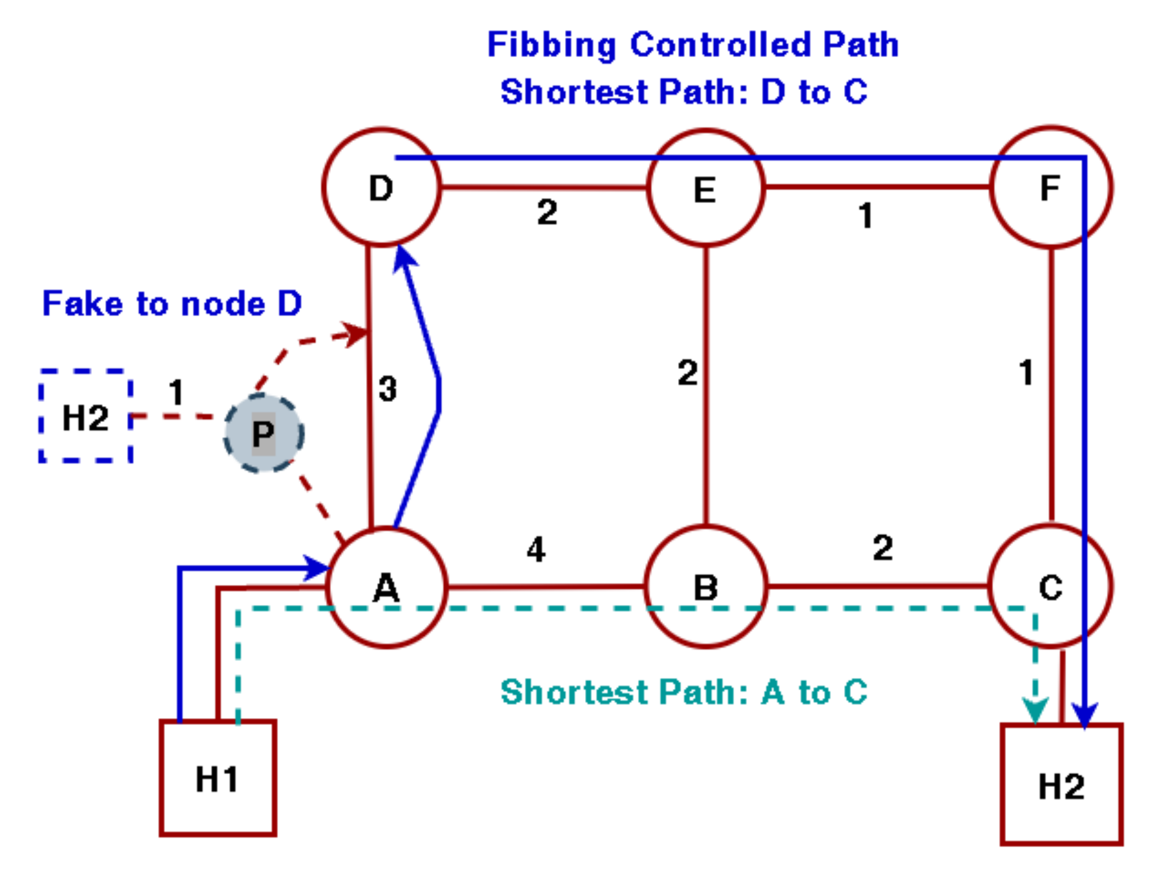
An example is shown in Figure 1. There are six routers (A, B, C, D, E, F) in the network. In the absence of the fake node F, the flow from host H1 to host H2 follows H1➔A➔B➔C➔H2 which is the shortest path between H1 and H2. After insertion of the fake node P, the path cost from node P to host H2 is 1. As a result, the fake node P becomes the next-hop node for A, and the new path becomes H1➔A➔D➔E➔F➔C➔H2.
In [9], we formulate the load-balanced routing problem as an ILP program. The output of the ILP program is used to deploy the fake nodes to provision one path for each OD pair in the Fibbing controlled network. COYOTE [10] takes advantage of ECMP further to enhance network control flexibility in a Fibbing network. As a result, an OD pair can be assigned more than one path to deliver its traffic. More importantly, not only the desired routing paths but also the ratios to allocate demand to the paths can be specified. In [11], the authors take traffic uncertainty into consideration in a Fibbing network. An algorithm is proposed to determine the oblivious routing paths. In [12], we use Fibbing to design energy-efficient IP networks. The links carrying no traffic are turned off to reduce power consumption by steering network traffic onto the most energy-efficient working topology.
Although Fibbing significantly enhances the flexibility of traffic engineering capability in IP networks, achieving fast failure recovery in a Fibbing network is not well addressed. Traditionally, an IP network running OSPF takes a long time to converge after a failure. The Loop-Free Alternative (LFA) [13] technology is the most typical approach to achieve fast failure recovery in an IP network to speed up failovers.
When a network failure happens, a router can reroute flows blocked by the failure device to its neighbor nodes if such rerouting does not generate any traffic loops. This is the key idea of loop-free alternate (LFA). For example, requirement (1) can reroute traffic when a single link failure happens. When (1) is fulfilled, X can send packets/data with destination address D to its neighbor node Y without generating loops. Besides (1), other requirements can be used to guarantee loop-free routing. For example, (2) can be used to ensure loop-free rerouting after a node failure or even multiple failures in an IP network.
Although (1) and (2) ensure loop-free rerouting, we found that LFA technology is not compatible with Fibbing [14]. If we apply LFA technology directly into the fibbing network, it is possible to generate traffic loops. In [14], we have developed a cycle-based monitoring approach to detect the failure in a Fibbing network. The failure detection time is proportional to the frequency of the delivery of the monitoring packets. The Fibbing controller can increase the frequency to achieve fast failure recovery, but it introduces more monitoring packets in the network. In addition, the detection time is also related to the number of nodes on the monitoring cycles. As the network becomes large, the Fibbing controller takes a longer time to detect a network failure.
In this work, we jointly take network load balancing and fast failure recovery into consideration. Our target is to provide working paths that can provide 100% survivability against any single node or link failure. We consider the property of LFA. When a failure is detected, the network nodes only need to follow typical LFA to reroute affected flows so the network can recover from a failure after a short time. We propose ILP (Integer Linear Programming) models for the problem. The output of the programs is used to determine the deployment of fake nodes so the desired load-balanced routing paths and preplanned backup paths can be realized.
The remaining parts of this paper are organized as follows: in Section 2, we present the requirements to guarantee loop-free rerouting. In Section 3, we present the ILP problem formulations for the problem. We have applied the proposed algorithm in multiple well-known benchmark networks and randomly generated networks. Section 4 demonstrates the numerical results. At the end of the paper, we provide concluding remarks in Section 5.
2. Requirements of Loop-Free Rerouting
Routers follow destination routing to forward the packet in IP networks. Although an IP packet carries source and destination addresses, routers only examine the destination address to obtain the next-hop node for packet forwarding. After the insertion of fake nodes, the paths generated by a Fibbing network must be loop-free. More specifically, the collection of the links used to forward packets to any destination node forms an acyclic graph in a Fibbing network. COYOTE cleverly takes ECMP rules to enhance routing flexibility in Fibbing networks. As a result, given an acyclic graph to a destination node and the flow splitting ratios, a set of fake nodes can be generated to realize the desired paths.
Although COYOTE provides an implementation for routing paths assignment, the working paths are not guaranteed to be survivable after a network failure. This section presents the requirements for a Fibbing network running LFA so the traffic carried by the working paths can be rerouted to bypass a failed node or a failed link.
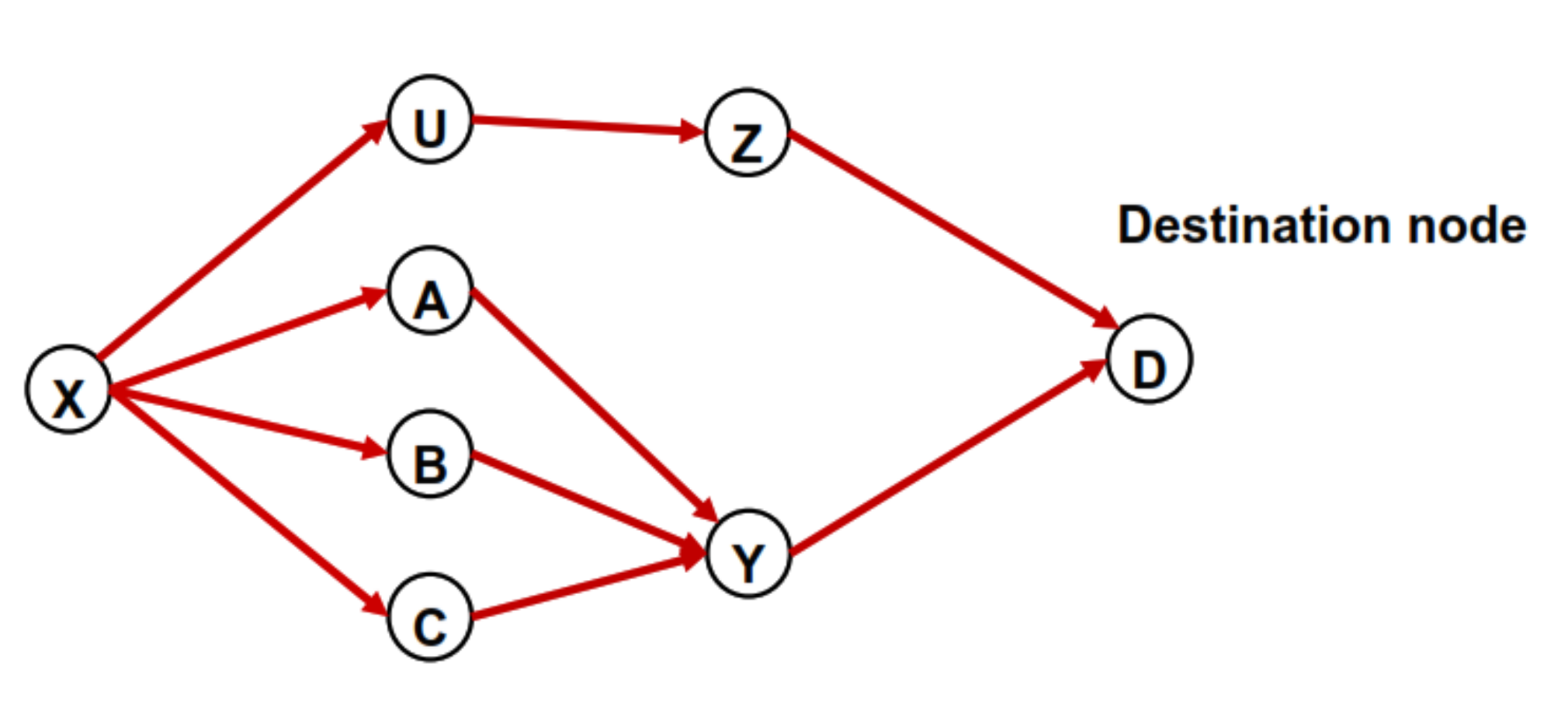
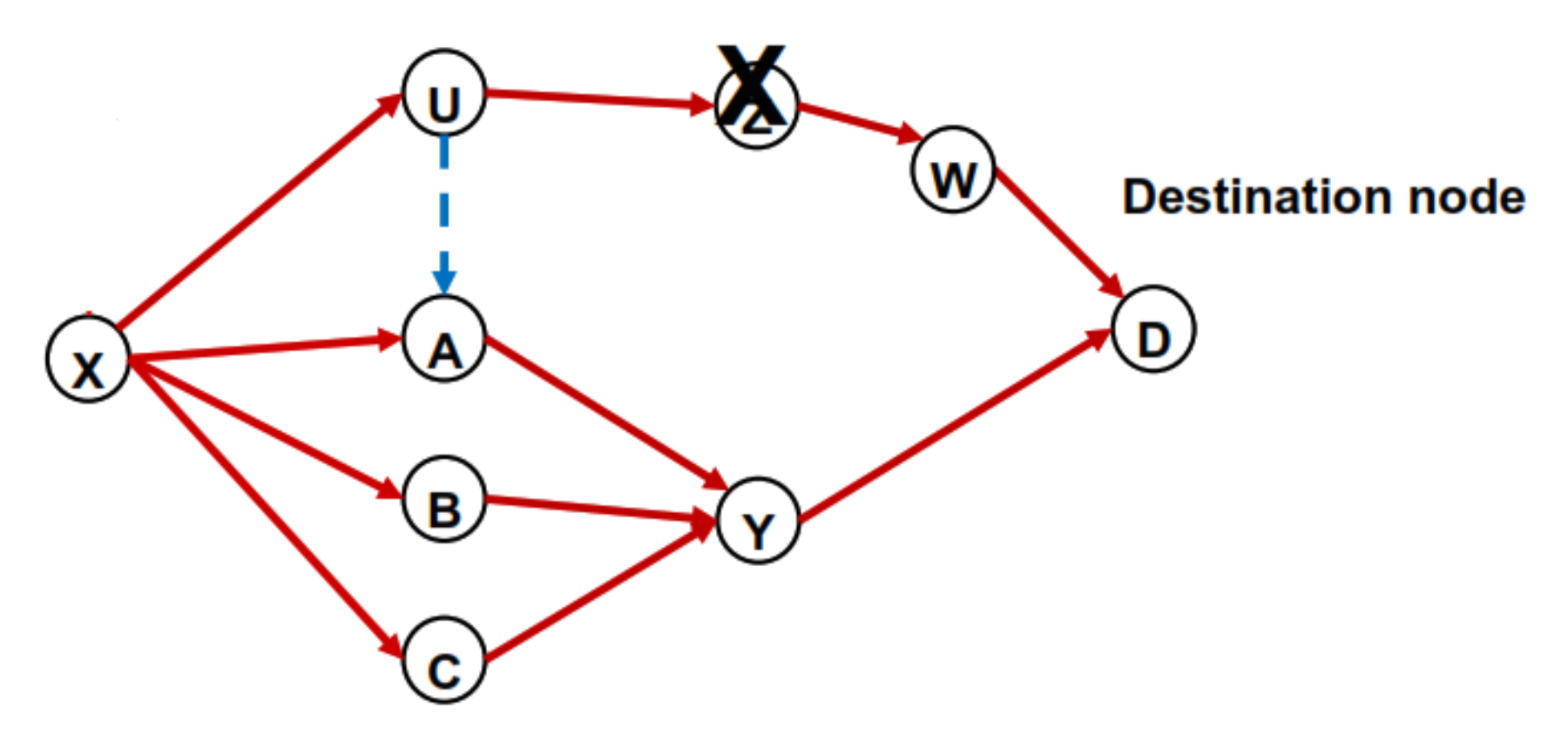
Because a single node and a single link failure are the most common failure events, we focus on handling these two types of failure. As we have mentioned, in a Fibbing network, the collection of the links used by the working paths toward a destination node must be an acyclic graph. We use the acyclic graph shown in Figure 2 as an example to illustrate the paths used for the destination node D. In this example, if node A is the starting node of a flow, this flow follows A➔Y➔D to deliver traffic to the destination node D. It is also possible that there are multiple paths between a source and a destination node pair. In this example, X uses four paths to deliver traffic to D.
2.1. Requirement to Reroute Traffic without Generating Traffic Loops
When a downstream node fails, the adjacent upstream node has to reroute the traffic to bypass the failed node or the failed link. The reroute traffic cannot form any loops. Three neighbor nodes can be used as a new next-hop node for an upstream node to reroute the interrupted traffic. The three kinds of neighbor nodes can be used for a single node failure case or a single link failure case. In the sequel, we call the whole network in the normal state if every node and link are actively working; otherwise, we call a network in a failure state. A flow follows its working path to its destination if the network is in its normal state. As soon as a node discovers a network failure, it follows LFA to reroute interrupted flows to another neighbor node to bypass the failure device.
R1 neighbor:
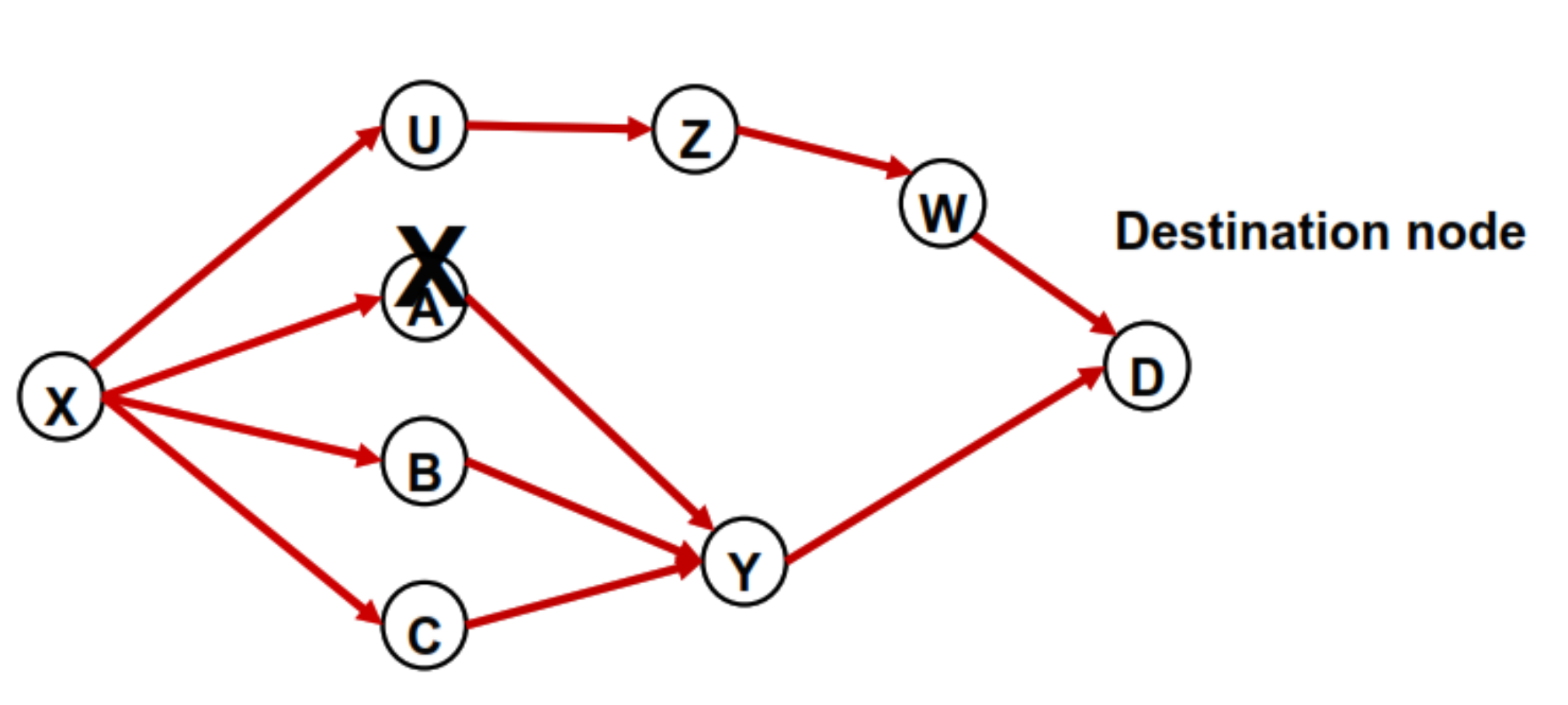
An upstream node N1 can reroute traffic to its neighbor node N2 if the link (N1, N2) is already in the acyclic graph. As shown in Figure 3, in the normal state, node X has four next hops for traffic toward destination D. When node A fails, X can use the other two next hop nodes U, B, and C to take over the traffic originally going through A. This method also works for a single link failure case. For example, if the failure link is (X, A), node X can reroute the interrupted traffic to U, B, or C without generating any loops. Because an R1 neighbor is a downstream node that has already been used to carry traffic toward destination D, we do not need to insert any additional fake nodes to enable the reroute. In the example, U, B, and C automatically meet the LFA requirement. As a result, when node A or link (X, A) fails, X can successfully reroute traffic through either U, B, or C for packets with destination D.
R2 neighbor:
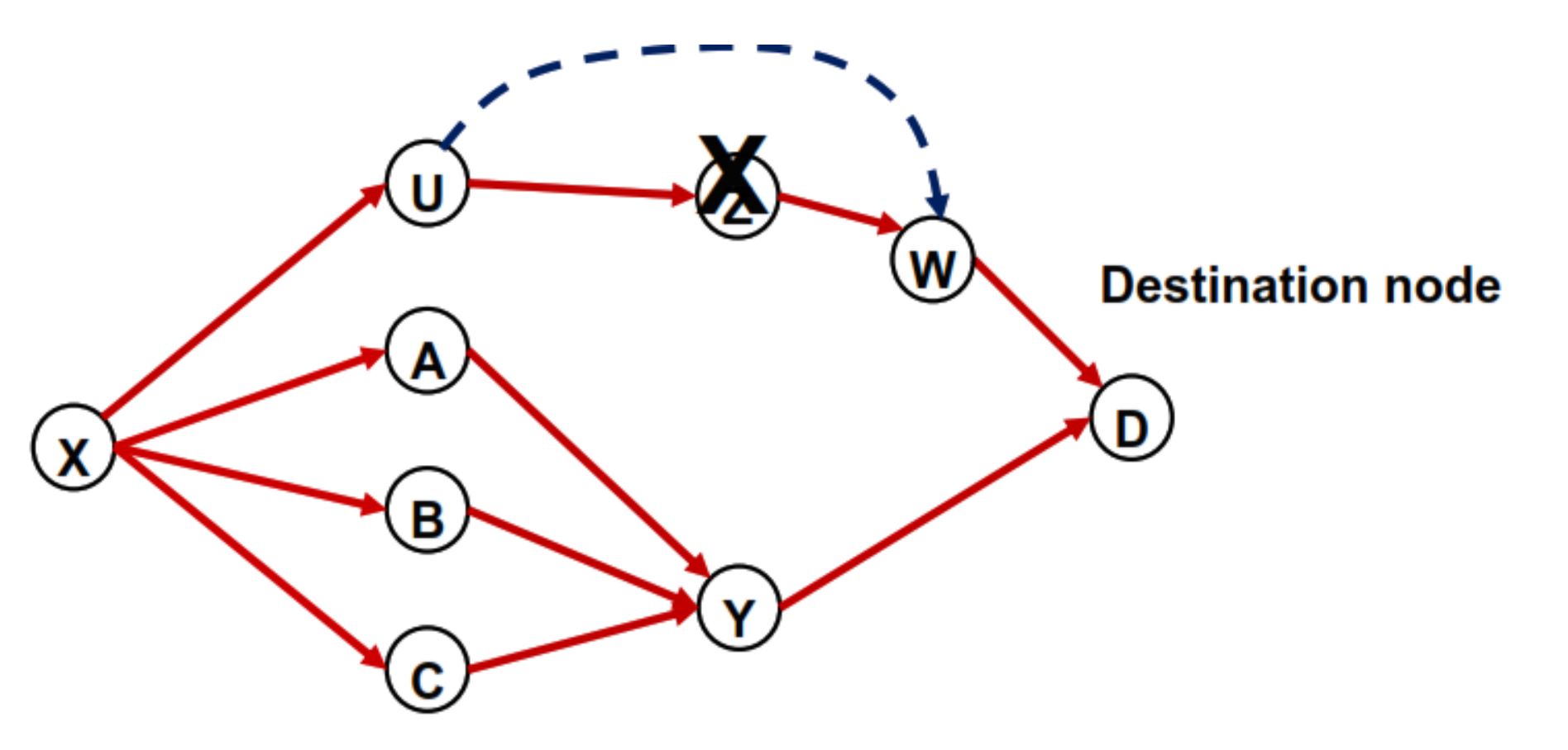
An upstream node N1 can reroute traffic to its neighbor node N2 if node N2 is a downstream node of node N1 in the acyclic graph. In Figure 4, node U has only one next-hop node (i.e., node Z). When node Z fails, node U does not have a neighbor node in the acyclic graph that meets the R1 neighbor requirement. However, if U has a link to a neighbor node downstream in the acyclic graph, U can redirect the flow with destination D to the downstream neighbor without generating loops. For example, if node W is a neighbor node of node U, node U can redirect the interrupted traffic to node W through the link (U, W). R2 neighbor can be used not only to protect a single node failure but also to protect single link failure. If the failed link is (U, Z), node U can reroute the interrupted traffic to W.
Please note that link (U, W) is not included in the acyclic graph with links used by the traffic in the normal case. This indicates that link (U, W) is not used to carry traffic for packets with destination D when the network is in the normal state.
Because an R2 neighbor is not used to carrying traffic towards destination D in the normal state, a fake node needs to be inserted in the network to enable an R2 neighbor to become a next-hop node when a failure happens. For example, suppose we want node W to become the next hop node after the failure of node Z or link (U, Z). In that case, we can introduce a new fake node with a cost higher than the shortest path cost seen by U. Hence, in the normal state, U sends the flow to Z but not W. As the failure happens, W becomes an eligible next hop based on the LFA rules.
R3 neighbor:
A node N1 can redirect flow to a neighbor N2 if N2 is neither a downstream node nor an upstream node of N1. In other words, the neighbor node belongs to another branch in the acyclic graph formed by the working paths. Figure 5 depicts the example. As node Z fails, node U can redirect the traffic to node A if the link (U, A) exists in the network. In this example, after receiving the redirected traffic, node A will send the traffic to its next-hop node, i.e., Y. Because A is not an upstream node of U, the rerouted traffic will not go back to U. It guarantees loop-free rerouting. The R3 neighbor requirement still holds for handling a single link failure. If the failure link is (U, Z), node U can forward the affected traffic to A for failure recovery. A fake node associated with link (U, A) needs to be inserted to realize the reroute. The cost introduced by the fake node need to be higher than the path cost seen by U. Consequently, U sends the traffic with destination D to node Z in the normal state. When Z or (U, Z) is failed, node A becomes the new next-hop node by the LFA rule.
For a node N1, if its neighbor node N2 is not an R1, R2, or R3 neighbor, N2 must be an upstream node in the acyclic graph generated by the working paths. Therefore, to guarantee 100% survivability, the assignment of the working paths needs to be carefully designed to ensure that every node in the acyclic graph must have at least one of the three types of neighbors. The requirement is used in our problem formulations shown in the next section, so any single node or link failure can be recovered in our networks.
2.2. OSPF Link Weight and Fake Node Assignment
Given the desired working paths and that every node in the acyclic graph generated by the working paths has at least one R1, R2, or R3 neighbor, we need to assign OSPF weight and fake node assignment to let the flows follow the desired routing paths in the normal state. In addition, we also need to deploy some fake nodes so the network can successfully recover from a failure.
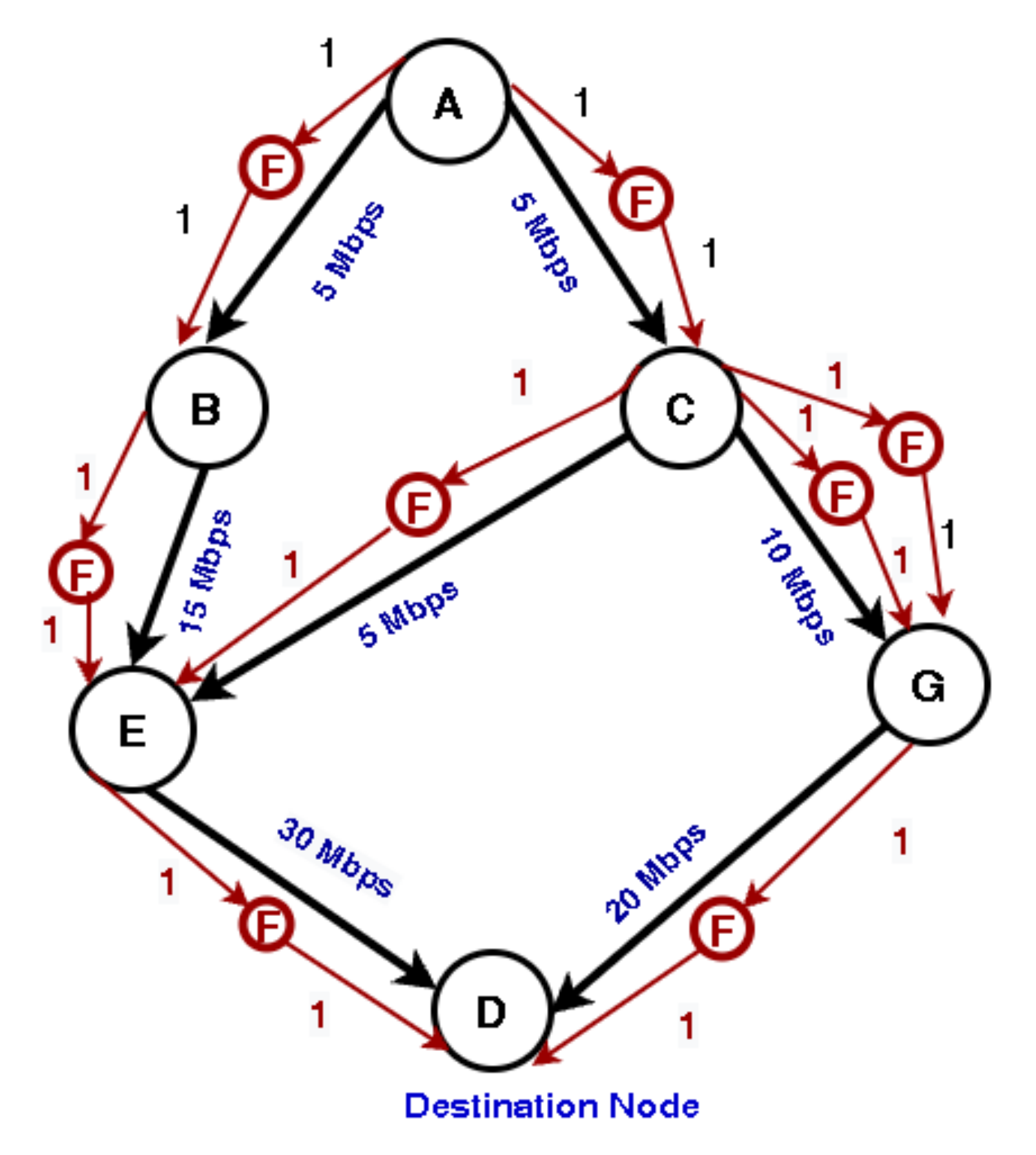
We apply the same technique introduced in COYOTE to deploy fake nodes to realize the routing for working paths. As shown in Figure 6, the acyclic graph represents the routing paths toward destination node D. Each node sends 5 Mbps to D. The demand volume carried by each link is indicated in the graph. The total demand from C to D is 15 Mbps (5 Mbps from A and 10 Mbps from C). If we want the two outgoing links (C, G) and (C, E) to carry 10 and 5 Mbps, respectively, the splitting ratios for link (C, G) and (C, E) are 2:1. Therefore, two fake nodes and one fake node are deployed associated with link (C, G) and (C, E), respectively. As a result, C follows the ECMP rule to split the traffic to (C, G) and (C, E) with the target ratio 2 and 1.
In our system, the OSPF weight for each link is assigned to be 10 and the weight for the fake link is one. To simplify this example, we do not include the backup path planning in this example. To deploy a R2 neighbor or a R3 neighbor, we need to introduce an additional fake node. For example, if there is a link (B, C) in the physical network, node C is a R3 neighbor of node B because they are in different branches. We can generate a fake node associated with link (B, C) with path cost 2. In the normal state, E is the only next hop node of B. As node E or link (B, E) fails, node B will take C to reroute the traffic with destination node D. Since the traffic reroute is triggered by LFA, the network can recover a failure within a very short time. We can apply the same technique to generate a fake node for the R3 neighbor. After inserting the fake nodes to enable R2 and R3 neighbors, the network is guaranteed to be 100% survivable against any single node or single link failure.
3. Optimization Models
This section presents the proposed ILP models for working and backup path planning in a Fibbing-controlled IP network. The objective function of these optimization models is to minimize the load on the most congested link when the network is in its normal state. We include network survivability constraints so every upstream node can have at least one neighbor node with either an R1, R2, or R3 neighbor. The output of the ILP programs is used to configure fake nodes in the network. To make comparisons, we first present the LBO formulation that only considers load balancing. Because the survivability constraints are not included in the formulation, the working paths obtained from the problem minimize the load on the most congested link. We use the results from LBO as a lower bound to justify the results when survivability constraints are included.
3.1. Load Balancing Only (LBO)
The problem formulation and notations are listed below.
Input Constants:
| set of routers in the network; | |
| L: | set of directional links in the network; |
| set of links leaving node n; | |
| set of links entering node n; | |
| the capacity of link l; | |
| demand volume from source node n to destination node d. |
Decision Variables:
| utilization on the most congested link; | |
| total traffic with destination d carried on link l. |
Problem (LBO):
| min u | ||
| Subject to: | ||
| (1) | ||
| (2) | ||
| (3) | ||
| (4) | ||
| (5) |
The Objective Function (OF) of this ILP is to minimize the link utilization on the most congested link. The first constraint (1) is the flow conservation law. Constraint (2) states that the total outgoing flow from the destination node must be zero, which means there is no flow leaving the destination node. Constraint (3) is the flow conservation law at the destination node d. Constraint (4) indicates that the sum of all the flows on each link must be less than the upper bound of the capacity.
3.2. Load Balancing and Node Failure Protection (LB&NFP)
The second formulation determines working and backup path assignments to protect against any single node failure. Given a destination node, the collection of links used in the routing paths must become an acyclic graph. This property is true for the network operating in a normal state and true under any single node failure state. To maintain flow routing in an acyclic graph toward every destination node, we introduce the concept of node potential to facilitate the problem formulation. A packet can only be sent from a node with high potential to a node with low potential. This rule is applied for the packets forwarding in the normal state and the backup state. Because a flow can only be delivered from a high potential node to a low potential node, the routing path is guaranteed to be loop-free whether the network is in the normal or a failure state.
Because we consider every node failure, the total number of failure states is the same as the number of nodes in the network. Each failure state is mapped to a single node in the network. The meaning of N, L, , , , and are the same as those used in the LBO formulation. The additional notations are listed below.
Input Constants:
| the head node of link l; | |
| the tail node of link l; | |
| a big number; | |
| set of nodes that are neighbors of node s. |
Decision Variables:
| utilization on the most congested link; | |
| total traffic with destination d carried on link l; | |
| =1, if link l is used to carry traffic with destination d in the normal state; =0, otherwise; | |
| =1, if link l can be used to reroute packets with destination d in state s =0, otherwise; | |
| the potential difference between node n to node d when network is in state s. |
Problem (LB&NFP):
| min u | ||
| Subject to: | ||
| (6) | ||
| (7) | ||
| (8) | ||
| (9) | ||
| (10) | ||
| (11) | ||
| (12) | ||
| (13) | ||
| (14) | ||
| (15) | ||
| (16) | ||
| (17) | ||
| (18) |
For a directional link l = (a, b), traffic using the link must visit node a before node b. Hence, we call node a the upstream node, and node b is the downstream node of this link l. The first four constraints have appeared in Problem LBO. Constraint (10) is used to determine which link can deliver traffic in the normal state. If is non-zero, which means link l is used to carry traffic with destination d in the normal state, it results in becoming 1. Constraints (11), (12), and (13) are constraints to determine node potential. We have mentioned that if a feasible set of node potentials can be assigned to each node in every single node failure state, we can guarantee loop-free routing in the network. For destination node d, Constraint (11) requires that if link l is used to carry traffic with destination d in the normal state, the potential of the upstream node of link l must be higher than the potential of the downstream node of link l. Because any non-zero enforces become 1, if link l is used to carry traffic with destination d in the normal state, the potential of the upstream node of link l must be higher than the potential of the downstream node of link l. More specifically, no matter the network is operating in which state s, any path (n1, n2, …, d) that is used to carry non-zero traffic with destination node d in the normal state, the order of node potential is >…>.
Constraint (11) enforces the order of potential nodes within a single path (i.e., a traffic branch). However, it does not restrict the relationship between two nodes that belong to different branches. To enable taking an R3 neighbor to reroute traffic, we include Constraint (12) in the formulation. When a node failure happens, an upstream node with high potential can reroute, interrupting traffic to a neighbor with low potential if it is a node in a different branch. Because we only allow traffic to be delivered from a high potential node to a low potential node, loop free is guaranteed in the network whether it is in the normal or failure state.
Constraint (14) guarantees 100% survivability against any single node failure. It requires that every node has at least one neighbor node to reroute traffic while the network is in a failure state. On the left-hand side of the constraint, when node s fails, every node n that is a neighbor of s must still be able to send its traffic to destination d. After excluding the link (n, s), if node n has a link with or means node n has a higher potential than the head node of link l, and node n can take link l to deliver traffic with destination d without generating any loops.
Based on the output of LB&NLP, we can determine the deployment of the fake nodes. The acyclic graph for the working paths can be obtained by collecting the links with a non-zero value of x. The backup path planning can be derived from y and z. Suppose node n uses multiple outgoing links to carry traffic with destination d in the normal state. In that case, we do not need to deploy additional fake nodes for n to reroute traffic against any of its downstream node failures. This is the case of node X shown in Figure 3. Node X always has an R1 neighbor to recover the failure. Suppose node n has only one single next-hop node j for traffic delivery with destination d. We have to deploy a fake node to reroute the traffic when j fails. The neighbor for the reroute is either an R2 or an R3 neighbor. According to Constraint (14), there must be at least one outgoing link l of node n with or . We can select any link l with or to be used for node n to reroute traffic with destination d.
3.3. Load Balancing and Link Failure Protection (LB&LFP)
Problem LB&LFP is used to determine load-balanced routing and backup paths planning to protect any single link failure. The decision variables have the same meaning as those used in Problem LB&NFP. The additional input constants used in the problem are set S and In most communication networks, if two nodes, x, and y are neighbor nodes to each other, there are two directional links, (x,y) and (y,x), between them. When a link failure event disconnects the two neighbor nodes x and y, we assume both directional links (x,y) and (y,x) cannot transmit packets anymore. Therefore, for every link failure event, two-directional links are failed in the formulation. Our model can be modified for the network if each failure event only results in a single directional link failure. Since the techniques used in the formulation are the same as those used in Problem LB&NFP, we directly include the formulation below and skip detailed expression for each constraint.
Input Constants:
| S: | failure set; |
| the two-directional links that become failed when event s happens. |
Problem (LB&LFP):
| min u | ||
| Subject to: | ||
| (19) | ||
| (20) | ||
| (21) | ||
| (22) | ||
| (23) | ||
| (24) | ||
| (25) | ||
| (26) | ||
| (27) | ||
| (28) | ||
| : | (29) | |
| (30) | ||
| (31) |
4. Numerical Results and Discussions
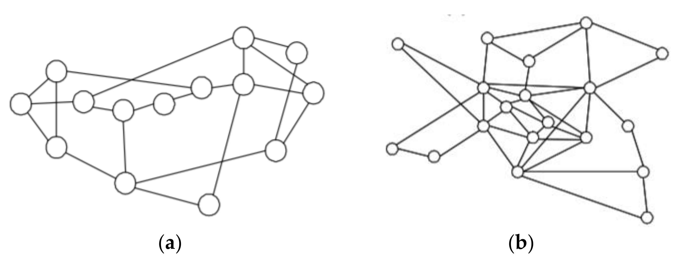
We use CPLEX to implement the three programs (LBO, LB&NFP, LB&LFP). We evaluate our ILP models on two sets of topologies. The first topologies come from four well-known networks shown in Figure 7. The link capacity for every link is 100 units. Each node pair in the network has a one-unit demand. The topologies in the second set are randomly generated. The connectivity of each topology is at least 2-Vertex and 3-Edges (2V3E). Each node pair in the network is assigned a random demand with demand volume obtained from the Bimodal Traffic Matrices (TMs) [15]. We combine the two Gaussians. The first is () and the second is (), to generate Bimodal traffic demands. The first Gaussian generates small traffic demand, and the second Gaussian generates large (big) traffic demand. A biased coin is flipped for every OD pair, for which the chances (probability) of head and tail are 0.8 and 0.2, respectively. The random number is produced using the first Gaussian () if a flipped coin shows heads; otherwise, second Gaussian TMs are used. Thus, we have 80% small demand and 20% large (big) demand. We set the value of the error margin as two.
4.1. Utilization on the Most Congested Link
The results obtained from Problem LBO is a lower bound to Problem LB&NFP and Problem LB&LFP; we use the normalized index to evaluate the utilization on the most congested link. For node protection cases, the normalized index is the objective function value of Problem LB&NFP divided by the objective function value of LBO. For the link protection case, the normalized index is the objective function value of Problem LB&LFP divided by the objective function value of LBO.
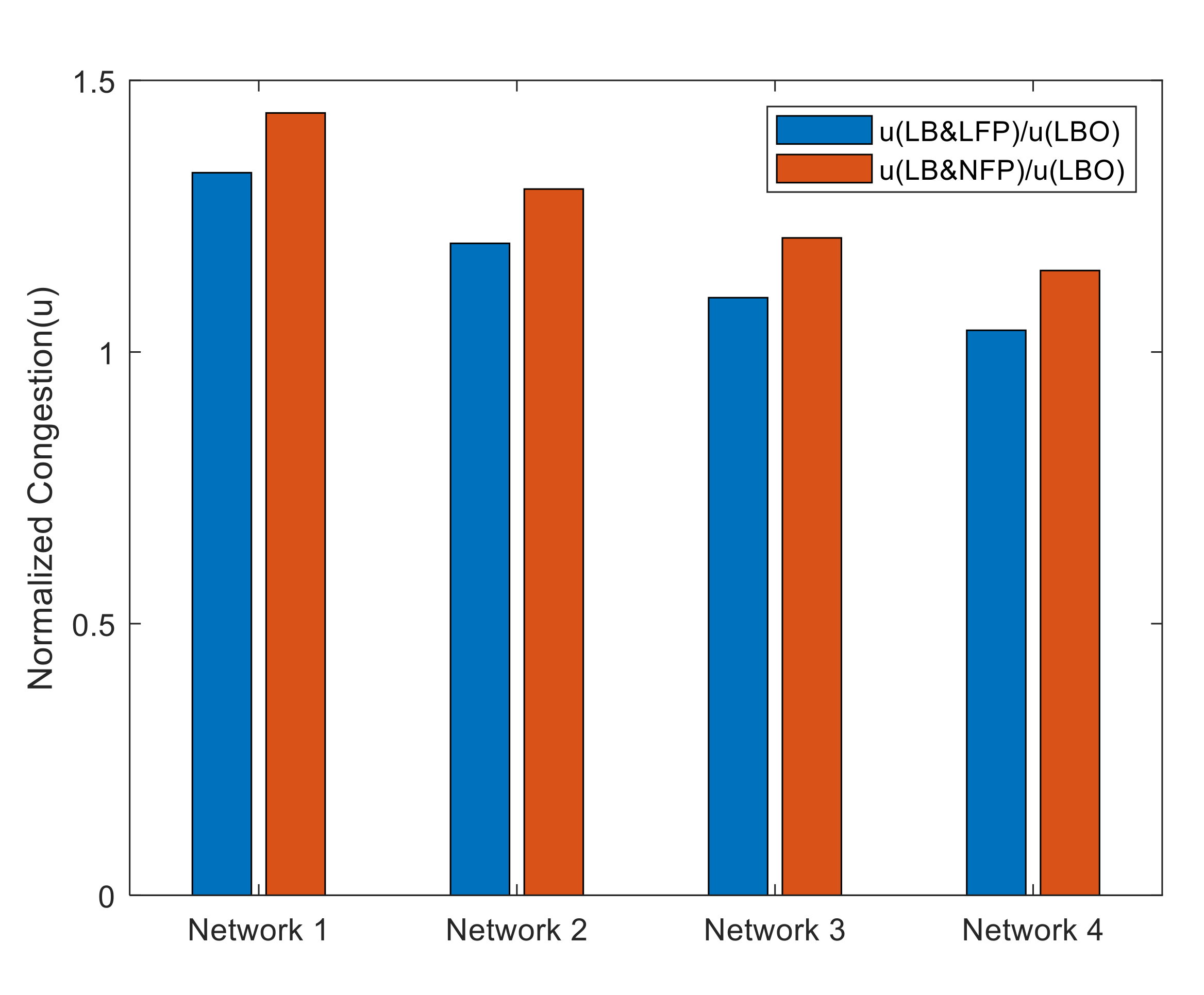
Table 1 shows the normalized values of problem LB&LFP and LB&NFP. In case of LB&LFP, the network 1 normalized congestion value is 1.33, and the network 4 value is 1.02. As the size of the network increases, the normalized congestion value starts to decrease and makes the network recovery faster for any single node and link failure. In case of LB&NFP, all networks depicts similar trends as in LB&LFP; the network 1 normalized index is 1.44 and network 4 is 1.15. Therefore, the larger the network, the smaller the congestion. When a node failure event happens, the network consumes more bandwidth as compared to a link failure event. As shown in Figure 8, normalized congestion values of LB&NFP are higher than LB&LFP, because in a node failure event, multiple links are removed from the network. Hence, the congestion values of LB&NFP are upper bound to LB&LFP.
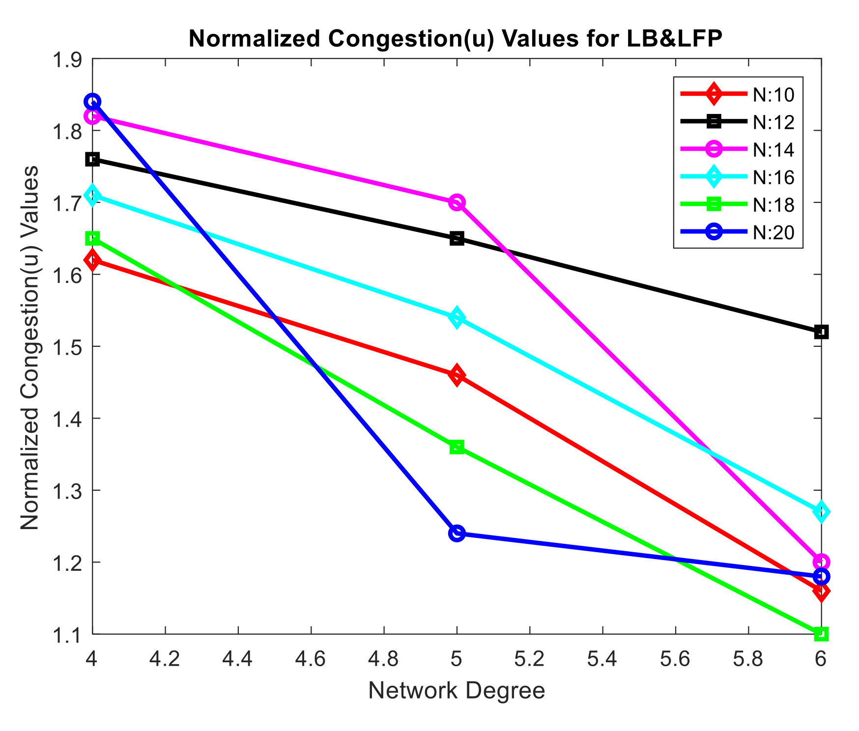
We further test our optimization models on randomly generated networks. Table 2 shows the normalized congestion values in the instance of LB&LFP. A normalized congestion value of 1.62 exists in the network with node 10 and degree 4, and a value of 1.16 exists in the network with node 10 and degree 6. Congestion numbers decrease as the degree in the network grows. The normalized congestion values of randomly generated networks for LB&LFP are shown in Figure 9. The x-axis of the graph displays the network’s degree, while the y-axis shows the normalized congestion values. The red curve in the graph represents a network with ten nodes. The normalized index for the Node 10 network is 1.62 when the degree is four, 1.46 when the degree is five, and 1.16 when the degree is six. As shown in the graph, the normalized index is 1.62 when the degree is four, 1.46 when the degree is five, and 1.16 when the degree is six. As a result, as the network’s degree grows, the normalized congestion value drops. From node 12 through node 20, the other networks follow the same pattern.
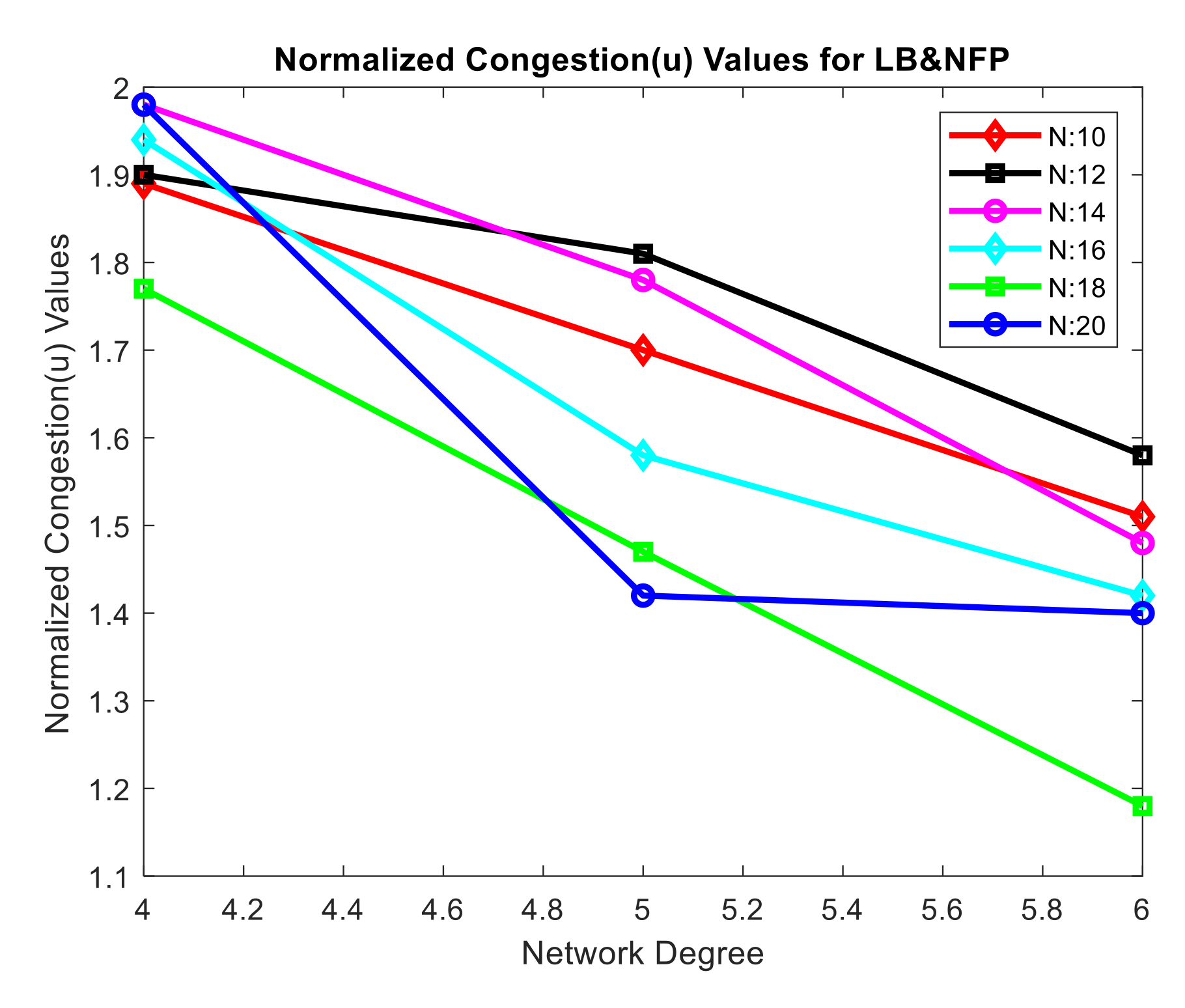
The normalized congestion values for LB&NFP are shown in Table 3. It has the same pattern as LB&LFP. A normalized congestion value of 1.94 exists in the network with node 16 and degree 4. The normalized index is 1.58 when the degree is five, and it is 1.42 when the degree is six. The size of the network grows as the degree of the network grows, and the network’s congestion decreases. As a result, the recovery of a network after a failure is sped up.
Figure 10 shows the normalized congestion (u) values of randomly constructed LB&NFP networks. When the degree of the node 18 network is four, the normalized value is 1.77, whereas when the degree is six, the value is 1.18. It indicates that when the network’s degree grows, the normalized congestion (u) values drop, following the same trend as LB&LFP.
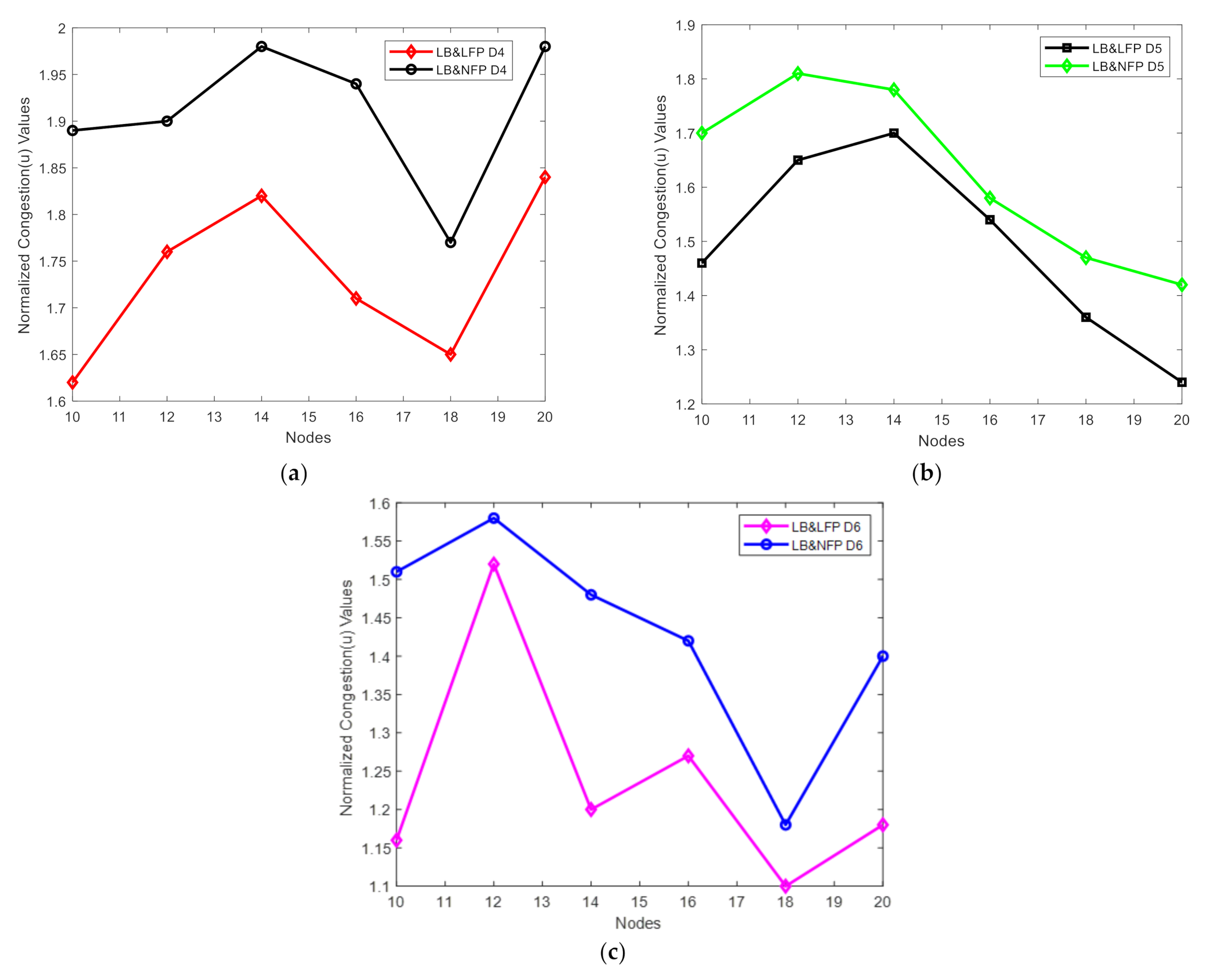
Figure 11 shows the comparisons of normalized congestion values for degree 4, 5, and 6 networks for LB&LFP and LB&NFP. We compare LB&LFP and LB&NFP results based on their normalized congestion values. We find that the normalized congestion value of LB&LFP is lower bound to LB&NFP because the link failure event consumes less bandwidth than node failure. A node failure means multiple links are removed from the network, so that is why its normalized congestion value is greater compared to the link failure.
4.2. Network Survivability
Network survivability refers to a network’s capacity to continue providing services in the event of a failure [16]. Our optimization models (LB&LFP and LB&NFP) guarantee network survival in the event of node or link failure.
4.2.1. Node Protection
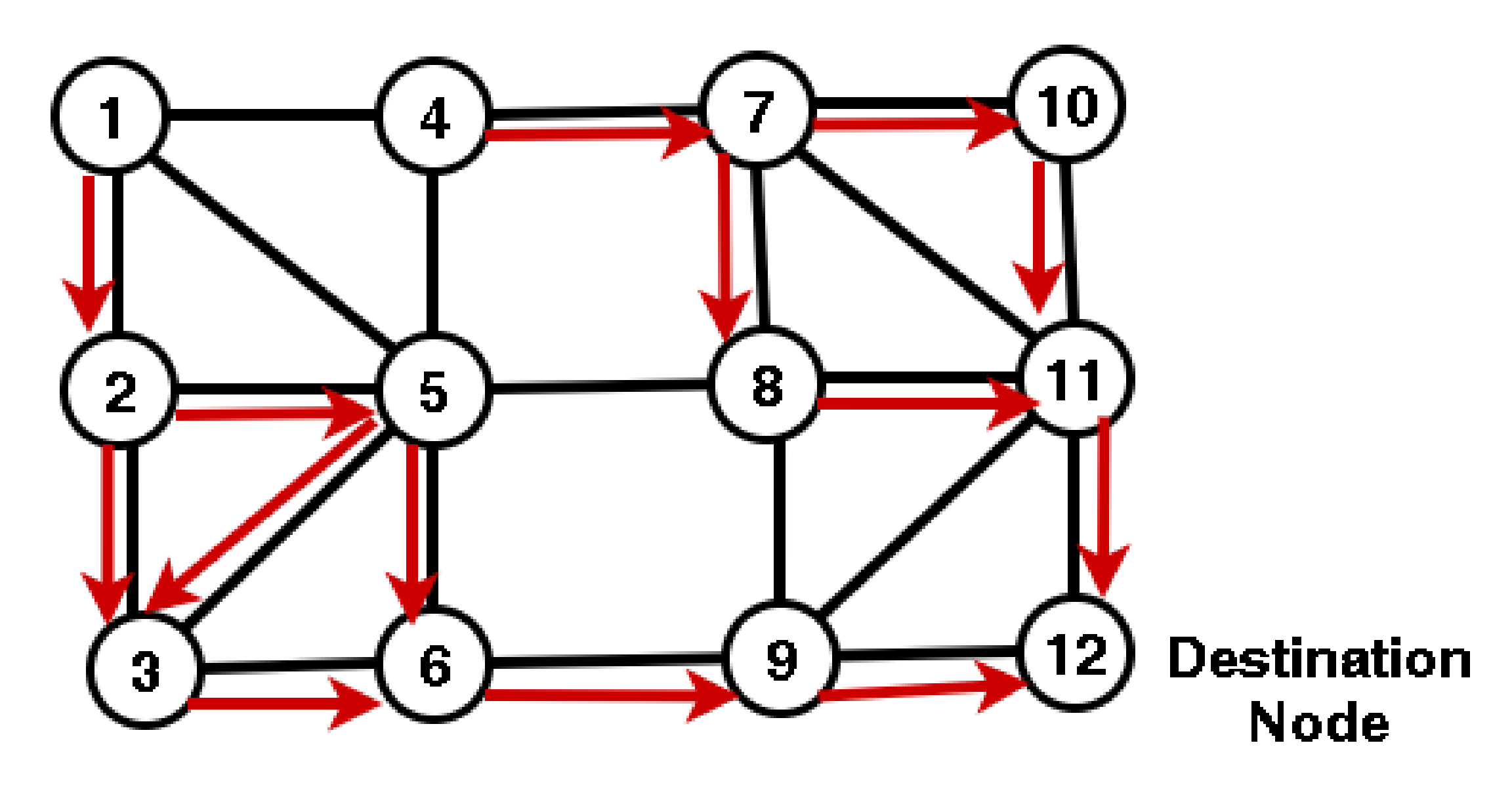
Figure 12 depicts a network with twelve nodes. The source node is node 1, while the destination node is node 12. The working traffic towards the destination node is shown by the red links. Our optimization model “LBO” provides us this solution (red links).
We solve the LBO model for node protection and determine whether or not the flow is survivable. We get the routing for each OD pair after solving this model. For example, when node 6 fails, node 3 has no LFA. It means node 3 is not survivable. When node 9 fails, node 6 has no LFA. When node 11 fails, node 10 has no LFA. We analyze this for each OD pair. When node 8 fails, traffic to destination node 12 can be recovered.
We define survivability as:
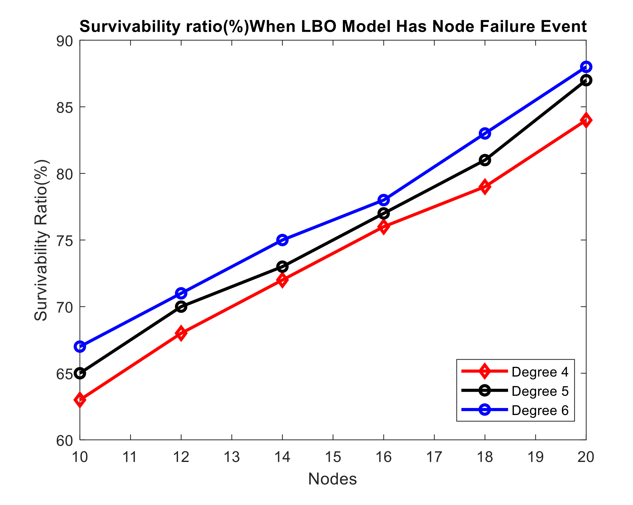
We find the survivability ratios when the LBO problem encounters a node failure. When a node fails in the network, as illustrated in Table 4, the network is not 100% survivable. The network’s survivability ratio increases as the network’s size grows. The trends in survival ratio are shown in Figure 13. The survivability ratio of a network grows as the degree and number of nodes increase. As a result, when a node fails, the LBO model is not 100% survivable. As a result, our LB&NFP problem guarantees network survival. The LB&NFP problem’s 14th constraint provides 100 percent survivability.
4.2.2. Link Protection
If we look at Figure 12 for a link failure event, we can see that when link (3,6) fails for destination node 12, node 3 has no LFA, node 6 has no LFA if link (6,9) fails, and so on. The network will not be 100% survivable in case of link failure. We define the survivability for link failure as:
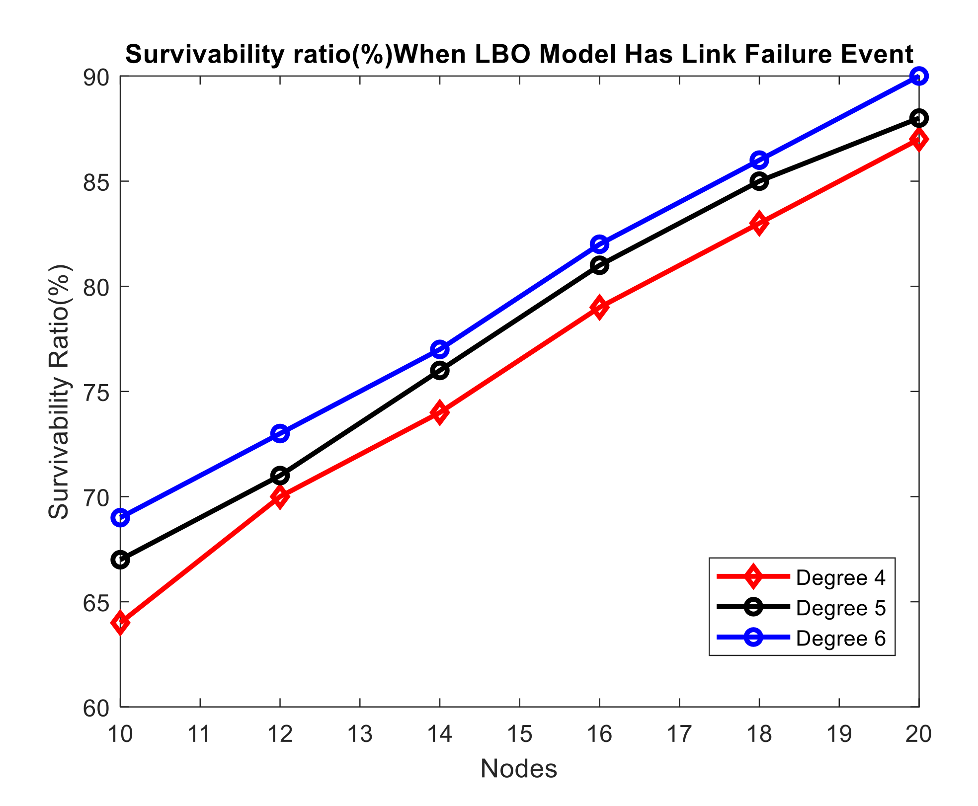
When the LBO problem experiences a link failure, we calculate the survivability ratios. When there is a link failure event in the network, as illustrated in Table 5, it is not 100 percent survivable. Figure 14 demonstrates that when the size of the network grows (in terms of the number of nodes and the degree of the network), the survivability ratio grows as well. These, however, are not 100% survivable. When a node fails, the survivability ratios are lower than when a link fails. Our LB&LFP optimization model ensures network viability at all times. In the LB&LFP problem, the 27th constraint assures 100 percent survivability in the presence of a single link failure.
5. Conclusions
A network must be able to efficiently manage the traffic routing to improve utilization and to prevent congestion. IP networks are reliable and robust due to distributed link-state routing protocols, even though, relatively, routing is not flexible in IP networks. Fibbing is a new approach that achieves flexibility and robustness with centralized control over distributed routing. Even though a Fibbing approach offers flexible routing in IP networks, strategies for attaining fast recovery from failures have not been thoroughly examined. To speed up failovers, the IP fast reroute, Loop-Free Alternative (LFA) technology, is proposed by IETF. We found that LFA technology with Fibbing is not compatible. Traffic loops will result if LFA technology is used directly with the Fibbing network. We offer workable pathways that guarantee 100 percent survivability in the event of a single node or single link failure. We offer ILP (Integer Linear Programming) models. The output of the programs is used to calculate the placement of fake nodes in order to achieve the appropriate load-balanced routing paths and backup paths. We use a CPLEX optimization solver for LBO, LB&LFP, and LB&NFP models. The objective function of our optimization models is to minimize the utilization of the most congested link. We put our models to the test under both fixed and random traffic demands. Our optimization models give optimal solution for these three models. The results show that the system identifies single node and link failures and assigns a routing path for load balancing and fast failure recovery by decreasing link utilization on the most congested link and ensuring 100% network survivability.
Author Contributions
Conceptualization, S.S.W.L.; software, M.I. and T.A.; validation, T.A.; formal analysis, T.A.; writing, T.A. and M.I.; supervision, S.S.W.L. and J.-Y.P.; project administration, S.S.W.L. and J.-Y.P. All authors have read and agreed to the published version of the manuscript.
Funding
This research was funded by the Ministry of Science and Technology of Taiwan under Grant MOST 108-2221-E-194-021-MY3.
Conflicts of Interest
The authors declare no conflict of interest.
References
- Pioro, M.; Medhi, D. Routing, Flow, and Capacity Design in Communication and Computer Networks; Elsevier, Morgan Kaufmann Publishers: San Francisco, CA, USA, 2004. [Google Scholar]
- Fortz, B.; Rexford, J.; Thorup, M. Traffic Engineering with Traditional IP Routing Protocols. IEEE Commun. Mag. 2002, 40, 118–124. [Google Scholar] [CrossRef] [Green Version]
- Wang, N.; Ho, K.; Pavlou, G.; Howarth, M. An Overview of Routing Optimization for Internet Traffic Engineering. IEEE Commun. Surv. Tutor. 2008, 10, 36–56. [Google Scholar] [CrossRef] [Green Version]
- Curtis, A.R.; Mogul, J.C.; Tourrilhes, J.; Yalagandula, P.; Sharma, P.; Banerjee, S. DevoFlow: Scaling Flow Management for High-performance Networks. In Proceedings of the ACM SIGCOM 2011 Conference, Toronto, ON, Canada, 15–19 August 2011; pp. 254–265. [Google Scholar]
- Ericsson, M.; Resende, M.; Pardalos, P. A genetic algorithm for the weight setting problem in OSPF routing. J. Comb. Optim. 2002, 6, 299–333. [Google Scholar] [CrossRef]
- Vissicchio, S.; Vanbever, L.; Rexford, J. Sweet little lies: Fake topologies for flexible routing. In Proceedings of the 13th ACM Workshop on Hot Topics in Networks, HotNets-XIII, Los Angeles, CA, USA, 27–28 October 2014; pp. 1–7. [Google Scholar]
- Vissicchio, S.; Tilmans, O.; Vanbever, L.; Rexford, J. Central control over distributed routing. In Proceedings of the 2015 ACM Conference on Special Interest Group on Data Communication, London, UK, 17–21 August 2015; pp. 43–56. [Google Scholar]
- Moy, J. OSPF Version 2; RFC 2328; RFC Editor: Marina del Rey, CA, USA, 1998. [Google Scholar] [CrossRef]
- Zanjani, S.B.; Li, K.; Lee, S.S.W.; Chu, Y. Path Provisioning for Fibbing Controlled Load Balanced IP Networks. In Proceedings of the 2018 IEEE Tenth International Conference on Ubiquitous and Future Networks (ICUFN), Prague, Czech Republic, 3–6 July 2018; pp. 154–158. [Google Scholar] [CrossRef]
- Chiesa, M.; Rétvári, G.; Schapira, M. Lying your way to better traffic engineering. In Proceedings of the 12th ACM International Conference on Emerging Networking EXperiments and Technologies, Irvine, CA, USA, 12–15 December 2016; pp. 391–398. [Google Scholar]
- Chiesa, M.; Rétvári, G.; Schapira, M. Oblivious Routing in IP Networks. IEEE/ACM Trans. Netw. 2018, 26, 1292–1305. [Google Scholar] [CrossRef]
- Lee, S.S.W.; Li, K.; Zanjani, S.B. Routing and Working Topology Assignment for Energy Efficient Fibbing-Controlled IP Networks. In Proceedings of the IEEE 2019 International Conference on IEEE Green Computing, Atlanta, GA, USA, 14–17 July 2019. [Google Scholar]
- Atlas, A.; Zinin, A. Basic Specification for IP Fast Reroute: Loop-Free Alternates. Request for Comments: 5286. Internet Engineering Task Force (IETF). 2008. Available online: https://tools.ietf.org/html/rfc5286 (accessed on 10 January 2021).
- Lee, S.S.W.; Chan, K.-Y.; Wong, T.-S.; Xiao, B.-X. A Fast Failure Recovery Scheme for Fibbing Networks. IEEE Open J. Commun. Soc. 2020, 1, 1196–1212. [Google Scholar] [CrossRef]
- Medina, A.; Taft, N.; Salamatian, K.; Bhattacharyya, S.; Diot, C. Traffic matrix estimation: Existing techniques and new directions. ACM SIGCOMM Comput. Commun. Rev. 2002, 32, 161–174. [Google Scholar] [CrossRef]
- Kuipers, F.A. An overview of algorithms for network survivability. Int. Sch. Res. Not. 2012. [Google Scholar] [CrossRef] [Green Version]
Figure 1.
Traffic flow in a Fibbing network.

Figure 2.
Acyclic graph generated by the working paths.

Figure 3.
Upstream node has multiple next hop nodes.

Figure 4.
Upstream node has a downstream neighbor node.

Figure 5.
Reroute through a neighbor node in another branch.

Figure 6.
OSPF weight and fake nodes assignment to realize the desired routing paths with given bifurcating ratios for traffic towards destination D in the normal state.
Figure 6.
OSPF weight and fake nodes assignment to realize the desired routing paths with given bifurcating ratios for traffic towards destination D in the normal state.

Figure 7.
Well-known benchmark networks [12]. (a) NSF network; (b) EON network; (c) COST239 Network; (d) USA network.
Figure 7.
Well-known benchmark networks [12]. (a) NSF network; (b) EON network; (c) COST239 Network; (d) USA network.


Figure 8.
Normalized congestion values for well-known networks.

Figure 9.
Randomly generated networks normalized congestion values for LB&LFP.

Figure 10.
Randomly generated networks normalized congestion values for LB&NFP.

Figure 11.
Comparisons of normalized congestion values for degree 4, 5, and 6 networks for LB&LFP and LB&NFP. (a) Degree 4; (b) degree 5; (c) degree 6.
Figure 11.
Comparisons of normalized congestion values for degree 4, 5, and 6 networks for LB&LFP and LB&NFP. (a) Degree 4; (b) degree 5; (c) degree 6.

Figure 12.
Network survivability.

Figure 13.
Survivability ratio (%) when LBO model has node failure event.

Figure 14.
Survivability ratio (%) when LBO model has a link failure Event.


Table 1.
Normalized congestion values for the four well-known benchmark networks.
| Benchmark Networks | u(LB&LFP)/u(LBO) | u(LB&NFP)/u(LBO) |
|---|---|---|
| Network 1 (NSF Network) | 1.33 | 1.44 |
| Network 2 (EON Network) | 1.20 | 1.30 |
| Network 3 (Cost239 Network) | 1.10 | 1.21 |
| Network 4 (USA Network) | 1.04 | 1.15 |
Table 2.
Randomly generated networks normalized congestion values for LB&LFP.
| Degree | N:10 | N:12 | N:14 | N:16 | N:18 | N:20 |
| 4 | 1.62 | 1.76 | 1.82 | 1.71 | 1.65 | 1.84 |
| 5 | 1.46 | 1.65 | 1.70 | 1.54 | 1.36 | 1.24 |
| 6 | 1.16 | 1.52 | 1.20 | 1.27 | 1.10 | 1.18 |
Table 3.
Randomly generated networks normalized congestion values for LB&NFP.
| Degree | N:10 | N:12 | N:14 | N:16 | N:18 | N:20 |
| 4 | 1.89 | 1.90 | 1.98 | 1.94 | 1.77 | 1.98 |
| 5 | 1.70 | 1.81 | 1.78 | 1.58 | 1.47 | 1.42 |
| 6 | 1.51 | 1.58 | 1.48 | 1.42 | 1.18 | 1.40 |
Table 4.
Survivability ratio (%) when LBO model has node failure event.
| Degree | N:10 | N:12 | N:14 | N:16 | N:18 | N:20 |
| 4 | 63 | 68 | 72 | 76 | 79 | 84 |
| 5 | 65 | 70 | 73 | 77 | 81 | 87 |
| 6 | 67 | 71 | 75 | 78 | 83 | 88 |
Table 5.
Survivability ratio (%) when LBO model has link failure event.
| Degree | N:10 | N:12 | N:14 | N:16 | N:18 | N:20 |
| 4 | 64 | 70 | 74 | 79 | 83 | 87 |
| 5 | 67 | 71 | 76 | 81 | 85 | 88 |
| 6 | 69 | 73 | 77 | 82 | 86 | 90 |
Publisher’s Note: MDPI stays neutral with regard to jurisdictional claims in published maps and institutional affiliations. |
© 2021 by the authors. Licensee MDPI, Basel, Switzerland. This article is an open access article distributed under the terms and conditions of the Creative Commons Attribution (CC BY) license (https://creativecommons.org/licenses/by/4.0/).
Share and Cite
MDPI and ACS Style
Ashraf, T.; Lee, S.S.W.; Iqbal, M.; Pan, J.-Y. Routing Path Assignment for Joint Load Balancing and Fast Failure Recovery in IP Network. Appl. Sci. 2021, 11, 10504. https://0-doi-org.brum.beds.ac.uk/10.3390/app112110504
AMA Style
Ashraf T, Lee SSW, Iqbal M, Pan J-Y. Routing Path Assignment for Joint Load Balancing and Fast Failure Recovery in IP Network. Applied Sciences. 2021; 11(21):10504. https://0-doi-org.brum.beds.ac.uk/10.3390/app112110504
Chicago/Turabian StyleAshraf, Tabinda, Steven S. W. Lee, Muhammad Iqbal, and Jen-Yi Pan. 2021. "Routing Path Assignment for Joint Load Balancing and Fast Failure Recovery in IP Network" Applied Sciences 11, no. 21: 10504. https://0-doi-org.brum.beds.ac.uk/10.3390/app112110504
Note that from the first issue of 2016, this journal uses article numbers instead of page numbers. See further details here.