
A Practical and Adaptive Approach to Predicting Indoor CO2
by
 , ,
, ,
Giacomo Segala
1,2,3,* ,
,
Roberto Doriguzzi-Corin
2,
Claudio Peroni
1,
Tommaso Gazzini
1 and
Domenico Siracusa
2 1
Energenius srl, 38068 Rovereto, Italy
2
Fondazione Bruno Kessler (FBK), 38123 Trento, Italy
3
Department of Information Engineering and Computer Science (DISI), University of Trento, 38123 Trento, Italy
*
Author to whom correspondence should be addressed.
Appl. Sci. 2021, 11(22), 10771; https://0-doi-org.brum.beds.ac.uk/10.3390/app112210771
Submission received: 13 September 2021
/
Revised: 5 November 2021
/
Accepted: 10 November 2021
/
Published: 15 November 2021
(This article belongs to the Special Issue New Insights into Ventilation, Comfort and Air Pollution)
Abstract
:COVID-19 has underlined the importance of monitoring indoor air quality (IAQ) to guarantee safe conditions in enclosed environments. Due to its strict correlation with human presence, carbon dioxide (CO2) represents one of the pollutants that most affects environmental health. Therefore, forecasting future indoor CO2 plays a central role in taking preventive measures to keep CO2 level as low as possible. Unlike other research that aims to maximize the prediction accuracy, typically using data collected over many days, in this work we propose a practical approach for predicting indoor CO2 using a limited window of recent environmental data (i.e., temperature; humidity; CO2 of, e.g., a room, office or shop) for training neural network models, without the need for any kind of model pre-training. After just a week of data collection, the error of predictions was around 15 parts per million (ppm), which should enable the system to regulate heating, ventilation and air conditioning (HVAC) systems accurately. After a month of data we reduced the error to about 10 ppm, thereby achieving a high prediction accuracy in a short time from the beginning of the data collection. Once the desired mobile window size is reached, the model can be continuously updated by sliding the window over time, in order to guarantee long-term performance.
1. Introduction
Due to the recent COVID-19 pandemic, indoor air quality (IAQ) has drawn particular attention worldwide, highlighting the importance of guaranteeing safe and comfort conditions to people. One of the main pollutants that most impacts IAQ is carbon dioxide (CO2), which is highly correlated with human presence. Medical and scientific studies have underlined how high levels of CO2 not only affect the cognition [1] and well-being of people, significantly reducing comfort perception within an enclosed environment, but could contribute to COVID-19 infection [2]. Although National and European regulations outline specific levels to keep—e.g., the Joint Research Center (JRC) of the European Commission [3] defines the limit of 1000 ppm as the threshold before the indoor comfort starts to deteriorate significantly—keeping the CO2 level as low as possible is fundamental from a pandemic point of view [2].
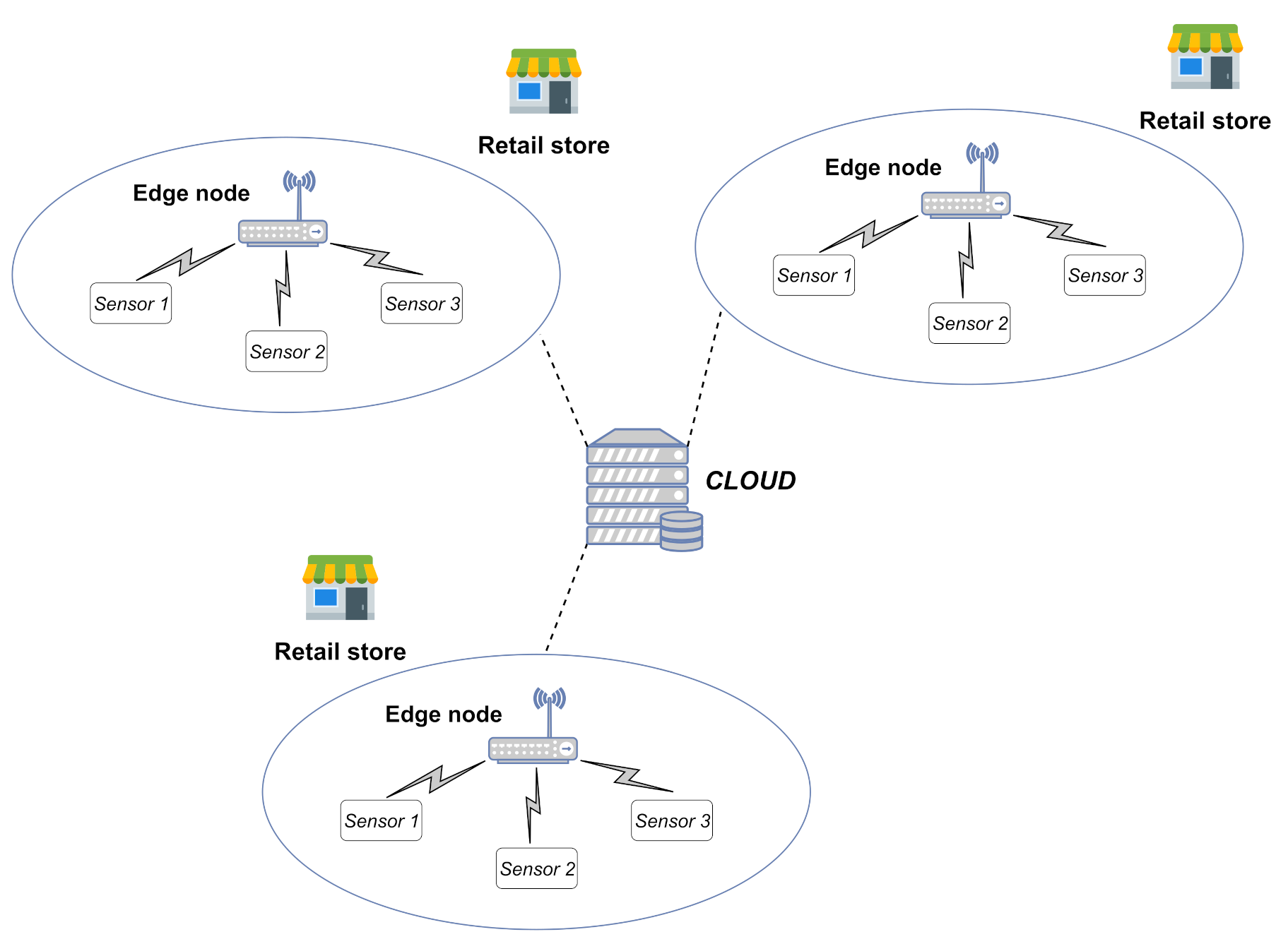
In this regard, the deployment of a data collection system to monitor indoor CO2 and IAQ represents a priority, especially in crowded environments such as tertiary buildings (i.e., retail stores, supermarkets and bank branches). A common approach to this consists of smart Internet of Things (IoT) sensors sensing the environment and communicating (through a wide range of possible protocols, e.g., Modbus [4], Wi-Fi [5] and EnOcean [6]) with an edge device which collects and processes the data. Moreover, in complex architectures the edge node could also play the role of gateway towards the network infrastructure. A typical scenario is that of retail stores, depicted in Figure 1, where managers aim to guarantee the best possible environmental conditions within their sites to make customers feel comfortable, hence encouraging them to shop.
Although the monitoring of real-time CO2 through smart IoT sensors can give important benefits in this direction, such an approach does not provide any information on the future behavior of CO2. This is a major limitation, as forecasting CO2 is crucial for applying preventive actions, e.g., by means of intelligent systems capable of automatically regulating HVAC devices in advance. Thanks to the increasing interest for IAQ, over the last decade a number of studies regarding the forecast of indoor CO2 have been published [7,8,9,10,11,12,13,14]. The proposed solutions mainly focus on maximizing the CO2 prediction accuracy by means of different artificial intelligence (AI) techniques.
Despite the promising results, a pure performance-oriented approach (i.e., which mainly focuses on prediction accuracy) might limit the applicability of such solutions in real-world scenarios. Indeed, the maximization of the performance is typically achieved by using a significant amount of data collected over a long time period [7,8,9,10] or by leveraging on complex input variables from expensive cutting-edge sensors [9,11]. In this regard, such a scenario requires data collection for many days, even months, for training the artificial intelligence models. As a result, managers of retail stores have to wait a long time before the full deployment of the system, making it unattractive from a business point of view. Moreover, to the best of our knowledge, none of the state-of-the-art solutions tackle the challenges of periodically updating the model to deal with the changes of the monitored environment (e.g., unusual behaviors of CO2 due to changes in human activity).
In this work, we propose a practical approach for predicting indoor CO2 using a limited window of indoor environmental data (i.e., temperature, humidity and CO2) collected over a short time frame to train neural network models. It achieves comparable accuracy of predictions with state-of-the-art solutions. The designed approach not only enables the CO2 predictions to be made very shortly after the beginning of the data collection (i.e., after just one day), but in the first period of the system’s deployment, the model can progressively learn new features by increasing the window of data day by day. As a result, the model is constantly updated and the performance is improved as soon as possible. Once the window achieves the optimal size to guarantee high prediction accuracy, it can be moved at a certain rate over time to update the model, effectively becoming a mobile window. As the training can be directly performed on site, the result is a potential zero-touch approach for predicting indoor CO2, enabling the edge device to work independently. Starting from a prediction error between 40 and 50 ppm after one day of data collection, the proposed approach improves the accuracy day by day. In particular, after just a week of data for training the model, the prediction error is more than halved, making it around 15 ppm, and predictions could be effectively used to regulate HVAC systems accurately. The performance improves until a window of past 30 days is used: in this case, an error of predictions of around 10 ppm is achieved. Further increasing the mobile window does not improve the accuracy and requires more computational resources.
Combining the practical constraints of real-world deployments with the requirement of accurate CO2 predictions, this work makes the following contributions:
- A deep learning solution for indoor CO2 prediction that can be trained with just a small amount of recent environmental data (i.e., temperature, humidity and CO2) collected over a short time frame, thereby guaranteeing a high prediction accuracy after few days from the beginning of the data collection with no model pre-training.
- An updating mechanism based on a mobile window that keeps the CO2 predictions consistent with any environmental changes. As a result, the CO2 predictions can be effectively used to regulate HVAC systems, guaranteeing IAQ comfort to occupants.
The rest of the paper is organized as follows. Section 2 provides a detailed overview of the relevant literature. Section 3 introduces the dataset used for the experimental evaluation. Section 4 describes the proposed methodology and the AI architecture. Section 5 illustrates the simulation setup. Section 6 describes and discusses the results of the proposed approach. Finally, Section 7 concludes the paper and provides future directions for predicting IAQ.
2. Related Work
In [14], the authors evaluated the use of relative humidity and temperature for modeling indoor CO2 by means of a multilayer perceptron (MLP), aiming to avoid deploying expensive CO2 sensors. Although data collected over six months were considered and advanced statistical features (e.g., kurtosis, skewness) were extracted from data to get as much information as possible to train the model, the performance was poor, and the same authors underlined the need for additional input variables. As a result, the following studies focused on adding new input variables. For example, in [7] the outdoor temperature and humidity—and other different parameters, such as the date and time—were introduced to predict CO2 using random forest, taking into account different training dataset sizes and numbers of trees. In this case, better performance was achieved, but a large dataset covering more than a year was used for training.
Unlike the previous studies, the historical data of CO2 and time parameters, such as weekday, hour and minute, were integrated within the study provided by [8]. Two different scenarios were analyzed using an ANN with three hidden layers: the first case considered all input variables, including the time information, and the second case only focused on the historical data of CO2. The results show that the time and date variables do not contribute to improving the accuracy of predictions. Moreover, the chosen approach relies on a large amount of data (corresponding to a time window of 242 days) to train the model. The evaluation was limited to just 10 h of the day after the training time window. A similar scenario considering only CO2 data as the input variable was evaluated in [12]. In this case, the authors took into account CO2 values with a time granularity equal to one hour, bounding the analysis to only working hours. The proposed neural network was trained using the data of a week (from Monday to Friday, excluding the night period), and CO2 values of next Monday and Tuesday were predicted. Although the results proved a good correlation between the true and predicted values using a small amount of data for training the neural network, this study was affected by clear limitations: only a couple of days were considered for the test, thereby restricting the performance overview of the proposed method, and a large time granularity (i.e., 1 h) of data was used. A deep analysis regarding the benefits of using CO2 as an input variable was provided by Khazaei et al. [13]. Three different approaches were considered: the first case included CO2 as the input variable; the second case only took into account humidity and indoor temperature; and the third case partially used CO2 as the input variable to evaluate predictions five time-steps in the future. All these cases correspond to different ways of training the neural network (in this case, MLP). Similarly to in [14], the authors highlighted the importance of collecting CO2 data through sensors to be used in the model training. Despite the use of a small amount of data for training the model and the good prediction accuracy, a limited scenario given by just a week of data was evaluated as in [8,12]. Furthermore, all the above studies did not consider updating of the models over time.
In the literature, some studies included the prediction of CO2 as a part of the forecast of IAQ in general. Unlike the previous works, they also considered different neural network architectures for forecasting IAQ. For example, in [11] the authors estimated and predicted CO2 and particulate matter (PM) 2.5 in some university classrooms through an optimized long short term memory (LSTM) model. Despite the good prediction accuracy, they took into account detailed variables (e.g., indoor NO2, wind speed, wind direction and number of students) which need cutting-edge sensors, making the whole data collection system to predict indoor CO2 expensive. Similarly, in [9], the authors used a gated recurrent unit (GRU) network as deep learning technique to predict fine dust, light amount, volatile organic compound (VOC), CO2, temperature and humidity by giving the past values of the same variables as input to the neural network. However, the architecture proved to be very heavy: it requires more than a day and a half to be trained, resulting in an inefficient solution to be used on edge devices. Moreover, data collected over more than six months and complex variables were considered.
In this work we mainly refer to [10]. Unlike all the above studies, it provides a detailed overview of the prediction of indoor CO2, starting from the data collection architecture to the forecast results of the models, taking into account the challenges of using edge devices in such a problem. In this work, different artificial intelligence techniques (ridge, decision tree, random forest, multilayer perceptron) were analyzed from both a computational load and a prediction accuracy point of view. Moreover, the impacts of the input variables and the number of past values to use, along with the number of future values to predict, were evaluated. Due to their computational load, the authors underlined the infeasibility of applying neural networks on edge devices to address this issue. As a result, a less computationally demanding technique, such as a decision tree, was suggested. Despite the detailed analysis, the proposed approach may be difficult to be applied in a real scenario. Indeed, a large amount of data collected over a whole year from different rooms was taken into account to train models for predicting CO2 within the monitored rooms in the so-called “hard sections” (i.e., when CO2 has a significant variation). As a result, it is necessary to collect data for a long time period before training the AI models.
Table 1 highlights the key points of each work presented in this Section. Compared to them, a major benefit of our approach is the automated updating mechanism, which is necessary to keep up with the changes in the environmental conditions, and hence to cope with the dynamics of real-world application scenarios.
3. Dataset
In this work we used the data provided and published by Kallio J. et al. [10]. As reported by the authors, this dataset has been published for further analysis of CO2 predictions; thus, it is suitable for our objectives. It consists of data collected from 13 different rooms, including offices and meeting rooms, by means of different commercial sensors at Technical Research Center of Finland (VTT) in 2019. The monitored variables are:
- Temperature [°C];
- Relative humidity [%];
- Air pressure [hPa];
- Carbon dioxide concentration [ppm];
- Activity level.
We pre-processed the data by using a script developed by Kallio J. et al. [10], which automatically aligns the timestamps of sensor data collected from the same room. As underlined by Kallio J. et al. in their paper, the sensors of five rooms were affected by communication issues during the data collection, leading to more than 10% of samples being incomplete (i.e., missing at least one between T, H or CO2). The script fixed that issue by filling each gap with the mean between the previous value and next value. The script also implements methods to split the dataset into training and testing data. We did not use this functionality, as we found out that during the split process the script excludes the periods of time with slow variations of CO2. This would prevent the validation of our solution in every condition. Instead, we implemented a custom method to split the data within a given mobile window into a training set (70%) and validation set (30%) (as indicated in Section 5). As described in Section 4, we tested the prediction on the first day after the time window.
4. Methodology
4.1. Neural Network Architecture
A 1-dimensional convolutional neural network (CNN) was used as the deep learning architecture. 1D CNNs, which find applications in natural language processing (NLP) [15], in network security [16] and in other domains, are able to automatically analyze and extract features from a single spatial dimension (in our case, time) by means of convolution operations [17], hence learning in-depth patterns among data. From a computational point of view, they guarantee good performance by using a shallow structure and advanced features, such as weight sharing, and have the possibility of using a small amount of data for training the model [18] without significantly impacting the accuracy. Unlike other types of neural networks (e.g., recurrent neural networks) proposed in the literature [9,11], 1D CNNs are less computationally demanding [19], making them suitable for limited-power and resource-constrained devices.
The neural network architecture was developed using Keras [20], the framework built on TensorFlow platform (version 2.4.0), and Python (version 3.7.3), following specific guidelines to adapt 1D CNN for time-series forecasting [21].
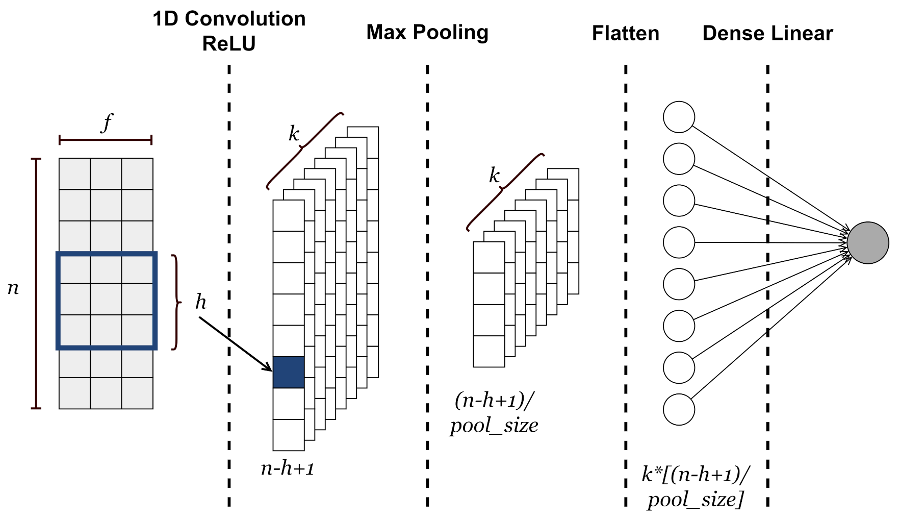
The proposed CNN architecture, depicted in Figure 2, consists of the following layers:
- Input layer. A sample consists of the values of the input environmental variables (i.e., temperature, humidity and CO2) covering a window of n quarters of an hour. Basically, a sample is a data matrix of size , where n is the number of quarters of an hour and f is the number of features. This kind of approach is possible due to the temporal nature of environmental variables. Indeed, the values of temperature, humidity or CO2 at close time intervals are correlated with each other. Before feeding the neural network, the input values are normalized by defining a maximum and minimum value for each variable.
- 1D Convolutional Layer. It is devoted to analyzing and extracting features along the time-dimensional axis of the input data. This layer outputs a matrix of size in which each column is a feature vector extracted through so-called convolutional filters or kernels. Each of these k kernels slides over the input matrix with a step equal to 1 and performs a convolution operation to extract the most significant local information. The common rectified linear activation function (i.e., ReLU(x) = max{0,x}) is used to extract non-linearity patterns from data.
- Max Pooling layer. It aims to learn most valuable information from extracted feature vectors by applying a subsampling operation to the output matrix from the CNN layer. This operation involves a filter that slides along each feature map according to a step given by the stride parameter and applies a maximum operation to a number of elements equal to the pool size parameter. In this case, the stride is set equal to pool size. A matrix of is obtained as output.
- Flatten layer. It reshapes the input matrix to provide a one-dimensional feature vector which can be used to make predictions by the output layer.
- Output layer. This linear fully connected layer, whose output consists of a single neuron, predicts the CO2 value for the next quarter hour.
4.2. Proposed Approach
The proposed approach is based on the use of a small amount of data collected over a short time frame for training the neural network models. As a result, the proposed system is able to be operative and provide accurate predictions a short time after its initial deployment, without the need for collecting large amounts of data over many days or from other environments to achieve high accuracy of predictions. In this regard, we introduce the concept of the mobile window, which refers to the amount of recent data used to train and update the model over time. It relies on the idea that only the recent data involve valuable information with which to model the local environment in the future. On the contrary, including old data collected during far in the past would likely degrade the accuracy of the predictions, as data might include behaviors related, e.g., to a another season of the year. As a result, the mobile window represents a dynamic mechanism to keep the model up to date upon recent environmental changes. The mobile window size is tuned to achieve a prediction accuracy in the range of 10–20 ppm to guarantee accurate regulation of the HVAC, according to the results of previous studies [10]. The proposed approach can be easily integrated among the typical data collection operations for monitoring IAQ. Moreover, thanks to the use of a small amount of data and the design of a lightweight neural network architecture (i.e., 1D CNN), such an approach can be effectively applied on edge devices to forecast the local CO2 level with complete autonomy, resulting in a potential zero-touch indoor CO2 prediction approach.
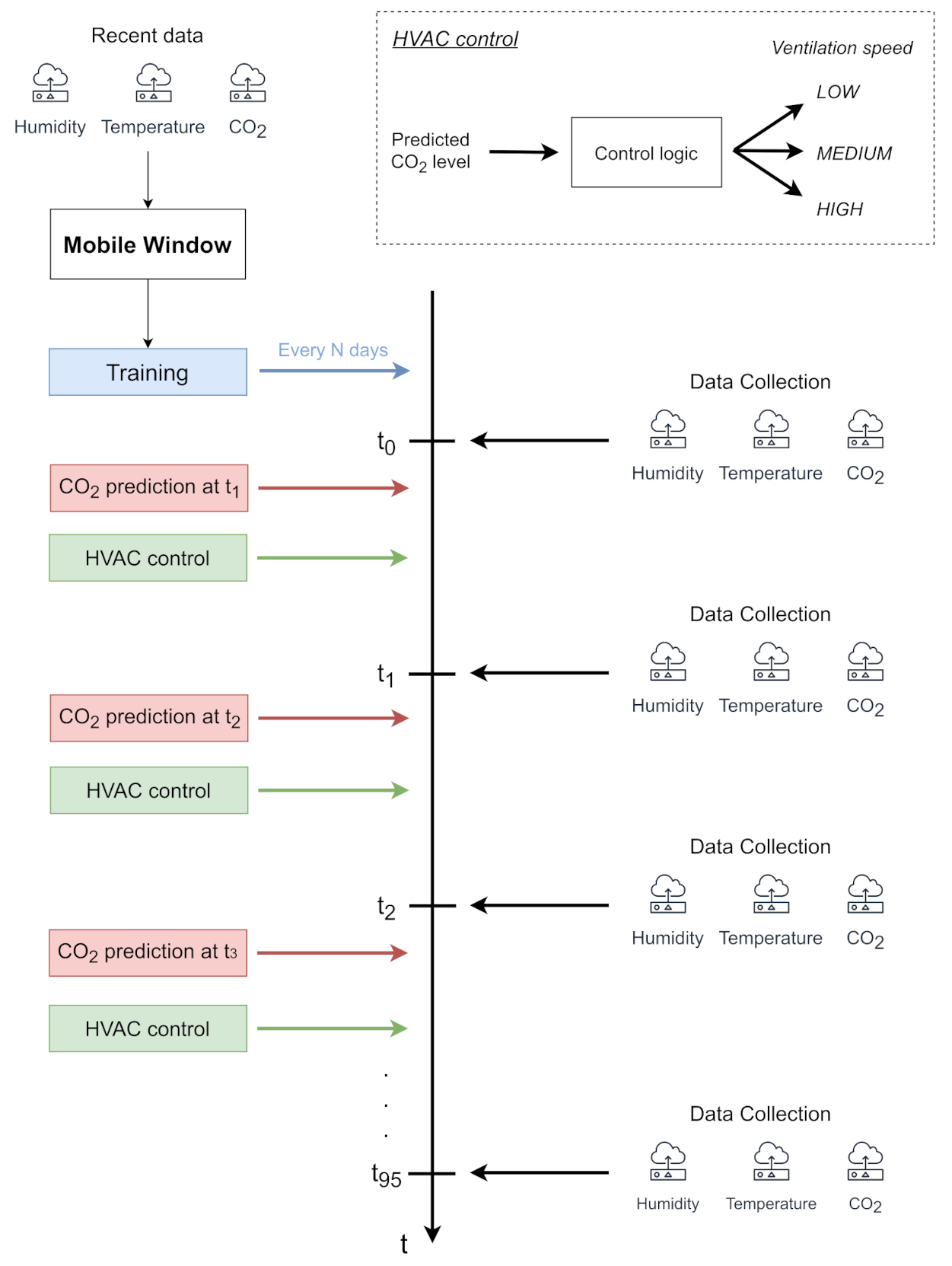
The main operations of our approach can be summarized as follows (Figure 3):
- Every quarter of an hour of the day t0, t1, …, t95, the environmental data (i.e., temperature, humidity, CO2) are collected on the edge device through smart IoT sensors. Indeed, collecting data every 15 min guarantees a good trade-off among the accuracy of analysis, battery lifetime of sensors and storage capabilities of the edge device. Moreover, some industrial protocols, such as Modbus, keep the channel busy during their reading operations. A quarter-hour granularity avoids occupying the physical channel at a high rate as well, enabling the edge device to perform other local operations (e.g., actuation and energy data monitoring) without potential interference.
- Immediately after the data collection, every quarter of an hour, t0, t1, …, t95, the system handles the collected data as samples. In particular, the sample, including the values of the environmental variables of the last n quarters of an hour, is given to the convolutional neural network to predict the CO2 level of the next quarter hour. In this way, the forecast value of CO2 for the next future is regularly provided, taking into account the behavior of the environmental variables in the last short period. The predicted value can be effectively used to regulate HVAC systems in advance in order to keep the CO2 level under control.
- Every N days, a window of data collected over the last few days is used to update the neural network model. In the first period of the deployment, this window progressively increases to account for a larger amount of information to improve the modeling of the environmental variables. As a result, the proposed approach guarantees the improvement of the performance as soon as possible. Once the window achieves its optimal size as the trade-off between the prediction accuracy and computational demand, it slides over time to update the models, effectively becoming a mobile window. From a processing point of view, the data are handled as samples, which are then used to feed the 1D convolutional neural network for training the model. This operation can be properly scheduled after the last data collection operation of the day (before t0).
5. Simulation Setup
Table 2 reports the values of the main parameters used in the simulations.
Temperature, humidity and CO2 of the dataset were used as input variables to predict future CO2 levels. They are the most relevant variables required to be monitored by managers to have an overview of IAQ. Additional cutting-edge sensors to monitor complex air pollutants, such as particulate matter (PM1, PM2.5 or PM10) or VOC, make the cost of a data collection system increase significantly. Moreover, these variables depend not only on human activity but also on other agents, which can be considered of minor interest in a scenario such as that of retail sites. As a result, we optimized the choice of the input variables, coherently with the rest of the proposed system. Their value ranges are reported in Table 3.
In [10], the data were characterized by a time granularity equal to one minute. However, the original values of the dataset were aggregated every 15 min in order to simulate a typical data collection scenario.
We evaluated the main hyper-parameters of the 1D CNN in order to find the values to guarantee a good trade-off between the accuracy of the model and its computational requirements. In this regard, we used root mean squared error (RMSE) as the performance metric:
where yi is the real CO2, is the predicted CO2 and N is the total number of quarters of an hour.
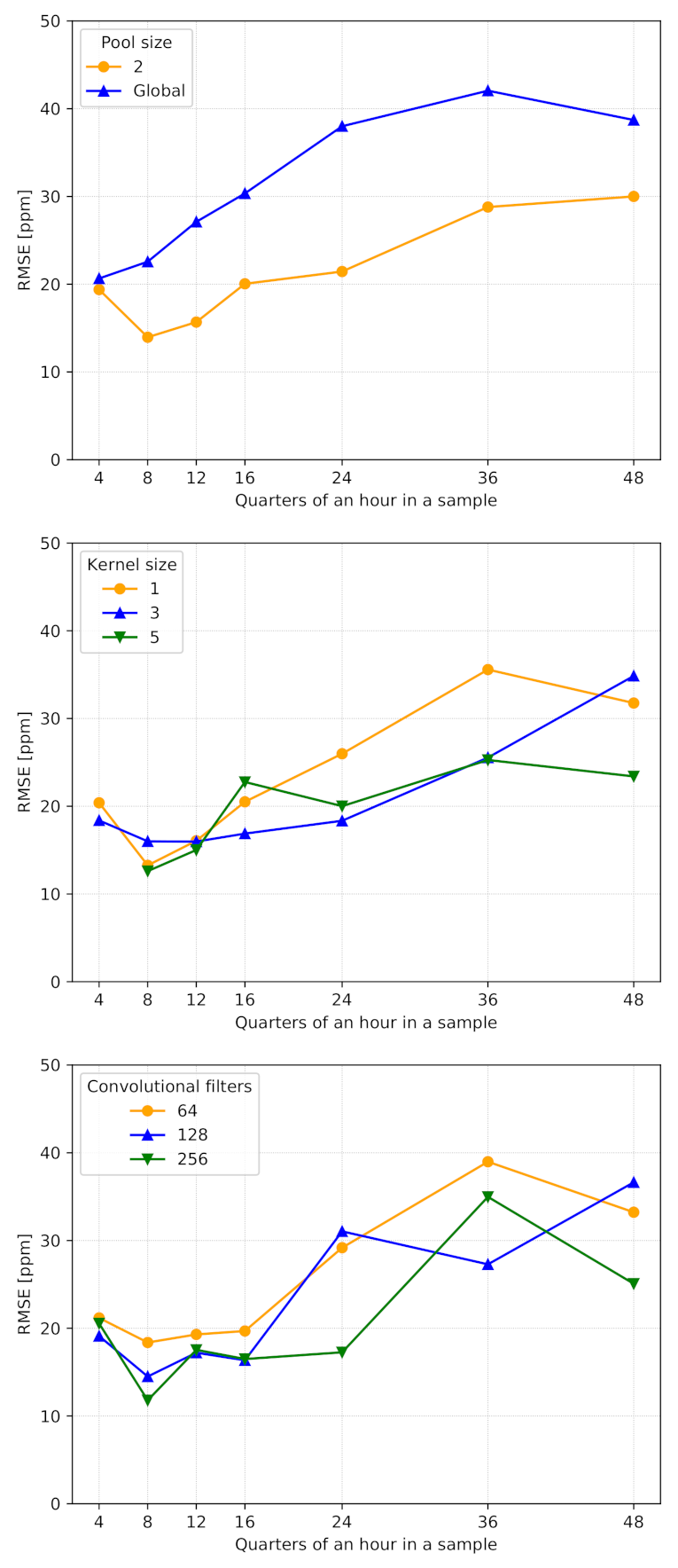
We evaluated the performance of the system by varying the number of quarters of an hour per sample. We experimented by considering other relevant parameters—such as pool size, kernel size and number of convolutional filters—and report the results in Figure 4:
- Pool size is important to extract the most relevant information from the feature vectors provided by the convolutional layer. According to Figure 4, we set it equal to 2, as global max pooling impacted the accuracy significantly.
- Kernel size has a central role in extracting valuable information along the time dimension. The simulation results reported in Figure 4 show similar performances between different kernel sizes. Thus, we set it equal to 3, which is one of the standard values for CNNs.
- Number of convolutional filters was set to 64. Indeed, as reported in Figure 4, we noticed that higher values (e.g., 128 and 256) guaranteed similar performances, especially when samples included a few quarter-hour measurements. In this way, we provide more compact and lightweight models, reducing their memory footprints and guaranteeing faster computation, especially on limited-power and resource-constrained devices.
Other parameters were:
- The learning rate was set to 0.001, a value used in many complex and non-linear problems, which guarantees a good trade-off between convergence and computational time.
- The batch size was set to 32 to guarantee stability, and to limit the memory footprints of the models.
- Adam optimizer [22] was used as the optimization algorithm.
- RMSE was used as the loss function during the training.
- The validation split was set to 0.3, as per common practice in studies on CO2 prediction. Before the split, we shuffled the samples so that both training and validation sets contained samples which were spread across the whole time window. Please note that we did not shuffle the time series within a single sample, as we wanted to preserve the chronological order of the consecutive quarters of hour.
- The maximum number of epochs was set to 5000, alongside an early stopping patience parameter set to 25 epochs.
6. Results and Discussion
In order to evaluate our proposed system, we defined a couple of experiments, in particular:
- 1.
- The first experiment aimed to understand the impact of the mobile window, aiming to highlight the practical and adaptive features of the proposed approach;
- 2.
- The second test evaluated the performance when more days in the future were predicted in order to simulate a model update after N days.
6.1. Mobile Window
The most important hyper-parameter of the proposed approach is the mobile window, i.e., the amount of data used to train the models, which needs to be deeply investigated in order to understand how its size affects the accuracy of the predictions.
For this analysis, we used the simulation setup analyzed in the previous section. Given a certain mobile window of N days, for each of the 13 rooms of the dataset, we picked one random day per month to predict using the previous N days for training. Finally, we averaged all the results to get the overall performance for a certain size of mobile window. This experimental approach enabled us to simulate our methodology while taking into account any possible period of the year (i.e., the deployment of the proposed system at any time of the year) and environments with different physical characteristics (i.e., volume and area), thereby providing a detailed overview of the performance of the proposed approach, unlike previous research (e.g., [8,12,13]). As reported in Section 3, the dataset is affected by some missing values due to communication failures during the data collection. As this issue could have impacted the correctness of the predictions, we excluded from our experiments those days with holes in their data, and those days that would have otherwise been included in the previous N days used for training.
The experiment was executed on Raspberry Pi 4 Model B with 4 GB of memory, which played the role of edge device.
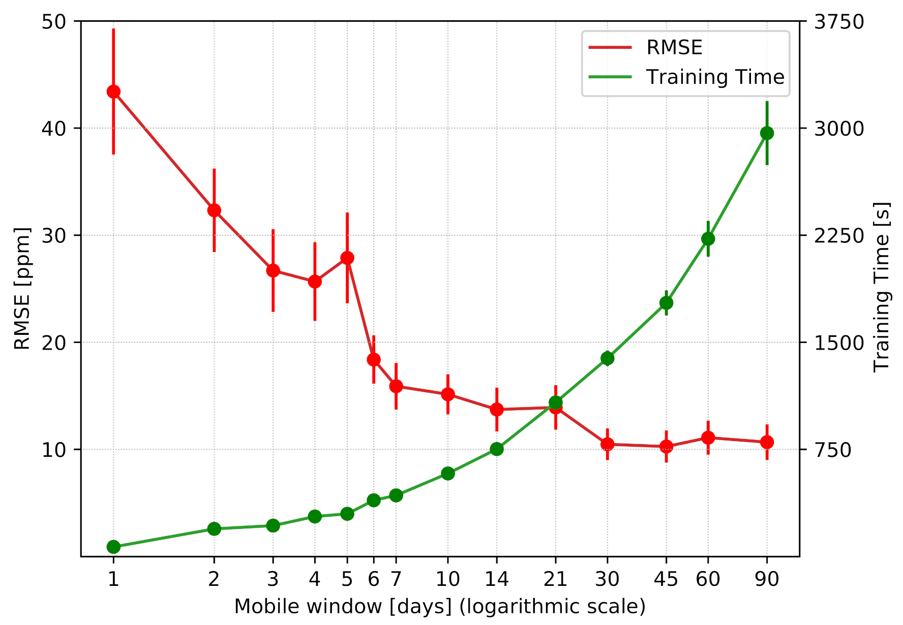
Figure 5 outlines the results of this experiment, demonstrating the benefits of the proposed approach. In the first place, it underlines the feasibility of deploying the system after just one day of data collection, without the need for any pre-training or gathering of a large amount of data. Despite poor performance in the first days due to a low correlation between the days included in the mobile window and the day to predict, the accuracy dramatically improved in a few days. Indeed, the model was able to progressively learn complex features, improving the modeling of the indoor environmental behavior. In terms of numerical results, after just a week, the RMSE became about 15 ppm, guaranteeing high accuracy for regulating HVAC systems. As a result, in the first period of deployment, the model can be regularly updated, progressively increasing the mobile window used for the training in order to improve the performance as soon as possible from the beginning of data collection.
The plot in the figure also shows that mobile windows larger than 30 days did not bring any major improvements in terms of RMSE. On the other hand, as the training time grows exponentially, a short time window is preferred to avoid overloading the edge node and to minimize the impacts on other (critical) processes that might be executed on the same device.
The results of this experiment highlight the benefits behind the proposed approach:
- 1.
- In the first period of the system deployment, the performance can be progressively improved by introducing more data in the mobile window.
- 2.
- After only a month of data collection, the proposed approach guarantees the best performance in terms of prediction accuracy.
- 3.
- A window of data including the last 30 days can be effectively moved over time to freshen the model at a certain rate, effectively becoming a mobile window.
Moreover, with a time window size of 30 days, the model took about 25 min to train. Thus, this operation can be scheduled when the device is idle or does not execute critical operations (e.g., overnight, when the retail store is closed). Therefore, according to the above considerations, we can conclude that a 30-day mobile window allows a good trade-off between computational demand and accuracy.
Nevertheless, the proposed approach is affected by some limitations. First, the RMSE during the first week was above the target threshold of 10–20 ppm. Although the performance of the system improved quickly, this warm-up phase could possibly lead to non-optimal regulations of HVAC systems. Second, the current version of the system is not resilient to missing values, as it requires a robust data collection system to work properly. This means that in cases of holes in the data (because of, e.g., communication issues or sensor failures), the future level of CO2 cannot be predicted. In this regard, for further improvement of the system, we plan to solve this issue by implementing a mechanism that finds the largest time window with no holes in the past data, which would be used to perform the predictions of the CO2 level. Here the challenge will be to find a trade-off between the size and the age of the old window. Thus, we need a sufficiently large time window for a good prediction, but we do not want to go too far into the past to find such a large time window.
6.2. Model Update Rate
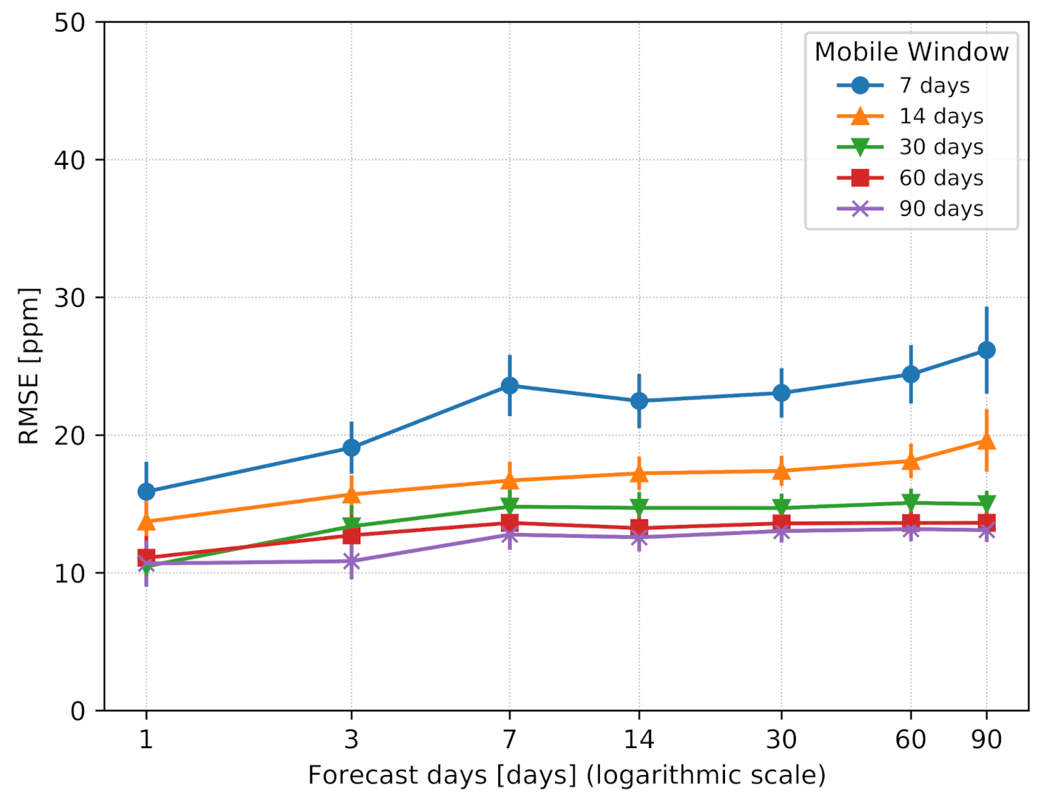
According to the previous analysis, the model can be effectively updated every day. However, it is reasonable to wonder whether the model update rate can be softened once the size of the mobile window achieves the desired size, and thus how often the model should be re-trained to maintain the desired level of accuracy. To that end, we set the window size to a given value, and we evaluated the prediction error of our model when increasing the number of forecast days.
Figure 6 reports the results of this experiment. They outline how the prediction error increased very slowly as the number of future days to predict increased. This means that the indoor environmental behavior did not change in a significant way over the weeks, proving once again that using large amounts of data over many days do not provide significant benefits for predicting indoor CO2. Such a result enables the system to potentially update the model at a slower rate with respect to every day. For example, the model could be effectively refreshed once a week in a retail store, during the weekend when the store may be closed, and the edge device would be idle most of the time. However, the best performance in terms of accuracy is guaranteed with daily updating of the model, which can be properly scheduled for the end of the day, as defined by the previous experiment of the mobile window, when all the data of the previous N days are collected on the edge device.
7. Conclusions
In this paper, we have presented a practical approach for indoor CO2 prediction. In particular, we have introduced a deep learning solution based on a dynamic mobile window that allows system deployment with no pre-training of the AI model, and an adaptive mechanism to keep the model up to date upon environmental changes. The proposed approach guarantees high performance in a short time frame after the initial deployment and automatically tunes the size of the mobile window until the best settings are reached. The predictions can be effectively used to regulate HVAC systems in advance in order to avoid high levels of CO2, hence guaranteeing high levels of comfort on site.
Evaluation results show that the proposed system can be effectively executed on edge devices, resulting in a potential zero-touch approach for indoor CO2 prediction. It is worth noting that with our solution, each edge device relies only on its own collected data to update the model and to predict the future CO2 level, making the system setup and its general operation more practical in a real-world scenario.
Author Contributions
Conceptualization, G.S., C.P. and D.S.; methodology, G.S., R.D.-C. and D.S.; software, G.S.; validation, G.S., R.D.-C. and D.S.; formal analysis, G.S., R.D.-C. and D.S.; investigation, G.S., R.D.-C. and D.S.; resources, G.S.; data curation, G.S., R.D.-C. and D.S.; writing—original draft preparation, G.S.; writing—review and editing, G.S., R.D.-C. and D.S.; visualization, G.S. and C.P.; supervision, C.P. and D.S.; project administration, T.G. and D.S.; funding acquisition, C.P. and T.G. All authors have read and agreed to the published version of the manuscript.
Funding
The work in this paper has been partially funded by “Programma operativo FESR 2014–2020” of Provincia autonoma di Trento, with co-financing of European ERDP funds, through project “GEM-Retail” and by the European Union’s Horizon 2020 Research and Innovation Programme under grant agreement no. 872548 (DIH4CPS: Fostering DIHs for Embedding Interoperability in Cyber-Physical Systems of European SMEs).
Institutional Review Board Statement
Not applicable.
Informed Consent Statement
Not applicable.
Data Availability Statement
Conflicts of Interest
The authors declare no conflict of interest. The funders had no role in the design of the study; in the collection, analyses, or interpretation of data; in the writing of the manuscript, or in the decision to publish the results.
References
- Satish, U.; Mendell, M.J.; Shekhar, K. Is CO2 an indoor pollutant? Direct effects of low-to-moderate CO2 concentrations on human decision-making performance. Environ. Health Perspect 2012, 120, 1671–1677. [Google Scholar] [CrossRef] [Green Version]
- Peng, Z.; Jimenez, J.L. Exhaled CO2 as a COVID-19 Infection Risk Proxy for Different Indoor Environments and Activities. Environ. Sci. Technol. Lett. 2021, 8, 392–397. [Google Scholar] [CrossRef]
- Join Research Center (JRC) of the European Commission. Available online: https://susproc.jrc.ec.europa.eu/ (accessed on 16 May 2021).
- The Modbus Organization. Available online: https://modbus.org/ (accessed on 13 July 2021).
- Wi-Fi Alliance. Available online: https://www.wi-fi.org/ (accessed on 13 July 2021).
- Energy Harvesting Wireless Sensor Solutions and Networks from EnOcean. Available online: https://www.enocean.com/ (accessed on 13 July 2021).
- Vanus, J.; Martinek, R.; Bilik, P.; Zidek, J.; Dohnalek, P.; Gajdos, P. New method for accurate prediction of CO2 in the smart home. In Proceedings of the 2016 IEEE International Instrumentation and Measurement Technology Conference Proceedings, Taipei, Taiwan, 23–26 May 2016; pp. 1–5. [Google Scholar]
- Khorram, M.; Faria, P.; Abrishambaf, O.; Vale, Z.; Soares, J. CO2 Concentration Forecasting in an Office Using Artificial Neural Network. In Proceedings of the 2019 20th International Conference on Intelligent System Application to Power Systems (ISAP), New Delhi, India, 10–14 December 2019; pp. 1–6. [Google Scholar]
- Ahn, J.; Shin, D.; Kim, K.; Yang, J. Indoor Air Quality Analysis Using Deep Learning with Sensor Data. Sensors 2017, 17, 2476. [Google Scholar] [CrossRef] [PubMed] [Green Version]
- Kallio, J.; Tervonen, J.; Räsänen, P.; Mäkynen, R.; Koivusaari, J.; Peltola, J. Forecasting office indoor CO2 concentration using machine learning with a one-year dataset. Build. Environ. 2021, 187, 107409. [Google Scholar] [CrossRef]
- Sharma, P.K.; Mondal, A.; Jaiswal, S.; Saha, M.; Nandi, S.; De, T.; Saha, S. IndoAirSense: A framework for indoor air quality estimation and forecasting. Atmos. Pollut. Res. 2020, 12, 10–22. [Google Scholar] [CrossRef]
- Putra, J.C.; Safrilah, S.; Ihsan, M. The prediction of indoor air quality in office room using artificial neural network. AIP Conf. Proc. 2018, 1977, 020040. [Google Scholar]
- Khazaei, B.; Shiehbeigi, A.; Kani, A.H.M.A. Modeling indoor air carbon dioxide concentration using artificial neural network. Int. J. Environ. Sci. Technol. 2019, 16, 729–736. [Google Scholar] [CrossRef]
- Skön, J.; Johansson, M.; Raatikainen, M.; Leiviskä, K.; Kolehmainen, M. Modelling indoor air carbon dioxide (CO2) concentration using neural network. Int. J. Environ. Chem. Ecol. Geol. Geophys. Eng. World Acad. Sci. Eng. Technol. 2012, 61, 37–41. [Google Scholar]
- Kim, Y. Convolutional Neural Networks for Sentence Classification. In Proceedings of the 2014 Conference on Empirical Methods in Natural Language Processing (EMNLP), Doha, Qatar, 21 October 2014; pp. 1746–1751. [Google Scholar]
- Doriguzzi-Corin, R.; Millar, S.; Scott-Hayward, S.; Martinez-del-Rincon, J.; Siracusa, D. LUCID: A Practical, Lightweight Deep Learning Solution for DDoS Attack Detection. IEEE Trans. Netw. Serv. Manag. 2020, 17, 876–889. [Google Scholar] [CrossRef] [Green Version]
- Albawi, S.; Mohammed, T.A.; Al-Zawi, S. Understanding of a convolutional neural network. In Proceedings of the 2017 International Conference on Engineering and Technology (ICET), Antalya, Turkey, 21–23 August 2017; pp. 1–6. [Google Scholar]
- Kiranyaz, S.; Ince, T.; Abdeljaber, O.; Avci, O.; Gabbouj, M. 1-D Convolutional Neural Networks for Signal Processing Applications. In Proceedings of the ICASSP 2019—2019 IEEE International Conference on Acoustics, Speech and Signal Processing (ICASSP), Brighton, UK, 12–17 May 2019; pp. 8360–8364. [Google Scholar]
- Lara-Benítez, P.; Carranza-García, M.; Riquelme, J. An Experimental Review on Deep Learning Architectures for Time Series Forecasting. Int. J. Neural Syst. 2020, 31. [Google Scholar] [CrossRef] [PubMed]
- Keras: The Python Deep Learning API. Available online: https://keras.io/ (accessed on 11 July 2021).
- How to Develop Convolutional Neural Network Models for Time Series Forecasting. Available online: https://machinelearningmastery.com/how-to-develop-convolutional-neural-network-models-for-time-series-forecasting/ (accessed on 11 July 2021).
- Kingma, D.; Ba, J. Adam: A Method for Stochastic Optimization. In Proceedings of the International Conference on Learning Representations, San Diego, CA, USA, 7–9 May 2015. [Google Scholar]
Figure 1.
A typical data collection scenario for retail stores.

Figure 2.
The designed neural network architecture.

Figure 3.
The sequence of operations at different quarters of an hour (t0, t1, …, t95) during a day.
Figure 3.
The sequence of operations at different quarters of an hour (t0, t1, …, t95) during a day.

Figure 4.
Behavior of the model with different numbers of quarters of an hour per sample, with a focus on the pool size value (top), kernel size value (center) and number of convolutional filters (bottom).
Figure 4.
Behavior of the model with different numbers of quarters of an hour per sample, with a focus on the pool size value (top), kernel size value (center) and number of convolutional filters (bottom).

Figure 5.
Behavior of RMSE and training time as the mobile window increases.

Figure 6.
RMSE as a function of the forecast days.


Table 1.
Summary of the SoA.
| Related Work | Dataset Size | Input Variables | AI Architecture | Automated Model Update |
|---|---|---|---|---|
| This Work | Adaptive (Max 30 days) | Temperature, Humidity, CO2 | 1D CNN | Yes |
| Vanus et al. [7] | One year | Temperature, humidity, time, date | Random Forest | No |
| Khorram et al. [8] | 242 days | CO2, weekday, hour, minute | ANN | No |
| Ahn et al. [9] | Six months | Fine dust, light amount, VOC, CO2, temperature and humidity | GRU | No |
| Kallio et al. [10] | One year | CO2, PIR, temperature and humidity | Ridge, Decision Tree, Random Forest, MLP | No |
| Sharma et al. [11] | One week | Indoor NO2, wind speed, wind direction, number of student | LSTM | No |
| Putra et al. [12] | One week | CO2 | ANN | No |
| Khazaei et al. [13] | One week | CO2, humidity, temperature | MLP | No |
| Skön et al. [14] | Six months | Temperature, humidity | MLP | No |
Table 2.
Simulation parameters.
| Parameter | Value |
|---|---|
| Environmental variables in input | Temperature, humidity, CO2 |
| Time granularity of data | 15 min |
| Quarters of an hour in a sample | 8 |
| Number of kernel filters—Convolutional layer | 64 |
| Kernel size—Convolutional layer | 3 |
| Pool size—Max Pooling layer | 2 |
| Learning rate | 0.001 |
| Batch size | 32 |
| Optimizer | Adam |
| Loss function | Mean squared error |
| Validation split | 0.3 |
| Maximum number of epochs | 5000 |
| Patience | 25 |
Table 3.
Range of the input variables.
| Parameter | Range |
|---|---|
| Temperature | 0–40 °C |
| Humidity | 0–80 % |
| CO2 | 350–5000 ppm |
Publisher’s Note: MDPI stays neutral with regard to jurisdictional claims in published maps and institutional affiliations. |
© 2021 by the authors. Licensee MDPI, Basel, Switzerland. This article is an open access article distributed under the terms and conditions of the Creative Commons Attribution (CC BY) license (https://creativecommons.org/licenses/by/4.0/).
Share and Cite
MDPI and ACS Style
Segala, G.; Doriguzzi-Corin, R.; Peroni, C.; Gazzini, T.; Siracusa, D. A Practical and Adaptive Approach to Predicting Indoor CO2. Appl. Sci. 2021, 11, 10771. https://0-doi-org.brum.beds.ac.uk/10.3390/app112210771
AMA Style
Segala G, Doriguzzi-Corin R, Peroni C, Gazzini T, Siracusa D. A Practical and Adaptive Approach to Predicting Indoor CO2. Applied Sciences. 2021; 11(22):10771. https://0-doi-org.brum.beds.ac.uk/10.3390/app112210771
Chicago/Turabian StyleSegala, Giacomo, Roberto Doriguzzi-Corin, Claudio Peroni, Tommaso Gazzini, and Domenico Siracusa. 2021. "A Practical and Adaptive Approach to Predicting Indoor CO2" Applied Sciences 11, no. 22: 10771. https://0-doi-org.brum.beds.ac.uk/10.3390/app112210771
Note that from the first issue of 2016, this journal uses article numbers instead of page numbers. See further details here.