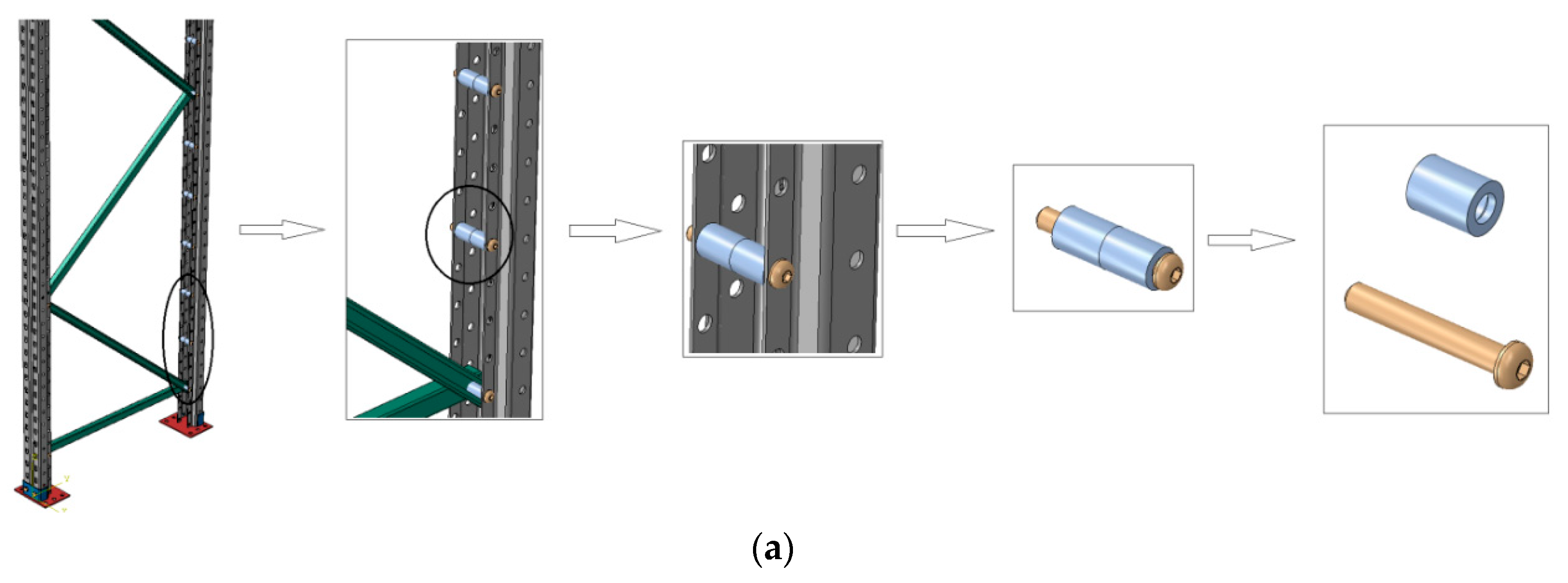
Article

Numerical Evaluation of the Upright Columns with Partial Reinforcement along with the Utilisation of Neural Networks with Combining Feature-Selection Method to Predict the Load and Displacement

1
Centre for Infrastructure Engineering, Western Sydney University, Kingswood, Sydney, NSW 2747, Australia
2
Department of Civil Engineering, K.N. Toosi University of Technology, Mirdamad, Tehran 1969764449, Iran
3
Department of Construction Engineering and Management, Amirkabir University of Technology, Tehran 1591634311, Iran
*
Authors to whom correspondence should be addressed.
Appl. Sci. 2021, 11(22), 11056; https://doi.org/10.3390/app112211056
Submission received: 21 September 2021 / Revised: 6 November 2021 / Accepted: 14 November 2021 / Published: 22 November 2021

Abstract

:
This study evaluated the axial capacity of cold-formed racking upright sections strengthened with an innovative reinforcement method by finite element modelling and artificial intelligence techniques. At the first stage, several specimens with different lengths, thicknesses and reinforcement spacings were modelled in ABAQUS. The finite element method (FEM) was employed to increase the available datasets and evaluate the proposed reinforcement method in different geometrical types of sections. The most influential factors on the axial strength were investigated using a feature-selection (FS) method within a multi-layer perceptron (MLP) algorithm. The MLP algorithm was developed by particle swarm optimization (PSO) and FEM results as input. In terms of accuracy evaluation, some of the rolling criteria including results showed that geometrical parameters have almost the same contribution in compression capacity and displacement of the specimens. According to the performance evaluation indexes, the best model was detected and specified in the paper and optimised by tuning other parameters of the algorithm. As a result, the normalised ultimate load and displacement were predicted successfully.

1. Introduction

Warehousing systems are widely used to manage industrial production. Since cold-formed steel (CFS) sections have been developed in racking systems, steel storage systems are extensively employed in various industries [1,2,3,4]. Uprights are critical components of the racking systems, which play the same role as a column in other structures. The stability of the racking systems directly depends on uprights where a combination of different failure modes is probable under service loads [5,6,7,8,9,10]. Since racking systems typically experience extreme loading scenarios, the design of the uprights has become a vital task [11,12,13,14,15,16].
The structural performance of the upright raking systems has been widely studied under different axial load scenarios. Koen [17] evaluated stub uprights to identify the effective length of the racking uprights under service loads by obtaining a set of reduction coefficients. Davies et al. [18] experimentally and numerically investigated failure modes of the stub uprights under compression. According to their study, limited tests are promising for designing racking uprights. According to Trouncer and Rasmussen’s study [19], the prediction of the capacity of uprights is more decisive by EN 15512 [20] specifications compared to Rack Manufacturers Institute (RMI). Gilbert and Rasmussen [21] performed general tests on racking systems to enhance EN 15512 specifications and presented some clarifications to determine in-plane stiffness.
The combination of different buckling modes in upright frame elements was studied in the form of research programs. Pedro et al. [22] evaluated the local-distortional buckling combination in fixed-end CFS uprights. Based on the concept of reduced thickness, the interaction of buckling along with short stiffened columns was examined by Roure et al. [23]. According to their reports, the typical design codes were inadequate, which means that the interaction of different failures and buckling should be calculated. Distortional buckling of upright columns was studied along different lengths and thicknesses by Casafont et al. [24] who finally derived a set of design configurations and equations for failure modes.
The finite element (FE) method as a reliable approach for the process of data prediction and validation is commonly conducted by FE programs such as ANSYS and ABAQUS. Using the relevant programs to evaluate the structural performances has been widely developed in recent years. Johns Hopkins University and Griffith University performed a series of optimisation tests on CFS cross-sections to achieve ‘global optimum’ solutions. Numerical evaluation of racking systems currently is a typical approach to derive the optimum values of CFS sections and upright characteristics. Two famous numerical approaches including finite strip method and direct strength method were conducted along the genetic algorithm (GA) [25,26] to obtain the best possible upright columns [27,28,29,30]. In this study, various lengths and thicknesses of cold-formed uprights were modelled by ABAQUS with different reinforcement distances.
Generally, artificial intelligence (AI) techniques are able to address some of the previous engineering issues due to their advantages compared to classic methods [31,32,33,34,35,36]. Learning and mocking are two significant points of AI, which make these algorithms favourable for researchers [37,38,39,40,41]. Employing optimisation techniques such as back-propagation algorithms [42], a raw model of artificial neural networks (ANNs) is generally developed. ANN can solve three types of problems including: (1) classification, (2) function-approximation and (3) time series prediction [43,44,45,46,47]. However, getting stuck in local extremums and difficulty in crossing plateaus of error function landscape are common defects of classic approaches [48,49,50,51,52]. In this regard, metaheuristic (MT) optimisation algorithms such as GA [53], particle swarm optimisation (PSO) [54] and imperialist competitive algorithm (ICA) [55] can be used to address mentioned drawbacks.
In some cases, the ANN performance can be improved by the global search feature of these methods. ANNs and some optimisation techniques have been recently applied for solving nonlinear and sophisticated engineering problems. One of the ANN developments is adaptive neuro-fuzzy inference system (ANFIS) that has become a trending algorithm for prediction [56]. In medical researches, ANFIS has also been conducted for predicting a number of verified patient cases [57,58]. A novel combination set of ANFIS was developed in China to predict the number of contaminated cases from COVID-19 [59]. Moreover, hybrid algorithms are typically employed to solve multiobjective problems [60,61]. Therefore, different types of optimisation methods can be integrated with ANFIS to increase the accuracy and improve the performance of the considered algorithm. The multi-verse optimiser (MVO) approach was combined with ANFIS to calculate the consumption of materials [62]. This hybrid algorithm is utilised to solve the consumption rate of material and predict that from a dataset that has been derived from different areas. The MLP neural network is suitable for prediction, especially in problems with stochastic irregularities [63].
As discussed previously, few studies investigated the CFS upright sections by AI algorithms, and almost none of them employed the feature-selection method. First, FE models with different configurations were successfully produced and comprehensively discussed, and their noticeable specifications were mentioned. Secondly, an AI approach was utilised for predicting the compression capacity of the upright frames and verifying the FE models. Since the neural network has a successful background in predicting upright section properties, a multi-layer perceptron (MLP) technique was selected as the central core of the AI method. In this paper, a feature-selection based algorithm has also been used to find the most governing property of compressive strength, and another numerical approach was deployed for verification, optimisation and prediction. Operating a hybrid neural network based on the feature-selection technique successfully led to predicting the ultimate normalised load and the displacement. The validity of the FE results was successfully proven as well. Moreover, a new developed multi-layer perceptron algorithm in combination with particle swarm optimisation was deployed, and obtained results were explained in detail.

2. Finite Element (FE) Modelling

FE models were employed to study the effect of reinforcement spacings, including 50 mm, 100 mm, 150 mm, 200 mm, 250 mm, 300 mm, 350 mm and 400 mm on the strength of the upright frames. All perforations are modeled for frames with 1800 mm, 2400 mm, 3000 mm and 3600 mm heights using the Abaqus package. At the first stage, the FE specifications are described and then, the results are checked against the tests. Finally, the effects of different reinforcement spacings are derived by the final FE model.
Upright profiles are typically perforated along the length, which provides a suitable opportunity to install the reinforcements through their flanges or webs to strengthen racking frames. This paper simulated the novel fastening system, which has already been proposed in [64]. The reinforcement consists of bolts, nuts and spacers to connect the flanges of the open section to partially closing it. Figure 1 indicates the reinforcement system and the mechanism of its installation in Part (a) and demonstrates the real test columns in Part (b). Figure 2 shows the upright configuration to enhance the visualisation and provide better understanding of the CFS section. For better understating the test procedure, Figure 3 and Figure 4 were deployed. The test setup was prepared according to AS 4084:2012 section C.7.3.2. As shown in Figure 4a, the setup includes a frame assembly in which one of the two uprights is loaded axially. Specimens were free to rotate at both axes due to the pin-ended bearing, while rotations at the perpendicular axis as well as torsion were restrained by the bracing. Figure 3b reveals the schematic of setup. In addition, Figure 4 shows the cap plates and the mentioned ball bearing.

2.1. Material Properties

Material specifications were obtained from the coupon test and deployed to accurately simulate the upright column material. The stress (σtrue) and strain (εtrue) could be derived using the following relations:
σ t r u e = σ ( 1 + ε )
ε t r u e = ln ( 1 + ε ) σ t r u e E
where;
  • σ and ε are = stresses and strains derived from the coupon tests.
  • Poisson ratio = 0.3.
  • Module of elasticity = 200 GPa.

2.2. Connections and Interactions

In order to specify the compression load capacity for upright frames, three kinds of interactions are required in the models, including upright to bracing, bracing to bracing, and bolt to upright interaction. Therefore, the penalty method has been utilised with 0.3 as the friction coefficient to simulate the tangential behaviour. In addition, the surface-to-surface interaction with hard contact has been selected for the simulation. Figure 5 represents the quality of described interactions between elements and the bolt modeling in the upright frame.

2.3. Boundary Conditions, Loading and Mesh

The applied load was simulated by a displacement of the reference point on the top of the upright, while at another end of the upright, BCs were set to simulate pined-end by fixing translation and allowing rotation.
Meshes were selected from shell elements due to the small aspect ratio of the profile sections, which lead to accurate simulation of deformation. Figure 6 depicts the employed meshing system of the typical FE model.

2.4. FE Model Verification

Data were derived from test results of uprights with 1800 mm, 2400 mm, 3000 mm and 3600 mm heights for both 1.6 mm and 2.5 mm thicknesses. Because of confidentiality reasons, the normalised ultimate load capacity of the sections to their gross cross-section and the mean yielding strength ( L o a d Ag   ×   σ y   ) is presented in this paper. Figure 7 presents the designation of the models used for the study in this article. The employed load data are derived from the normalised load in all figures in the article. Figure 8, Figure 9, Figure 10 and Figure 11 indicate a comparison between the numerical and experimental data based on normalised load-displacement curves for sections with 1.6 mm and 2.5 mm thicknesses, respectively. According to the diagrams, FE curves cover well enough the test curves, which could prove the reasonable accuracy of the FE results. The slight differences can be attributed to specific FE conservative solutions and possible errors in experimental tests. Therefore, it can be perceived that FE modelling can simulate the accurate performance of upright CFS sections under compression load. For the sake of brevity, the models were named according to Figure 4 in which the values are in mm. According to Figure 4, each name consists of three parts which are separated by a dash sign, and the first part indicates the length of upright, the second part shows the thickness of the section, and the final part designates the distance of the column.

2.5. Result and Discussion of the FE Analysis

The numerical model was successfully able to simulate the actual conditions with minimum error. Hence, in this section, the verified FE method is utilised for a parametric study to investigate various uprights with different heights and thicknesses as well as various reinforcement spacings under axial loading. In general, eight reinforcement spacings including no-reinforcement, 50 mm, 100 mm, 150 mm, 200 mm, 250 mm, 300 mm, 350 mm and 400 mm were considered for the parametric study. The numerical evaluation was conducted on four various thicknesses of 1.6 mm, 2.0 mm, 2.5 mm and 3.0 mm of profiles as well as four different upright lengths, including 1800 mm, 2400 mm, 3000 mm and 3600 mm. All of the results were obtained from the FE analysis.
Generally, four lengths (1800 mm, 2400 mm, 3000 mm and 3600 mm) with different reinforcement spacings (50 mm, 100 mm, 150 mm, 200 mm, 250 mm, 300 mm, 350 mm and 400 mm) and web thicknesses (1.6 mm, 2.0 mm, 2.5 mm and 3.0 mm) were considered for modelling of the upright frames.
Figure 12a–d illustrate the axial behaviour of 3600 mm length upright frames with 1.6 mm, 2.0 mm, 2.5 mm and 3.0 mm thickness, respectively. According to this figure, using shorter reinforcement spacing increased the ultimate load capacity among all of the models, especially in the model with 1.6 mm thickness. It can be also concluded that increasing thickness could control the mode of distortional buckling.
Figure 13a–d depict the FE results of the 3000 mm models based on the normalised load-displacement diagram. In these models, upright frames are more strengthened as the reinforcement spacing decreases. The models with 1.6 mm thickness represented the best behaviour. The models with 50 mm reinforcement spacing achieved the maximum ultimate capacity in all cross-section thicknesses.
Figure 14a–d represent the simulation diagrams of models with 2400 mm length. It is obvious that using 50 mm spacing for reinforcement is the optimum choice to improve the compressive capacity for 2400 mm uprights. By comparing the thicknesses, the models with 2.5 mm thickness presented the highest normalised load capacity compared to other thicknesses in this case.
According to Figure 15a–d, simulations proved that models with 1800 mm length follow the previous trend in the spacing pattern, where 50 mm spacing is the optimum spacing to increase the loading capacity of the frames with 1800 mm length.
In general, in all four lengths, 50 mm spacing showed the highest increment in terms of ultimate load capacity compared to other spacing values. Figure 16a–d consist of models categorised according to 50 mm reinforcement spacing. According to this figure, models with 1800 mm length and 50 mm spacing indicate the highest capacity among other models.
According to the FE results, uprights followed almost the same trend of increasing the ultimate load capacities with reinforcement spacing. However, the results did not indicate the same pattern for different thicknesses and lengths. Figure 17 and Figure 18 represent the normalised ultimate load capacities of each model based on the length and thickness. Further, 2.5 mm thickness is the optimum value for uprights with 1800 mm and 2400 mm lengths. However, 3000 mm and 3600 mm models revealed a different pattern, where models with 1.6 mm thickness showed the highest normalised ultimate capacities in comparison with other models and thicknesses, as indicated in Figure 15.
Ultimate normalised values are given in Table 1, Table 2, Table 3 and Table 4 where each table reveals the ultimate values in order of thickness and reinforcement spacing. Table 1 shows the FE results of the models with 3600 mm length, in which 50 mm spacing is the optimum value for reinforcing pitch along the upright length. According to this table, 50 mm spacing increased the ultimate compressive capacity by 9.1%, 9.55%, 19.2% and 25.94% for 1.6 mm, 2.0 mm, 2.5 mm and 3.0 mm thicknesses, respectively. Table 2 demonstrates the ultimate normalised compressive capacities for 3000 mm models, which increased by 11.24%, 12.21%, 19.8%,and 27.64% for 1.6 mm, 2.0 mm, 2.5 mm and 3.0 mm thicknesses, respectively. However, these values for 2400 mm models are 17.6%, 22.53%, 22.25%, and 42.19%, respectively (Table 3). Finally, according to Table 4, models with 1800 mm length obtained the best compressive performance with 50 mm spacing. In this case, the increased values are 40%, 45%, 49.1% and 49.9% for 1.6 mm, 2.0 mm, 2.5 mm and 3.0 mm thicknesses.
In general, investigation of FE results for uprights under compression loading proves that partially reinforced sections have considerably higher capacities under applied loads, which reveals the outstanding effectiveness of the proposed reinforcement method.

3. Artificial Intelligence Prediction

In this paper, a combination of MLP with PSO algorithm based on the random production of the initial population is utilised. PSO is a universal method of minimisation that can be employed to deal with problems whose answer is a point or surface in n-dimensional space. In this case, a random population is assumed, and an initial velocity is assigned to them as well as channels of communication between the particles. These particles then move in the response space, and findings are calculated according to the “competency criterion” after each time interval. Over time, particles accelerate toward the particles with a higher competency standard and are in the same communication group. Although each technique performs well in many problems, great success was achieved in solving ongoing optimisation problems. In order to identify the most influential input, instead of traditional methods, the feature selection technique is utilised, which is the best way to identify the features of a problem.

3.1. Algorithm Methodology

3.1.1. Multi-Layer Perceptron (MLP)

Feed-forward multi-layer perceptron (MLP) networks can be used as powerful hyper-surface reconstruction tools which are able to successfully map a set of multi-dimensional input data ( x _ i ;   i = 1 , , N ) onto a set of appropriate multi-dimensional outputs ( y _ i ;   i = 1 , , N ) . The MLP configuration has been extensively utilised for static regression applications, and it consists of one input layer, one or more hidden layer(s) and one output layer. Besides, the MLP network employs a supervised learning technique called backpropagation for training the network.
The fundamental element of the modified un-stabilised MLP neural network is shown in Figure 19, which performs a projection oriented mathematical operation on its inputs. Figure 20 indicates a schematic configuration of the single-layer MLP which is used in the analysis of current study.
In the present study, a particular kind of ANN called multi-layer perceptron (MLP) was developed and trained by data obtained from several experimental tests and FEM models.

3.1.2. Particle Swarm Optimisation (PSO)

PSO is a robust algorithm for optimisation in nonlinear, non-convex and discontinuous environments. Using the PSO algorithm, all kinds of optimisation problems, namely both continuous and discrete, can be solved. In this algorithm, particles are the building blocks of the population and work together to obtain the optimum tries that lead to the target. For this reason, it is called swarm intelligence. The most important feature of any particle is its position, and the critical issue is what indicator or target the particle offers and how fast it moves.
In this study, the PSO algorithm is employed along with MLP as a unique intelligence algorithm. The goal of the PSO algorithm is to find the optimal objective function. The flowchart of the PSO algorithm is illustrated in Figure 21.

3.1.3. Feature Selection (FS) Technique

Feature selection (FS) in various machine learning and data mining fields is a subset of feature extraction. This technique is preferred in cases where the readability and interpretation of the subjects are important because the discounted values are preserved as the main features in the reduced space. This method of dimensionality leads to the creation of a quality database without deleting helpful information. It also allows combining features with different data models. This task is essential since a large number of features are often used in different applications. Therefore, the need to choose a limited set from them becomes apparent. Furthermore, limitations and considerations such as avoiding the problems of dimensionality, memory limitations, reducing computations required and running time require selecting the minimum number of features that can be used to predict future data. The feature selection process is divided into four parts including production method, performance evaluation, stop criteria and validation method. Figure 22 depicts the steps of Feature Selection technique.
In this study, some of the noticeable features of CFS frames are generated through one or more conversions on the input features. Once mapping points from one ample space to another in a smaller space happens, many points may overlap. Feature extraction helps to find new dimensions that have the minimum overlapping. This approach is related to the problem area and is commonly used in image processing, where specific features are extracted according to the requirements of the problem.

3.1.4. MLP-PSO-FS Architecture

Figure 23 shows a sequential combination diagram of particle swarm optimization-feature selection (PSO-FS) and multi-layer perceptron (MLP). In PSO, congestion generally begins with a set of random solutions, and each one is called a particle. Likewise, the particle swarm moves in complex space. A function (f) is evaluated at each step by input. In the global version of the PSO, pi represents the most appropriate point in the entire population. A new velocity is obtained for each i particle in each iteration according to the best individual neighbourhood positions (pi (t) ⇀ and piig (t)). The new speed can be obtained as follows:
v i ( t + 1 ) = w v i ( t ) + c 1 1 . ( p i ( t ) x i ( t ) ) + c 2 2 . ( p i ( t ) x i ( t ) )
As long as the speed exceeds the specified limit, it will be reset to its proper range in some cases. Depending on the speed, each particle changes its position according to the following equation:
s i ( t + 1 ) = s i ( t ) + v i ( t + 1 )
where:
  • si⇀ = particle’s position;
  • vi⇀ = particle’s velocity;
  • pi⇀ = most appropriate position;
  • w = inertia weight;
  • c1 and c2 = acceleration coefficients;
  • 1⇀ and ∅2⇀ = uniformly-distributed random vectors in [0,1].

3.1.5. Performance Evaluation

In this paper, five objective criteria, including correlation coefficient (R2), Pearson’s correlation coefficient (PR), Nash–Sutcliffe efficiency (NS), root mean square error (RMSE), mean absolute error (MAE) and Wilmot index (WI) were used to evaluate the accuracy of the results and the reliability of the proposed neural network [29,30,31,32,45]. Nash–Sutcliffe (NS) efficiency is a normalised statistic that determines the relative amount of residual variance compared to the variance of calculation (Nash and Sutcliffe [65]). The Nash–Sutcliffe performance shows how well the observed data graph versus the simulated one corresponds to a 1: 1 line. NS = 1 corresponds to the model of full compliance with the observed data. NS = 0 indicates that the model predictions are as accurate as the average of the observed data, and Inf < NS <0 shows that the observed average is a better prediction of the model. Mean absolute error (MAE) and mean square error (RMSE) are two of the most common criteria used to measure the accuracy of continuous variables. MAE measures the average size of errors in a set of predictions regardless of their direction. This average test is the absolute difference between prediction and actual observation that all individual differences have equal weight. RMSE is a quadratic scoring rule that also measures the average error rate. This square root is the average square difference between prediction and actual observation. From an interpretation point of view, MAE is the winner. RMSE does not describe moderate error alone and has other implications that are more difficult to understand. On the other hand, one of the distinct advantages of RMSE over MAE is that RMSE avoids the use of absolute values, which is undesirable in many mathematical calculations.
In the case of R and NS values, a higher value up to 1 represents a suitable fit between measured and predicted values, while a negative value shows that the model’s performance is worse than the average of the developed models. WI is a stabiliser criterion for prediction error, and as well as the NS criteria, the values close to 0 indicate low accuracy while the values close to 1 reveal the decisive estimation.

3.2. Algorithm Results and Discussion

According to several runnings and processes of the developed MLP-PSO-FS (MPF) (combination of MLP, PSO, and feature-selection techniques), a neural network dataset was derived and ultimately formed from 10511 rows of data and six-column of values. Regarding the database, this prediction consists of six inputs and one target output. In order to select the most suitable combination of the inputs for the evaluation matrix of the displacement and load, the MLP was tuned by PSO and carried out as the neural network model. The variables affecting the load are indicated in the functional relationship as follows:
U l t i m a t e   L o a d = f ( l e n g t h , b o l t s   s p a c i n g , t h i c k n e s s , Ag × σ y , L o a d )
In the first stage, regarding the selected training data, MLP was fitted for the best possible prediction of the displacement and load separately. MATLAB (version 2019) software was utilised to predict the load using the MPF network. The best result is given in Table 5 and Table 6 for both displacement and normalised loads.
The parameters of the PSO algorithm are population size, iterations, inertia weight, damping ratio, personal and global learning coefficient, which are provided in Table 7. MLP neural network parameters are hidden layers and training functions, as shown in Table 8. The parameter characteristics used for FS are also indicated in Table 8
The main reason for employing the feature-selection method along the neural network was eliminating the residual inputs to achieve the most precise estimation. A database may have a large amount of input data, but certainly, not all inputs are suitable for use in the neural network, and some of them have virtually no effect on output prediction, and some may cause network deviation. Therefore, finding the best combination is very time-consuming and tedious if it has a large number of work inputs. Implementing the neural network and studying its results for this number of repetitions are impossible considering the different combinations of neural network settings. We may lose the best combination, but using the feature selection technique with only five runs, all possible input states will be checked, and the best combination will be determined.

4. Displacement Prediction

Following the prediction process, available inputs were tested with five different scenarios to predict the displacement of the upright frames under the axial compressive load. Table 9 presents the five combinations of the MPF and the quality of input selection. According to this table, the load itself was the most significant input on the displacement prediction, and the thickness stands in second place. In order to avoid ambiguity, Table 10 shows the best-predicted results using the MPF network by tabulating the value of evaluation criteria for 45 and 250 as iteration and population, respectively.
Table 9 reveals the quality of presence for each input parameter, where the axial load has the most participation among other parameters, while the shape factor has the lowest participation. Table 10 also indicates that the fifth combination of inputs leads to the best prediction in the test phase. Moreover, the fifth combination presented the most accurate results in the training phase. On the other hand, since the test results are more substantial scale for accuracy, the fifth combination showed the best estimation of upright displacement by the MPF network.
Figure 24 illustrates the predicted and measured displacement by the MPF model in scatter diagrams. Figure 24a shows the training and testing phase of the model with a single input whose performance parameters are shown in Table 10. Figure 24b depicts the testing and training phase of the model with two inputs. According to this procedure, it is obvious that MPF networks have an acceptable performance where the number of inputs increased to five inputs. Figure 24d,e represent the best-achieved predictions amongst other models. In addition, there is a slight difference between these two models in the prediction capability mentioned in Table 10. As can be seen, some improvements in the performance of the MLP were obtained in this phase using the PSO algorithm such that the r and R2 values have increased and the RMSE value has decreased.
Considering Table 9 and Figure 24, the shape factor had an insignificant role in the prediction, while Figure 24c represented that the bolt distance effect as an additional parameter is able to make a distraction in the prediction process. On the contrary, length has a good effect on the precision of the displacement prediction that is shown in Figure 24d,e. Figure 25 reveals the tolerance diagram based on the prediction and measured results of the models in the testing and training phase. As can be realised, both of the MPF with five input models are capable of accurately predicting most of the test samples.
As shown in Table 10 and Figure 25, the best performance parameters for the MPF neural network are RMSE = 0.001, r = 1.000, R2 = 0.999, NS = 1.000, MAE = 0.0, WI = 1.000. Higher values of R2 show a more suitable regression diagram. Besides, for NS and MAE, smaller results and for WI, larger results indicate better performance. Figure 26 reveals the error histogram of the MPF model in the best prediction with 45 iterations and 250 populations utilising five inputs, where the convergence of the error in both the testing and training phases indicates the same pattern with an acceptable range.

5. Ultimate Load Prediction

In order to find the best scenario of populations and iterations by considering an endless number of repetitions, and following the adjusting process, according to the feature-selection results, bolt spacing plays the most critical role in predicting the ultimate load. Table 11 shows the order of each input and their effect based on the combination participation. After the mentioned process, the model with 150 iterations and 250 populations was selected, and the results of the prediction were indicated in Table 12. As mentioned earlier, this technique does not require testing all possible combinations, and it is sufficient to test only once for each set of k members. For example, if we want to determine the best combination of inputs with four members, we run the network only once and set the value of nf to five, and the network of six inputs that has the most impact on the answer is selected. As shown in Table 12, the results are almost identical for four inputs, while the five inputs show a noticeable accuracy compared to other combinations.
In Table 11, the composition of parameters in the order of feature-selection decision is indicated in which the bolt spacing is shown in most of the input groups, while the shape factor has the lowest participation. Figure 27 indicates the result of the MPF models in the prediction of the ultimate load. Predicting the load faced more challenges compared to displacement prediction. Figure 27 illustrates the training and testing phase of the MPF model with 150 times of iteration. Upper regressions present the training phase, and the lower ones show the test phase, and considering Figure 27a–e, the difference between the qualities of the prediction is obvious. The best achieved result is related to the model with 5 inputs along 150 iterations and 250 populations including R2 = 0.907, r = 0.8, NS = 0.435, MAE = 1.203, RMSE = 1.678 and WI = 0.882 in the testing phase, and the same values were obtained in the training phase with acceptable variation. RMSE and MAE are both more than 1 with 0.28% tolerance, which indicates the same behaviour of the predicted data around the standard deviation. Except for the NS value, other evaluation criteria have proven the reliability of prediction and the neural network. According to Figure 27 and Table 12, employing the MPF network is conservative for upright ultimate axial load capacity prediction.
Based on Figure 27 and Table 11, the shape factor has the most effect on the normalised load prediction. The capability of the models in the prediction of each test sample is shown in Figure 28. A highly close prediction of the models and better performance of the MPF model is evident in this figure.
As shown in Table 11 and Figure 28, the best performance parameters for the MPF neural network are RMSE = 1.678, r = 0.800, R2 = 0.861, NS = 0.435, MAE = 1.203, WI = 0.882. Considering that the best result for RMSE is the nominal value and for r the best positive correlation coefficient is one, then numbers closer to one are considered better results. In addition, for higher values, R2 shows a suitable regression diagram. Moreover, for NS and MAE, smaller results and for WI, larger values indicate better performance. Figure 29 represents the error histogram for the best load estimation by the developed neural network and implies the acceptable error range in both training and testing phases with a similar convergence pattern.

6. Conclusions

Uprights in racking systems typically deal with axial load or compressive forces, which may become a problem for the stability of these structures. On the other hand, strengthening the upright frames is a controversial subject for researchers to choose an optimum approach for this purpose and find the cost-effective and low time-consuming way. In this study, a new reinforcement system in the CFS upright frames was investigated by numerical approaches. In this regard, for the first time, a feature-selection technique was used to select the best possible input composition and identify the most effective parameter on the prediction of load-displacement results. First, FE models in ABAQUS software were created and verified by the test results. Therefore, models with different thicknesses, lengths and reinforcement spacings were finally compared to define the system’s performance. Secondly, in order to predict the FE results, a new combination of intelligence methods was developed by integrating the evolutionary feature-selection technique with neural network and particle swarm optimisation. The MPF network was used to predict significant characteristics, including ultimate axial load and displacement. The feature selection technique is applied to avoid trying all possible input modes and wasting time. On the other hand, it provides the best possible input combination that may be overlooked in other methods. The dataset used contains 10,511 rows of experimental data, which included different inputs. FE results were successfully validated by linear regression and MPF results.
  • According to the FE results, using reinforcement at closer distances increased the ultimate load capacity compared to other models, especially in models with 1.6 mm thickness. By comparing the thicknesses, the model with 2.5 mm thickness presented the most load capacity increment among other thicknesses. The model with 1800 mm length and 50 mm spacing showed the most capacity compared to other models. Models with 3600 mm length indicated more ductile behaviour in comparison with other models.
  • MPF network was successfully developed and the predicted results was stasifying, that indicated proficiency of MLP. Neural network prediction revealed a harmonious relation between load and displacement. FS technique was employed to select the best possible input arrangements from introduced parameters. Results of the MPF algorithms in the displacement prediction phase represented that the model’s prediction with 45 iterations and 250 populations is better than others. The model with five inputs represented the optimum parameter composition to predict the displacement, which its performance parameters were RMSE = 0.001, r = 1.000, R2 = 0.999, NS = 1.000, MAE = 0 and WI = 1.000. In the case of load prediction, the model with 150 iterations, 250 populations and five input combinations predicted the most accurate values along best precision values including RMSE = 1.678, r = 0.800, R2 = 0.907, NS = 0.435, MAE = 1.203 and WI = 0.882.
Finally, the new reinforcing system has been successfully investigated throughout the present study. The models with 1800 and 2400 mm length and 2.5 mm thickness performed more efficiently than others; however, all simulated lengths and thicknesses represented relevant results. The developed neural network has represented reliable results with noticeable accuracy on load and displacement prediction and verified the FE results. As a suggestion for further studies, other types of intelligence approaches could be investigated to predict and optimise other specifications of cold-formed structures.

Author Contributions

Conceptualization, E.T., P.M. and B.S.; methodology, E.T. and B.S.; software, E.T., P.M.; validation, E.T.; formal analysis, E.T.; investigation, E.T.; resources, E.T. and B.S.; data curation, E.T.; writing—original draft preparation, P.M. and E.T.; writing—review and editing, E.T., B.S., P.M. and S.R.; visualisation, E.T.; supervision, E.T. and B.S.; project administration, E.T.; funding acquisition, E.T. and B.S. All authors have read and agreed to the published version of the manuscript.

Funding

The research was funded by the R&D contract budget of Western Sydney University. The materials for laboratory testing were provided by Dexion Australia.

Institutional Review Board Statement

Not applicable.

Informed Consent Statement

Not applicable.

Data Availability Statement

Restrictions apply to the availability of these data. Data were obtained from testing on specimens of Dexion Australia and are available the authors with the permission of Dexion Australia.

Acknowledgments

The authors wish to acknowledge the contribution by Dexion Australia in supporting this study.

Conflicts of Interest

The authors declare no conflict of interest.

References

  1. Taheri, E.; Firouzianhaji, A.; Mehrabi, P.; Hosseini, B.V.; Samali, B. Experimental and numerical investigation of a method for strengthening cold-formed steel profiles in bending. Appl. Sci. 2020, 10, 3855. [Google Scholar] [CrossRef]
  2. Firouzianhaij, A.; Usefi, N.; Samali, B.; Mehrabi, P. Shake Table Testing of Standard Cold-Formed Steel Storage Rack. Appl. Sci. 2021, 11, 1821. [Google Scholar] [CrossRef]
  3. Zhang, W.; Tang, Z.; Yang, Y.; Wei, J.; Stanislav, P. Mixed-Mode Debonding Behavior between CFRP Plates and Concrete under Fatigue Loading. J. Struct. Eng. 2021, 147, 04021055. [Google Scholar] [CrossRef]
  4. Sun, L.; Li, C.; Zhang, C.; Su, Z.; Chen, C. Early monitoring of rebar corrosion evolution based on FBG sensor. Int. J. Struct. Stab. Dyn. 2018, 18, 1840001. [Google Scholar] [CrossRef]
  5. Yang, N.; Bai, F. Damage analysis and evaluation of light steel structures exposed to wind hazards. Appl. Sci. 2017, 7, 239. [Google Scholar] [CrossRef]
  6. Sharafi, P.; Mortazavi, M.; Usefi, N.; Kildashti, K.; Ronagh, H.; Samali, B. Lateral force resisting systems in lightweight steel frames: Recent research advances. Thin-Walled Struct. 2018, 130, 231–253. [Google Scholar] [CrossRef]
  7. Fanaie, N.; Tahriri, M. Stability and stiffness analysis of a steel frame with an oblique beam using method of least work. J. Constr. Steel Res. 2017, 137, 342–357. [Google Scholar] [CrossRef]
  8. Zhao, X.; Chen, B.; Li, Y.; Zhu, W.; Nkiegaing, F.; Shao, Y. Forced vibration analysis of Timoshenko double-beam system under compressive axial load by means of Green’s functions. J. Sound Vib. 2020, 464, 115001. [Google Scholar] [CrossRef]
  9. Zhao, X.; Zhu, W.; Li, Y. Analytical solutions of nonlocal coupled thermoelastic forced vibrations of micro-/nano-beams by means of Green’s functions. J. Sound Vib. 2020, 481, 115407. [Google Scholar] [CrossRef]
  10. Niu, Z.; Zhang, B.; Li, D.; Ji, D.; Liu, Y.; Feng, Y.; Zhou, T.; Zhang, Y.; Fan, Y. A mechanical reliability study of 3-dB waveguide hybrid couplers in submillimeter and terahertz bands. Front. Inf. Technol. Electron. Eng. 2021, 22, 1104–1113. [Google Scholar] [CrossRef]
  11. Javidan, M.M.; Kang, H.; Isobe, D.; Kim, J. Computationally efficient framework for probabilistic collapse analysis of structures under extreme actions. Eng. Struct. 2018, 172, 440–452. [Google Scholar] [CrossRef]
  12. Ahmadi, R.; Rashidian, O.; Abbasnia, R.; Mohajeri Nav, F.; Usefi, N. Experimental and numerical evaluation of progressive collapse behavior in scaled RC beam-column subassemblage. Shock Vib. 2016, 2016. [Google Scholar] [CrossRef]
  13. Shayanfar, M.A.; Javidan, M.M. Progressive collapse-resisting mechanisms and robustness of RC frame–shear wall structures. J. Perform. Constr. Facil. 2017, 31, 04017045. [Google Scholar] [CrossRef]
  14. Javidan, M.M.; Kim, J. Variance-based global sensitivity analysis for fuzzy random structural systems. Comput.-Aided Civ. Infrastruct. Eng. 2019, 34, 602–615. [Google Scholar] [CrossRef]
  15. Fanaie, N.; Kazerani, S.; Soroushnia, S. Numerical study of slotted web drilled flange moment frame connection. Int. J. Numer. Methods Civ. Eng. 2017, 1, 16–23. [Google Scholar] [CrossRef]
  16. Shariati, M.; Tahmasbi, F.; Mehrabi, P.; Bahadori, A.; Toghroli, A. Monotonic behavior of C and L shaped angle shear connectors within steel-concrete composite beams: An experimental investigation. Steel Compos. Struct. 2020, 35, 237–247. [Google Scholar]
  17. Koen, D.J. Structural Capacity of Light Gauge Steel Storage Rack Uprights; University of Sydney: Sydney, Australia, 2008. [Google Scholar]
  18. Davies, J.M.; Leach, P.; Taylor, A. The design of perforated cold-formed steel sections subject to axial load and bending. Thin-Walled Struct. 1997, 29, 141–157. [Google Scholar] [CrossRef]
  19. Trouncer, A.; Rasmussen, K. Flexural–torsional buckling of ultra light-gauge steel storage rack uprights. Thin-Walled Struct. 2014, 81, 159–174. [Google Scholar] [CrossRef]
  20. Standard, B. Steel static storage systems—Adjustable pallet racking systems—Principles for structural design. Bs En 2009, 15512, 15512. [Google Scholar]
  21. Gilbert, B.P.; Rasmussen, K.J. Bolted moment connections in drive-in and drive-through steel storage racks. J. Constr. Steel Res. 2010, 66, 755–766. [Google Scholar] [CrossRef] [Green Version]
  22. Dinis, P.B.; Young, B.; Camotim, D. Strength, interactive failure and design of web-stiffened lipped channel columns exhibiting distortional buckling. Thin-Walled Struct. 2014, 81, 195–209. [Google Scholar] [CrossRef]
  23. Roure, F.; Pastor, M.; Casafont, M.; Somalo, M. Stub column tests for racking design: Experimental testing, FE analysis and EC3. Thin-Walled Struct. 2011, 49, 167–184. [Google Scholar] [CrossRef]
  24. Casafont, M.; Pastor, M.M.; Roure, F.; Peköz, T. An experimental investigation of distortional buckling of steel storage rack columns. Thin-Walled Struct. 2011, 49, 933–946. [Google Scholar] [CrossRef]
  25. Villar, J.R.; Vidal, P.; Fernández, M.S.; Guaita, M. Genetic algorithm optimisation of heavy timber trusses with dowel joints according to Eurocode 5. Biosyst. Eng. 2016, 144, 115–132. [Google Scholar] [CrossRef]
  26. Villar-García, J.R.; Vidal-López, P.; Rodríguez-Robles, D.; Guaita, M. Cost optimisation of glued laminated timber roof structures using genetic algorithms. Biosyst. Eng. 2019, 187, 258–277. [Google Scholar] [CrossRef]
  27. Deng, L.; Zhong, Y.; Yang, Y.; Liu, Y. Optimization on bearing capacity and ductility of cold-formed thin-walled steel flexural member. Eng. Mech. 2021, 38, 93–101. [Google Scholar]
  28. Phan, D.T.; Mojtabaei, S.M.; Hajirasouliha, I.; Lau, T.; Lim, J.B. Design and optimization of cold-formed steel sections in bolted moment connections considering bimoment. J. Struct. Eng. 2020, 146, 04020153. [Google Scholar] [CrossRef]
  29. Phan, D.T.; Mojtabaei, S.M.; Hajirasouliha, I.; Ye, J.; Lim, J.B. Coupled element and structural level optimisation framework for cold-formed steel frames. J. Constr. Steel Res. 2020, 168, 105867. [Google Scholar] [CrossRef]
  30. Mojtabaei, S.M.; Hajirasouliha, I.; Becque, J. Optimized Design of Cold-Formed Steel Elements for Serviceability and Ultimate Limit States. Ce/Papers 2021, 4, 481–486. [Google Scholar] [CrossRef]
  31. Shariati, M.; Trung, N.-T.; Wakil, K.; Mehrabi, P.; Safa, M.; Khorami, M. Moment-rotation estimation of steel rack connection using extreme learning machine. Steel Compos. Struct. 2019, 31, 427–435. [Google Scholar] [CrossRef]
  32. Shariati, M.; Mafipour, M.S.; Mehrabi, P.; Shariati, A.; Toghroli, A.; Trung, N.T.; Salih, M.N. A novel approach to predict shear strength of tilted angle connectors using artificial intelligence techniques. Eng. Comput. 2007, 69, 643–659. [Google Scholar] [CrossRef]
  33. Toghroli, A.; Mehrabi, P.; Shariati, M.; Trung, N.T.; Jahandari, S.; Rasekh, H. Evaluating the use of recycled concrete aggregate and pozzolanic additives in fiber-reinforced pervious concrete with industrial and recycled fibers. Constr. Build. Mater. 2020, 252, 118997. [Google Scholar] [CrossRef]
  34. Shariati, M.; Faegh, S.S.; Mehrabi, P.; Bahavarnia, S.; Zandi, Y.; Masoom, D.R.; Toghroli, A.; Trung, N.-T.; Salih, M.N. Numerical study on the structural performance of corrugated low yield point steel plate shear walls with circular openings. Steel Compos. Struct. 2019, 33, 569–581. [Google Scholar]
  35. Xu, C.; Zhang, X.; Haido, J.H.; Mehrabi, P.; Shariati, A.; Mohamad, E.T.; Nguyen, H.; Wakil, K. Using genetic algorithms method for the paramount design of reinforced concrete structures. Struct. Eng. Mech. 2019, 71, 503–513. [Google Scholar] [CrossRef]
  36. Li, X.; Yang, H.; Zhang, J.; Qian, G.; Yu, H.; Cai, J. Time-Domain Analysis of Tamper Displacement during Dynamic Compaction Based on Automatic Control. Coatings 2021, 11, 1092. [Google Scholar] [CrossRef]
  37. Armaghani, D.J.; Hasanipanah, M.; Amnieh, H.B.; Bui, D.T.; Mehrabi, P.; Khorami, M. Development of a novel hybrid intelligent model for solving engineering problems using GS-GMDH algorithm. Eng. Comput. 2019, 1–13. [Google Scholar] [CrossRef]
  38. Guo, H.; Zhou, J.; Koopialipoor, M.; Armaghani, D.J.; Tahir, M. Deep neural network and whale optimization algorithm to assess flyrock induced by blasting. Eng. Comput. 2019, 37, 173–186. [Google Scholar] [CrossRef]
  39. Xiao, G.; Song, K.; He, Y.; Wang, W.; Zhang, Y.; Dai, W. Prediction and experimental research of abrasive belt grinding residual stress for titanium alloy based on analytical method. Int. J. Adv. Manuf. Technol. 2021, 1–15. [Google Scholar] [CrossRef]
  40. Mousavi, A.A.; Zhang, C.; Masri, S.F.; Gholipour, G. Structural damage detection method based on the complete ensemble empirical mode decomposition with adaptive noise: A model steel truss bridge case study. Struct. Health Monit. 2021. [Google Scholar] [CrossRef]
  41. Xiang, G.; Zhang, Y.; Gao, X.; Li, H.; Huang, X. Oblique detonation waves induced by two symmetrical wedges in hydrogen-air mixtures. Fuel 2021, 295, 120615. [Google Scholar] [CrossRef]
  42. Ao, H.; Thoi, T.N.; Huu, V.H.; Anh-Le, L.; Nguyen, T.; Chau, M.Q. Backtracking Search Optimization Algorithm and its Application to Roller Bearing Fault Diagnosis. Int. J. Acoust. Vib. 2016, 21, 65–76. [Google Scholar] [CrossRef]
  43. Mi, C.; Huang, Y.; Fu, C.; Zhang, Z.; Postolache, O. Vision-Based Measurement: Actualities and Developing Trends in Automated Container Terminals. IEEE Instrum. Meas. Mag. 2021, 24, 65–76. [Google Scholar] [CrossRef]
  44. Zhang, B.; Chen, Y.-X.; Wang, Z.-G.; Li, J.-Q.; Ji, H.-H. Influence of Mach Number of Main Flow on Film Cooling Characteristics under Supersonic Condition. Symmetry 2021, 13, 127. [Google Scholar] [CrossRef]
  45. Shariati, M.; Mafipour, M.S.; Mehrabi, P.; Ahmadi, M.; Wakil, K.; Trung, N.T.; Toghroli, A. Prediction of concrete strength in presence of furnace slag and fly ash using Hybrid ANN-GA (Artificial Neural Network-Genetic Algorithm). Smart Struct. Syst. 2020, 25, 183. [Google Scholar]
  46. El-Kassas, E.; Mackie, R.; El-Sheikh, A. Using neural networks in cold-formed steel design. Comput. Struct. 2001, 79, 1687–1696. [Google Scholar] [CrossRef]
  47. Liu, C.; Gao, X.; Chi, D.; He, Y.; Liang, M.; Wang, H. On-line chatter detection in milling using fast kurtogram and frequency band power. Eur. J. Mech.-A/Solids 2021, 90, 104341. [Google Scholar] [CrossRef]
  48. Yu, N.-T.; Kim, B.; Yuan, W.-B.; Li, L.-Y.; Yu, F. An analytical solution of distortional buckling resistance of cold-formed steel channel-section beams with web openings. Thin-Walled Struct. 2019, 135, 446–452. [Google Scholar] [CrossRef]
  49. Gholami, A.; Bonakdari, H.; Zaji, A.H.; Akhtari, A.A. A comparison of artificial intelligence-based classification techniques in predicting flow variables in sharp curved channels. Eng. Comput. 2019, 36, 295–324. [Google Scholar] [CrossRef]
  50. Paknahad, M.; Shariati, M.; Sedghi, Y.; Bazzaz, M.; Khorami, M. Shear capacity equation for channel shear connectors in steel-concrete composite beams. Steel Compos. Struct. 2018, 28, 483–494. [Google Scholar]
  51. Xiang, G.; Gao, X.; Tang, W.; Jie, X.; Huang, X. Numerical study on transition structures of oblique detonations with expansion wave from finite-length cowl. Phys. Fluids 2020, 32, 056108. [Google Scholar] [CrossRef]
  52. Du, Y.; Pan, N.; Xu, Z.; Deng, F.; Shen, Y.; Kang, H. Pavement distress detection and classification based on YOLO network. Int. J. Pavement Eng. 2020, 22, 1659–1672. [Google Scholar] [CrossRef]
  53. Shariati, M.; Mafipour, M.S.; Mehrabi, P.; Zandi, Y.; Dehghani, D.; Bahadori, A.; Shariati, A.; Trung, N.T.; Salih, M.N.; Poi-Ngian, S. Application of Extreme Learning Machine (ELM) and Genetic Programming (GP) to design steel-concrete composite floor systems at elevated temperatures. Steel Compos. Struct. 2019, 33, 319–332. [Google Scholar]
  54. Shariati, M.; Mafipour, M.S.; Mehrabi, P.; Bahadori, A.; Zandi, Y.; Salih, M.N.A.; Nguyen, H.; Dou, J.; Song, X.; Poi-Ngian, S. Application of a Hybrid Artificial Neural Network-Particle Swarm Optimization (ANN-PSO) Model in Behavior Prediction of Channel Shear Connectors Embedded in Normal and High-Strength Concrete. Appl. Sci. 2019, 9, 5534. [Google Scholar] [CrossRef] [Green Version]
  55. Perera, R.; Varona, F.B. Flexural and shear design of FRP plated RC structures using a genetic algorithm. J. Struct. Eng. 2009, 135, 1418–1429. [Google Scholar] [CrossRef]
  56. Shahgoli, A.F.; Zandi, Y.; Heirati, A.; Khorami, M.; Mehrabi, P.; Petkovic, D. Optimisation of propylene conversion response by neuro-fuzzy approach. Int. J. Hydromechatron. 2020, 3, 228–237. [Google Scholar] [CrossRef]
  57. Yadollahpour, A.; Nourozi, J.; Mirbagheri, S.A.; Simancas-Acevedo, E.; Trejo-Macotela, F.R. Designing and implementing an ANFIS based medical decision support system to predict chronic kidney disease progression. Front. Physiol. 2018, 9, 1753. [Google Scholar] [CrossRef]
  58. Özkan, A.O.; Kara, S.; Salli, A.; Sakarya, M.E.; Güneş, S. Medical diagnosis of rheumatoid arthritis disease from right and left hand Ulnar artery Doppler signals using adaptive network based fuzzy inference system (ANFIS) and MUSIC method. Adv. Eng. Softw. 2010, 41, 1295–1301. [Google Scholar] [CrossRef]
  59. Al-Qaness, M.A.; Ewees, A.A.; Fan, H.; Abd El Aziz, M. Optimization method for forecasting confirmed cases of COVID-19 in China. J. Clin. Med. 2020, 9, 674. [Google Scholar] [CrossRef] [Green Version]
  60. Mehrabi, P.; Honarbari, S.; Rafiei, S.; Jahandari, S.; Alizadeh Bidgoli, M. Seismic response prediction of FRC rectangular columns using intelligent fuzzy-based hybrid metaheuristic techniques. J. Ambient Intell. Humaniz. Comput. 2021, 12, 10105–10123. [Google Scholar] [CrossRef]
  61. Feng, Y.; Mohammadi, M.; Wang, L.; Rashidi, M.; Mehrabi, P. Application of Artificial Intelligence to Evaluate the Fresh Properties of Self-Consolidating Concrete. Materials 2021, 14, 4885. [Google Scholar] [CrossRef]
  62. Al-qaness, M.A.; Abd Elaziz, M.; Ewees, A.A.; Cui, X. A modified adaptive neuro-fuzzy inference system using multi-verse optimizer algorithm for oil consumption forecasting. Electronics 2019, 8, 1071. [Google Scholar] [CrossRef] [Green Version]
  63. Taheri, E.; Esgandarzadeh Fard, S.; Zandi, Y.; Samali, B. Experimental and Numerical Investigation of an Innovative Method for Strengthening Cold-Formed Steel Profiles in Bending throughout Finite Element Modeling and Application of Neural Network Based on Feature Selection Method. Appl. Sci. 2021, 11, 5242. [Google Scholar] [CrossRef]
  64. Taheri, E.; Firouzianhaji, A.; Usefi, N.; Mehrabi, P.; Ronagh, H.; Samali, B. Investigation of a Method for Strengthening Perforated Cold-Formed Steel Profiles under Compression Loads. Appl. Sci. 2019, 9, 5085. [Google Scholar] [CrossRef] [Green Version]
  65. Nash, J.E.; Sutcliffe, J.V. River flow forecasting through conceptual models part I—A discussion of principles. J. Hydrol. 1970, 10, 282–290. [Google Scholar] [CrossRef]
Figure 1. The reinforcement system and the constituent elements: (a) graphical section detail and (b) upright column in tests.
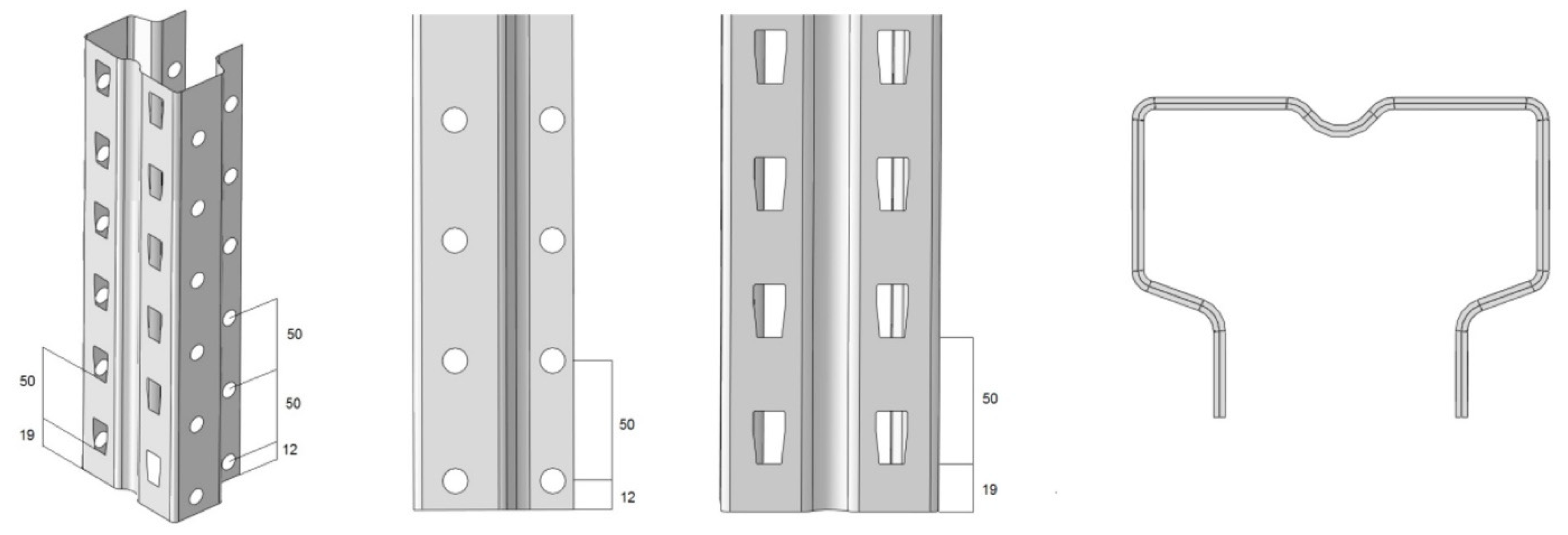
Applsci 11 11056 g001aApplsci 11 11056 g001b
Figure 2. Upright configuration details (dimensions are in millimeters).
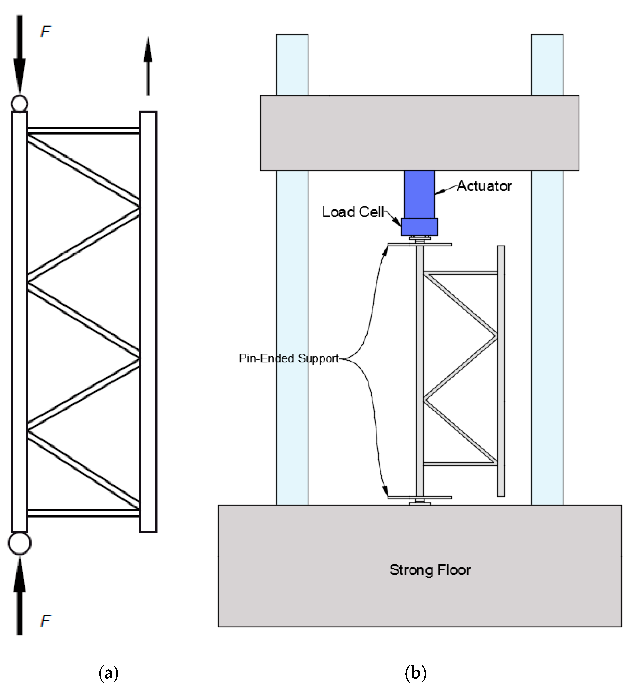
Applsci 11 11056 g002
Figure 3. (a) Schematic of compressive test on uprights; (b) testing rig.
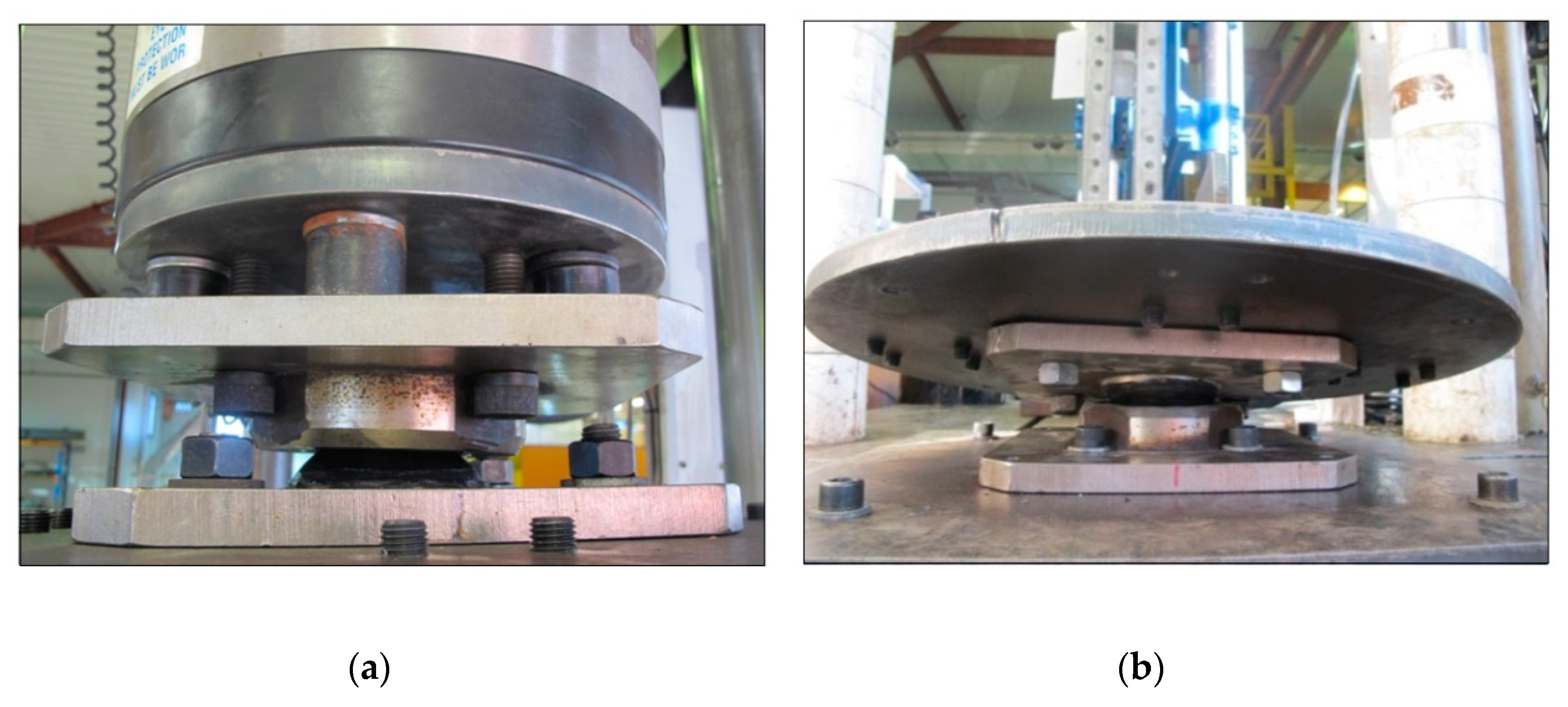
Applsci 11 11056 g003
Figure 4. (a) Ball bearing; (b) cap plates.
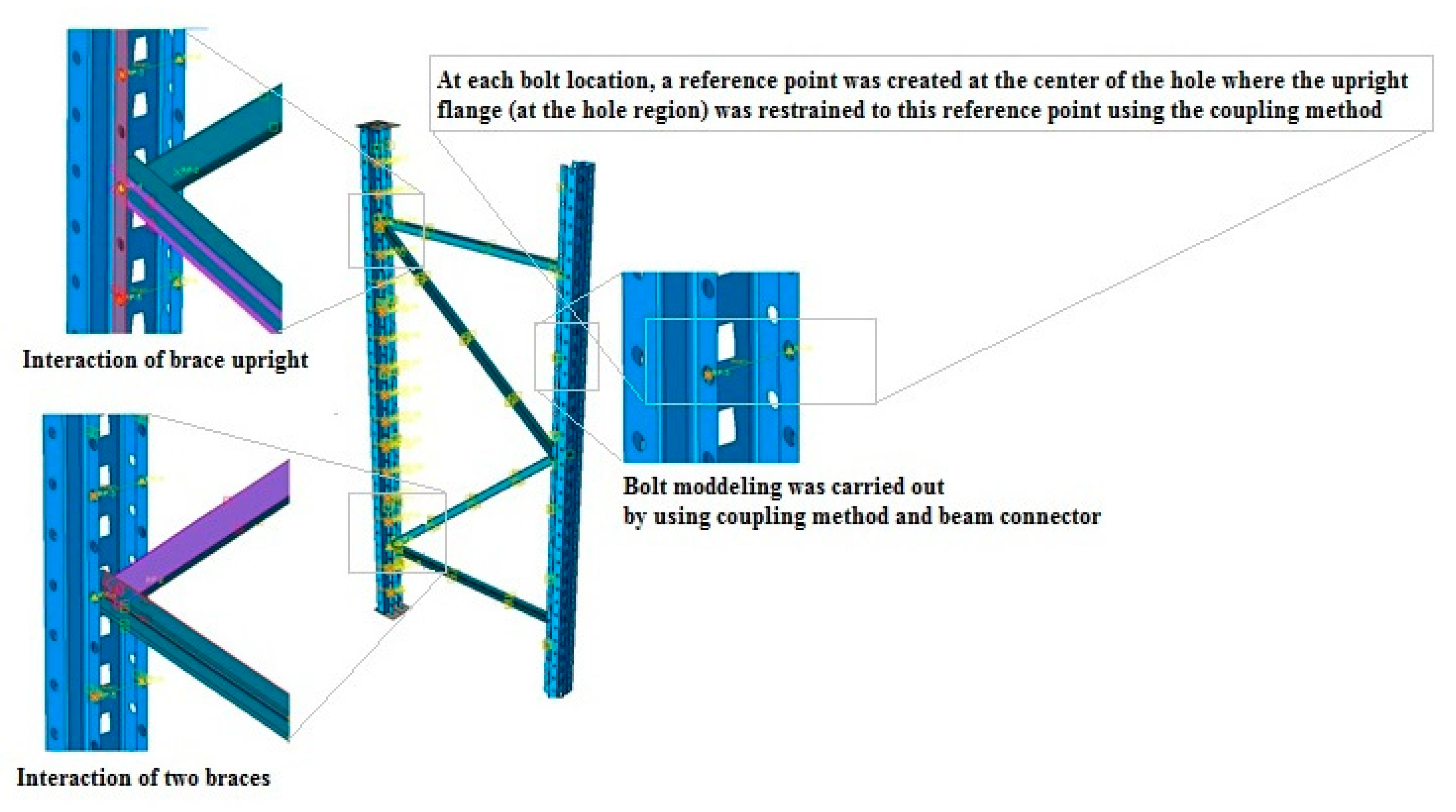
Applsci 11 11056 g004
Figure 5. Interaction and connection properties of a typical model.
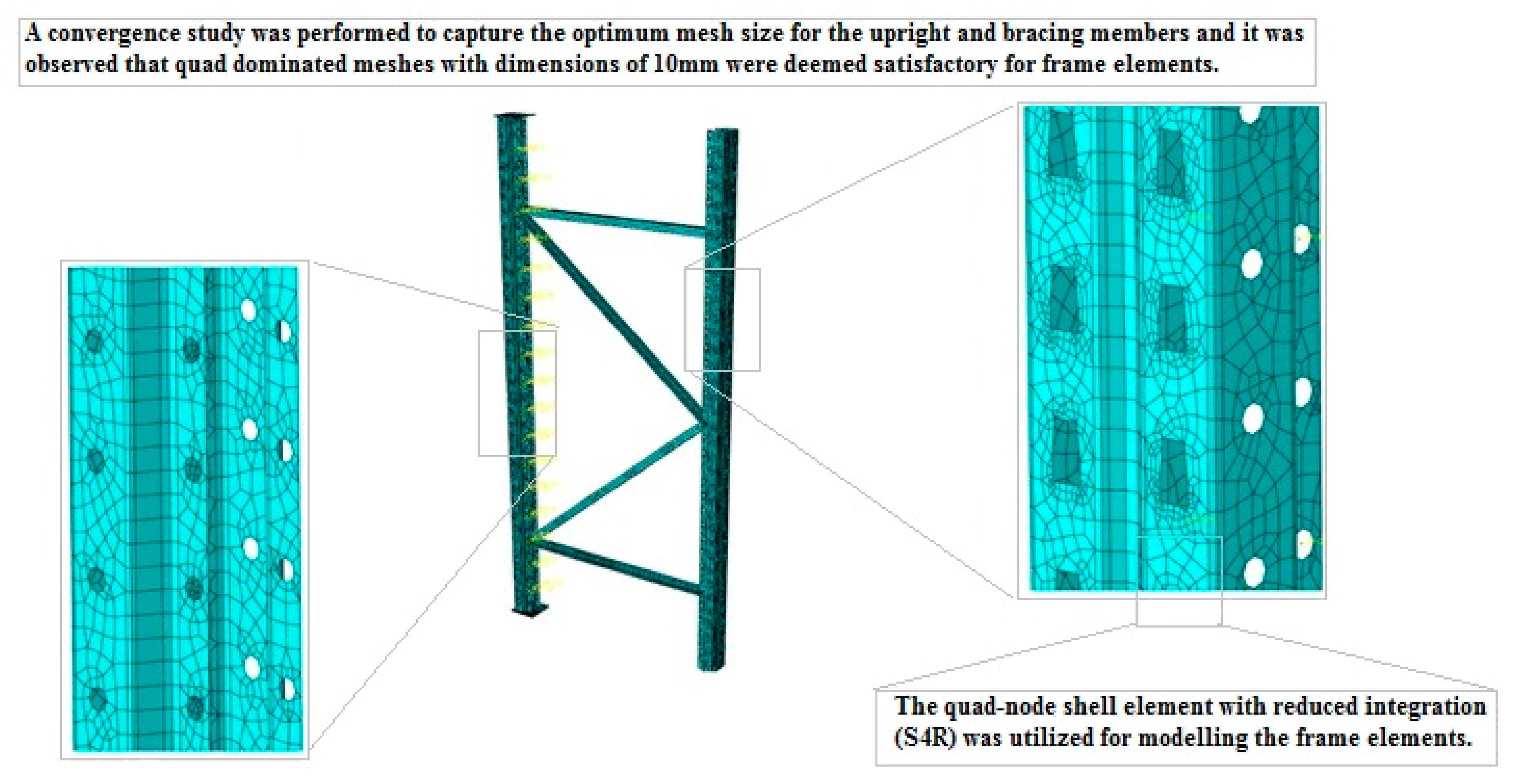
Applsci 11 11056 g005
Figure 6. A typical model with a mesh matrix view on the polygon and circular perforations.
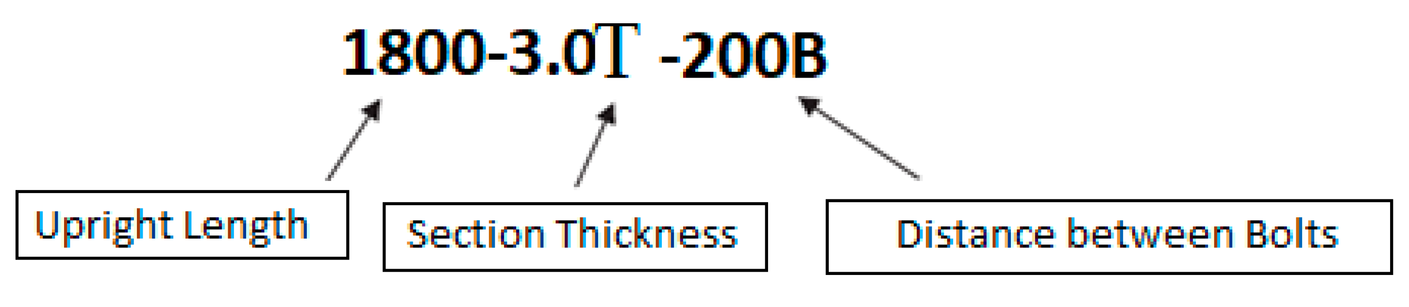
Applsci 11 11056 g006
Figure 7. Designation of models.
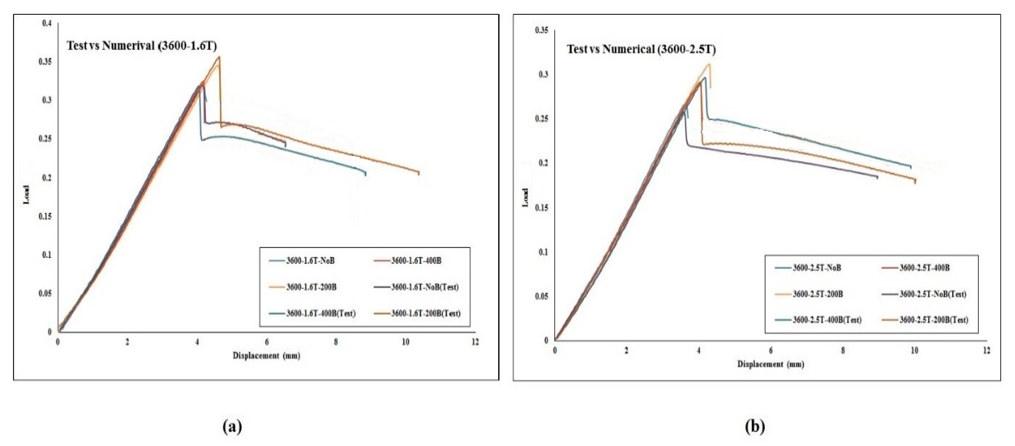
Applsci 11 11056 g007
Figure 8. Comparison of the experimental and numerical results of normalised load for (a) 3600L-1.6T, (b)3600L-2.5T.
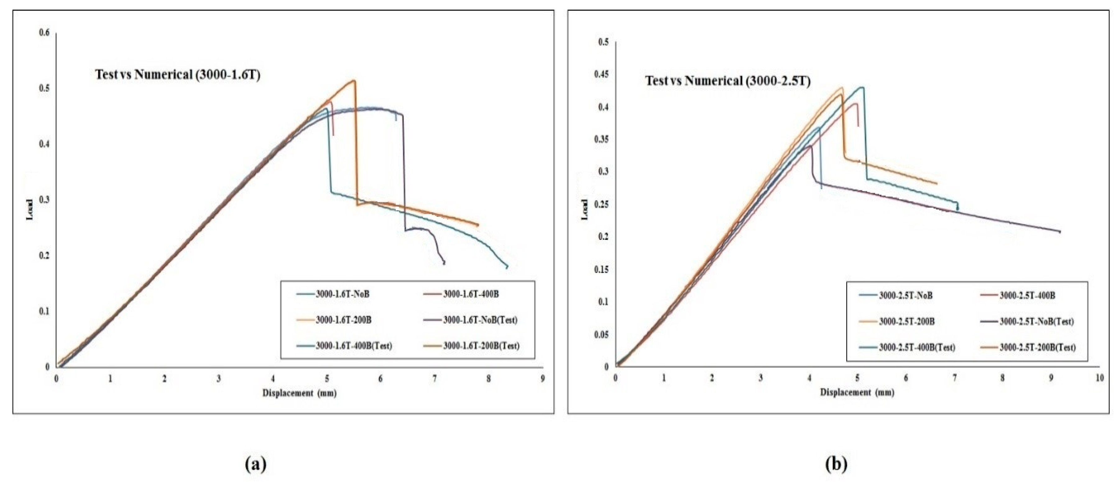
Applsci 11 11056 g008
Figure 9. Comparison of experimental and numerical results of normalised load for (a) 3000L-1.6T, (b) 3000L-2.5T.
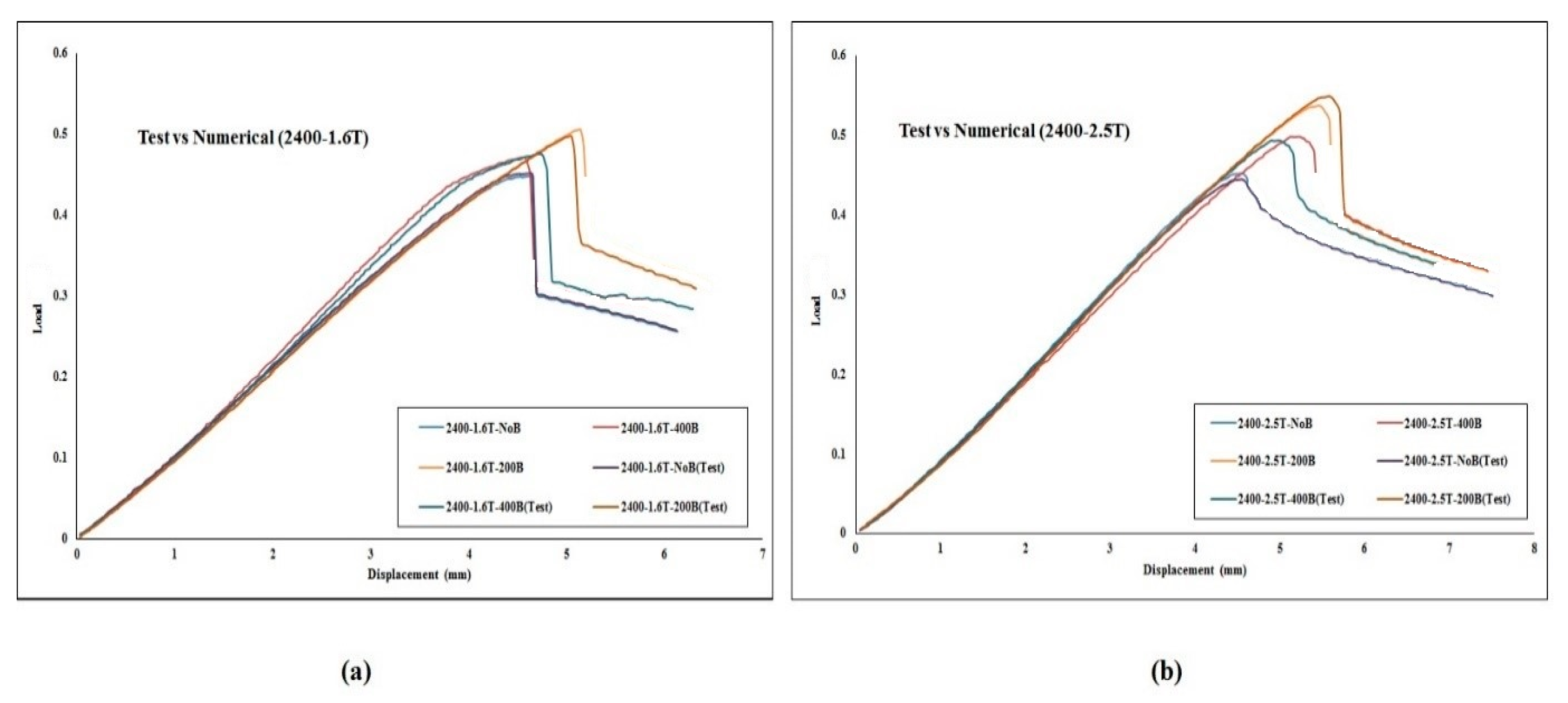
Applsci 11 11056 g009
Figure 10. Comparison of experimental and numerical results of normalised load for (a) 2400L-1.6T, (b) 2400L-2.5T.
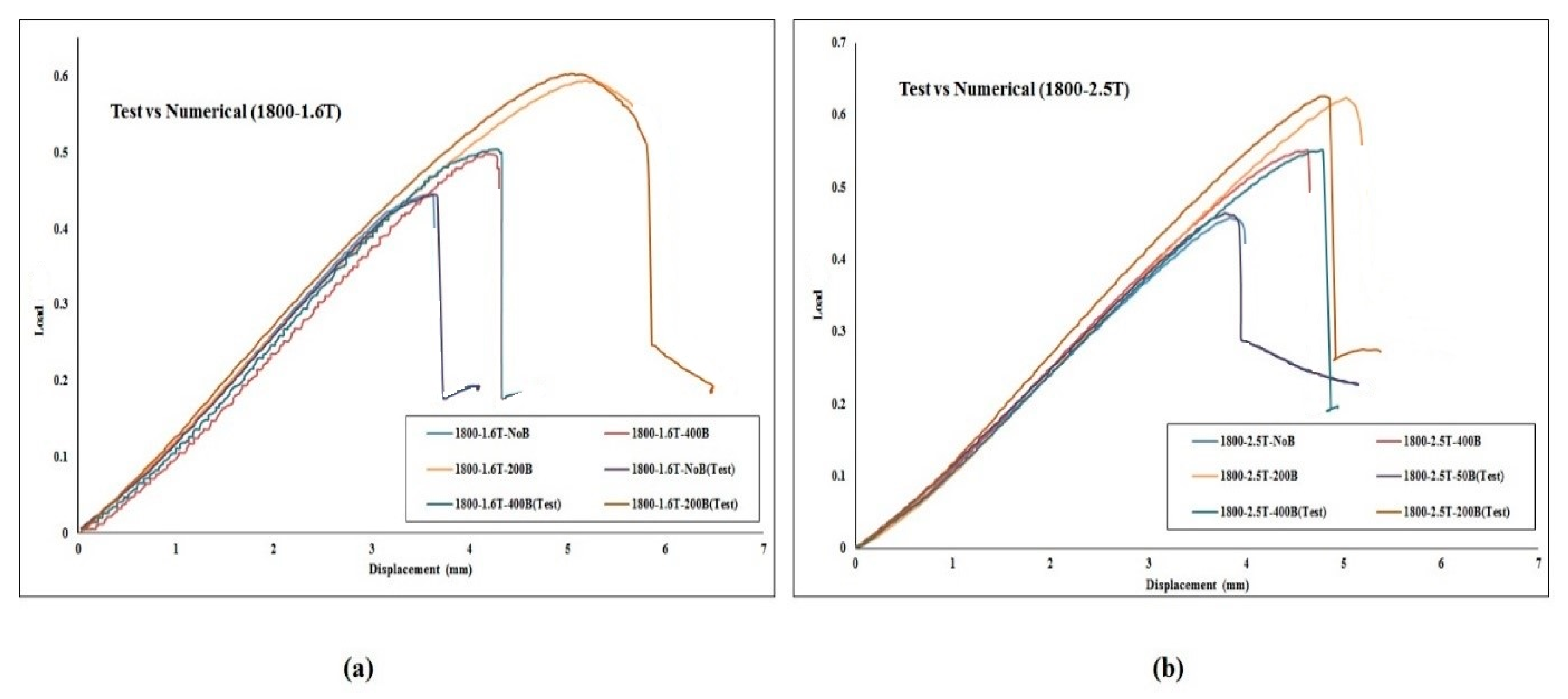
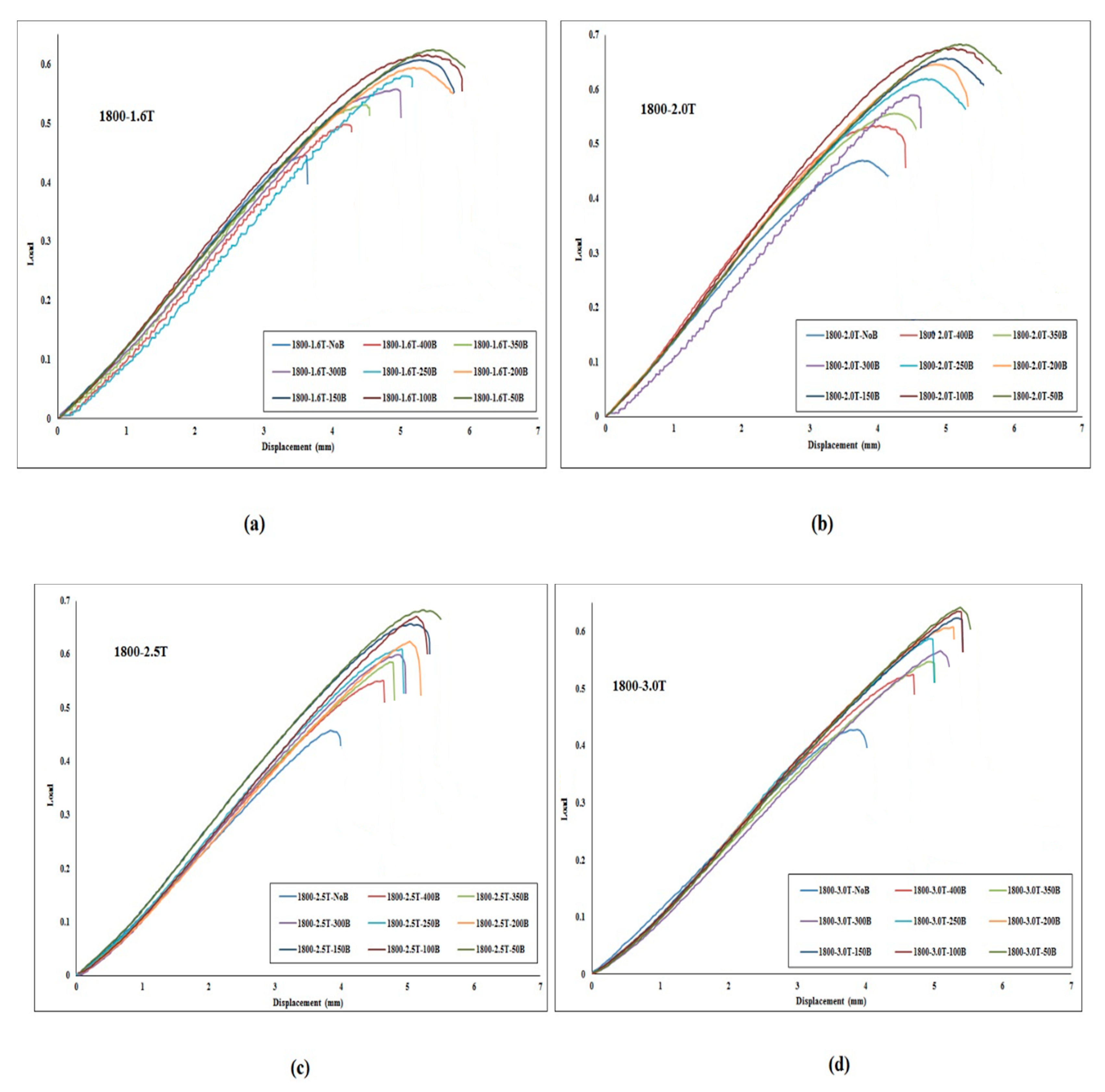
Applsci 11 11056 g010
Figure 11. Comparison of experimental and numerical results of normalised load for (a) 1800L-1.6T, (b) 1800L-2.5T.
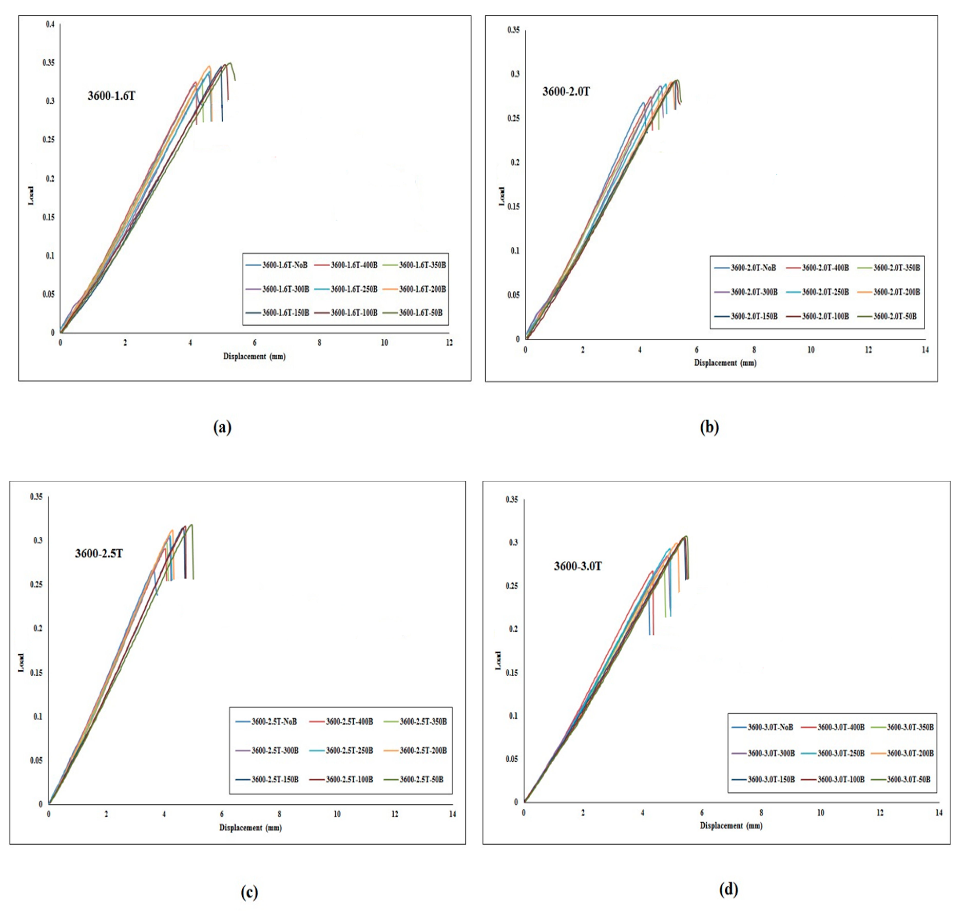
Applsci 11 11056 g011
Figure 12. Normalised load-displacement diagrams of the FE results for: (a) 3600L-1.6T, (b) 3600L-2.0T, (c) 3600L-2.5T, and (d) 3600L-3.0T models.
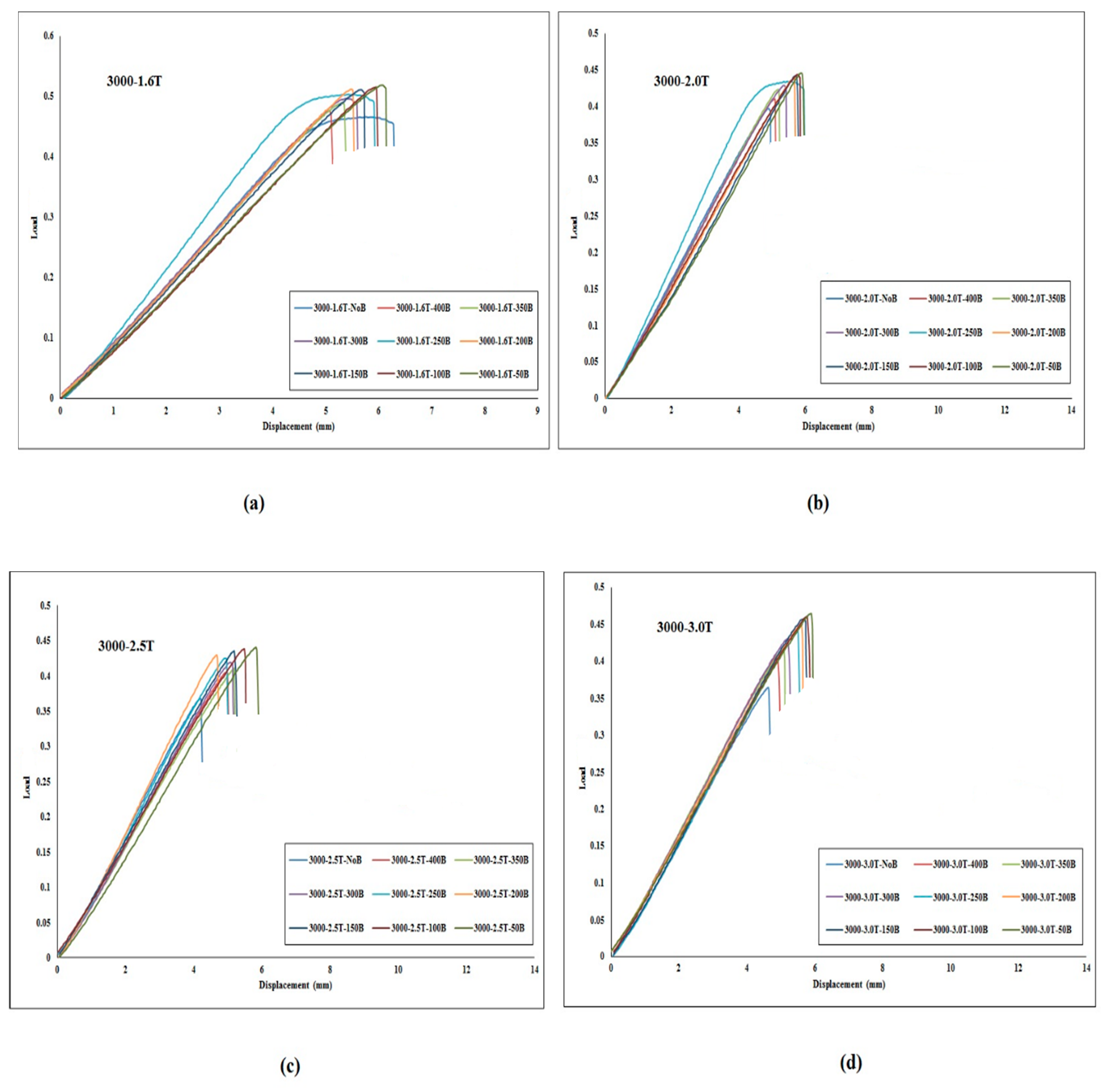
Applsci 11 11056 g012
Figure 13. Normalised load-displacement diagrams of the FE results for: (a) 3000L-1.6T, (b) 3000L-2.0T, (c) 3000L-2.5T, and (d) 3000L-3.0T models.
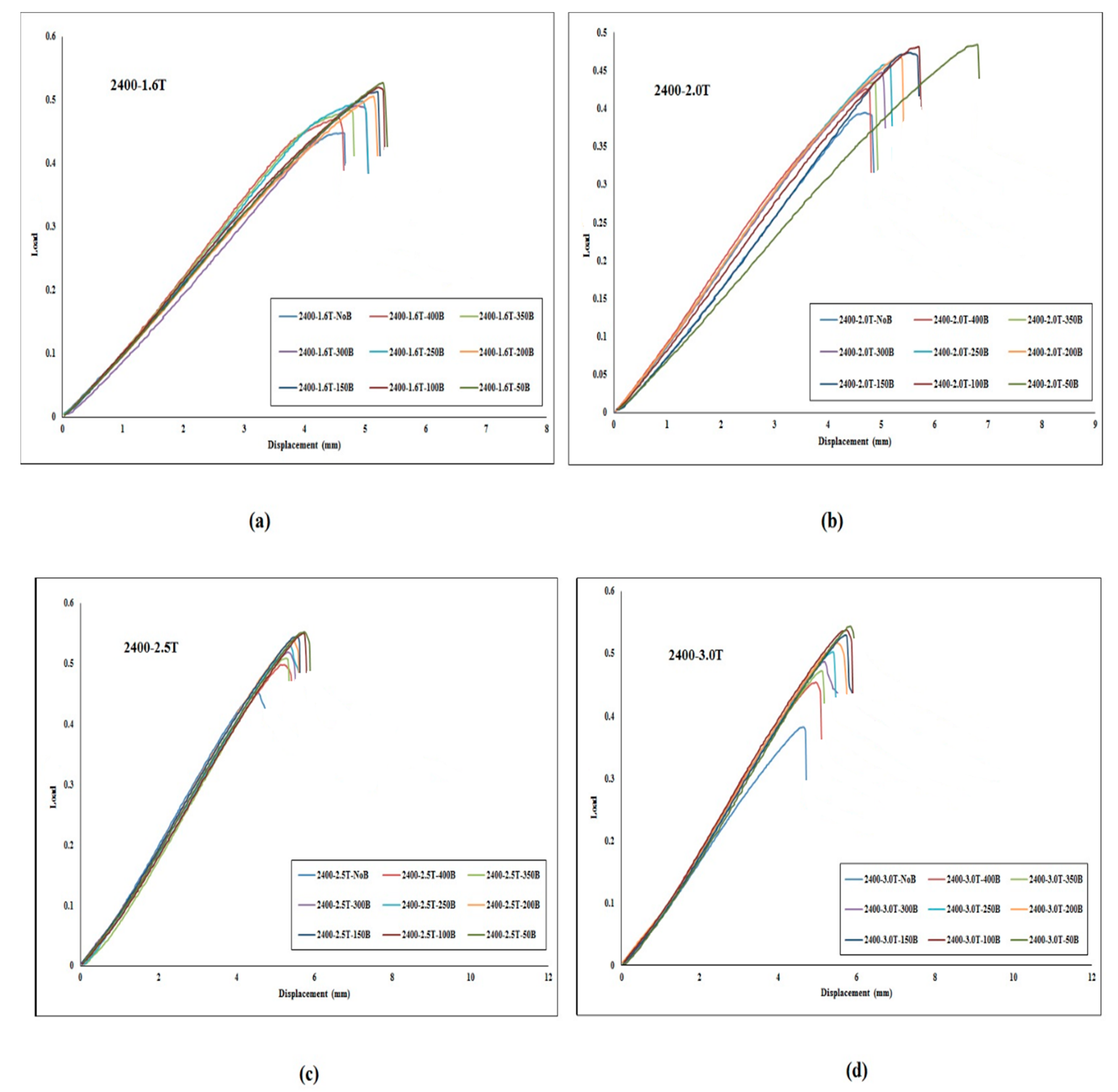
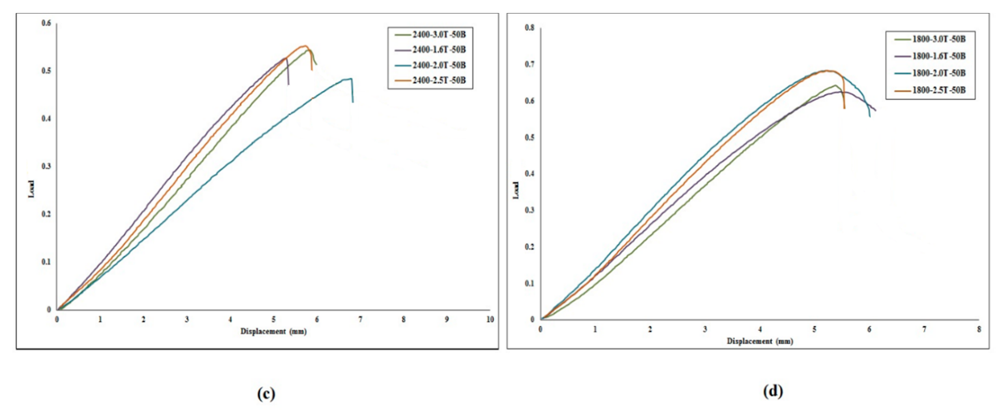
Applsci 11 11056 g013
Figure 14. Normalised load-displacement diagrams of the FE results for: (a) 2400L-1.6T, (b) 2400L-2.0T, (c) 2400L-2.5T, and (d) 2400L-3.0T models.
Applsci 11 11056 g014
Figure 15. Normalised load-displacement diagrams of the FE results for: (a) 1800L-1.6T, (b) 1800L-2.0T, (c) 1800L-2.5T, and (d) 1800L-3.0T models.
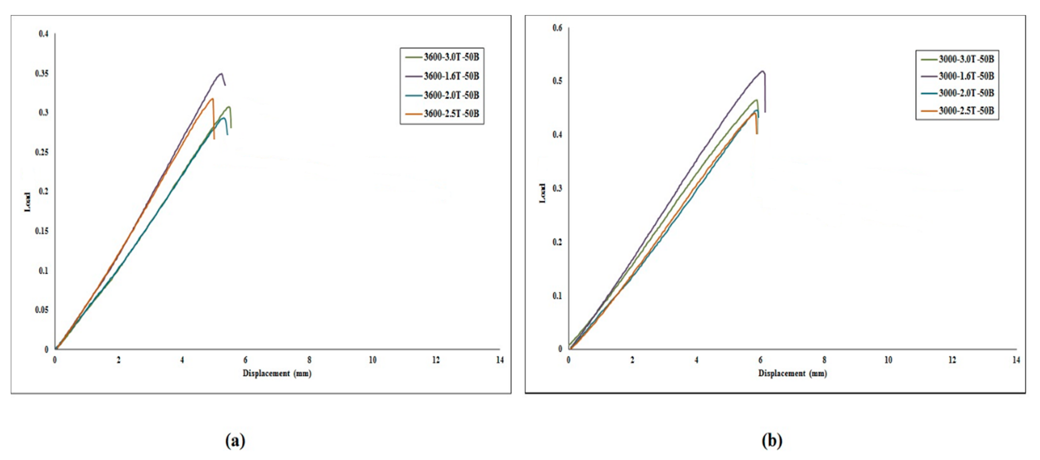
Applsci 11 11056 g015
Figure 16. Normalised load-displacement diagrams of the FE results for: (a) 3600L-50B, (b) 3000L-50B, (c) 2400L-50B, and (d) 1800L-50B models.
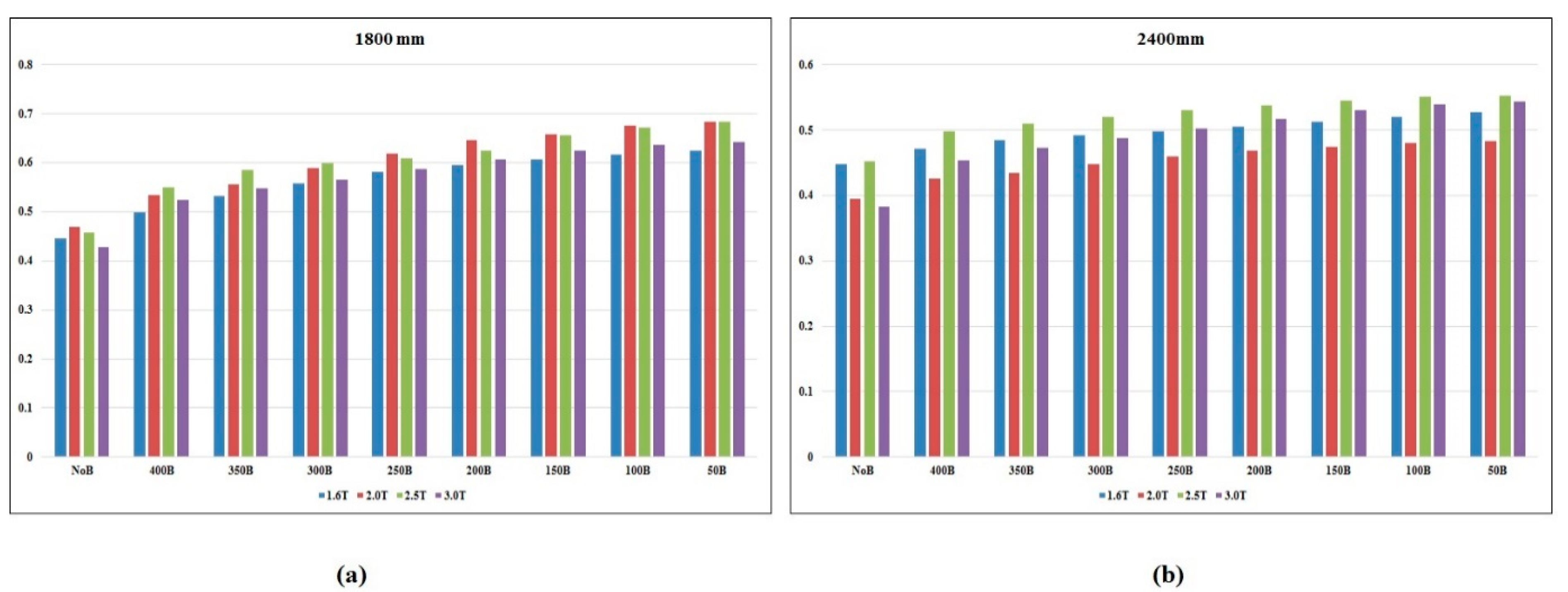
Applsci 11 11056 g016aApplsci 11 11056 g016b
Figure 17. Ultimate load capacities based on thickness and reinforcement spacing for (a) 1800 mm models and (b) 2400 mm models.
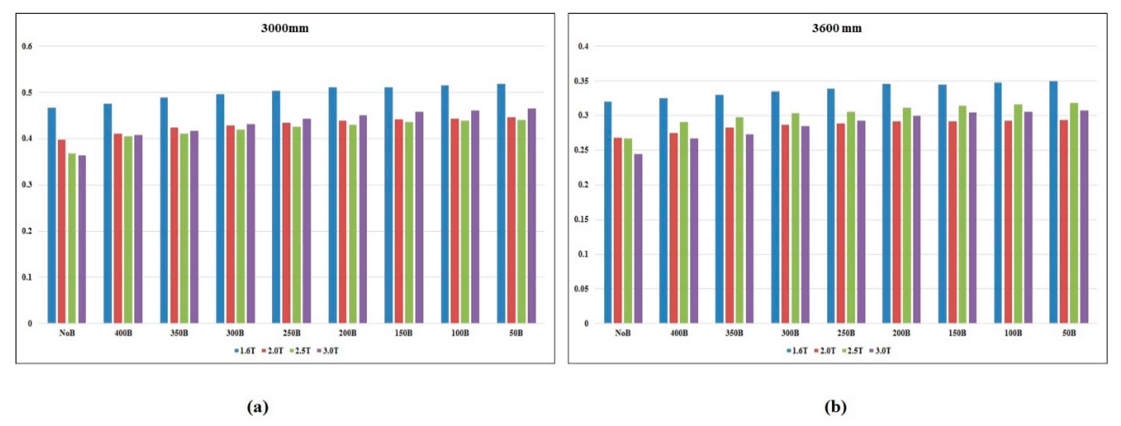
Applsci 11 11056 g017
Figure 18. Ultimate load capacities based on thickness and reinforcement spacing for (a) 3000 mm models and (b) 3600 mm models.
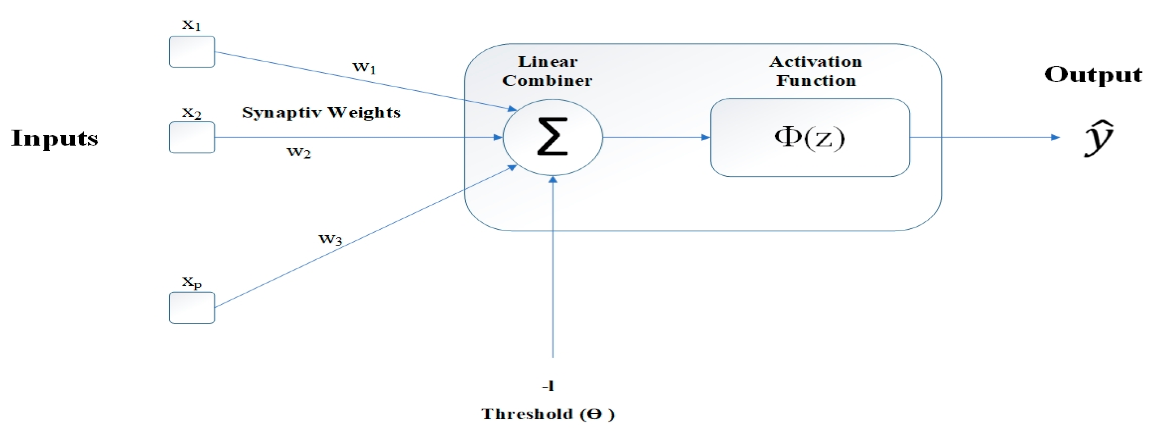
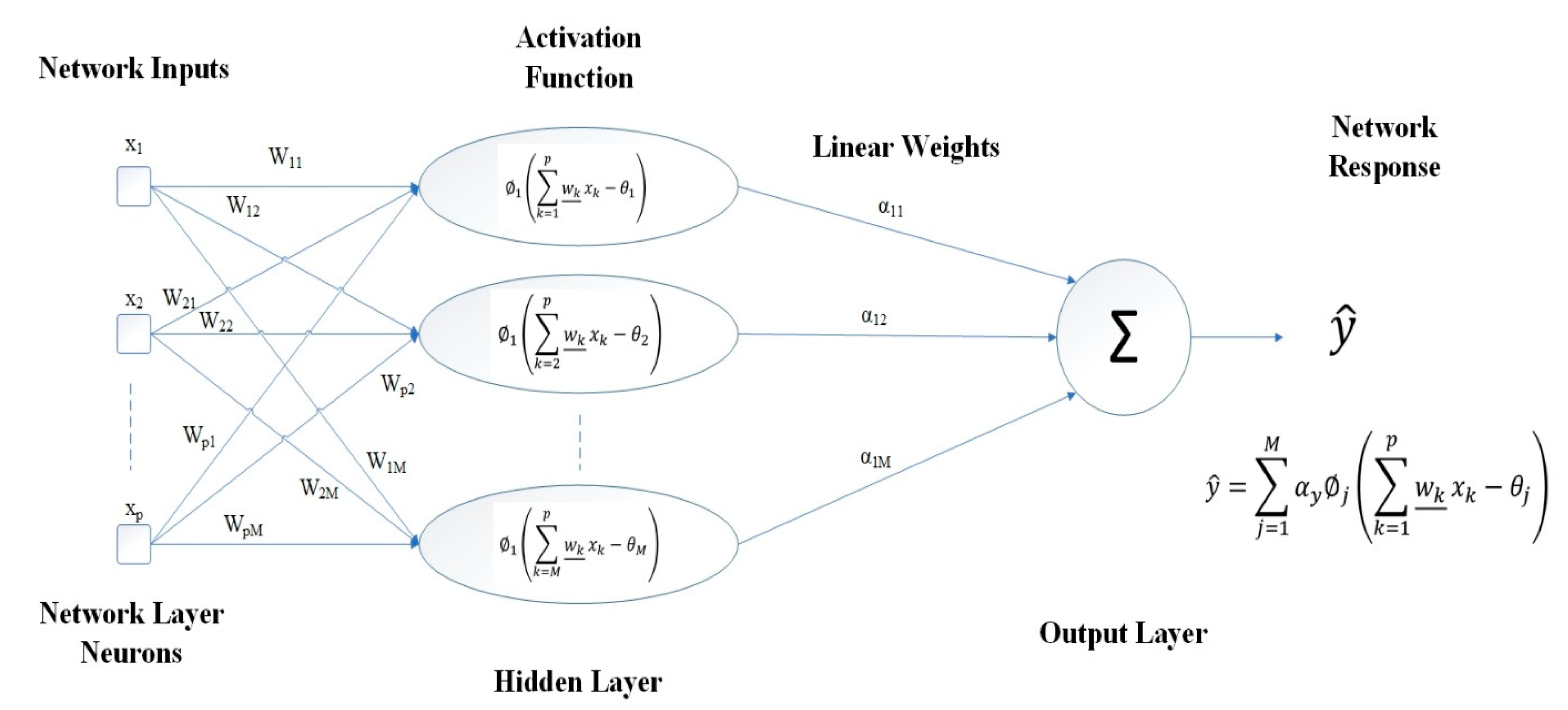
Applsci 11 11056 g018
Figure 19. Schematic representation of MLP neuron.
Applsci 11 11056 g019
Figure 20. Flowchart of typical single line hidden layer MLP for identifying a problem.
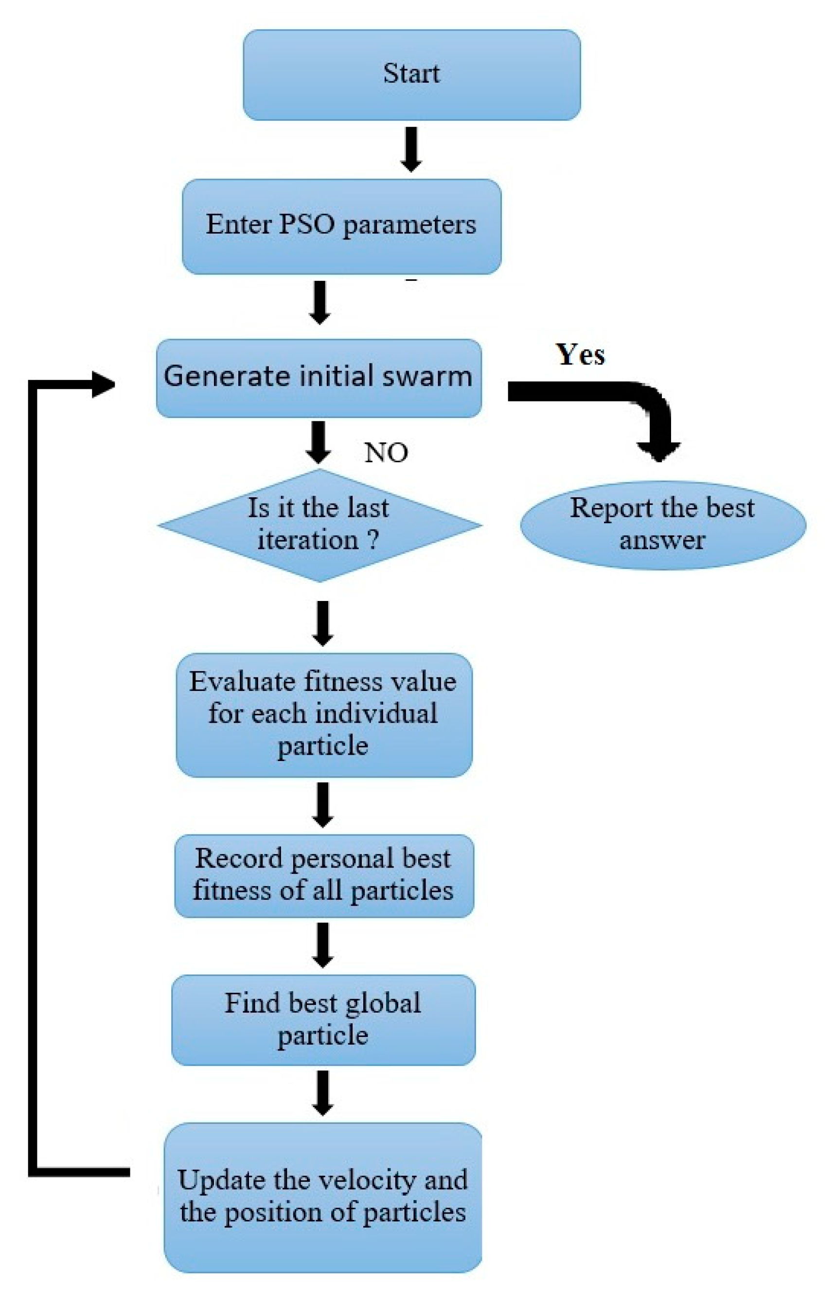
Applsci 11 11056 g020
Figure 21. PSO sequential flowchart.
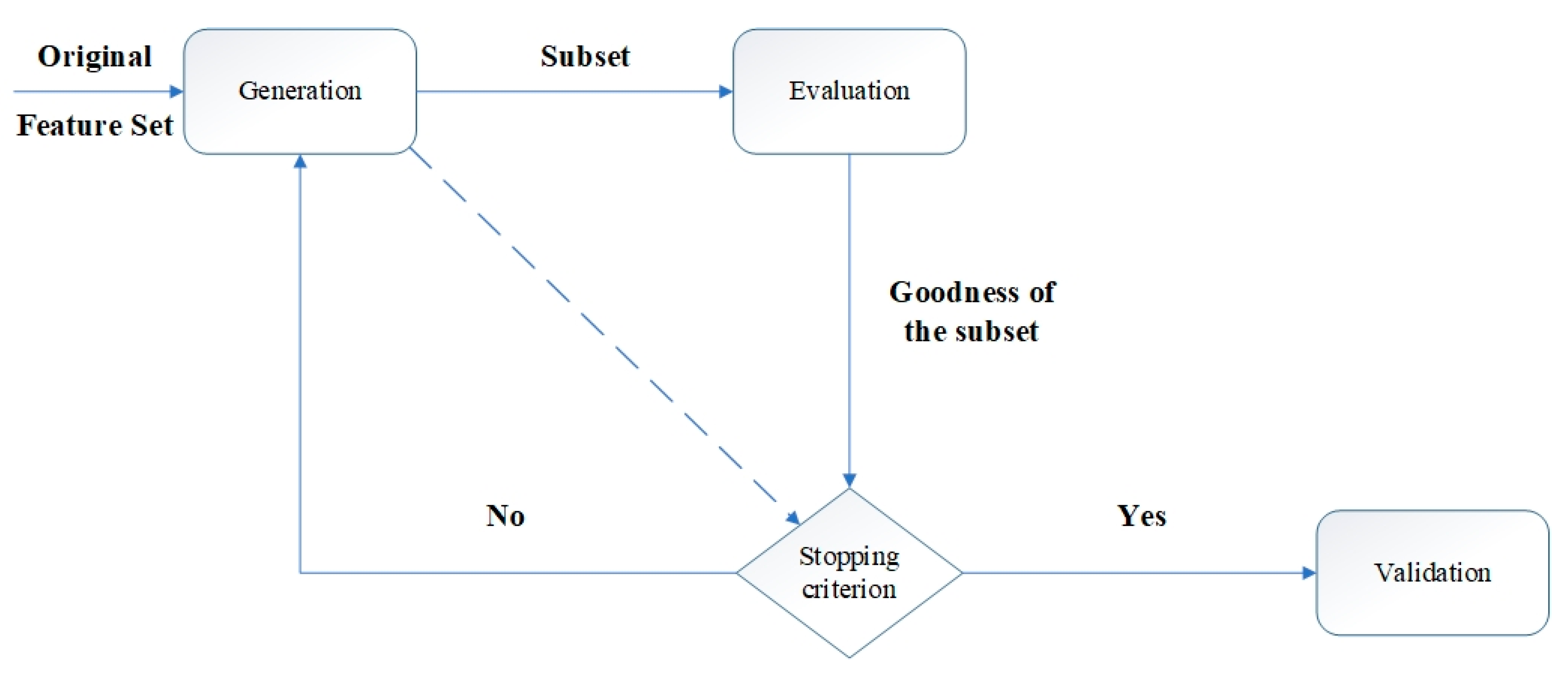
Applsci 11 11056 g021
Figure 22. Feature selection technique steps.
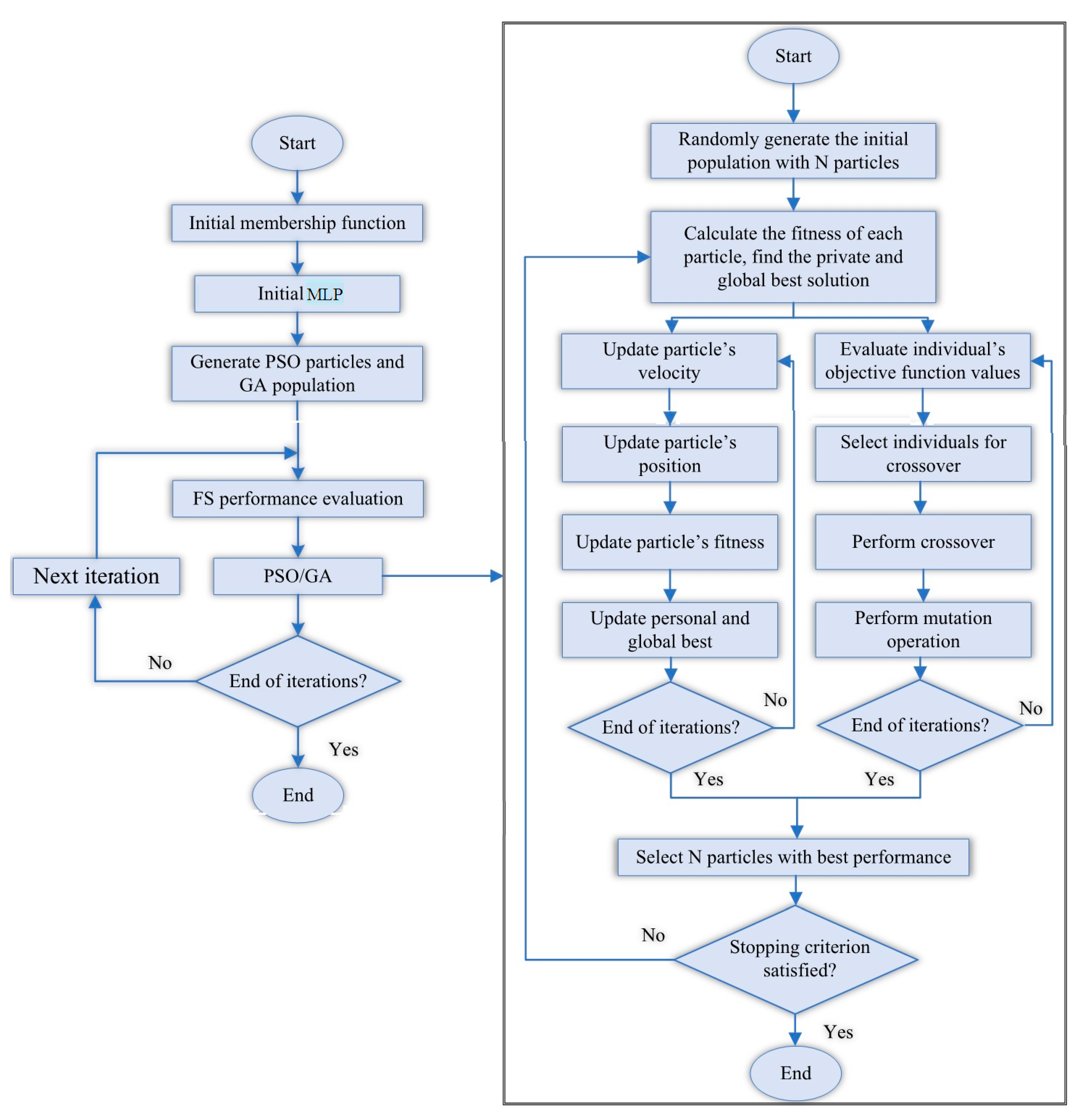
Applsci 11 11056 g022
Figure 23. The flowchart of the sequential combination of hybrid MLP-PSO-FS algorithm.
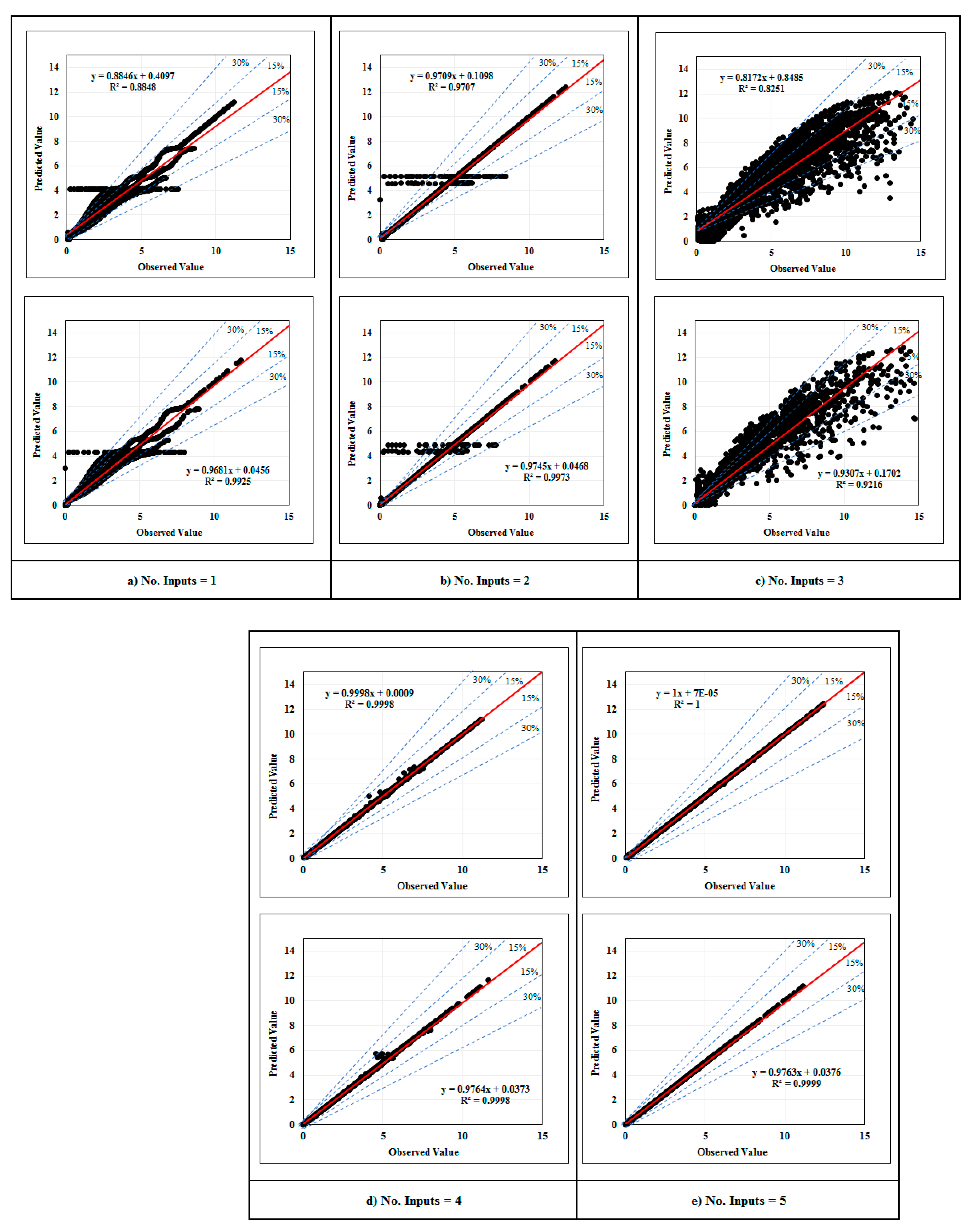
Applsci 11 11056 g023
Figure 24. Regression of the training (above charts) and testing (below charts) phase results with measured values of displacement for (a) one input, (b) two inputs, (c) three inputs, (d) four inputs, (e) five inputs.
Applsci 11 11056 g024
Figure 25. Tolerance diagram of the displacement prediction corresponding to the MPF model with five inputs: (above) training phase, and (below) testing phase.
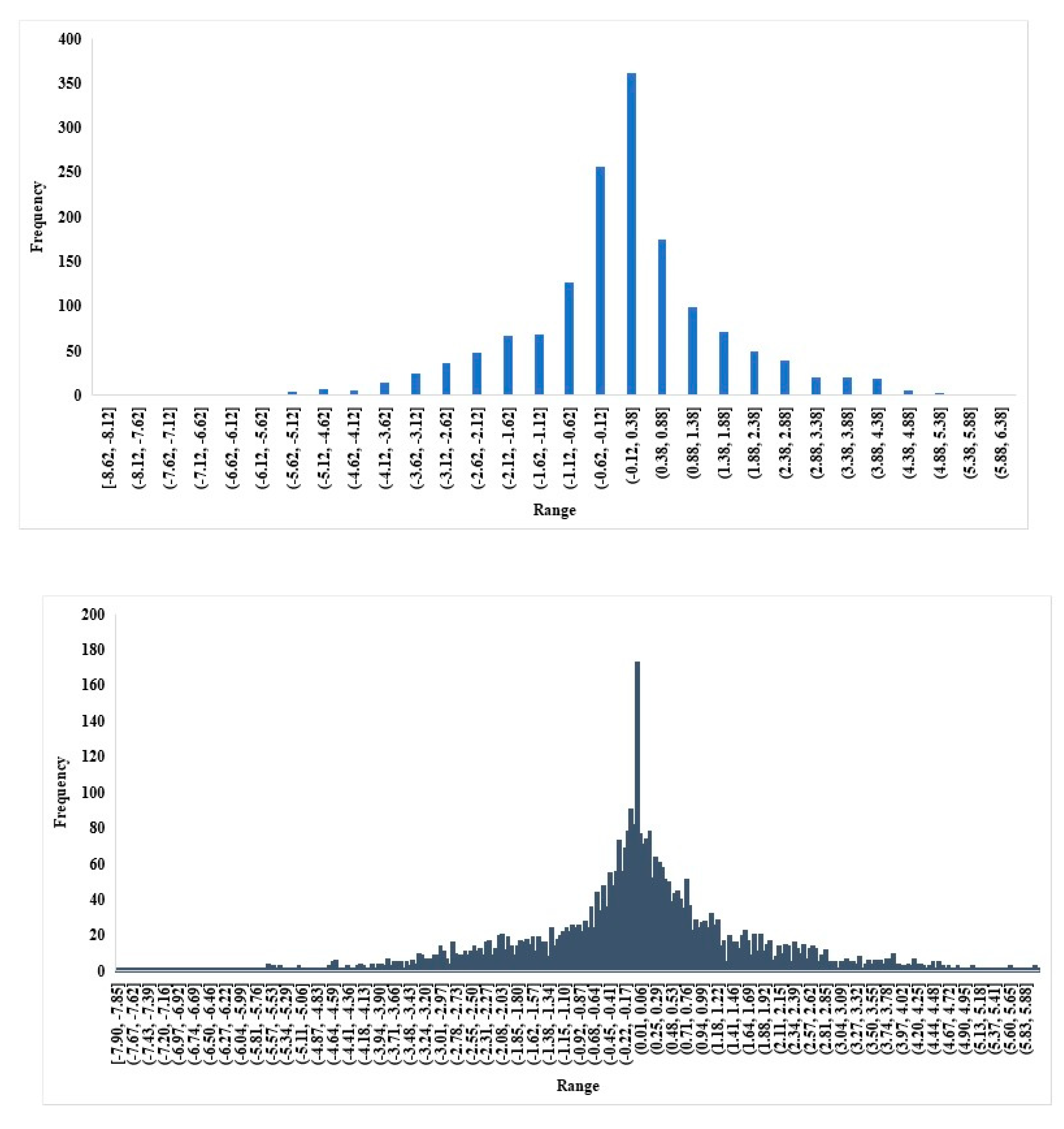
Applsci 11 11056 g025
Figure 26. Error histograms for displacement prediction by the MPF model with five inputs: (above) training phase, and (below) testing phase.
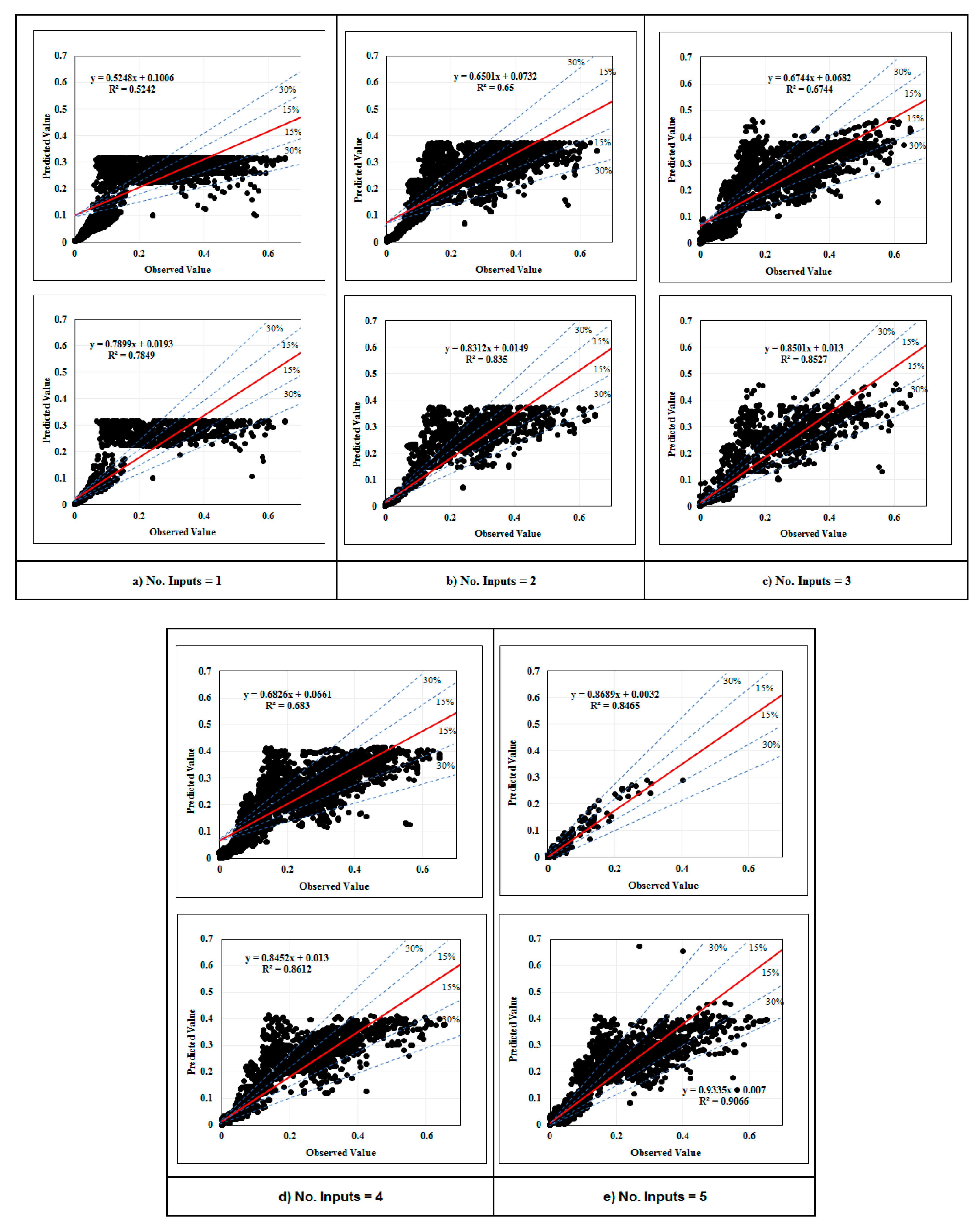
Applsci 11 11056 g026
Figure 27. Regression of the training (above charts) and testing (below charts) phase results with measured values of normalised load for (a) one input, (b) two inputs, (c) three inputs, (d) four inputs, (e) five inputs.
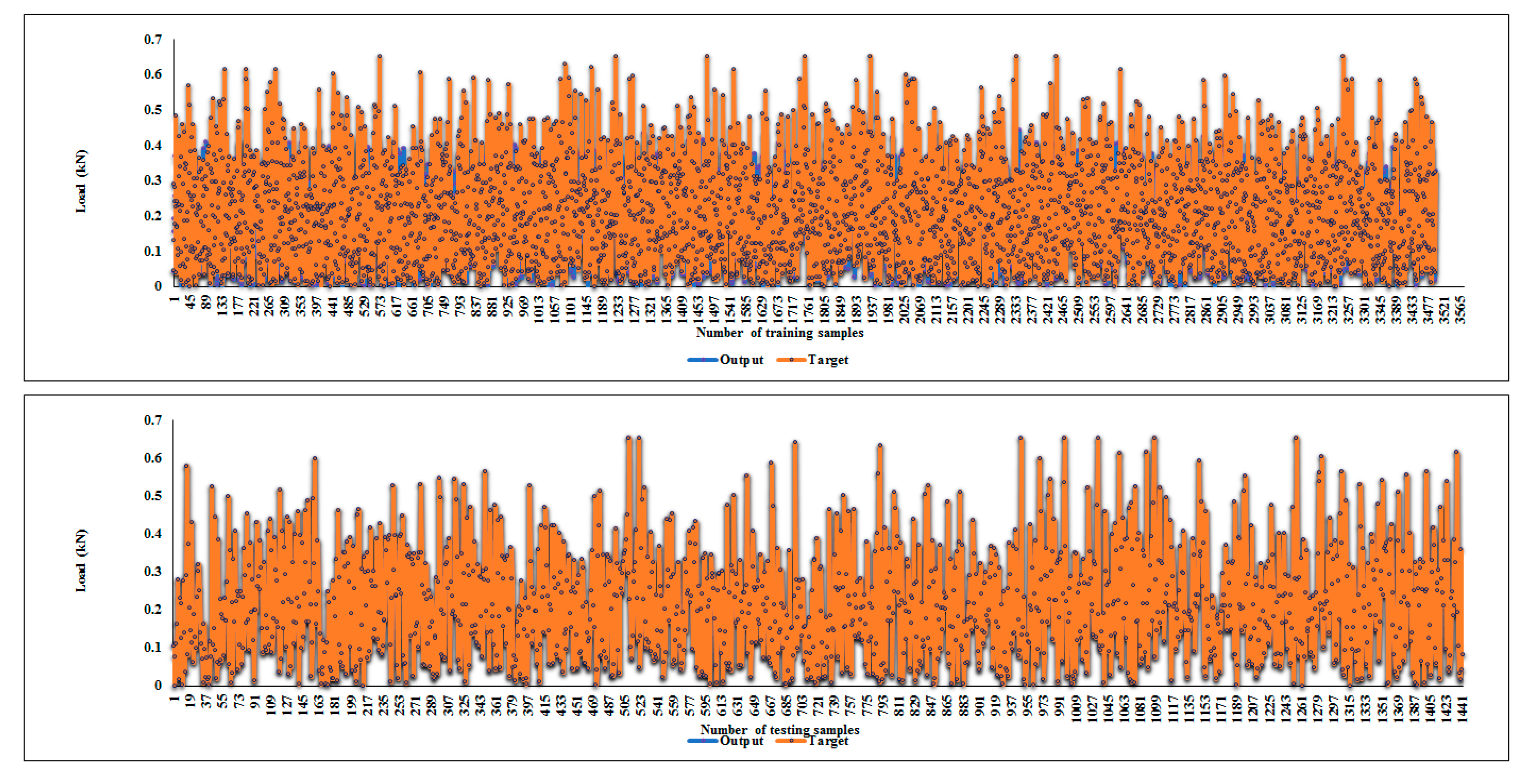
Applsci 11 11056 g027
Figure 28. The MPF (five inputs) prediction vs experimental diagram for ultimate load: (above) training phase, (below) testing phase.
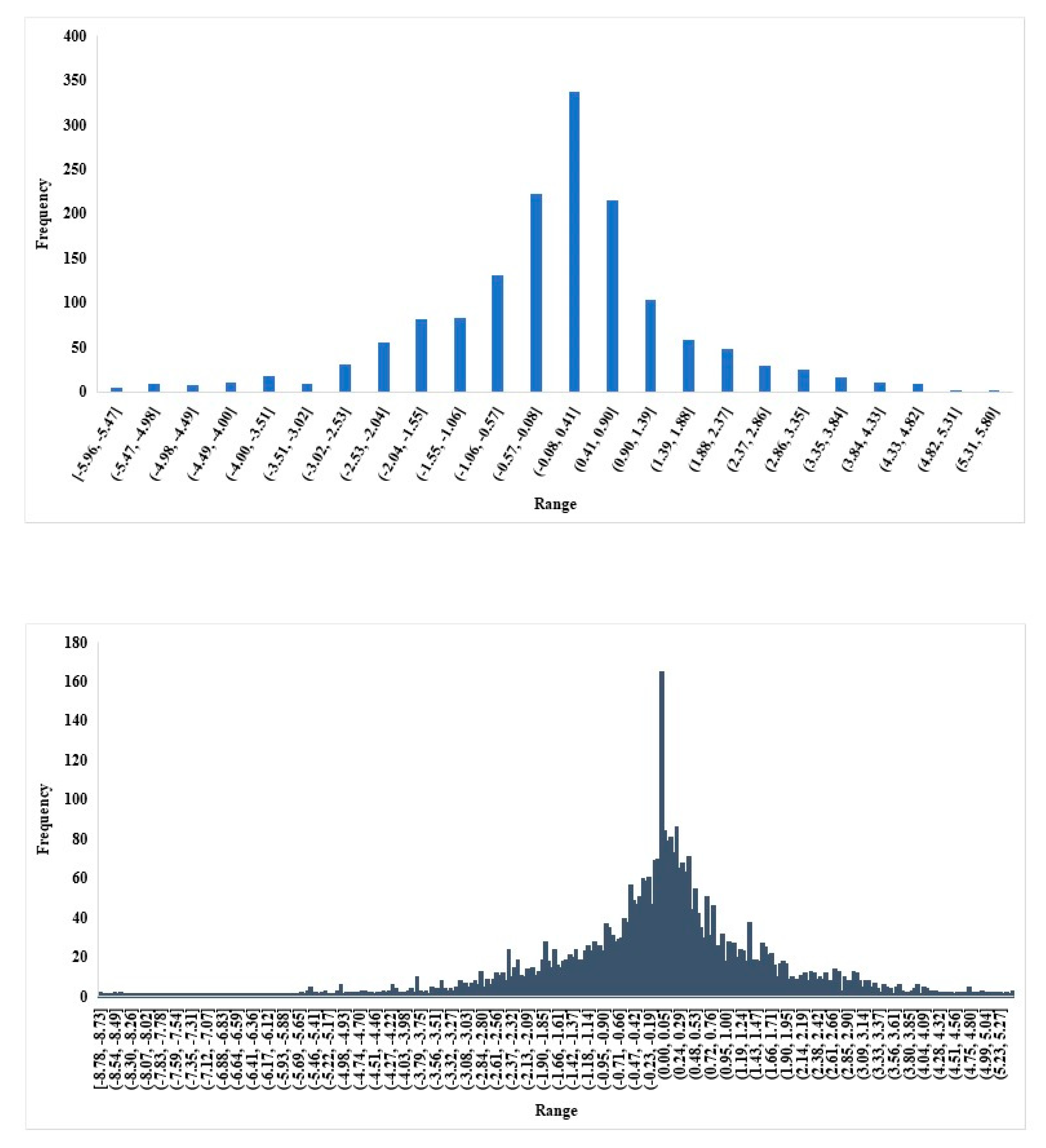
Applsci 11 11056 g028
Figure 29. The MPF (five inputs) error histograms for ultimate load prediction: (above) training phase and (bellow) testing phase.
Applsci 11 11056 g029
Table 1. Ultimate normalised compressive capacities for 3600 mm models based on reinforcement spacing.
3600 mmNoB400B350B300B250B200B150B100B50B
1.6T0.3203550.3249570.3296940.3343110.3384520.3455720.3450140.347480.349518
2.0T0.2678650.2745810.2832070.2866140.2888060.2911520.2918670.2927150.293467
2.5T0.2666150.2907980.297350.3028960.305180.3116460.3140020.3158190.317829
3.0T0.2440690.2667560.2733360.2846060.2926420.2991020.3040170.3057070.30739
Table 2. Ultimate normalised compressive capacities for 3000 mm models based on reinforcement spacing.
3000 mmNoB400B350B300B250B200B150B100B50B
1.6T0.4661920.4761690.4889060.4964210.5035790.511750.5110990.5149370.518591
2.0T0.3972640.4102940.4234950.4290790.434540.4383750.4419860.4439070.445772
2.5T0.3679050.4046570.4112690.4193280.424850.4299130.4355150.4382430.440754
3.0T0.3642670.4078490.4166350.4313770.4425950.4500410.4576850.4614080.464957
Table 3. Ultimate normalised compressive capacities for 2400 mm models based on reinforcement spacing.
2400 mmNoB400B350B300B250B200B150B100B50B
1.6T0.448090.471590.4840620.4911350.4983480.5057940.5126340.5201270.527014
2.0T0.3945460.4260410.4346780.447410.4588770.4689280.4735450.4807740.483447
2.5T0.4521610.4980860.5088370.5192910.5295060.5374280.5450830.5500860.552796
3.0T0.3824840.4540620.4720060.487010.5025580.5169780.5295110.5382970.543857
Table 4. Ultimate normalised compressive capacities for 1800 mm models based on reinforcement spacing.
1800 mmNoB400B350B300B250B200B150B100B50B
1.6T0.4461350.4981620.5312490.5577740.5802850.5942110.6071480.6157570.624738
2.0T0.4695980.5332960.5557080.5895110.6194430.6457630.6570060.675620.682954
2.5T0.4578490.5499370.5854680.5995850.6083110.6241560.6567140.6710630.682757
3.0T0.4284730.5237040.5472870.5662930.5877120.6068220.62350.6355130.642487
Table 5. Best achieved results for displacement estimation.
Phase Network Result
R2RNSRMSEMAEWI
Test0.9991.0001.0000.0010.0001.000
Train1.0001.0001.0000.0000.0001.000
Table 6. Best obtained results for normalised load estimation.
PhaseNetwork Result
R2RNSRMSEMAEWI
Test0.9070.8000.4351.6781.2030.882
Train0.8470.8200.5111.5901.1370.895
Table 7. Parameter characteristics used for PSO in this study.
FIS ClustersPopulation SizeIterationsInertia WeightDamping RatioLearning Coefficient
PersonalGlobal
10150~35045~10010.9823
Table 8. Parameter characteristics used for MLP and FE.
Parameter characteristics used for the MLP
Hidden LayersTraining Function
10Levenberg–Marquardt back-propagation (LMBP)
Parameter characteristics used for FS
Number of runsNumber of functions(nf)
31~5
Table 9. Selected input composition for displacement prediction based on feature-selection method *.
FeatureNumber of Inputs
12345
Length XX
Bolt XXX
Thickness XXXX
Shape   factor   ( Ag   × σ y ) X
Axial loadXXXXX
*: marks represents the composition of the input in each model.
Table 10. Calculated accuracy criteria for the performance of the implemented models to displacement prediction (iteration = 45).
Train
The MPF Network
IterationPopulationnfR2rNSRMSEMAEWI
4525010.8850.9410.8700.0350.0260.969
4525020.9710.9850.9700.0180.0030.993
4525030.8250.9960.9927.2445.2700.998
4525040.9991.0001.0000.0010.0001.000
452505 *1.0001.0001.0000.0000.0001.000
Test
The MPF Network
IterationPopulationnfR2rNSRMSEMAEWI
4525010.9920.9350.8540.0380.0280.965
4525020.9970.9780.9550.0220.0040.989
4525030.9210.9070.7987.1995.2460.951
4525040.9991.0001.0000.0010.0001.000
452505 *0.9991.0001.0000.0010.0001.000
* Most precise predicted value in comparison to the measured value.
Table 11. Selected features as input for ultimate load prediction *.
FeatureNumber of Inputs
12345
LengthX XX
Bolt XXXX
Thickness XXX
Shape   factor   ( Ag   × σ y ) XX
Displacement XX X
*: marks represents the composition of the input in each model.
Table 12. Calculated accuracy criteria of the MPF model for the performance of the implemented models to ultimate load prediction (iteration = 45).
Train
The MPF Network
IterationPopulationnfR2rNSRMSEMAEWI
15025010.5240.7090.0111.9661.3860.816
15025020.6500.7960.4221.6721.1210.879
15025030.6740.8120.4841.6201.1480.890
15025040.6830.8180.5031.5751.1250.894
1502505 *0.8470.8200.5111.5901.1370.895
Test
The MPF Network
IterationPopulationnfR2rNSRMSEMAEWI
15025010.7850.697−0.0341.9841.4000.809
15025020.8350.7820.3571.7621.1890.869
15025030.8530.8060.4641.6551.1590.886
15025040.8120.8220.4891.6391.1630.894
1502505 *0.9070.8000.4351.6781.2030.882
* The most precise predicted value in comparison to the measured value.
Publisher’s Note: MDPI stays neutral with regard to jurisdictional claims in published maps and institutional affiliations.

