Design and Control of an Omnidirectional Mobile Wall-Climbing Robot

Abstract

Omnidirectional mobile wall-climbing robots have better motion performance than traditional wall-climbing robots. However, there are still challenges in designing and controlling omnidirectional mobile wall-climbing robots, which can attach to non-ferromagnetic surfaces. In this paper, we design a novel wall-climbing robot, establish the robot’s dynamics model, and propose a nonlinear model predictive control (NMPC)-based trajectory tracking control algorithm. Compared against state-of-the-art, the contribution is threefold: First, the combination of three-wheeled omnidirectional locomotion and non-contact negative pressure air chamber adhesion achieves omnidirectional locomotion on non-ferromagnetic vertical surfaces. Second, the critical slip state has been employed as an acceleration constraint condition, which could improve the maximum linear acceleration and the angular acceleration by $164.71\%$ and $22.07\%$ on average, respectively. Last, an NMPC-based trajectory tracking control algorithm is proposed. According to the simulation experiment results, the tracking accuracy is higher than the traditional PID controller.

1. Introduction

The wall-climbing robot mainly consists of two modules: the locomotion module and the adhesion module. For the locomotion types, arms and legs [1] are good at overcoming obstacles but have drawbacks in velocity, wheels and chains [2] have advantages in continuous and fast movement but cannot handle large obstacles, sliding frames [3] are simple in both structure and control but move slowly compared with wheels and chains, and wires and rails [4] are safe and carry a considerable payload weight but demand external guidance and equipment. For the adhesion types, magnetic adhesion [5] has a strong adhesion force but demands a ferromagnetic wall, passive suction cups [6] have lower energy consumption, while active suction chambers [7,8,9] have stable adhesion, mechanical adhesion [10,11,12] has low energy consumption and is stable but usually requires unique construction or materials on the wall surface, and chemical adhesion [13] has low energy consumption when the robot is not moving but is highly influenced by wall material.

According to the literature [14,15], there are few wall-climbing robotic systems attached to non-ferromagnetic walls with omnidirectional locomotion. However, compared against differential wall-climbing robotic systems, omnidirectional locomotion has better motion flexibility, including omnidirectional moving with any orientation, changing orientation arbitrarily during motion, and adapting to small spaces. A robot sometimes needs to move along a specific trajectory when carrying out a task in real applications. Therefore, trajectory tracking for ground mobile robots has been widely researched in past years. However, the dynamic characteristics of wall-climbing robots are different from that of ground robots because of the overturning moment caused by gravity. The difference makes the trajectory tracking of wall-climbing robots more challenging. In this paper, we focus on the design and control of a novel three-wheeled omnidirectional mobile wall-climbing robot with non-contact negative pressure air chamber adhesion.

The same as ground robots, omnidirectional wheels [16,17,18] are essential for omnidirectional mobile wall-climbing robots. However, almost all these robots use magnetic adhesion, which cannot attach to non-ferromagnetic walls. Besides the omnidirectional wheeled design, steerable wheels are also available for approximate omnidirectional locomotion [19]. Although this robot can attach to non-ferromagnetic wall surfaces, its motion control is more complicated. Moreover, its flexibility is not as good as robots using omnidirectional wheels. However, there is no design of a three-wheeled omnidirectional mobile wall-climbing robot with the non-contact negative pressure air chamber adhesion at present.

As a traditional hot research topic, different algorithms have been proposed to address trajectory tracking for mobile robots, e.g., traditional PID control algorithm [20], model predictive control(MPC) algorithm [21,22], sliding-mode control algorithm [23], adaptive control algorithm [24], algorithms based on artificial neural networks [25], moving horizon $H_{\infty }$ control algorithm [26], and fuzzy control algorithm [27]. Rafael Kelly et al. designed a fuzzy adaptation scheme for PD control with gravity compensation of robot manipulators [28]. R.H. Guerra et al. designed a digital twin-based optimization procedure for a system which is subject to both backlash and friction [29]. Specific to the trajectory tracking for omnidirectional mobile robots, a novel minimum-energy cornering trajectory tracking algorithm has been proposed for three-wheeled omnidirectional mobile robots [30]. Xie et al. designed energy-optimal motion trajectory tracking algorithms for Mecanum-wheeled omnidirectional mobile robots [31]. Sorour et al. designed complementary route-based ICR control for steerable wheeled mobile robots [32]. However, the research on the trajectory tracking problems of wall-climbing mobile robots is still insufficient [33].

This paper focuses on designing and controlling an omnidirectional wall-climbing robot, where a negative-pressure air chamber is employed for adhesion. The robot has flexible mobility and can climb on non-ferromagnetic walls. However, as the same with other wall-climbing robots, the overturning moment makes its motion control challenging. As a result, a critical slip state is proposed and used as a dynamic constraint for motion control.

2. Mechanical Structure of the Robot

Herein, we study a wall-climbing robot with fast and continuous motion on a flat non-ferromagnetic material wall. We choose omnidirectional wheel locomotion because of its advantages of fast speed, continuous motion, and flexible locomotion. Furthermore, for the non-ferromagnetic wall environment, this paper designs a non-sealed negative pressure air chamber adhesion, which has good robustness, stable attachment, and no special requirements for wall roughness.

A schematic diagram of the omnidirectional mobile robot designed for this paper is shown in Figure 1. The angle between adjacent wheels is $\mathsf{\Phi }=2\pi /3$. $XOY$ and $X^{\prime }{O}^{\prime }{Y}^{\prime }$ are the world and the robot coordinate system, respectively. O is the axis origin of the world corrdinate system and $O^{\prime }$ is the axis origin of the robot corrdinate system. The three omnidirectional wheels are denoted as $W_1$, $W_2$, and $W_3$, where the geometric center of $W_1$ is along $O^{\prime }{X}^{\prime }$.

In order to provide sufficient adhesion force, an adhesion module shown in Figure 2 has been designed. The culvert fan acts as a negative pressure generator, and the double-layered rubber ring acts as a negative pressure air chamber. As a non-contact adhesion, our chamber does not affect the locomotion by the friction with the wall. The advantage of non-contact adhesion facilities the development of autonomous control of the robot.

Assuming the fluid in the progress of adhesion is ideal, according to the Bernoulli equation for ideal fluids, we have

$$\left\{\begin{array}{c}{F}_a=(p_0-p_c)S\hfill \\ p_0+{\displaystyle \frac{{\rho }_a{v}_0^2}{2}}=p_c+{\displaystyle \frac{{\rho }_a{v}_c^2}{2}}\hfill \\ Q=Ld{v}_c\hfill \end{array}\right.$$

(1)

where $F_a$ is the adhesion force, $p_0$ is the pressure of the atmosphere, $p_c$ is the pressure in the chamber, $v_0$ is the velocity of the fluid around the chamber’s upper surface, $v_c$ is the velocity of the fluid in the chamber, ${\rho }_a$ is the density of air, Q is the fluid flow, S is the area of the chamber’s upper surface, L is the Perimeter of the chamber’s lower surface, and d is the distance from the chamber’s lower surface to the wall.

Combining three equations in (1), we have

$$F={\displaystyle \frac{{\rho }_a{Q}^{2}S}{2L^2{d}^2}}$$

(2)

According to (2), the flow of the generator should be as large as possible. The radius of the air chamber does not affect the adhesion force directly.

The robot mechanism combining the three-wheeled omnidirectional chassis and the negative pressure air chamber is shown in Figure 3. In this structure, the geometric centers of the wheels are evenly distributed on a circumference, and each wheel is driven by a brushless motor.

3. Dynamic Model Analysis

Unlike that of the ground robots, the positive pressure of the wall surface on each wheel varies when the orientation changes. Furthermore, this change affects the maximum acceleration in all directions, which significantly increases the control difficulty. In this paper, a dynamic model of positive pressure is built to describe the relationship between the positive pressure of each wheel and the orientation. In order to avoid slipping, a critical slip state is proposed to derive the relationship between the driving force of each wheel, the orientation, and the maximum acceleration of the robot.

3.1. The Dynamic Model of Positive Pressure

The robot on the wall is shown in Figure 4, and its overturning moment can be expressed as

$$M_G=mgh$$

(3)

where m is the system mass, g is the gravitational acceleration, and h is the distance from the system’s center of mass to the wall. In this case, the location of three wheels relative to the robot center in the world coordinate system $(x_i,y_i),i=1,2,3$ can be expressed as

$$\left\{\begin{array}{c}{x}_i=rcos(\theta +\pi -{\displaystyle \frac{2\pi }{3}}i)\hfill \\ y_i=rsin(\theta +\pi -{\displaystyle \frac{2\pi }{3}}i)\hfill \end{array}\right.$$

(4)

where $\theta$ is the orientation of the robot, i.e., is the angle between $X^{\prime }{O}^{\prime }{Y}^{\prime }$ and $XOY$. The three contact points between the wheels and the wall form a circle, of which the radius is r.

From the force equilibrium and moment equilibrium, we have

$$\left[\begin{array}{ccc}1& 1& 1\\ y_1& y_2& y_3\\ x_1& x_2& x_3\end{array}\right]\left[\begin{array}{c}{F}_1\\ F_2\\ F_3\end{array}\right]=\left[\begin{array}{c}{F}_A\\ -M_G\\ 0\end{array}\right]$$

(5)

where $F_1$, $F_2$, and $F_3$ are the pressures from the wall to $W_1$, $W_2$, and $W_3$, respectively, and $F_A$ is the adhesion generated by the negative pressure air chamber.

Taking (4) and (5) into account, we have

$$\left[\begin{array}{c}{F}_1\\ F_2\\ F_3\end{array}\right]=-{\displaystyle \frac{2M_G}{3r}}\left[\begin{array}{c}sin(\theta +\pi )\\ sin(\theta -{\displaystyle \frac{\pi }{3}})\\ sin(\theta +{\displaystyle \frac{\pi }{3}})\end{array}\right]+\left[\begin{array}{c}{\displaystyle \frac{F_A}{3}}\\ {\displaystyle \frac{F_A}{3}}\\ {\displaystyle \frac{F_A}{3}}\end{array}\right]$$

(6)

where $F_A$ is determined by the adhesion mechanism, and $M_G$ is determined by the overall mechanical structure of the system. Ideally, these two parameters can be considered to be constants. As a result, $F_1$, $F_2$, and $F_3$ can be considered functions about $\theta$. Furthermore, when $\theta$ is certain and $M_G$ increases, the difference between $F_1$, $F_2$, and $F_3$ increases. When r increases, the difference of $F_1$, $F_2$, and $F_3$ decreases. When $F_A$ increases, the absolute difference of $F_1$, $F_2$, and $F_3$ remains the same, but the relative difference decreases. In order to make the locomotion of the robot system affected by $\theta$ as small as possible, m should be designed as small as possible, h should be as small as possible, r should be as large as possible, and $F_A$ should be as large as possible within the scope of the design.

3.2. The Critical Slip State

To facilitate the description, we propose a critical slip state for the wall-climbing robot in this section. The state is defined as when “the friction between one or more wheels and the wall reaches the maximum static friction, none wheel slips with the wall”. In other words, when the robot reaches the critical slip state, at least one wheel has reached the maximum static friction. Therefore, we have

$$\left\{\begin{array}{c}\left|F_{w1}\right|=f_1\left(\theta \right)\hfill \\ \left|F_{w2}\right|\le f_2\left(\theta \right)\hfill \\ \left|F_{w3}\right|\le f_3\left(\theta \right)\hfill \end{array}\right.or\left\{\begin{array}{c}\left|F_{w1}\right|\le f_1\left(\theta \right)\hfill \\ \left|F_{w2}\right|=f_2\left(\theta \right)\hfill \\ \left|F_{w3}\right|\le f_3\left(\theta \right)\hfill \end{array}\right.or\left\{\begin{array}{c}\left|F_{w1}\right|\le f_1\left(\theta \right)\hfill \\ \left|F_{w2}\right|\le f_2\left(\theta \right)\hfill \\ \left|F_{w3}\right|=f_3\left(\theta \right)\hfill \end{array}\right.$$

The omnidirectional platform fulfills holonomic constraints, i.e., the translation and rotation will be decoupled for motion analysis. In order to analyze the translational acceleration, assuming $\theta$ is constant, let the angle between the direction of the combined force and the X-axis of the world coordinate system be $\gamma$ and the magnitude of the combined driving force provided by the three omnidirectional wheels in the world coordinate system is $F_s$. Then, the dynamic analysis of the robot system can be expressed as follows:

$$\left[\begin{array}{c}{F}_{w1}\\ F_{w2}\\ F_{w3}\end{array}\right]=F_s\left[\begin{array}{cc}-{\displaystyle \frac{2}{3}}sin(\theta +\pi )& {\displaystyle \frac{2}{3}}cos(\theta +\pi )\\ -{\displaystyle \frac{2}{3}}sin(\theta -{\displaystyle \frac{\pi }{3}})& {\displaystyle \frac{2}{3}}sin(\theta -{\displaystyle \frac{\pi }{3}})\\ -{\displaystyle \frac{2}{3}}sin(\theta +{\displaystyle \frac{\pi }{3}})& {\displaystyle \frac{2}{3}}sin(\theta -{\displaystyle \frac{\pi }{3}})\end{array}\right]\left[\begin{array}{c}cos\gamma \\ sin\gamma \end{array}\right]$$

(7)

According to (6), we have

$$\left[\begin{array}{c}{f}_1\\ f_2\\ f_3\end{array}\right]=-{\displaystyle \frac{2{\mu }_m{M}_G}{3r}}\left[\begin{array}{c}sin(\theta +\pi )\\ sin(\theta -{\displaystyle \frac{\pi }{3}})\\ sin(\theta +{\displaystyle \frac{\pi }{3}})\end{array}\right]+\left[\begin{array}{c}{\displaystyle \frac{{\mu }_m{F}_A}{3}}\\ {\displaystyle \frac{{\mu }_m{F}_A}{3}}\\ {\displaystyle \frac{{\mu }_m{F}_A}{3}}\end{array}\right]$$

(8)

where $f_1$, $f_2$, and $f_3$ are the maximum static friction of $W_1$, $W_2$, and $W_3$, respectively. ${\mu }_m$ is the maximum static friction coefficient between the wheels and the wall surface. As mentioned above, at least one of the driving forces $F_{w1}$, $F_{w2}$, and $F_{w3}$ reach the maximum static friction when the critical slip state is reached.

Equations (7) and (8) yield

$$\left\{\begin{array}{c}{\displaystyle \frac{F_{w2}}{F_{w1}}}={\displaystyle \frac{-2/3sin(\theta -\pi /3)cos\gamma +2/3cos(\theta -\pi /3)sin\gamma }{-2/3sin(\theta +\pi )cos\gamma +2/3cos(\theta +\pi )sin\gamma }}\hfill \\ {\displaystyle \frac{F_{w3}}{F_{w2}}}={\displaystyle \frac{-2/3sin(\theta +\pi /3)cos\gamma +2/3cos(\theta +\pi /3)sin\gamma }{-2/3sin(\theta -\pi /3)cos\gamma +2/3cos(\theta -\pi /3)sin\gamma }}\hfill \\ {\displaystyle \frac{F_{w1}}{F_{w3}}}={\displaystyle \frac{-2/3sin(\theta +\pi )cos\gamma +2/3cos(\theta +\pi )sin\gamma }{-2/3sin(\theta +\pi /3)cos\gamma +2/3cos(\theta +\pi /3)sin\gamma }}\hfill \\ f_1=-{\displaystyle \frac{2{\mu }_m{M}_G}{3r}}sin(\theta +\pi )+{\displaystyle \frac{{\mu }_m{F}_A}{3}}\hfill \\ f_2=-{\displaystyle \frac{2{\mu }_m{M}_G}{3r}}sin(\theta -{\displaystyle \frac{\pi }{3}})+{\displaystyle \frac{{\mu }_m{F}_A}{3}}\hfill \\ f_3=-{\displaystyle \frac{2{\mu }_m{M}_G}{3r}}sin(\theta +{\displaystyle \frac{\pi }{3}})+{\displaystyle \frac{{\mu }_m{F}_A}{3}}\hfill \end{array}\right.$$

(9)

If $W_1$ reaches the maximum static friction first, then we have

$$\left\{\begin{array}{c}{F}_{w1}=sgn\left(F_{w1}\right)f_1\hfill \\ F_{w2}=sgn\left(F_{w1}\right){\displaystyle \frac{F_{w2}}{F_{w1}}}{f}_1\hfill \\ F_{w3}=sgn\left(F_{w1}\right){\displaystyle \frac{F_{w3}}{F_{w1}}}{f}_1\hfill \\ F_s={\displaystyle \frac{sgn\left(F_{w1}\right)f_1}{-2/3sin(\theta +\pi )cos\gamma +2/3cos(\theta +\pi )sin\gamma }}\hfill \end{array}\right.$$

(10)

The same is true when $W_2$ or $W_3$ reaches the maximum static friction force first. Combining (9) and (10), $F_s$, $a_x$, and $a_y$ can be expressed as below.

$$\left\{\begin{array}{c}{a}_x={\displaystyle \frac{F_{s}cos\gamma }{m}}\hfill \\ a_y={\displaystyle \frac{F_{s}sin\gamma }{m}}-g\hfill \end{array}\right.$$

(11)

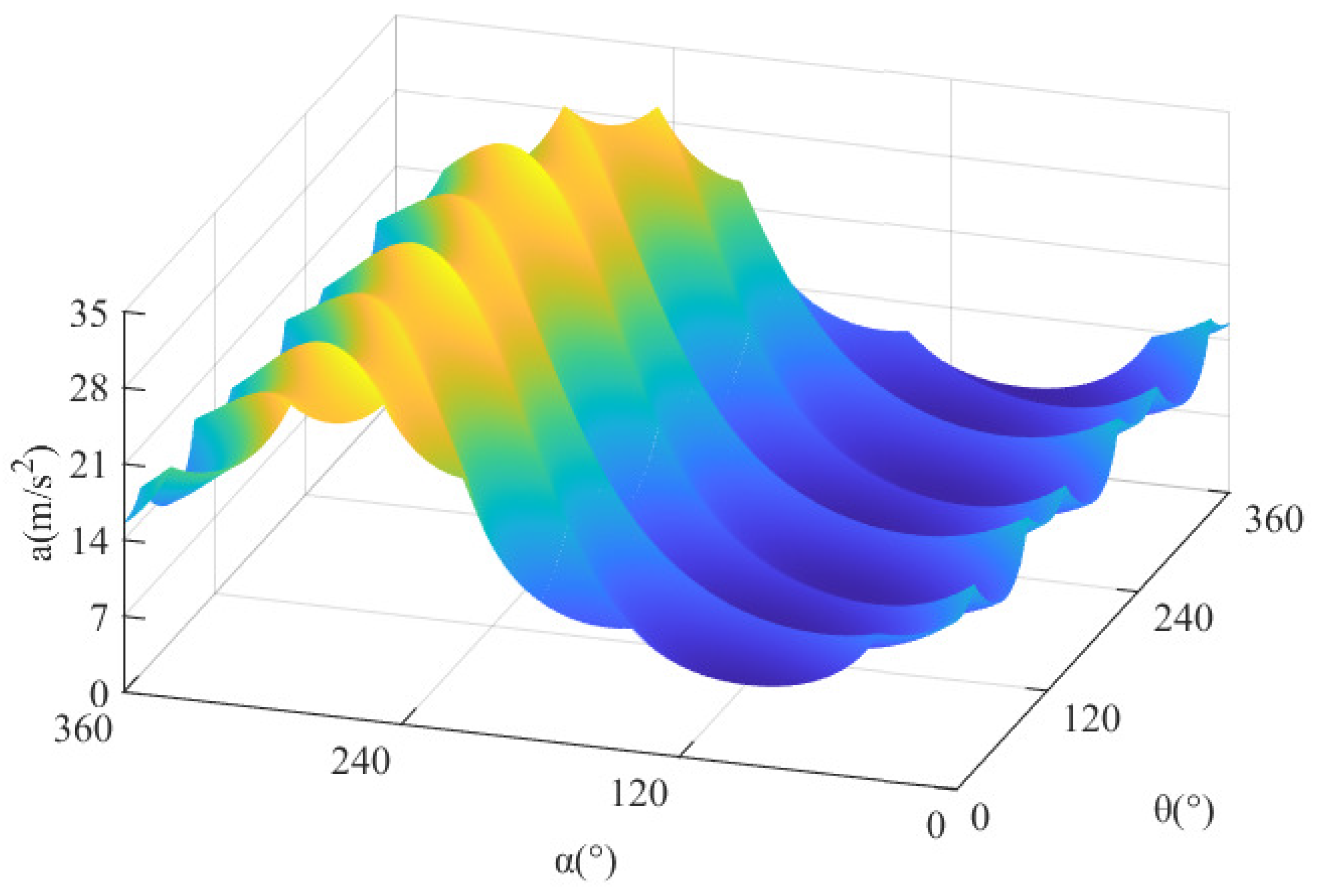
The translational acceleration a and corresponding orientation $\alpha$ where no slip occurs are determined by $a_x$ and $a_y$. The relationship can be expressed as follows.

$$\left\{\begin{array}{c}{a}_x=acos\alpha \hfill \\ a_y=asin\alpha \hfill \end{array}\right.$$

(12)

In the practical case, the physical model gives all the known physical parameters appearing in (7)–(12). Moreover, the relationship between $\theta$, $\alpha$, and $a_{max}$ under a non-slip state can be found. Assuming $m=2.615$ kg, $g=9.8$ m·s⁻², $M_G=1.314$ N·m, $r=0.2221$ m, ${\mu }_m=0.6$, and $F_A=150$ N, the relationship between $\theta$, $\alpha$, and $a_{max}$ is shown in Figure 5.

In Figure 5, the surface corresponds to the critical slip state, the space enclosed by the surface and the $\theta -\alpha$ plane is the achievable non-slip motion. In order to prevent the robot from slipping, without considering the influence of $\theta$ and $\alpha$ on the maximum acceleration, the minimum value of a on the surface in Figure 5 is usually taken as the constraint for the maximum value of the acceleration. Here, we have $a_{min}=7.31$ m·s⁻². Under the specific orientation and acceleration direction angle, the maximum acceleration of the robot is constrained to the maximum value of $a_{max}$ = 30.45 m·s⁻² on this surface. It can be seen that the maximum acceleration can be increased by $316.55\%$ by adjusting the maximum acceleration constraint in real time when considering the effect of the critical slip state. The average acceleration of the points on the surface in Figure 5 is $a_{avg}=19.35$ m·s⁻². It shows that the maximum acceleration is increased by $164.71\%$ on average when considering the influence of the critical slip state.

Similarly, for the rotational acceleration, we have

$$\left[\begin{array}{c}{F}_{w1}\\ F_{w2}\\ F_{w3}\end{array}\right]=\left[\begin{array}{ccc}-{\displaystyle \frac{2}{3}}sin(\theta +\pi )& {\displaystyle \frac{2}{3}}cos(\theta +\pi )& {\displaystyle \frac{1}{3r}}\\ -{\displaystyle \frac{2}{3}}sin(\theta -{\displaystyle \frac{\pi }{3}})& {\displaystyle \frac{2}{3}}sin(\theta -{\displaystyle \frac{\pi }{3}})& {\displaystyle \frac{1}{3r}}\\ -{\displaystyle \frac{2}{3}}sin(\theta +{\displaystyle \frac{\pi }{3}})& {\displaystyle \frac{2}{3}}sin(\theta -{\displaystyle \frac{\pi }{3}})& {\displaystyle \frac{1}{3r}}\end{array}\right]\left[\begin{array}{c}0\\ mg\\ I_z\ddot{\theta }\end{array}\right]$$

(13)

According to (13), when $\theta$ is fixed, the difference in the driving force of each wheel is fixed. Therefore, we have

$$\left\{\begin{array}{c}{F}_{w1}-F_{w2}=-{\displaystyle \frac{2\sqrt{3}mg}{3}}sin(\theta +{\displaystyle \frac{\pi }{3}})\hfill \\ F_{w2}-F_{w3}=-{\displaystyle \frac{2\sqrt{3}mg}{3}}sin(\theta +\pi )\hfill \\ F_{w3}-F_{w1}=-{\displaystyle \frac{2\sqrt{3}mg}{3}}sin(\theta -{\displaystyle \frac{\pi }{3}})\hfill \\ f_1=-{\displaystyle \frac{2{\mu }_m{M}_G}{3r}}sin(\theta +\pi )+{\displaystyle \frac{{\mu }_m{F}_A}{3}}\hfill \\ f_2=-{\displaystyle \frac{2{\mu }_m{M}_G}{3r}}sin(\theta -{\displaystyle \frac{\pi }{3}})+{\displaystyle \frac{{\mu }_m{F}_A}{3}}\hfill \\ f_3=-{\displaystyle \frac{2{\mu }_m{M}_G}{3r}}sin(\theta +{\displaystyle \frac{\pi }{3}})+{\displaystyle \frac{{\mu }_m{F}_A}{3}}\hfill \end{array}\right.$$

(14)

If $W_1$ reaches the maximum static friction first, we have

$$\left\{\begin{array}{c}{F}_{w1}=f_1\hfill \\ F_{w2}=f_1-(F_{w1}-F_{w2})\hfill \\ F_{w3}=(F_{w3}-F_{w1})+f_1\hfill \\ \beta ={\displaystyle \frac{3r(f_1-{\displaystyle \frac{2}{3}}mgcos(\theta +\pi ))}{I_z}}\hfill \end{array}\right.$$

(15)

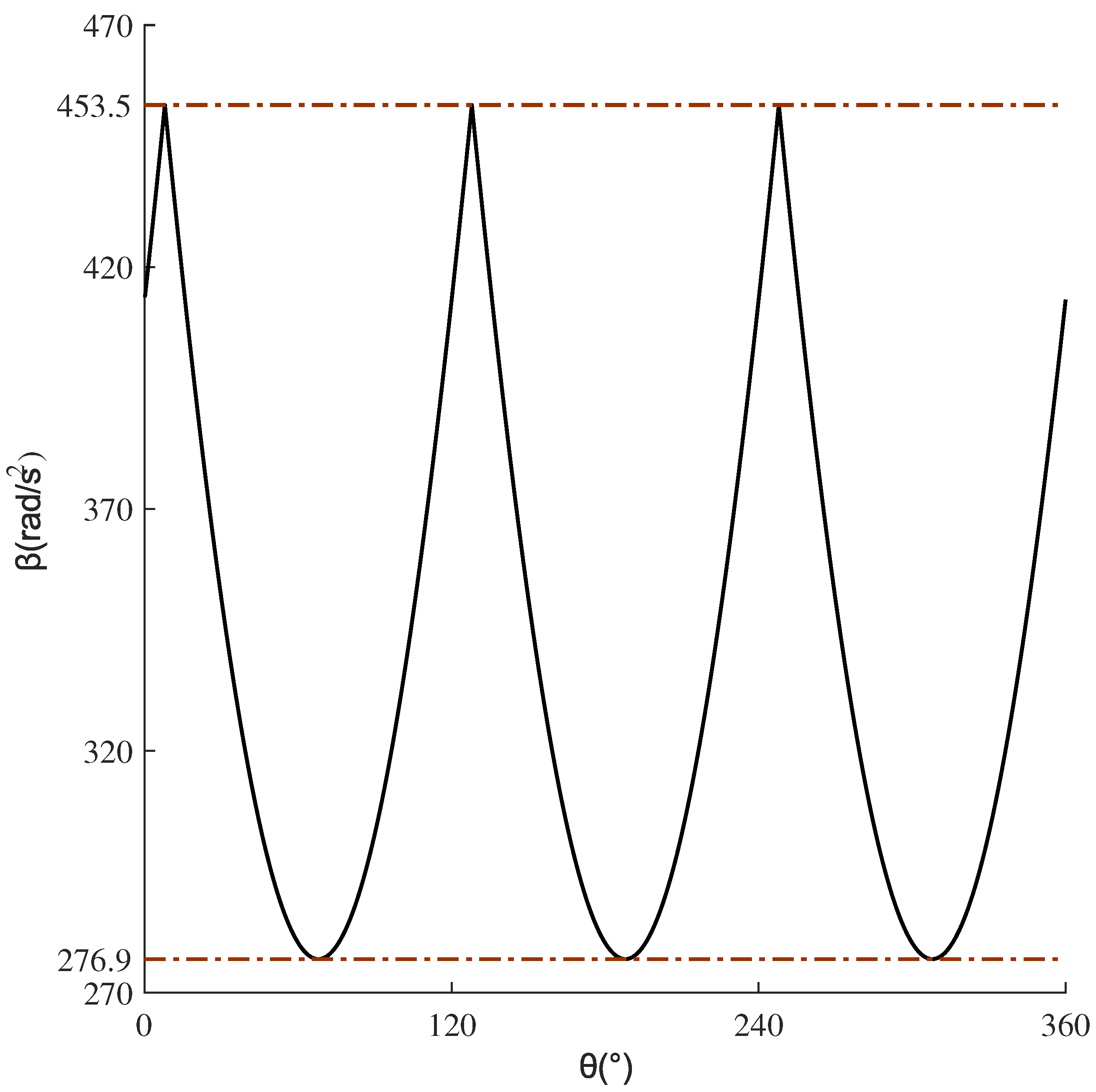
The same is true when $W_2$ or $W_3$ reaches the maximum static friction force first. The curve can be obtained as in Figure 6, which is the critical slip state parameter, and the region enclosed by this curve and $\theta$-axis is the motion state that can be achieved in the non-slip state. When the influence of the critical slip state is not considered, the minimum value of $\beta$ on the graph curve is usually taken as the constraint on the maximum value of the angular acceleration of the robot to prevent the robot from slipping. Here, we have ${\beta }_{min}=276.94$ rad·s⁻². Under the conditions of a specific $\theta$ and $\alpha$, the maximum acceleration of the robot is constrained to be the maximum value on this surface ${\beta }_{max}=453.48$ rad·s⁻². It can be seen that when the influence of the critical slip state is considered, the maximum acceleration of the robot can be increased by $63.75\%$ by adjusting the maximum acceleration constraint in real-time. The average acceleration of the points on the surface in Figure 6 is ${\beta }_{avg}=338.05$ rad·s⁻². It can be seen that the maximum acceleration of the robot is increased by $22.07\%$ on average when considering the influence of $\theta$ and $\alpha$ on the maximum acceleration.

From the above, when $\theta$ and $\gamma$ are given, the relation of $F_{wi}(i=1,2,3)$, a, and $\alpha$ can be found. The conclusion can be used to adjust the maximum acceleration according to $\theta$ and $\alpha$. The constraints on the maximum acceleration of the robot can be adjusted in real time to exploit the acceleration performance fully. When $\theta$ in the world coordinate system is given, the maximum angular acceleration $\beta$ of the robot in the world coordinate system can be found when the robot is in the critical slip state. The constraint on $\beta$ can be adjusted in real time according to $\theta$, so the acceleration performance of the system can be more fully exploited.

4. Nonlinear Model Predictive Trajectory Tracking Control

Trajectory tracking accuracy could be vital when a wall-climbing robot performs particular tasks in a real application. Traditional PID controllers are widely used in trajectory tracking control. However, the accuracy of the traditional PID controller is significantly impacted by delays of dynamic characteristics of the robot. Therefore, our robot’s trajectory tracking motion control is designed based on nonlinear model predictive control(NMPC). The kinematic equations of the system can be expressed as follows:

$$\dot{\mathbf{X}}=\left[\begin{array}{c}\dot{x}\left(t\right)\\ \dot{y}\left(t\right)\\ \dot{\theta }\left(t\right)\end{array}\right]\left[\begin{array}{ccc}-{\displaystyle \frac{2}{3}}sin(\theta \left(t\right)+\pi )& -{\displaystyle \frac{2}{3}}sin(\theta \left(t\right)-{\displaystyle \frac{\pi }{3}})& -{\displaystyle \frac{2}{3}}sin(\theta \left(t\right)+{\displaystyle \frac{\pi }{3}})\\ {\displaystyle \frac{2}{3}}cos(\theta \left(t\right)+\pi )& {\displaystyle \frac{2}{3}}cos(\theta \left(t\right)-{\displaystyle \frac{\pi }{3}})& {\displaystyle \frac{2}{3}}cos(\theta \left(t\right)+{\displaystyle \frac{\pi }{3}})\\ {\displaystyle \frac{1}{3r}}& {\displaystyle \frac{1}{3r}}& {\displaystyle \frac{1}{3r}}\end{array}\right]\left[\begin{array}{c}{v}_1\left(t\right)\\ v_2\left(t\right)\\ v_3\left(t\right)\end{array}\right]$$

(16)

where $\dot{\mathbf{X}}$ is the velocity state quantity of the robot, and $\dot{x}$ and $\dot{y}$ are the velocity component of the robot’s motion on the X-axis and Y-axis of the world coordinate system, respectively. $\dot{\theta }$ is the angular velocity around the center of the robot coordinate system. Velocities $v_1$, $v_2$, and $v_3$ are the relative motion velocities of the three wheels to the wall, respectively.

The dynamic equations of the system can be expressed as follows.

$$\ddot{\mathbf{X}}=\left[\begin{array}{c}\ddot{x}\left(t\right)\\ \ddot{y}\left(t\right)\\ \ddot{\theta }\left(t\right)\end{array}\right]\left[\begin{array}{ccc}{\displaystyle \frac{-sin\left(\theta \right(t)+\pi )}{m}}& {\displaystyle \frac{-sin(\theta \left(t\right)-{\displaystyle \frac{\pi }{3}})}{m}}& {\displaystyle \frac{-sin(\theta \left(t\right)+{\displaystyle \frac{\pi }{3}})}{m}}\\ {\displaystyle \frac{sin\left(\theta \right(t)+\pi )}{m}}& {\displaystyle \frac{sin(\theta \left(t\right)-{\displaystyle \frac{\pi }{3}})}{m}}& {\displaystyle \frac{sin(\theta \left(t\right)+{\displaystyle \frac{\pi }{3}})}{m}}\\ {\displaystyle \frac{r}{I_z}}& {\displaystyle \frac{r}{I_Z}}& {\displaystyle \frac{r}{I_Z}}\end{array}\right]\left[\begin{array}{c}{F}_{w1}\left(t\right)\\ F_{w2}\left(t\right)\\ F_{w3}\left(t\right)\end{array}\right]+\left[\begin{array}{c}0\\ -g\\ 0\end{array}\right]$$

(17)

where $\ddot{\mathbf{X}}$ is the acceleration state quantity of the robot, and $\ddot{x}$ and $\ddot{y}$ are the acceleration component of the robot’s motion on the X-axis and Y-axis of the world coordinate system, respectively. $\ddot{\theta }$ is the angular acceleration around the center $O^{\prime }$ of the robot coordinate system. The final control quantity of the robot is the driving force of each wheel of the robot. Moreover, the relationship between the velocity state and acceleration state can be expressed as follows:

$$\ddot{\mathbf{X}}\left(t\right)=f(\dot{\mathbf{X}}\left(t\right),\mathbf{u}\left(t\right))$$

(18)

where

$$\mathbf{u}\left(t\right)=\left[\begin{array}{c}{u}_1\left(t\right)\\ u_2\left(t\right)\\ u_3\left(t\right)\end{array}\right]=\left[\begin{array}{c}{F}_{w1}\left(t\right)\\ F_{w2}\left(t\right)\\ F_{w3}\left(t\right)\end{array}\right]$$

(19)

For a given reference trajectory, each point on the trajectory satisfies the kinematic and dynamic equations described by (16) and (17). The reference quantity is denoted by the subscript r. Then, we have

$${\ddot{\mathbf{X}}}_r\left(t\right)=f({\dot{\mathbf{X}}}_r\left(t\right),{\mathbf{u}}_r\left(t\right))$$

(20)

where

$$\left\{\begin{array}{c}{\dot{\mathbf{X}}}_r=\left[\begin{array}{c}{\dot{x}}_r\left(t\right)\\ {\dot{y}}_r\left(t\right)\\ {\dot{\theta }}_r\left(t\right)\end{array}\right]\hfill \\ {\mathbf{u}}_r\left(t\right)=\left[\begin{array}{c}{u}_{r1}\left(t\right)\\ u_{r2}\left(t\right)\\ u_{r3}\left(t\right)\end{array}\right]=\left[\begin{array}{c}{F}_{rw1}\left(t\right)\\ F_{rw2}\left(t\right)\\ F_{rw3}\left(t\right)\end{array}\right]\hfill \end{array}\right.$$

(21)

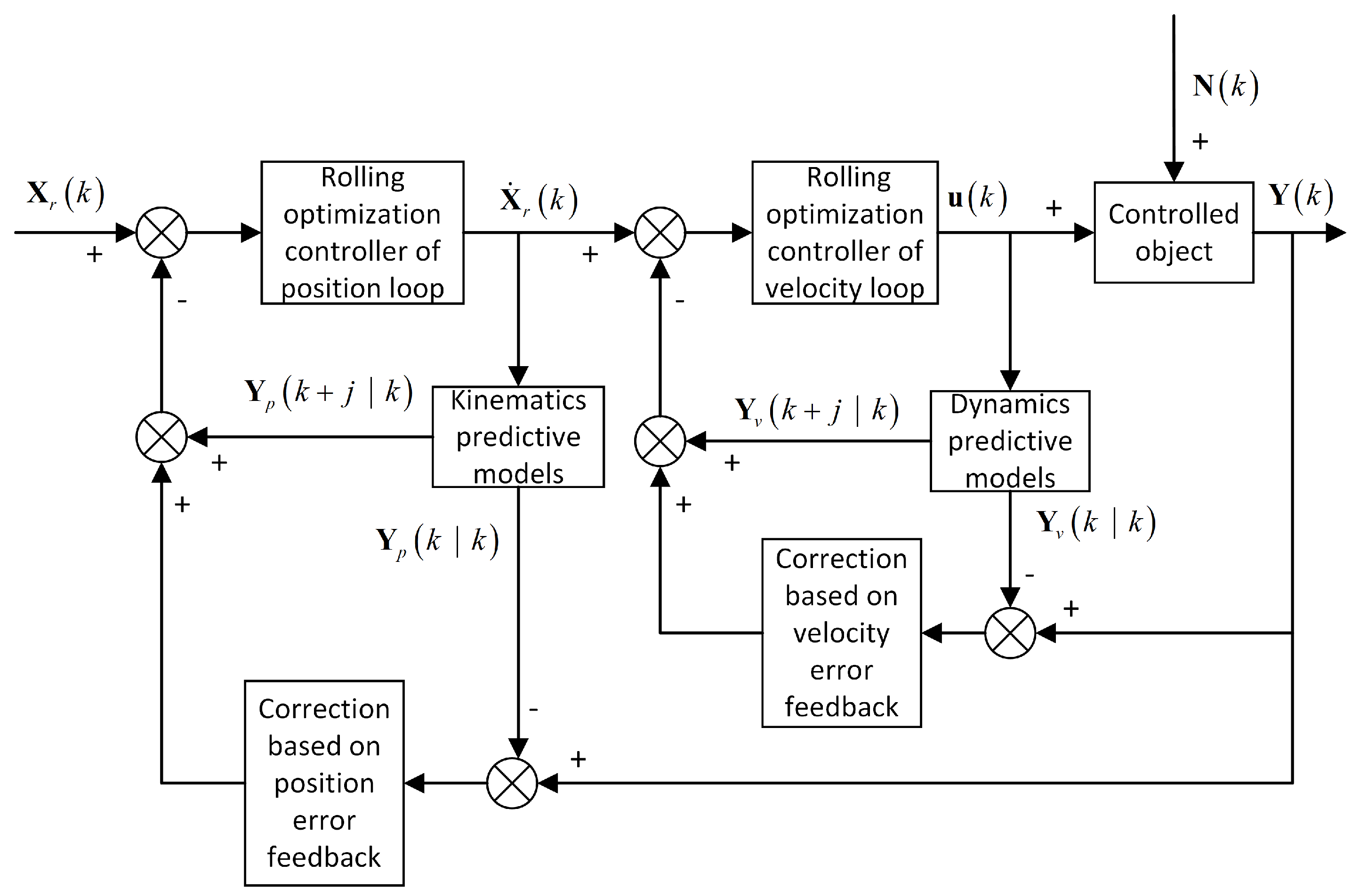
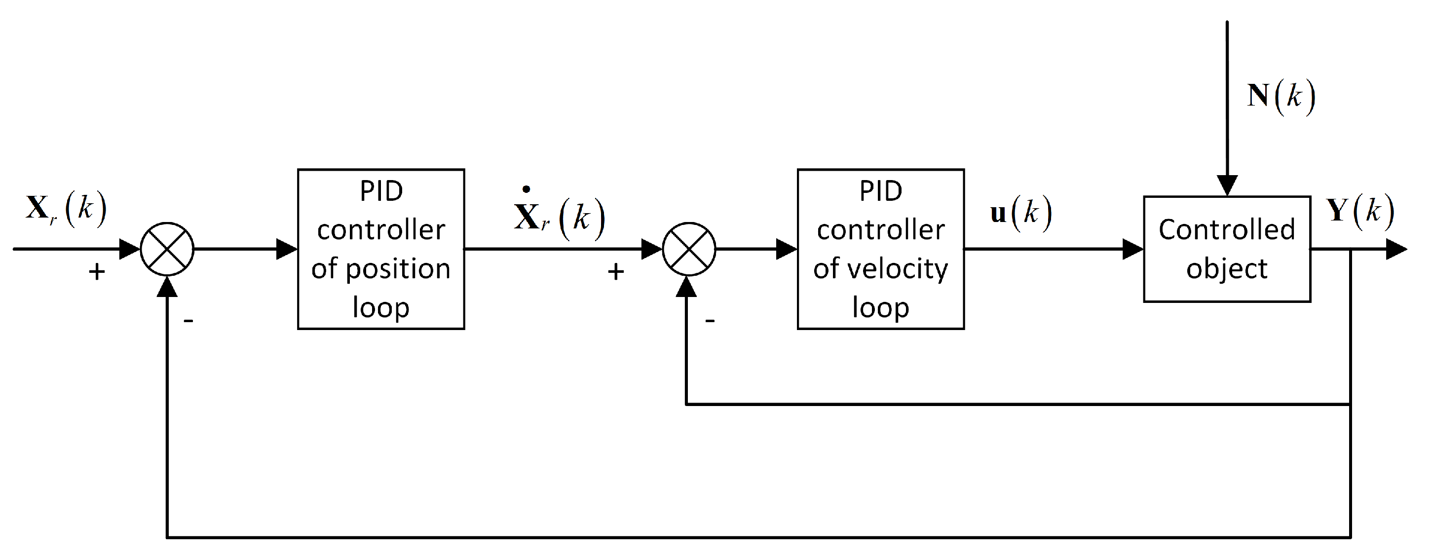
In order to obtain a better control effect, a model predictive controller with a dual-loop structure including position and velocity loops is designed in this paper, as shown in Figure 7. The control quantity calculated by the position loop is the velocity of the robot in the world coordinate system. It is then used as the reference quantity of the velocity loop. Therefore, the position loop is calculated to obtain its error prediction model.

According to the sampling theorem, when the number of prediction steps is n, the discretization of the $\mathbf{X}$ can be expressed as follows:

$${\mathbf{X}}_e(k+n|k)=\mathbf{X}\left(k\right|k)+T\sum _{i=1}^n{\dot{\mathbf{X}}}_r(k+i-1|k)-{\mathbf{X}}_r(k+n|k)$$

(22)

where ${\mathbf{X}}_r(k+n|k)$ is a vector of position state quantities of the reference trajectory after the time $nT$, input to the controller from higher-level decisions such as trajectory planning in the robot. Vector ${\dot{\mathbf{X}}}_r(k+i-1|k)$ is the velocity state volume vector of the reference trajectory of the robot after the time $(i-1)T$, which is the control volume of the position loop and calculated by the position loop’s optimization controller and input to the velocity loop as the reference trajectory of the velocity loop.

In this paper, an objective function is designed, which considers the accuracy of trajectory tracking, smoothness of motion control, and solvability of the optimization algorithm [34] of the robot, and its expression form is as follows:

$$J\left(k\right)=\sum _{i=1}^{N_p}{\left|\left|{\dot{\mathbf{X}}}_e(k+i|k)\right|\right|}_{\mathbf{Q}}^2+\sum _{i=1}^{N_c}{\left|\left|\Delta \mathbf{u}(k+i|k)\right|\right|}_{\mathbf{R}}^2+{\left|\left|{\epsilon }_v\right|\right|}_{\rho }^2$$

(23)

where $J\left(k\right)$ is the optimization objective function, $\mathbf{Q}$ and $\mathbf{R}$ are the weight matrices, $\epsilon$ is the relaxation factor, $\rho$ is the relaxation factor weight coefficient, $N_p$ is the number of prediction steps, and $N_c$ is the number of control steps, with $N_p\ge N_c$. We have

$$\Delta \mathbf{u}(k+i|k)=\mathbf{u}(k+i\left|k\right)-\mathbf{u}(k+i-1|k)$$

(24)

where $k=1,2,3,\cdots ,N_c-1$.

This is considering the fact that the critical slip state into the constraint can fully utilize the robot’s motion performance because no undesired slip occurs. Based on the conclusions related to the critical slip state, the constraints are adjusted according to the specific needs of the NMPC algorithm. In practical applications, if the robot is in a critical slip state for a long time, its motion will be unstable and eventually lead to undesired slip. Similarly, if the robot’s drive motor is at full load for a long time, it may lead to high current, motor heating, and a decrease in the drive torque that the motor can provide, which may cause the motor to block. Therefore, a safety factor is designed for the constraints aiming at real-life problems to ensure that the robot will not be in a critical slip state and the motors will not be fully loaded for a long time.

With the introduction of the safety factor, the constraints of the velocity loop are

$$\left\{\begin{array}{c}\left|\mathbf{u}(t+kT)\right|\le {\mathbf{S}}_f\mathbf{f}(t+kT)\hfill \\ \left|\mathbf{u}(t+kT)\right|\le {\mathbf{S}}_w{\mathbf{F}}_{wmax}\hfill \end{array}\right.$$

(25)

where ${\mathbf{S}}_f$ and ${\mathbf{S}}_w$ are the safety coefficient matrices.

For the position loop, the constraint mainly lies in the fact that the tangential relative motion speed between each wheel and the wall should not exceed the linear speed that the motor can provide for each wheel. Otherwise, the undesired slip between the wheel and the wall will occur. Thus, for the position loop, we have

$${\mathbf{S}}_v{\mathbf{v}}_{min}\le \mathbf{A}(t+kT)\dot{\mathbf{X}}(t+kT)\le {\mathbf{S}}_v{\mathbf{v}}_{max}$$

(26)

where ${\mathbf{S}}_v$ is the safety coefficient matrix, and

$$\mathbf{A}(t+kT)=\left[\begin{array}{ccc}-sin\left(\theta \right(t+kT)+\pi )& cos\left(\theta \right(t+kT)+\pi )& r\\ -sin(\theta (t+kT)-{\displaystyle \frac{\pi }{3}})& cos(\theta (t+kT)-{\displaystyle \frac{\pi }{3}})& r\\ -sin(\theta (t+kT)+{\displaystyle \frac{\pi }{3}})& cos(\theta (t+kT)-{\displaystyle \frac{\pi }{3}})& r\end{array}\right]$$

(27)

5. Simulation Experiments

In this paper, the dynamics simulation software ADAMS is used to model the dynamics of the robot to verify the derived positive pressure model of each wheel on the wall and the model of the critical slip state. In the simulation experiments, we consider the contact deformation and the dimensional parameters of the model. The type of material and its physical parameters in the experiments are the same as the mechanism design. Here we have $m=2.615$ kg, $h=51.27$ mm, $F_A=150$ N, and $r=222.1$ mm.

5.1. Critical Slip State Experiments

In the critical slip state experiment, three states of non-slip, critical slip, and slip were analyzed. The control signal is a step signal fed directly to the wheel. In the critical slip state experiments, we have no constraints on the performance of the motor in the simulation environment. For $\theta ={90}^{\circ }$ and $\alpha =0^{\circ }$, the theoretical acceleration values were compared with the simulated experimental values in the three states.

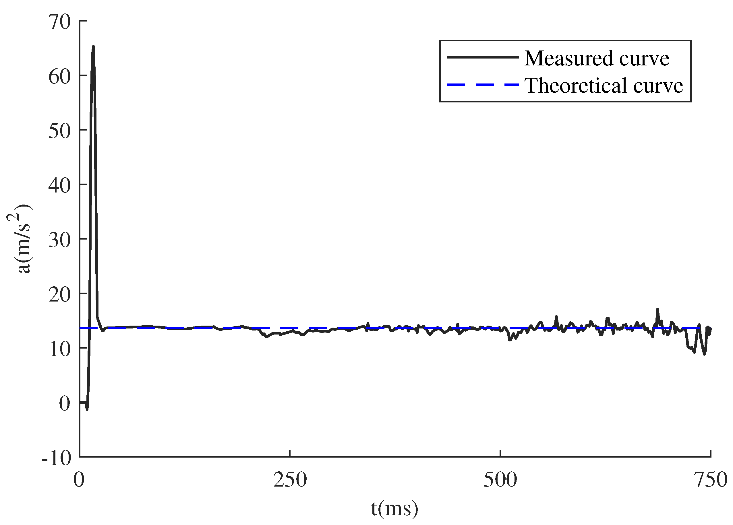
Figure 8 shows the measured acceleration and theoretical acceleration curves of the robot in the simulation experiment when the driving force of $W_1$, $W_2$, and $W_3$ are $23.76$ N, $2.91$ N, and $-26.67$ N, respectively. The robot is in a non-slip state in this case. It can be seen that the theoretical acceleration curve in the figure is consistent with the acceleration measured in the simulation experiment. The pulse at 15 ms in the graph is generated by the shock caused by the system starting from a standstill.

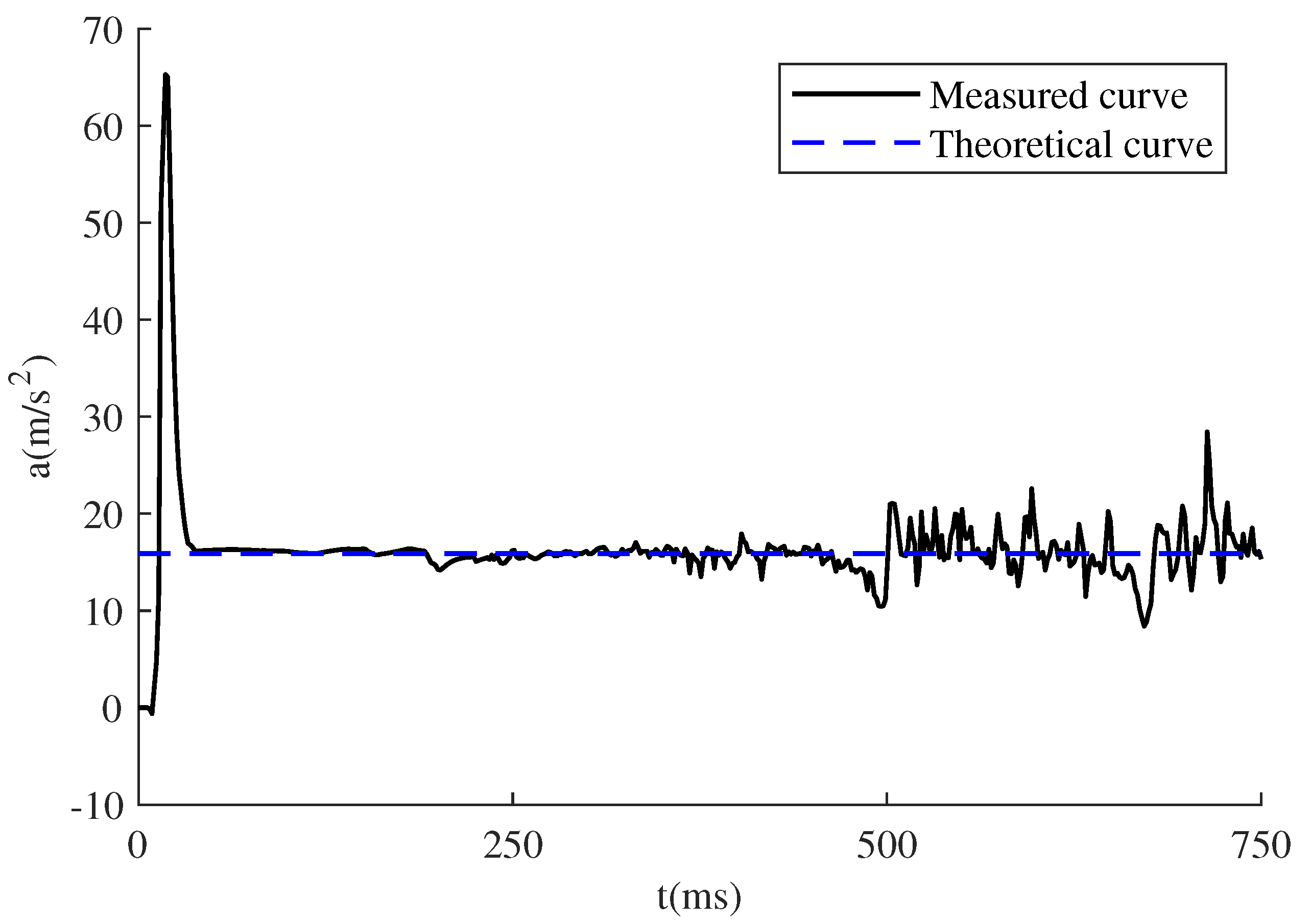
Figure 9 shows the measured acceleration and theoretical acceleration curves of the robot in the simulation experiment when the driving force of $W_1$, $W_2$, and $W_3$ are $28.02$ N, $0.80$ N, and $-28.82$ N, respectively. In this case, the robot is in the critical slip state. It can be seen that the acceleration theoretical value curve in the figure is consistent with the acceleration measured in the simulation experiment. The pulse at 17 ms in the figure is generated by the shock caused by the system starting from rest. The oscillation after 500 ms is caused by an unstable form of friction. The wheel speed is already high at this time, and the omnidirectional wheel rollers make contact with the wall one after another, resulting in the unstable form of friction.

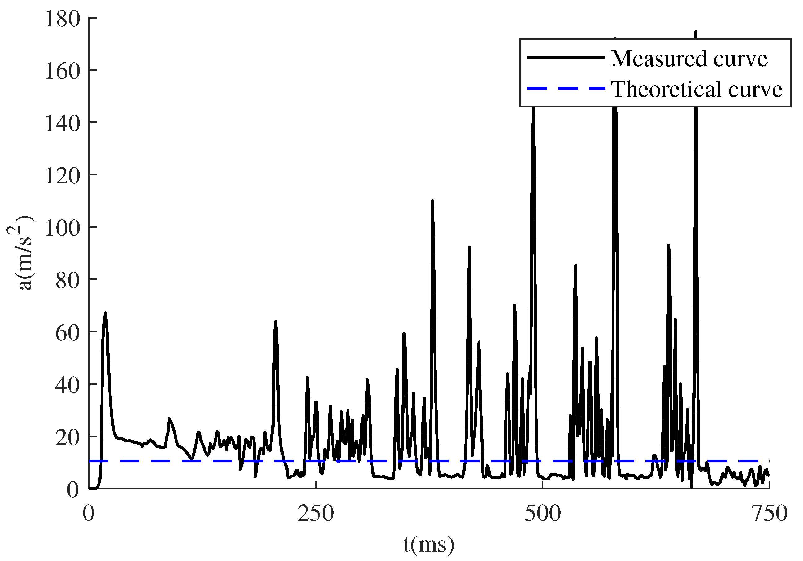
Figure 10 shows the measured acceleration and theoretical acceleration curves of the robot in the simulation experiment when the driving forces of $W_1$, $W_2$, and $W_3$ are $31.68$ N, $-1.05$ N, and $-30.63$ N, respectively. The robot is slipping in this case. It can be seen that the acceleration theoretical value curve in the figure differs significantly from the acceleration measured in the simulation experiment. The difference is due to the oscillation of acceleration as the omnidirectional wheel rotates, generating sliding friction and slipping. The rollers of the omnidirectional wheel are in alternating contact with the wall, which causes the oscillation. The oscillation here is more evident than the non-slip state and the critical slip state, which is not suitable for the stable control of the robot, so the undesired slip of the omnidirectional wheel with the wall should be avoided.

From the three experiments above, it can be seen that according to the critical slip state model in Section 3.2, the drive force can be accurately calculated for the system to accelerate in any direction without changing $\theta$ in the non-slip state and the critical slip state.

5.2. Control Algorithm Experiments

To verify the performance of our NMPC controller, we have completed experiments using the NMPC controller and the PID controller as a comparison. The simulated solvers are all fixed-step types with 5 ms step. In addition, a time delay of 5 ms is added to the feedback link to simulate the sensor communication time delay in real applications.

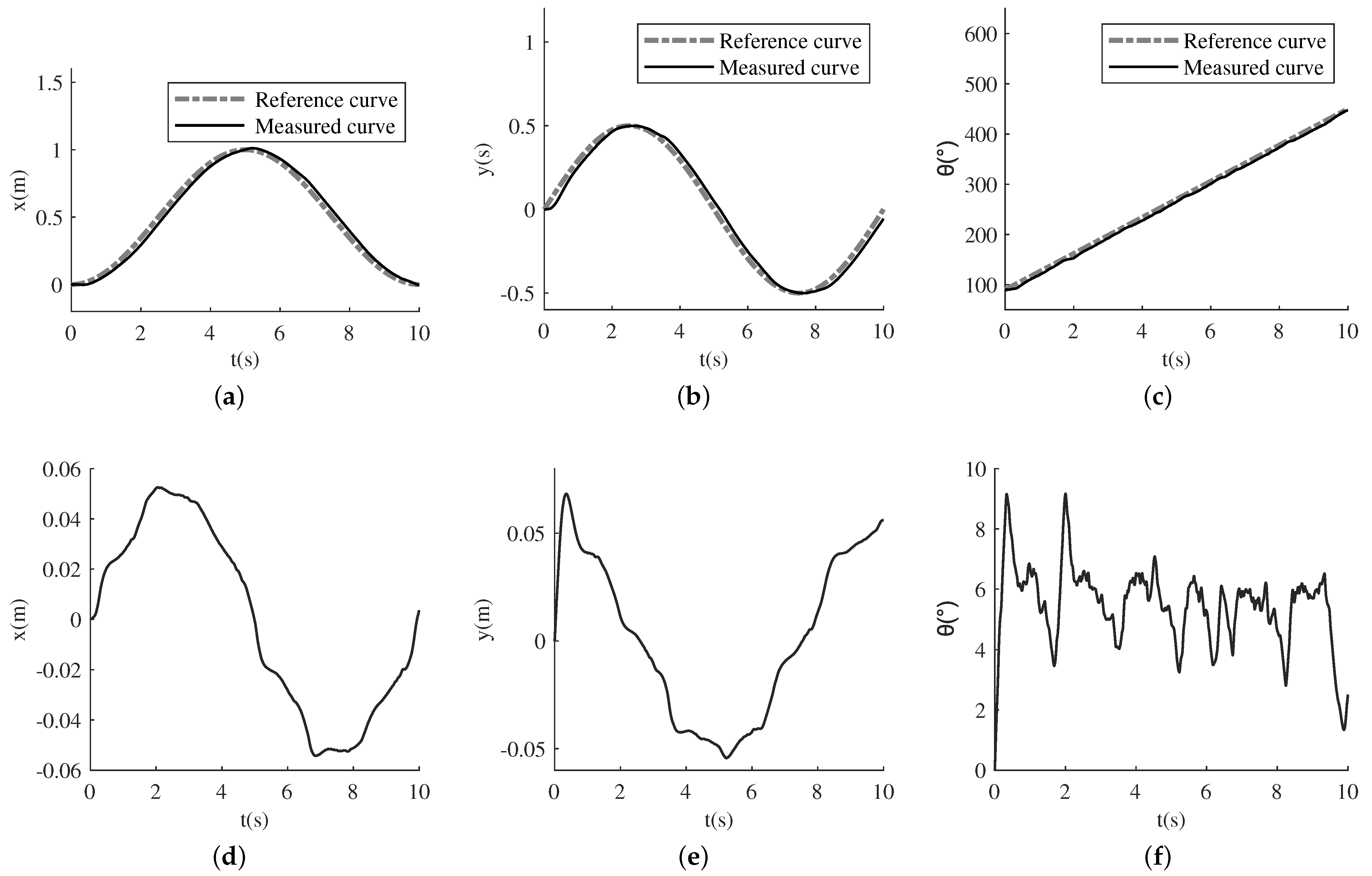
The dual-loop structure of the PID controller in the simulation experiments is shown in Figure 11, and the structure of $K_p$, $K_i$, and $K_d$ is used in the calculation. The PID parameters corresponding to the error values of X-direction, Y-direction, and rotation direction of the position loop are $7,0.1,$ and $0.1$, respectively. The PID parameters corresponding to the error values of the X-direction and Y-direction of the velocity loop are $7,0.1,$ and 0, respectively. The PID parameters for the error values of rotation angle velocity are $14,0.1,$ and 0. The PID parameters are selected through experimental tests. First, the PID parameters is empirically adjusted so that the robot can roughly follow the trajectory in X-direction, Y-direction and orientation. Then, the parameters of the inner loop are tuned in the order of $K_p$, $K_i$, and $K_d$, followed by the outer loop in the same tuning order. The parameter step of $K_p$ is 0.5 and the parameter step of $K_i$ and $K_d$ is 0.1. Next, when the robot’s trajectory is close to the reference trajectory, we compare the RMSE of the trajectory tracking. Finally, the parameters with the smallest sum of the RMSE in the three dimensions. The result shown in the paper is the local best performance obtained from numerical experiments. The lower bound of the constraint of the position loop is ${\left[\begin{array}{ccc}-0.32& -0.32& -70\end{array}\right]}^T$, and the upper bound is ${\left[\begin{array}{ccc}0.32& 0.32& 70\end{array}\right]}^T$. The lower bound of the constraint of the velocity loop is ${\left[\begin{array}{ccc}-50& -50& -50\end{array}\right]}^T$, and the upper bound is ${\left[\begin{array}{ccc}50& 50& 50\end{array}\right]}^T$. The constraints’ parameters are calculated from the physical constraints. The experimental results are shown in Figure 12.

The parameters of the experimentally measured trajectory in Figure 12 do not overlap with those of the reference trajectory. As a result, the experimentally measured trajectories of the position in the X-direction, Y-direction, and the orientation have a slight time delay compared with the reference trajectory.

In the simulation experiments using the NMPC algorithm, the number of prediction steps is 1 and the number of control steps is 1.

The control frequency of the position loop is 20 Hz, and the control frequency of the velocity loop is 200 Hz. The parameters of the prediction and control horizons are set for control frequency and model accuracy reasons. According to (22), the computation of the difference model increases significantly when the prediction and control horizons increase. Moreover, to simplify the calculation, $\theta$ is replaced by ${\theta }_r$ in the model, so the model mismatch is also more severe when the prediction and control horizons increase. It has been tested that when the prediction and control horizons are 1, the controller can reach the maximum control frequency with no decrease in accuracy. The tracking accuracy penalty matrix of the position loop can be expressed as follows:

$${\mathbf{Q}}_p=\left[\begin{array}{ccc}100,000& 0& 0\\ 0& 100,000& 0\\ 0& 0& 10,000\end{array}\right]$$

The control smoothness penalty matrix of the position loop is

$${\mathbf{R}}_p=\left[\begin{array}{ccc}0.01& 0& 0\\ 0& 0.01& 0\\ 0& 0& 0.001\end{array}\right]$$

The relaxation factor coefficient of the position loop is

$${\rho }_p=0$$

The tracking accuracy penalty matrix of the velocity loop is

$${\mathbf{Q}}_v=\left[\begin{array}{ccc}270,000& 0& 0\\ 0& 270,000& 0\\ 0& 0& 900\end{array}\right]$$

The control smoothness penalty matrix for the velocity loop is

$${\mathbf{R}}_v=\left[\begin{array}{ccc}0.01& 0& 0\\ 0& 0.01& 0\\ 0& 0& 10,000\end{array}\right]$$

The relaxation factor coefficient of the velocity loop is

$${\rho }_v=0$$

The safety coefficient vector ${\mathbf{S}}_f$, ${\mathbf{S}}_w$ and ${\mathbf{S}}_v$ are all taken as ${\left[\begin{array}{ccc}0.95& 0.95& 0.95\end{array}\right]}^T$.

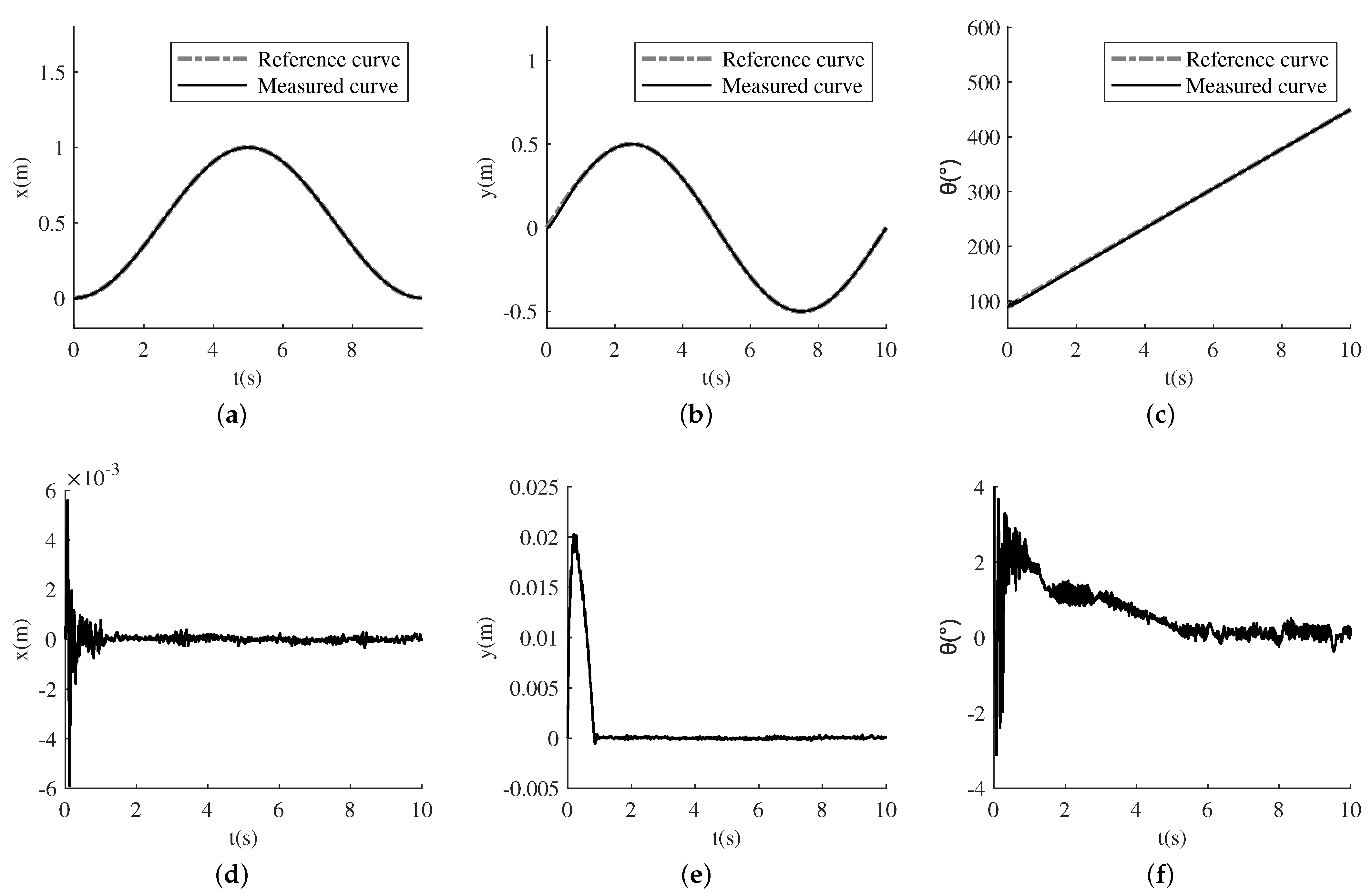
The results of the simulation experiment are shown in Figure 13. The experimental measurement trajectories in the experimental results overlap with the reference trajectory. Compared with the PID algorithm, the NMPC algorithm reduces the impact of time delay on control accuracy. The NMPC controller achieves accurate and smooth trajectory tracking control of the robot during the wall motion.

In order to further quantify and compare the tracking accuracy of the PID algorithm and NMPC algorithm, we use the root mean square error (RMSE) between the experimentally measured trajectory position quantity and the reference trajectory position quantity as the evaluation index. The comparison results are shown in

Table 1. Comparison of the RMSE of PID experiment and NMPC experiment.

Program	RMSE for X-Directional Position	RMSE for Y-Directional Position	RMSE for Orientation
PID experiment results	$3.661\times {10}^{-2}$	$3.684\times {10}^{-2}$	$1.219$
NMPC experiment results	$4.946\times {10}^{-4}$	$3.839\times {10}^{-3}$	$4.844\times {10}^{-1}$

.

From the results in Table 1, the RMSE of PID experimental results in X-direction and Y-direction position quantities are approximately $74.02$ times and $9.596$ times of NMPC experimental results, respectively, while the ratio of RMSE of PID experimental results to NMPC experimental results in terms of orientation is $2.516$. Thus, the results indicate that the deviation of the actual trajectory and the reference trajectory of the NMPC algorithm is smaller than that of the PID algorithm in the joint dynamics simulation environment. Therefore, the NMPC algorithm outperforms the PID algorithm in terms of trajectory tracking accuracy in the application scenario of this paper.

6. Discussion and Future Work

As the omnidirectional wheels rotate, the alternating forces on the rollers create a cyclic shock. The shock causes a periodic change in the positive pressure between each robot wheel and the wall. Therefore, when the robot is in a critical slip state, this shock eventually leads to unstable friction between the robot’s wheels and the wall, thus causing the oscillation after 500 ms in Figure 9. According to the description in [35], this shock can be reduced by adjusting the omnidirectional wheel form. As a result, the motion performance of the robot can be more fully exploited. The next step can be to improve the design of the omnidirectional wheel based on this requirement and complete the real robot.

In this paper, an NMPC algorithm is designed that is more accurate than the linear MPC algorithm model but still suffers from the model mismatch. In the experiments, the angle information in this model directly selects the angle of the reference trajectory instead of the prediction angle. If the angle of the reference trajectory is used, the prediction model mismatch will be aggravated when the robot’s orientation tracking is inaccurate; if the prediction angle is used, the computation of the prediction model will increase significantly as the number of predictions steps increases. Making the prediction model more accurate while ensuring the efficiency of the algorithm is an important research element to enhance this control algorithm. One possible solution to the problem of model mismatch is to use a data-driven nonlinear model. Parameter adaption techniques are often integrated into the MPC algorithm. Model predictive control based on the data-driven model as the neural network-based model predictive control(NNMPC) [36] and the Bayesian neural networks model predictive control(BNN-MPC) [37] are now widely researched and used.

Because of the favorable results of this simulation, the next step would be to implement this NMPC-based control algorithm on a real robot to test and compare the efficacy with the simulation results. Further theoretical research and engineering implementation are proceeding in parallel now. However, the conditions for experiments on a real robot are not available yet. There are many differences between real-life implementation and simulation that need to be addressed. For example, in real-life, the delay of the robot is unstable due to many factors, such as the hardware and environment. In addition, the accuracy of motion control is reduced because of perturbations in the robot’s attachment and drive forces. These problems make it challenging for the disturbance rejection of the control algorithm.

7. Conclusions

In this paper, a novel omnidirectional mobile pneumatic adhesion wall-climbing robot is designed, its dynamics model is derived, and the critical slip state is proposed. The dynamics constraint is given when considering the critical slip state, giving the robot fuller play to its motion performance. Its maximum acceleration can be improved by $164.71\%$ on average when the robot only has translational acceleration. The maximum angular acceleration can be improved by $22.07\%$ on average when the robot is only accelerated by rotation. Based on the dynamics model of this robot, a nonlinear model predictive trajectory tracking control algorithm is designed, and better control performance can be achieved in comparison with the PID algorithm in trajectory tracking. Using the RMSE of the measured trajectory and the reference trajectory as the criterion to evaluate the trajectory tracking accuracy, the accuracy of our algorithm is $74.02$ times that of the PID algorithm in the X-direction position, $9.596$ times in the Y-direction position, and $2.516$ times in the orientation.

References

- Xu, S.; He, B.; Hu, H. Research on Kinematics and Stability of a Bionic Wall-Climbing Hexapod Robot. Appl. Bionics Biomech. 2019, 2019, 6146214. [Google Scholar] [CrossRef]
- Liu, Y.; Sun, S.; Wu, X.; Mei, T. A Wheeled Wall-Climbing Robot with Bio-Inspired Spine Mechanisms. J. Bionic Eng. 2015, 12, 17–28. [Google Scholar] [CrossRef]
- Gradetsky, V.G.; Knyazkov, M.M. Multi-functional Wall Climbing Robot. In Proceedings of the 15th International Conference on Climbing and Walking Robots, Baltimore, MD, USA, 23–26 July 2012; pp. 807–812. [Google Scholar]
- Yamamoto, S. Development of inspection robot for nuclear pover plant. In Proceedings of the Proceedings 1992 IEEE International Conference on Robotics and Automation, Nice, France, 12–14 May 1992; pp. 1559–1566. [Google Scholar]
- Fan, J.; Xu, T.; Fang, Q.; Zhao, J.; Zhu, Y. A Novel Style Design of a Permanent-Magnetic Adsorption Mechanism for a Wall-Climbing Robot. J. Mech. Robot. Trans. ASME 2020, 12, 035001. [Google Scholar] [CrossRef]
- Sinkar, A.A.; Pandey, A.; Mehta, C. Design and Development of wall climbing Hexapod Robot with SMA actuated suction gripper. Procedia Comput. Sci. 2018, 133, 222–229. [Google Scholar] [CrossRef]
- Navaprakash, N.; Ramachandraiah, U.; Muthukumaran, G. Modeling and Experimental Analysis of Suction Pressure Generated by Active Suction Chamber Based Wall Climbing Robot with a Novel Bottom Restrictor. Procedia Comput. Sci. 2018, 133, 847–854. [Google Scholar]
- Fan, J.; Xu, T.; Fang, Q.; Zhao, J.; Zhu, Y. Fluid Model of Sliding Suction Cup of Wall-climbing Robots. Int. J. Adv. Robot. Syst. 2008, 3, 275–284. [Google Scholar]
- Liu, J.; Xu, L.; Chen, H. Development of a Bio-Inspired Wall-Climbing Robot Composed of Spine Wheels, Adhesive Belts and Eddy Suction Cup. Robotica 2021, 39, 3–22. [Google Scholar] [CrossRef]
- Xu, F.; Wang, B.; Shen, J. Design and Realization of the Claw Gripper System of a Climbing Robot. J. Intell. Robot. Syst. 2017, 89, 1–17. [Google Scholar] [CrossRef]
- Boomeri, V.; Tourajizadeh, H. Design, Modeling, and Control of a New Manipulating Climbing Robot Through Infrastructures Using Adaptive Force Control Method. Robotica 2020, 38, 2039–2059. [Google Scholar] [CrossRef]
- Xu, F.; Meng, F.; Jiang, Q. Grappling claws for a robot to climb rough wall surfaces: Mechanical design, grasping algorithm, and experiments. Robot. Auton. Syst. 2020, 128, 103501. [Google Scholar] [CrossRef]
- Liu, Y.; Seo, T.W. AnyClimb-II: Dry-adhesive linkage-type climbing robot for uneven vertical surfaces. Mech. Mach. Theory 2018, 124, 197–210. [Google Scholar] [CrossRef]
- Schmidt, D.; Berns, K. Climbing Robots for Maintenance and Inspections of Vertical Structures—A Survey of Design Aspects and Technologies. Robot. Auton. Syst. 2013, 61, 1288–1305. [Google Scholar] [CrossRef]
- Nansai, S.; Mohan, R.E. A Survey of Wall Climbing Robots: Recent Advances and Challenges Robotics. Robotics 2016, 5, 14. [Google Scholar] [CrossRef] [Green Version]
- Tavakoli, M.; Viegas, C.; Marques, L. OmniClimbers: Omni-directional magnetic wheeled climbing robots for inspection of ferromagnetic structures. Robot. Auton. Syst. 2013, 61, 997–1007. [Google Scholar] [CrossRef] [Green Version]
- Tang, X.; Zhang, D.; Li, Z. An Omni-Directional Wall-Climbing Microrobot with Magnetic Wheels Directly Integrated with Electromagnetic Micromotors. Int. J. Adv. Robot. Syst. 2012, 9, 16. [Google Scholar] [CrossRef]
- L, J.; Wang, X.S. Novel Omnidirectional Climbing Robot with Adjustable Magnetic Adsorption Mechanism. In Proceedings of the 2016 23rd International Conference on Mechatronics and Machine Vision in Practice (M2VIP), Nanjing, China, 28–30 November 2016; pp. 1–5. [Google Scholar]
- Schmidt, D.; Berns, C. Improving Navigation Safety of an Omni-Directional Wall-Climbing Robot via Traction and Friction Control. Trans. Control. Mech. Syst. 2014, 3, 36–43. [Google Scholar]
- Kuo, C.H.; Chou, H.C.; Chernousko, F.L. Trajectory Tracking of a Wheeled Wall Climbing Robot Using PID Controller. In Proceedings of the 2015 International Conference on Advanced Mechatronics, Intelligent Manufacture, and Industrial Automation (ICAMIMIA), Surabaya, Indonesia, 15–17 October 2015; pp. 143–146. [Google Scholar]
- Liu, X.; Wang, W.; Li, X. MPC-Based High-Speed Trajectory Tracking for 4WIS Robot. ISA Trans. 2016, 143–146. [Google Scholar] [CrossRef]
- He, N.; Li, L.Q.R. Design of a Model Predictive Trajectory Tracking Controller for Mobile Robot Based on the Event-Triggering Mechanism. Math. Probl. Eng. 2021, 12, 1–13. [Google Scholar] [CrossRef]
- Zhu, D.; Du, B.; Zhu, P. Adaptive Backstepping Sliding Mode Control of Trajectory Tracking for Robotic Manipulators. Complexity 2020, 2020, 3156787. [Google Scholar]
- Park, B.; Yoo, S.; Park, J. A Simple Adaptive Control Approach for Trajectory Tracking of Electrically Driven Nonholonomic Mobile Robots. IEEE Trans. Control. Syst. Technol. 2010, 18, 1199–1206. [Google Scholar] [CrossRef]
- Chen, Z.; Liu, Y.; He, W. Adaptive-Neural-Network-Based Trajectory Tracking Control for a Nonholonomic Wheeled Mobile Robot with Velocity Constraints. IEEE Trans. Ind. Electron. 2021, 68, 5057–5067. [Google Scholar] [CrossRef]
- Chen, H.; Ma, M.; Wang, H. Moving horizon H∞ tracking control of wheeled mobile robot swith actuator saturation. IEEE Trans. Control Syst. Technol. 2009, 17, 449–457. [Google Scholar] [CrossRef]
- Abadi, D.N.M.; Khooban, M.H. Design of optimal Mamdani-type fuzzy controller for nonholonomic wheeled mobile robots. J. King Saud Univ. Eng. Sci. 2015, 27, 92–100. [Google Scholar]
- Kelly, R.; Haber, R.; Haber-Guerra, R.E.; Reyes, F. Lyapunov stable control of robot manipulators: A fuzzy self-tuning procedure. Intell. Autom. Soft Comput. 1999, 5, 313–326. [Google Scholar] [CrossRef]
- Guerra, R.H.; Quiza, R.; Villalonga, A.; Arenas, J.; Castaño, F. Digital Twin-Based Optimization for Ultraprecision Motion Systems with Backlash and Friction. IEEE Access 2019, 7, 93462–93472. [Google Scholar] [CrossRef]
- Kim, H.; Kim, B.K. Minimum-energy Cornering Trajectory Planning with Self-rotation for Three-wheeled Omni-directional Mobile Robots. Int. J. Control. Autom. Syst. 2017, 15, 1857–1866. [Google Scholar] [CrossRef]
- Xie, L.; Stol, K.; Xu, W. Energy-Optimal Motion Trajectory of an Omni-Directional Mecanum-Wheeled Robot via Polynomial Functions. Robotica 2020, 38, 1400–1414. [Google Scholar] [CrossRef]
- Sorour, M.; Cherubini, A.; Khelloufi, A. Complementary-Route Based ICR Control for Steerable Wheeled Mobile Robots. Robot. Auton. Syst. 2019, 118, 131–143. [Google Scholar] [CrossRef] [Green Version]
- Dian, S.; Fang, H.; Zhao, T. Modeling and Trajectory Tracking Control for Magnetic Wheeled Mobile Robots Based on Improved Dual-Heuristic Dynamic Programming. IEEE Trans. Ind. Inform. 2021, 17, 1470–1482. [Google Scholar] [CrossRef]
- Zhao, F.; Wu, W.; Wu, Y.; Chen, Q.; Sun, Y.; Gong, J. Model predictive control of soft constraints for autonomous vehicle major lane-changing behavior with time variable model. IEEE Access 2021, 99, 89514–89525. [Google Scholar] [CrossRef]
- Fisette, P.; Ferriere, L.; Raucent, B. A Multibody Approach for Modelling Universal Wheels of Mobile Robots. Mech. Mach. Theory 2000, 35, 329–351. [Google Scholar] [CrossRef]
- Kang, E.; Qiao, H.; Gao, J.; Yang, W. Neural Network-based Model Predictive Tracking Control of an Uncertain Robotic Manipulator with Input Constraints. ISA Trans. 2021, 109, 89–101. [Google Scholar] [CrossRef] [PubMed]
- Cursi, F.; Modugno, V.; Lanari, L.; Oriolo, G.; Kormushev, P. Bayesian Neural Network Modeling and Hierarchical MPC for a Tendon-Driven Surgical Robot with Uncertainty Minimization. IEEE Robot. Autom. Lett. Robot. Autom. Lett. 2021, 6, 2642–2649. [Google Scholar] [CrossRef]
Figure 1.
Schematic diagram of the three-wheeled omnidirectional robotic system.
Figure 2.
Schematic diagram of the negative pressure air chamber adhesion.
Figure 3.
Schematic diagram of the robot.
Figure 4.
Schematic diagram of the forces on the wall of the robot system.
Figure 5.
The relation among the acceleration, orientation, and the direction of the acceleration.
Figure 6.
Maximum angular acceleration—orientation curve.
Figure 7.
Schematic diagram of the dual-loop structure.
Figure 8.
Acceleration–time curve of the non-slip state.
Figure 9.
Acceleration–time curve of the critical slip state.
Figure 10.
Acceleration–time curve of the slip state.
Figure 11.
Schematic diagram of the PID controller’s structure.
Figure 12.
The result of PID controller in the simulation experiment. (a) X-directional position–time curve in PID experiment. (b) Y-directional position–time curve in PID experiment. (c) Orientation–time curve in PID experiment. (d) Error of X-directional position–time curve in PID experiment. (e) Error of Y-directional position–time curve in PID experiment. (f) Error of Orientation–time curve in PID experiment.
Figure 13.
The result of NMPC controller in the simulation experiment. (a) X-directional position–time curve in NMPC experiment. (b) Y-directional position–time curve in NMPC experiment. (c) Orientation–time curve in NMPC experiment. (d) Error of X-directional position–time curve in NMPC experiment. (e) Error of Y-directional position–time curve in NMPC experiment. (f) Error of Orientation–time curve in NMPC experiment.