Simulation and Analysis of Grid Formation Method for UAV Clusters Based on the 3 × 3 Magic Square and the Chain Rules of Visual Reference

Abstract

Large-scale unmanned aerial vehicle (UAV) formations are vulnerable to disintegration under electromagnetic interference and fire attacks. To address this issue, this work proposed a distributed formation method of UAVs based on the 3 × 3 magic square and the chain rules of visual reference. Enlightened by the biomimetic idea of the plane formation of starling flocks, this method adopts the technical means of airborne vision and a cooperative target. The topological structure of the formation’s visual reference network showed high static stability under the measurement of the network connectivity index. In addition, the dynamic self-healing ability of this network was analyzed. Finally, a simulation of a battlefield using matlab showed that, when the loss of UAVs reaches 85% for formations with different scales, the UAVs breaking formation account for 5.1–6% of the total in the corresponding scale, and those keeping formation account for 54.4–65.7% of the total undestroyed fleets. The formation method designed in this paper can maintain the maximum number of UAVs in formation on the battlefield.

1. Introduction

In August 2018, the U.S. Department of Defense released the Unmanned Systems Integrated Roadmap 2017–2042, which reemphasized that the development of autonomous technology is of great importance for improving the efficiency and performance of unmanned systems as well as soldiers [1]. The development of UAVs is an essential part of studying unmanned military systems [2], of which UAV autonomous clusters have become an important direction for the future [3]. Moreover, UAV clusters have begun to play a key role in targeted attacking in the future battlefield with advantages including “defeating the most enemy with the least resources”, a flexible and straightforward delivery mode, and ease of avoiding enemy’s Air Defense Radar System (ADRS). With this attacking strategy, the successful attack rate can be improved because attacking UAVs require expensive and high precision strike weapons; furthermore, it is difficult for the enemy to find, defend against, and destroy UAVs quickly. Therefore, studying the stable formation method of large-scale UAV clusters has practical implications for military operation.

At present, there are five commonly used plane formation methods: the leader-follower method [4,5,6,7,8,9,10], the behavior-based method [11,12,13,14,15,16], the virtual structure method [17,18,19,20,21,22,23,24,25,26], the graph theory method [27,28,29,30,31,32,33], and the consistency method [34,35,36,37,38,39,40,41,42,43,44,45]. However, these methods do not consider the stability of UAV formation planes when they are destroyed or decoyed by the enemy on the battlefield. If the “Leading goose” UAV in the formation or a UAV on a certain critical node faces such a situation, formations using the methods above will be disrupted.

The UAV cluster formations can be disrupted by strong electromagnetic communication or enemy fire attacks. To address these issues with ideal and mature formation methods, this paper studied the bionic mechanism of the maturely evolved flocks and compared the characteristics of the classical models proposed by scholars worldwide. For example, Vicsek established an essential but straightforward cluster model—the Vicsek model (VM) [46,47]—based on the assumption that the individual field of view (FOV) is 360°, which is not realistic given that this range for most creatures is limited.

Considering the limited FOV, Tian et al. [48] established the RFVN model by upgrading the VM. The Couzin model also considered the FOV issue in studying cluster motion modeling [49]. However, the RFVN model assumes that the direction of FOV is consistent with the individual’s moving direction, which is inconsistent with the actual biological perception mode. Therefore, based on the RFVN model, Calvao et al. [49] introduced the limited FOV and the strategy of random line-of-sight (LOS) to establish the Random LOSVM (RLosVM). Furthermore, based on the above models [3], Duan Haibin and Qiu Xinhua et al. proposed a fixed neighborhood region (FNR) model and a fixed number of neighbors (FNN) model according to the topological distance interaction rules of the starling movement.

In the FNN model, when one individual refers to the motion state of another in the perception range, its sight may be blocked by others in the formation, making it unable to obtain information about its neighbors effectively. After improving the FNN model, the MFNN model was built, with which individuals can dynamically sense the motion of the nearest “neighbor” in all directions. In addition, Duan Haibin and Qiu Xinhua et al. believed that the VM only considers the information of the previous moment when updating, but the individuals in the actual cluster motion have “memories”. This means that the individual decision-making considers not only neighbors’ information at the current time, but also previous ones. Therefore, they introduced the fractional calculus idea to the VM and established the fractional order VM (FOVM). The simulation contrast experiments on the above models found that a higher number of neighbors is not necessarily better for the interactions between individuals within a biological cluster. If there are redundancies in the perception information among individuals, the cluster motion cannot achieve faster synchronization, and the synchronised movement of the system will also be interfered with. Therefore, the reasonable distribution of neighboring individuals in space is helpful to reduce redundancies’ interactions and improve the information utilization rate [3]. Furthermore, historical information also enhances the efficiency of instant decision making for individuals. However, the above ideas about biomimetic cluster formation models have not been applied to large-scale UAV formations.

In order to integrate the advantages of the VM and its improved models into a large-scale UAV formation method, this paper summarized the advantages in each model and proposed the 3 × 3 magic square formation method that is capable of anti-jamming and anti-deception visually. This biomimetic formation method is enlightened by the plane formation of starling flocks and is based on the chain rules for visual reference. It adopts the technical means of airborne vision and cooperative targets and possesses strong anti-electromagnetic interference and anti-deception capabilities. In addition, this formation has strong network resilience and regeneration capabilities concerning its network topological structure. With this method, the maximum number of UAVs can be kept in form on the battlefield. The main contributions of this paper are as follows:

(1)

A distributed formation method for UAVs based on the 3 × 3 magic square and the chain rules of visual reference are proposed in this work;

(2)

The biomimetic method is enlightened by the formation of starling flocks, and draws on the strengths of the Vicsek model and its refinements [3,46,47,48,49], overcoming the disadvantages of poor resilience and regeneration capabilities of the existing formation methods [4,5,6,7,8,9,10,11,12,13,14,15,16,17,18,19,20,21,22,23,24,25,26,27,28,29,30,31,32,33,34,35,36,37,38,39,40,41,42,43,44,45];

(3)

Matlab simulations and the network connectivity test revealed the strong network resilience and topological regeneration capabilities of this proposed method;

(4)

This proposed method will significantly improve the ability of formations to resist electromagnetic interference and destruction in the battlefield environment.

The following sections are arranged as follows: Section 2 describes the relevant formation work, such as the formation mechanism of the starling flocks, how a single UAV simulates the distribution of starling’s visual sensors, and the cooperative targets’ division in the fuselage. Section 3 details the proposed 3 × 3 magic square formation method and describes the matlab simulation of the 11 × 11-scale UAV grid formations. Section 4 analyzes the topological structure stability of the visual reference network based on nested loop nine-grids. Section 5 conducts the matlab simulation experiments and results analyses on different scale UAV formations on the battlefield. Section 6 is the conclusion.

2. Relevant Formation Work

Before describing the specific formation methods, we need to explain various issues, including the formation mechanism of starling flocks, the distributions of visual sensors, and cooperative targets in the UAVs, etc. These explanations will specify the pre-conditions of the proposed formation methods.

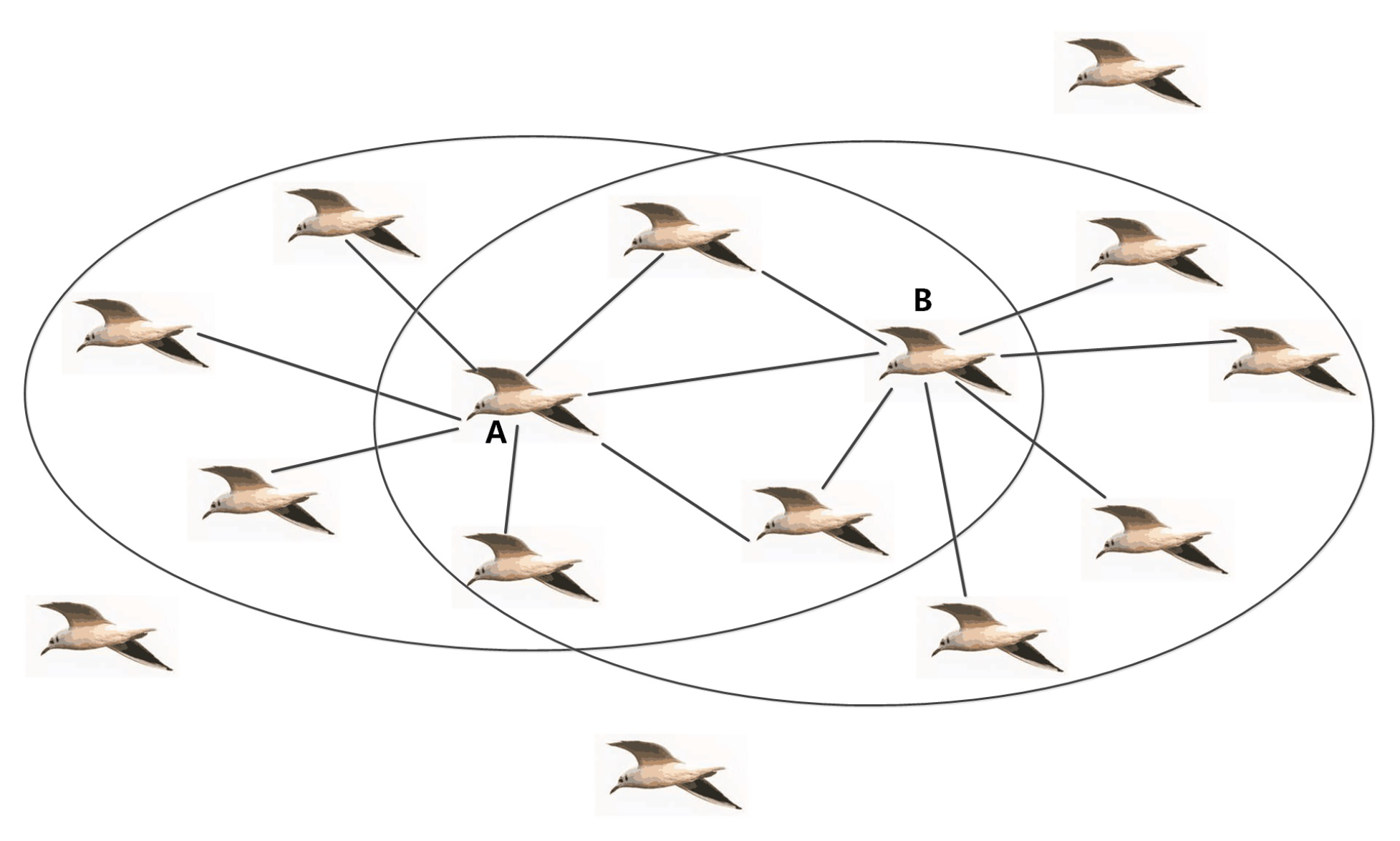
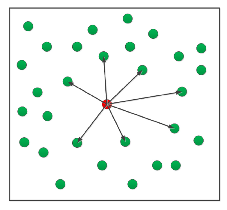
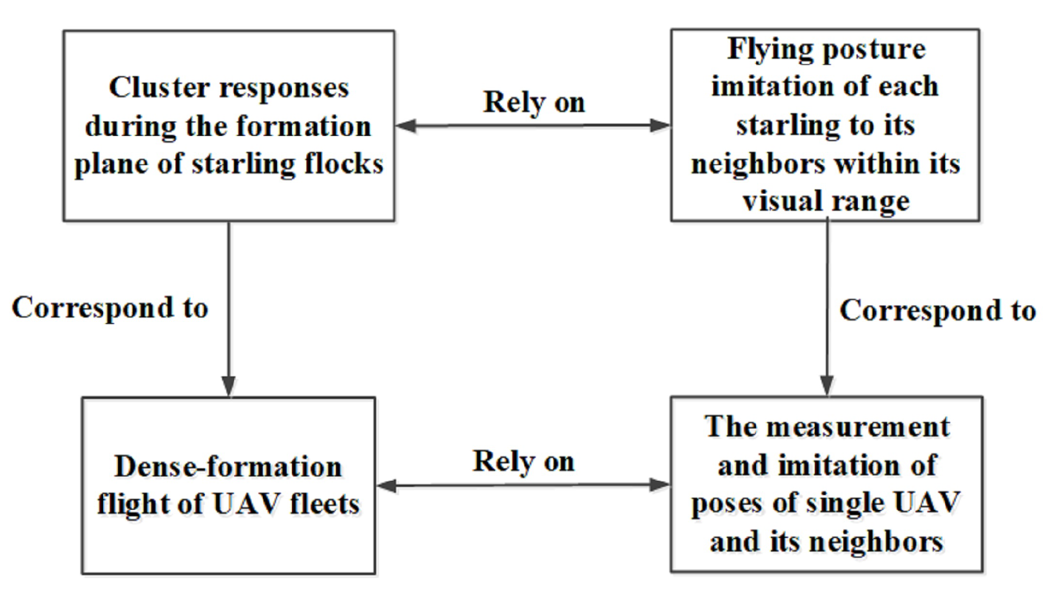
2.1. Characteristics of the Formation Mechanism of Starling Flocks

As the most widely distributed birds in the world, starlings are gregarious birds with strong imitation abilities. Thousands of starlings often fly together with a small distance between individuals, and their formations are complex and change frequently with frequent splitting and merging, enabling them to evade predators. Biologists and physicists found that, when a starling flock flies [50,51,52], there is a mutual reference between neighboring individuals, and each starling only interacts with the surrounding 6–7 individuals, as shown in Figure 1. In addition, scholars verified that the choice of reference neighbors is based on the topological model rather than the Euclidean geometric model, as shown in Figure 2 and Figure 3. The position of each bird, i, and its velocity were represented by $p_i$ and $V_i$, repetitively, and the dynamics model is

$$\overrightarrow{p_i}(t+1)=\overrightarrow{p_i}\left(t\right)+\overrightarrow{V_i}(t+1)$$

(1)

$$\overrightarrow{V_i}(t+1)=\frac{\left[{\theta }_i\left(t\right)+\sum _j{\theta }_j\left(t\right)\right]}{N_i+1}$$

(2)

where $N_i$ is the the total number of individuals that bird i can interact with.

In the Euclidean geometric model, bird i interacts with all neighboring individuals within a fixed distance $\overline{r}$, while in the topological model, bird i interacts with its $n_c$ neighboring individual, i.e., $N_i=n_c$. The specific mathematical model is as follows:

Let A = [$a_{ij}$] be the adjacency matrix among individuals; then, the Euclidean model is:

$$a_{ij}\left(t\right)=\left\{\begin{array}{cc}1\hfill & \mathrm{if}\left|\left|r_{ij}\left(t\right)\right|\right|\le \overline{r}\hfill \\ 0\hfill & \mathrm{if}\left|\left|r_{ij}\left(t\right)\right|\right|>\overline{r}\hfill \end{array}\right.$$

(3)

where $r_{ij}\left(t\right)$ is the distance from individual i to j, and $\overline{r}$ is the distance range established for communication.

Additionally, the topological mode is:

$$a_{ij}\left(t\right)=a_{ij}\left(t_0\right)\forall t\ge 0,\left|\left|r_{ij}\left(t\right)\right|\right|\in {\mathbf{R}}^{+}$$

(4)

where $a_{ij}\left(t_0\right)$ is the flag bit of the communication at the initialization time $a_{ij}$. $\left(t_0\right)=0$ indicates no communication connection, and $a_{ij}\left(t_0\right)\ne 0$ means such a connection exists.

Second, when the predator is moving in the opposite direction to the flock and there is a vertical offset d, the predator exerts a repulsive force on each bird, which attenuates as the bird moves further away from the predator. As shown by a large number of simulated numerical experiments, under different initial conditions, the clusters of two models present different grouping probabilities after being attacked by predators. Specifically, under the Euclidean model, the flock is usually dispersed into five groups, indicating low restoration capacity of the model. In contrast, it is highly possible for flocks to maintain a complete group under the topological model, and the original group is not easily dispersed, showing strong cohesion. Therefore, it is concluded that when flocks of starlings fly in nature, the choice of reference neighbors is not based on the Euclidean geometric model, but on the topological model [50].

When starlings fly in flocks, the plane direction of the entire formation is integrated. Specifically, the direction and speed of individual movements are initially haphazard, but through continued local interactions between individuals, they eventually fly in the same direction and speed as the movement of the entire flock. The $\Phi$-order parameter is generally used to characterize the synchronization index for the motion direction of all individuals in the starling cluster system. The formula is as follows:

$$\Phi =\parallel \frac{1}{N}\sum _{i=1}^n\frac{\overrightarrow{V_i}}{\parallel V_i\parallel }\parallel$$

(5)

where $V_i$ represents the speed of the ith starling, and N denotes the total number of the entire flock. The value of $\Phi$ will be zero if each starling flies in a different direction and speed; conversely, it will be close to one if most starlings fly in the same direction. Scholars analyzed 24 starling flocks and found that their flight direction has global orderliness [51]. When the perception is uncertain, interacting with the neighboring 6–7 starlings is an optimal choice to balance the cohesion of the flock and individual cost. The plane status of starling flocks can change correlatively: the plane state change of a single starling will affect all other individuals in the entire flock, regardless of the flock size.

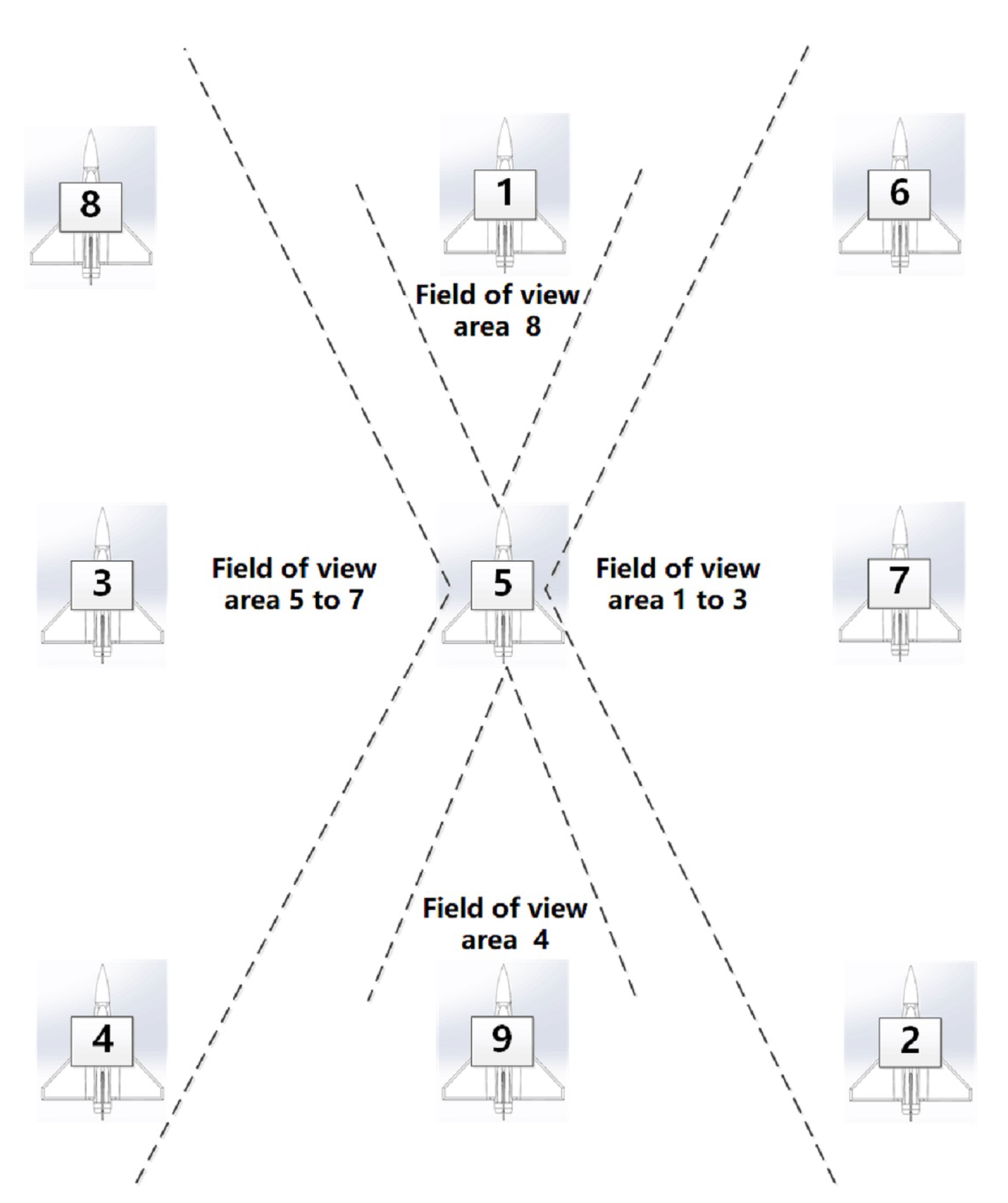
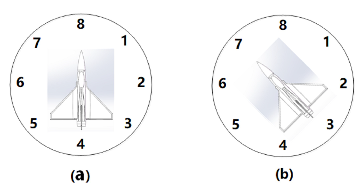
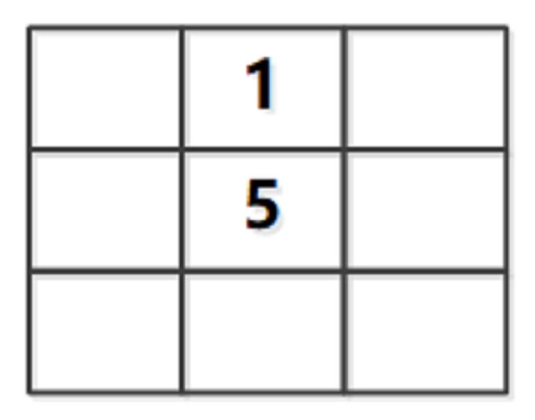
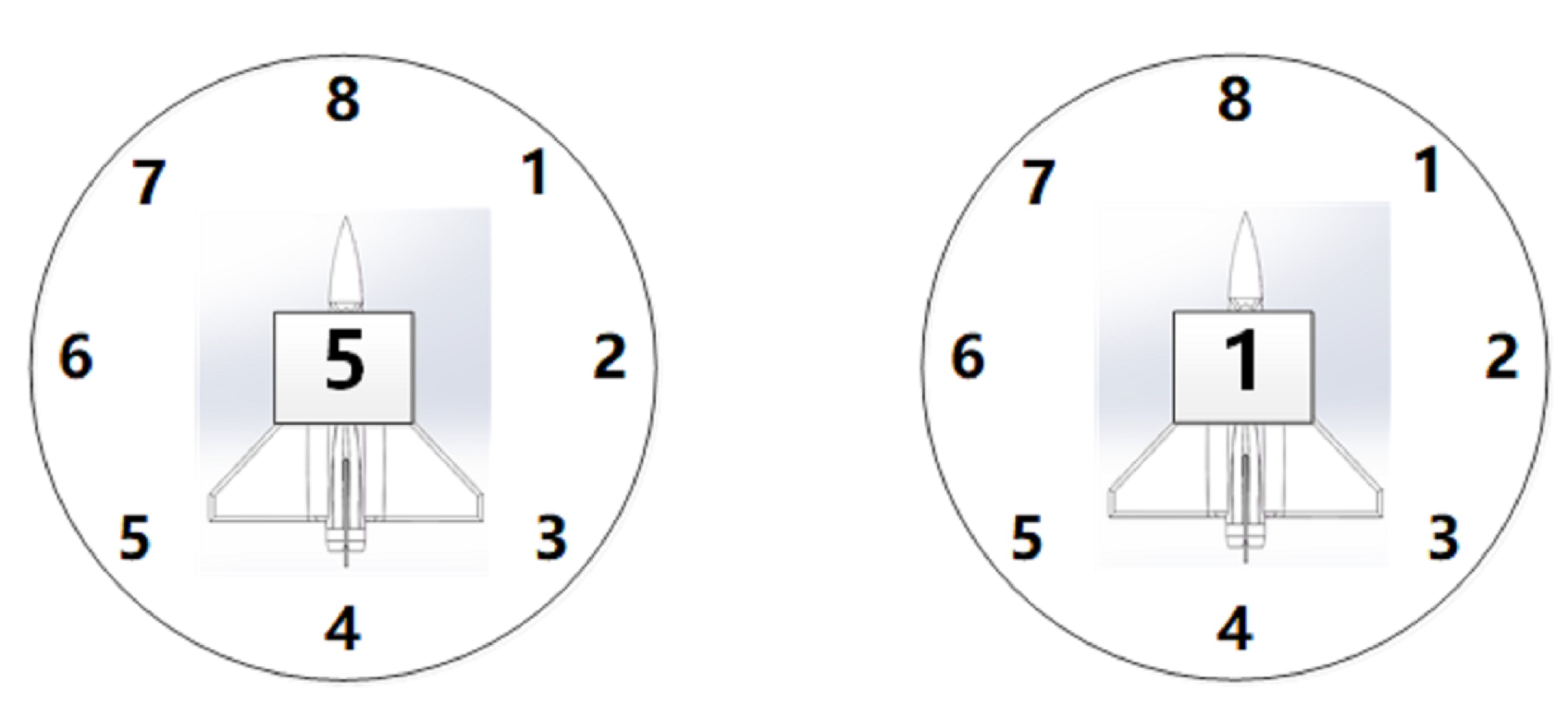
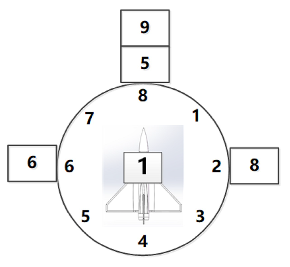
2.2. The Distribution of Visual Sensors and Cooperative Targets in UAVs Based on the Bionics of Starlings

As the whole plane formation system is based on the formation principle of starling flocks, each UAV in the fleet shall have a similar visual function as a single starling. The compared architecture between starling flocks and UAV fleets is shown in Figure 4:

To enable the UAV to observe the flying posture of its surrounding UAVs as starlings do, each UAV was equipped with visual sensors and high-precision ranging sensors on the left side, right side, directly behind and in front (these items of equipment are not necessarily on the directly above and below orientations because the plane formation was conducted on a single plane). For a more visual indication of the orientation, we give a top view of the FOV distribution of a 3 × 3 size UAV formation in Figure 5. As can be seen, there are eight basic directional positions (see details in Figure 6a) determined by the inertial navigation equipment. The flying postures on these positions can be observed by the two sensors equipped. For example, the UAVs numbered 1, 6, 7, 2, 9, 4, 3, and 8 locate the 8th, 1st, 2nd, 3rd, 4th, 5th, 6th, and 7th directions of the No.5 UAV, respectively.

These directions were fixed after the UAV joined the formation. No matter how the UAV turned during flying, the eight directions would always remain the initial state (as shown in Figure 6b), so that each UAV can obtain a fixed reference versus the surrounding UAVs. At the same time, the vision system of the UAV can collect the signal conditions of cooperative signal lamps located on the UAV surface in different directions (as shown in Figure 7), thus determining the flying posture of a referenced UAV in each direction. Each UAV can also collect the real-time flying distance between the referenced UAVs and itself together with the high-precision ranging sensors.

3. Formation Methods and Simulation

Based on the work above, this chapter elaborates the distributed formation method based on the 3 × 3 magic square and the chain rules of visual reference. Using the method, the advantages of the VM and its improved models are integrated into the large-scale UAV cluster formation, so that the VM’s redundant neighborhood information can be avoided in its formation. Notably, this method is characterized by a more stable neighborhood information collection than the RLosVM model and the memory function of the FOVM model. In addition, the dynamic visual reference in the FNN model has been improved to enhance the formation’s anti-jamming and anti-deception capacity.

First, the formation was divided into two areas, kept at a certain distance to be anti-jamming. One was the unformatted UAV area, and the other was the formatted area. The involved UAVs could fly freely in the first area and at a random position outside the formatted area. When entering the formatted area, UAVs have their designated routes until arriving at the terminal. However, the routes of all UAVs were constrained by the grid formation, in which each UAV in flight maintained a certain distance, the same altitude and the same speed between them, using airborne distance sensors and their vision system. Based on the 3 × 3 magic square and the chain rules of visual reference, the vision system determines which drones in which directional positions can be referenced to guide the formation.

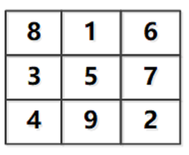
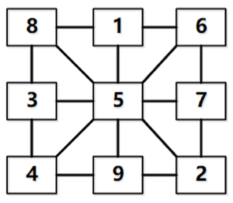
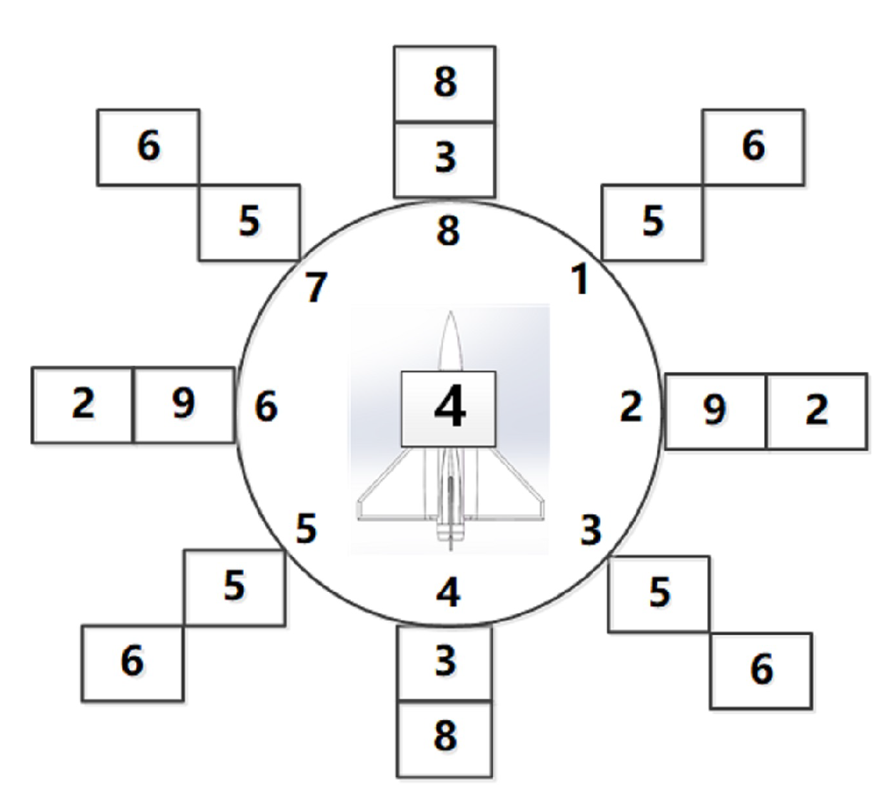
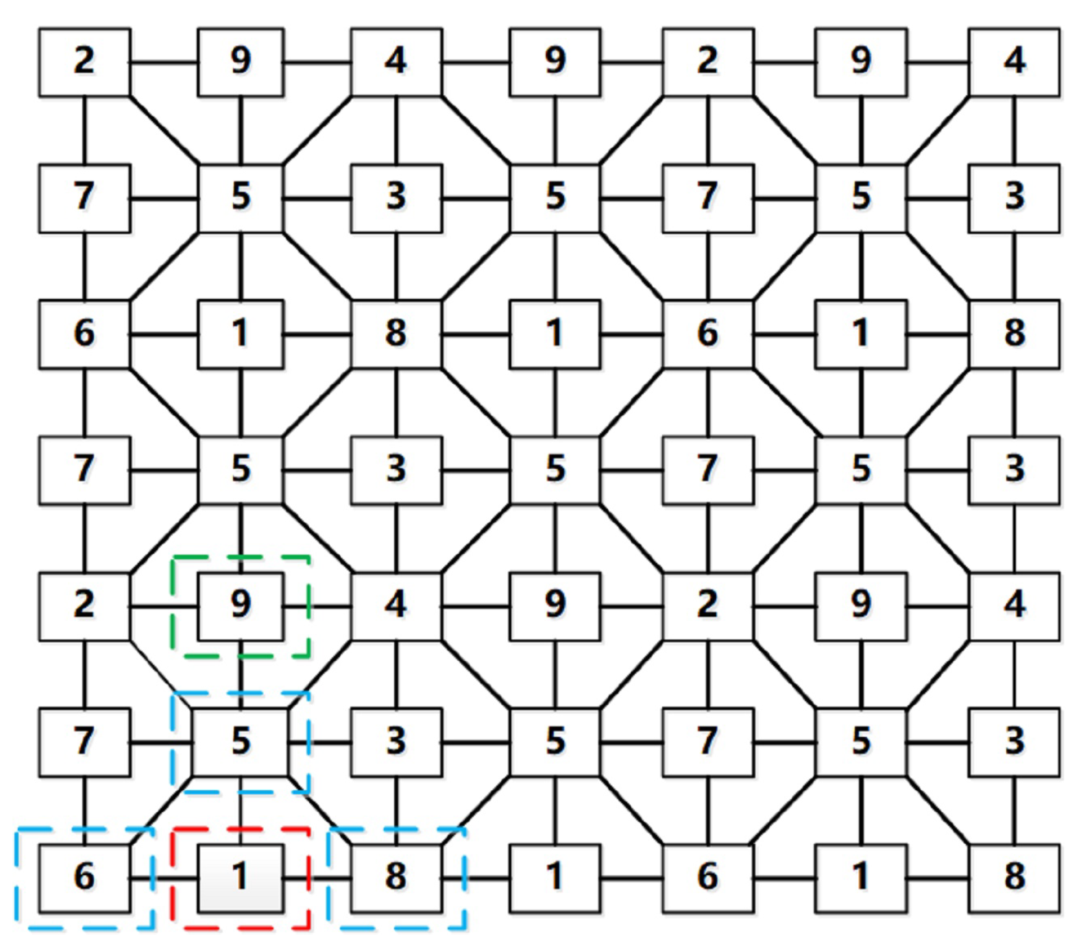
3.1. Distributed Formation Method Based on the 3 × 3 Magic Square and the Chain Rules of Visual Reference

For the formatted areas, a suppositional 3 × 3 magic square grid was set. The size of the square varied according to the scale of formation. Each square was marked with a number to show its position. For instance, Figure 8 is a typical 3 × 3 magic square diagram.

When the first UAV entered the formatted area, the very place it arrived was the square numbered 5, as shown in Figure 9. Afterward, the second UAV flew from the unformatted area to the square numbered 1.

As mentioned above, the visual sensor of each UAV could sense 8 basic directions in the same plane (Figure 6). Thus, the eight directions of UAVs in grids 5 and 1 are shown in Figure 10.

According to Figure 9 and Figure 10, the UAV in square 1 was in direction 8 of the UAV in square 5, whose airborne visual sensor identified the cooperation signal of the UAV in square 1. Thus, the poses of the UAV in square 1 could be obtained. The UAV in square 1 could offer reference to that in square 5 in direction 8. Similarly, the UAV in square 5 was in direction 4 of the UAV in square 1, whose airborne visual sensor identified the cooperation signal of the UAV in square 5. Therefore, the poses of the UAV in square 5 could be obtained. The UAV in square 5 was set as the reference for the UAV in square 1 in its direction 4. Similarly, through this visual cross-reference, UAVs could be formatted in other parts of the 3 × 3 magic square.

After the formation, a visual reference topological structure diagram of the 3 × 3 magic square was formed, as shown in Figure 11, where node numbers of the square referred to individual UAVs, and the lines between nodes showed the visual reference among UAVs.

According to the 3 × 3 magic square agreement and chain rules of visual reference, UAVs to be referred must meet two prerequisites. First, the numbers of UAVs and their reference must be in the same line in the topological structure diagram. Second, in the same line, there must be three nodes in that direction, with each of their numbers adding up to be 15. With these two prerequisites, UAVs at the nodes could be viewed as references. For instance, in Figure 11, UAVs at square 8 would refer to UAVs in square 1 and square 6 in direction 2, UAVs in square 5 and square 2 in direction 3, and UAVs in square 3 and square 4 in direction 4. In these three reference directions (2, 3, and 4), the sum of numbers in the three nodes was 15, satisfying the 3 × 3 magic square agreement and chain rules of visual reference. Thus, UAVs at square 8 could refer to squares 1, 6, 5, 2, 3, and 4. UAVs at square 3 could refer to squares 8, 4, 5, and 7. Similarly, we could get the reference for UAVs at other squares based on this principle. For example, 6 UAVs could be the reference for UAVs at squares 2, 4, 6, and 8, 8 for UAVs at square 5, and 4 for UAVs at square 1, 3, 7, and 9.

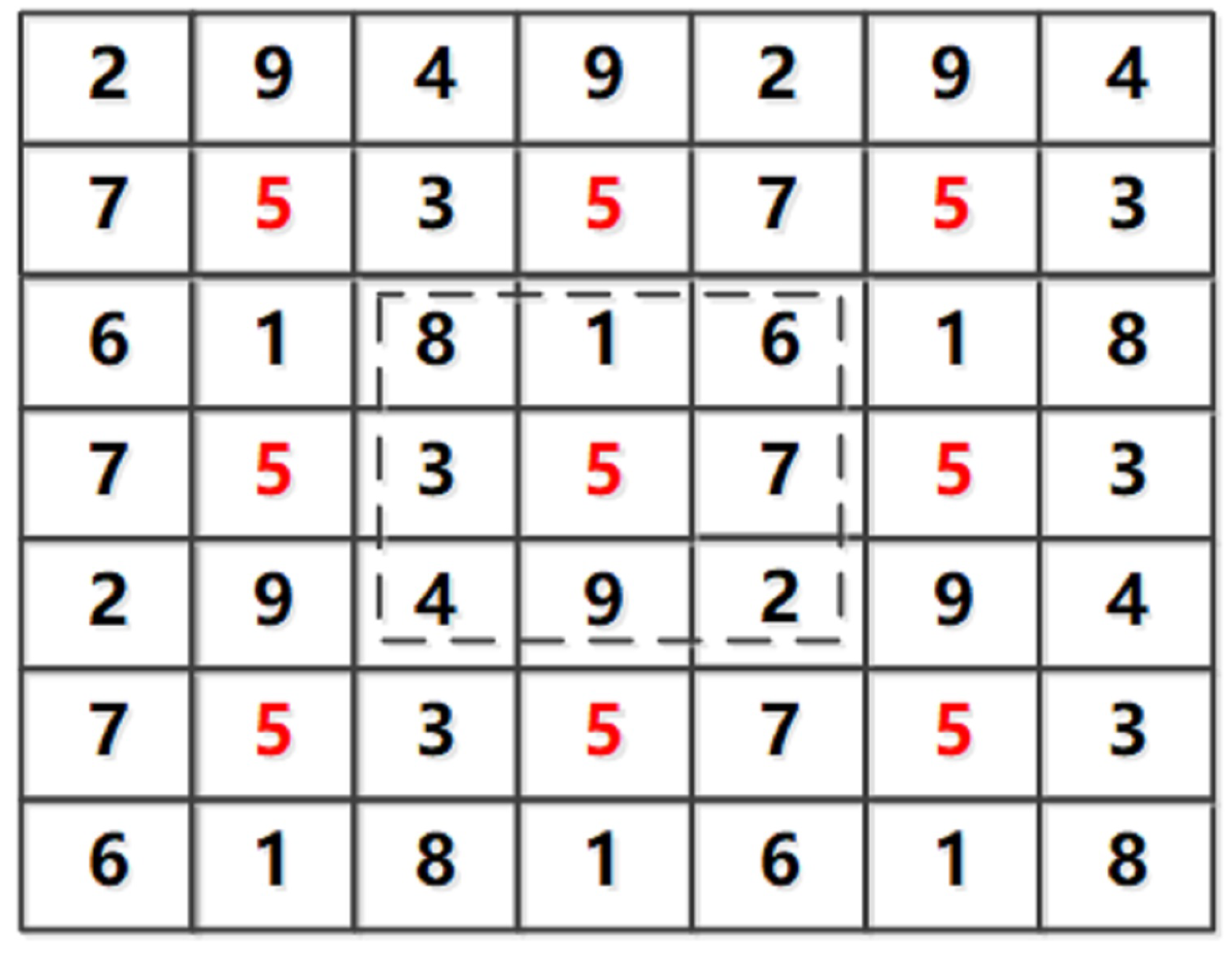
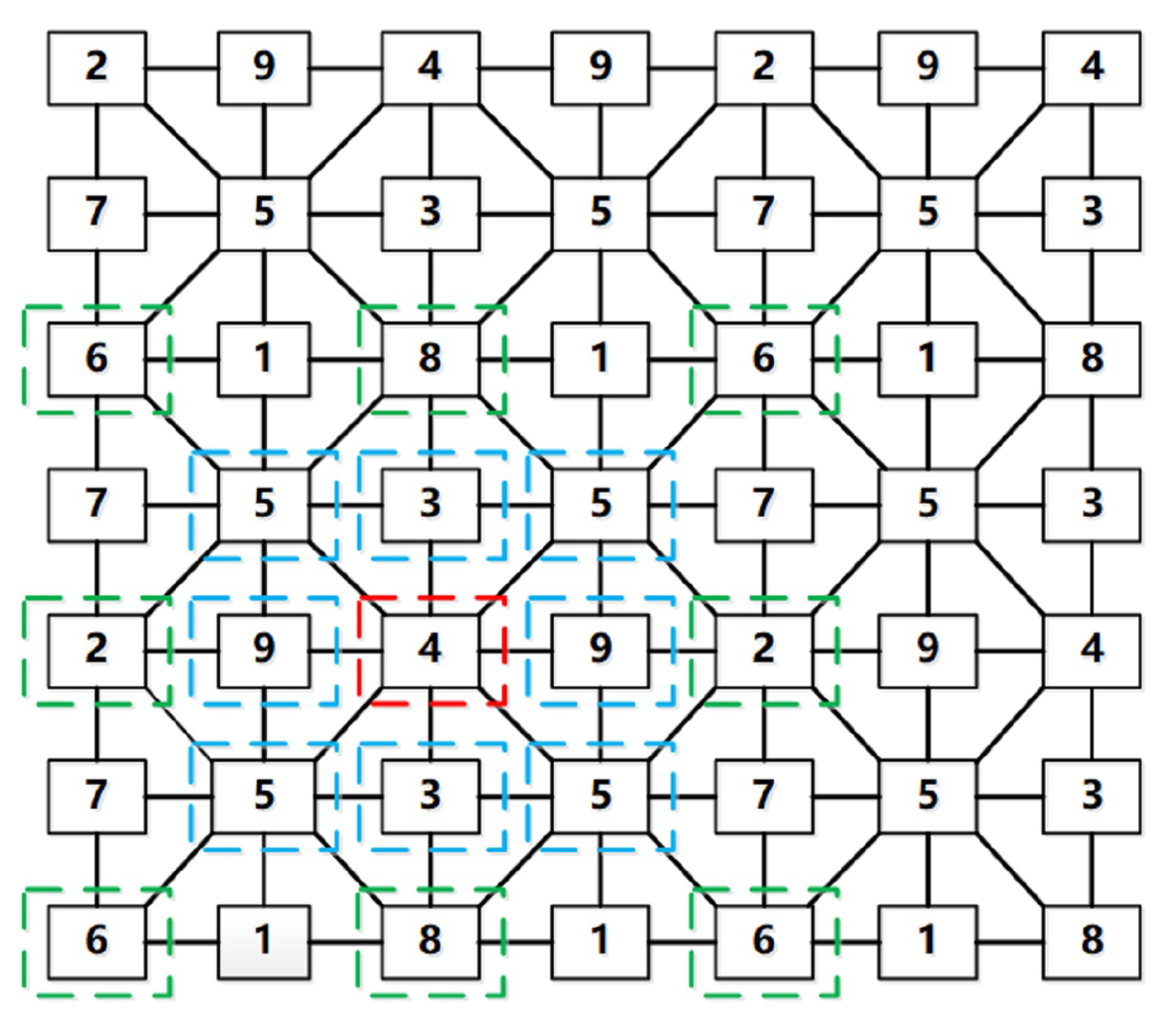
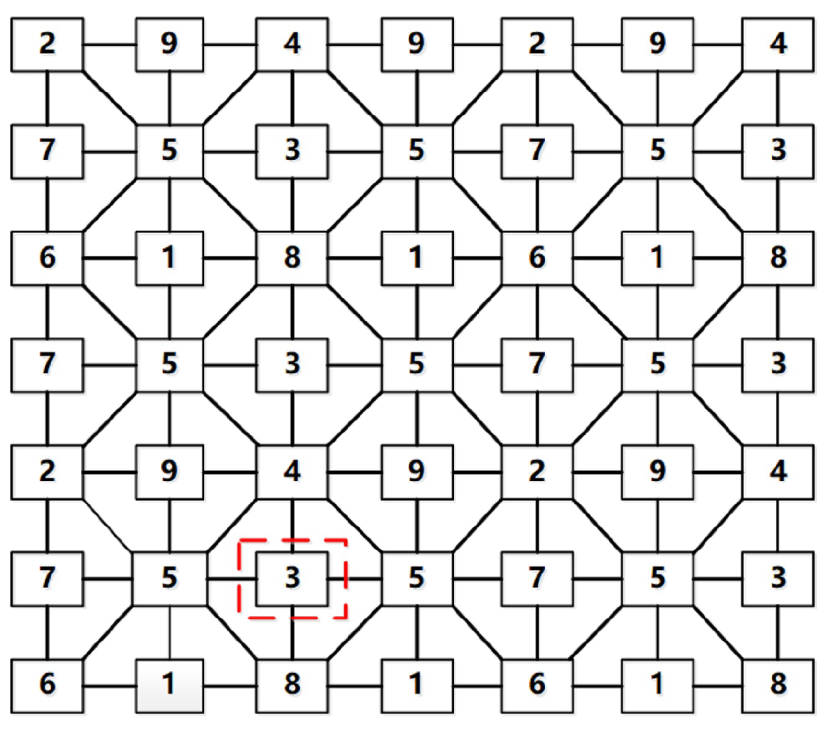
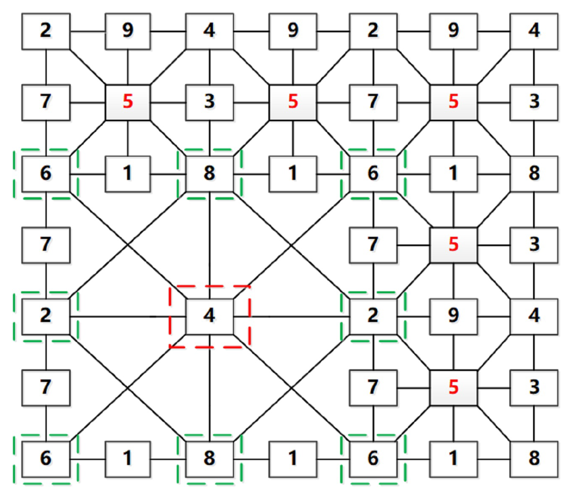
3.2. Visual Reference Topological Structure Diagram of the Nesting 3 × 3 Magic Squares

To expand the scale of the UAV formation, we expand the magic square by nesting under the exact mechanism of the first 3 × 3 magic square (circling the black dotted bordered rectangle in Figure 12). 3 × 3 magic squares were nested, forming a 7 × 7 magic square formation.

For the convenience of studying the formation of UAV clusters, the formation structure after each expansion should be in line with magic squares. For different scale square arrays, the grid numerical codes can be described by the following Equations (6) and (7):

$$n_5={(2n+1)}^2,(n=0,1,2,\dots )$$

(6)

$$M=[3+2(\sqrt{n_5}-1)]$$

(7)

where M refers to the number of clusters and $n_5$ refers to the number of 3 × 3 magic squares.

Based on the above formation mechanism and the above equations, we could achieve 11 × 11, 15 × 15, … expanded UAV formations. The expanded versions were more complex than the topologies of 3 × 3 magic squares, whose nesting structures made UAV formation more closely related, enhancing the formation stability. For instance, in the 7 × 7 visual reference topological structure diagram of UAV formation, UAVs at square 4 in the red dotted bordered rectangle (Figure 13) satisfied the 3 × 3 magic square agreement and the chain rules of visual reference, as shown in Figure 14. According to the 3 × 3 magic square agreement and chain rules of visual reference, the UAV at square 4 in the red-dotted bordered rectangle could refer to UAVs at squares 5, 9, 5, 3, 5, 9, 5, and 3 (as marked by the blue dashed box in Figure 13) in direction 1–8 as well as squares 6, 2, 6, 8, 6, 2, 6, and 8 (as marked by the green dashed box in Figure 13) in direction 1–8 of the extended nodes. In total, there are 16 UAVs in line with the prerequisites of UAVs for reference, as shown in Figure 14. If they were destroyed, the UAV at square 4 in the red dotted bordered rectangle would be out of the formation.

Similarly, for the UAV at square 1 (as marked by the red dashed box in Figure 15), 4 UVAs meeting the 3 × 3 magic square agreement and the chain rules of visual reference, as shown in Figure 16, respectively, were at neighboring squares 8, 6, and 5 (as marked by the blue dashed box in Figure 15) in direction 2, 6, and 8, as well as square 9 (as marked by the green dashed box in Figure 15) in direction 8 of the extended node. Without these 4 UAVs for reference, the UAV at square 1 will be out of formation. It could be seen that nodes with fewer reference UAVs were located at the margin of the formation. Such is the case of Figure 15, where the UAV at square 1 in the dotted bordered rectangle was in an individual 3 × 3 magic square without nested relation with others.

3.3. 11 × 11 Matlab Simulations of UAVs Magic Square Formation

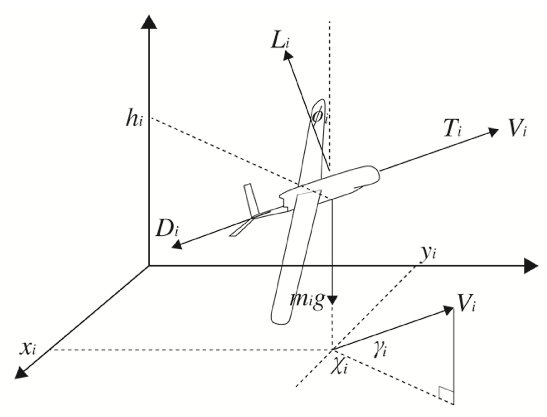
3.3.1. UAV Model

In real UAVs with different model parameters, there are multiple aerodynamic configurations, causing the variance of mathematical modeling. To simplify the algorithm of upper control, we suppose that the UAV internal-loop is controlled by autopilot. Thus, the model could be built with the UAV position and velocity external-loop model as the upper control algorithm, as shown in Figure 17.

The mathematical model of the $UA{V}_i$ is expressed as Equation (8)

$$\left\{\begin{array}{c}\dot{x_i}=V_{i}cos{\gamma }_{i}cos{\chi }_i\hfill \\ \dot{y_i}=V_{i}cos{\gamma }_{i}sin{\chi }_i\hfill \\ \dot{h_i}=Vsin{\gamma }_i\hfill \\ \dot{V_i}=\frac{T_i-D_i}{m_i}-gsin{\gamma }_i\hfill \\ \dot{{\gamma }_i}=\frac{Lcos{\Phi }_i-m_{i}gcos{\gamma }_i}{m_i{V}_i}\hfill \\ \dot{{\chi }_i}=\frac{L_{i}sin{\Phi }_i}{m_i{V}_{i}cos{\gamma }_i}\hfill \end{array}\right.$$

(8)

where $i=1,\cdots ,N$. $x_i,y_i,$ and $h_i$ correspond to the down-range, cross-range, and altitude displacement. $V_i$ refers to the airspeed of $UA{V}_i$, ${\gamma }_i$ is the plane path angle, and ${\chi }_i$ represents the heading angle. $T_i$ is the engine thrust, $D_i$ refers to drag, $m_i$ is the quality of $UA{V}_i$, and g represents the gravity acceleration. Furthermore, $L_i$ refers to lift, and ${\Phi }_i$ is the bank angle.

Equation (9) can be achieved with the transformation of the mathematical model.

$$\left\{\begin{array}{c}\ddot{x_i}=u_{xi}\hfill \\ \ddot{y_i}=u_{yi}\hfill \\ \ddot{z_i}=u_{hi}\hfill \end{array}\right.$$

(9)

$u_{xi}$, $u_{yi}$, and $u_{hi}$ are the subjunctive control input, and the transformation relationship between the executive order and subjunctive control input can be expressed as Equation (10),

$$\left\{\begin{array}{c}{\Phi }_i=arctan\left(\frac{u_{yi}cos{\chi }_i-u_{xi}sin{\chi }_i}{(u_{hi}+g)cos{\gamma }_i-(u_{xi}cos{\chi }_i+u_{yi}sin{\chi }_i)sin{\gamma }_i}\right)\hfill \\ L_i=m_i\frac{(u_{hi}+g)cos{\gamma }_i-(u_{xi}cos{\chi }_i+u_{yi}sin{\chi }_i)sin{\gamma }_i}{cos{\Phi }_i}\hfill \\ T_i=m_i[(u_{hi}+g)sin{\gamma }_i+(u_{xi}cos{\chi }_i+u_{yi}sin{\chi }_i)cos{\gamma }_i]+D_i\hfill \end{array}\right.$$

(10)

where tan(${\chi }_i$) = $\dot{y_i}$/$\dot{x_i}$, and $sin\left({\gamma }_i\right)=\dot{h_i}/V_i$. Therefore, the subjunctive control input is designed as Equation (9), and the real input of the UVA could be calculated through Equation (10), which can be expressed as the state place:

$$\left\{\begin{array}{c}\dot{z_i}=A{z}_i+B{u}_i\hfill \\ p_i=C_p{z}_i\hfill \\ v_i=C_v{z}_i\hfill \end{array}\right.$$

(11)

where $z_i={[{p_i}^T,v_i]}^T$, $p_i$ refers to the position vector, $v_i$ is the speed vector, and $u_i={[u_{xi}^T,u_{yi}^T,u_{hi}^T]}^T$ shows the subjunctive control input.

$$A_i=\left[\begin{array}{cc}0& 1\\ 0& 0\end{array}\right] \otimes I_3,B_i=\left[\begin{array}{c}0\\ 1\end{array}\right] \otimes I_3,C_p=\left[\begin{array}{cc}1& 0\end{array}\right] \otimes I_3,C_v=\left[\begin{array}{cc}0& 1\end{array}\right] \otimes I_3$$

(12)

$I_3\in R^{3\times 3}$ refers to the identity matrix, and ⊗ is the Kronecker product.

In Equation (10), the air resistance $D_i$ can be expressed as Equation (13).

$$D_i=0.5\rho {(V_i-V_{wi})}^{2}S{C}_{D0}+\frac{2k_d{k}_n^2{L}^2}{\rho {(V_i-V_{wi})}^{2}S{g}^2}$$

(13)

where $\rho$ refers to the air density, $C_{D0}$ represents the zero-lift drag coefficient, $V_{wi}$ refers to gust, S is the wing area, $k_d$ is the induced drag, and $k_n$ refers to the load-factor effectiveness.

The mathematical modeling of gust can be expressed as Equation (14).

$$\left\{\begin{array}{c}{V}_{wi}={\overline{V}}_{wi}+\delta V_{wi}\hfill \\ {\overline{V}}_{wi}=0.215V_m{log}_{10}\left(h_i\right)+0.285V_m\hfill \end{array}\right.$$

(14)

where ${\overline{V}}_{wi}$ is normal wind shear, $V_m$ refers to the mean wind speed and $\delta V_{wi}$ is the wind gust turbulence. The zero mean equals 0, and the standard deviation was 0.9$V_m$ for this Gaussian random variable.

3.3.2. Design of UAV Controller

Through an algorithm based on the 3 × 3 magic square grid, which was illustrated in Section 3, the expected position $p_{di}$ and expected speed of every $UA{V}_i$ could be calculated. Thus, the controller form of individual UAVs can be expressed as Equation (15).

$$u_i=k_p(p_{di}-p_i)+k_d(q_{di}-q_i)$$

(15)

where $k_p>0$ and $k_d>0$ are parameters of UAV PID controllers.

The values of each item in simulations are as shown in

Table 1. Settings of UAV Parameters.

Symbol	Value	Unit
$m_i$	20	kg
g	9.81	kg/m${}^2$
$\rho$	1.225	kg/m${}^3$
S	1.37	m${}^2$
$C_{D0}$	0.02	Non-dimensional
$k_d$	0.1	Non-dimensional
$k_n$	1	Non-dimensional
$V_m$	4	m/s (at $h_i=80$ m)
$T_i$	$[0,125)$	N
$L_i$	$(-294.3,392.4)$	N
${\Phi }_i$	$[-80,80]$	N
${\chi }_i$	$[-180,180]$	deg
${\gamma }_i$	$[-90,90]$	deg

.

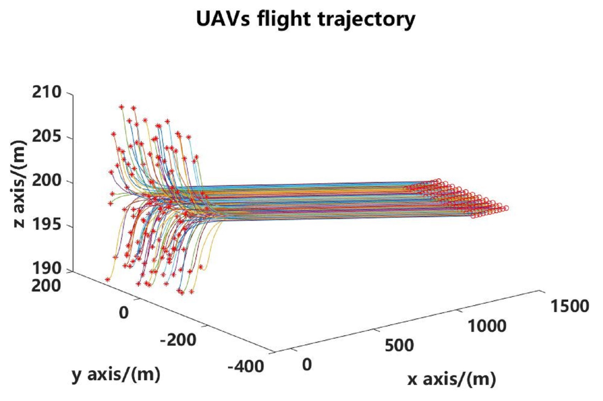
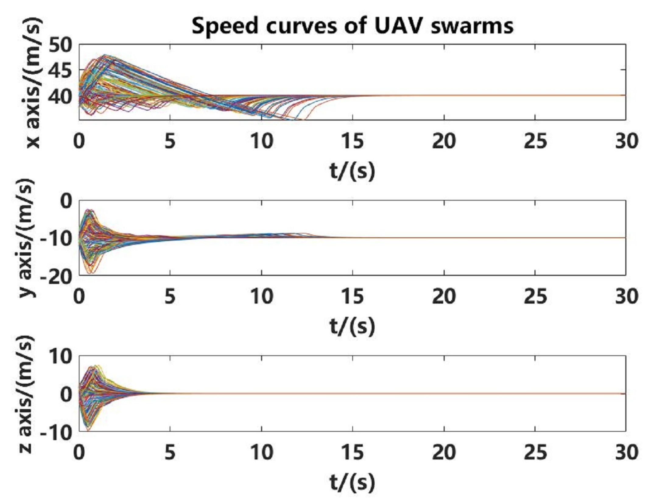
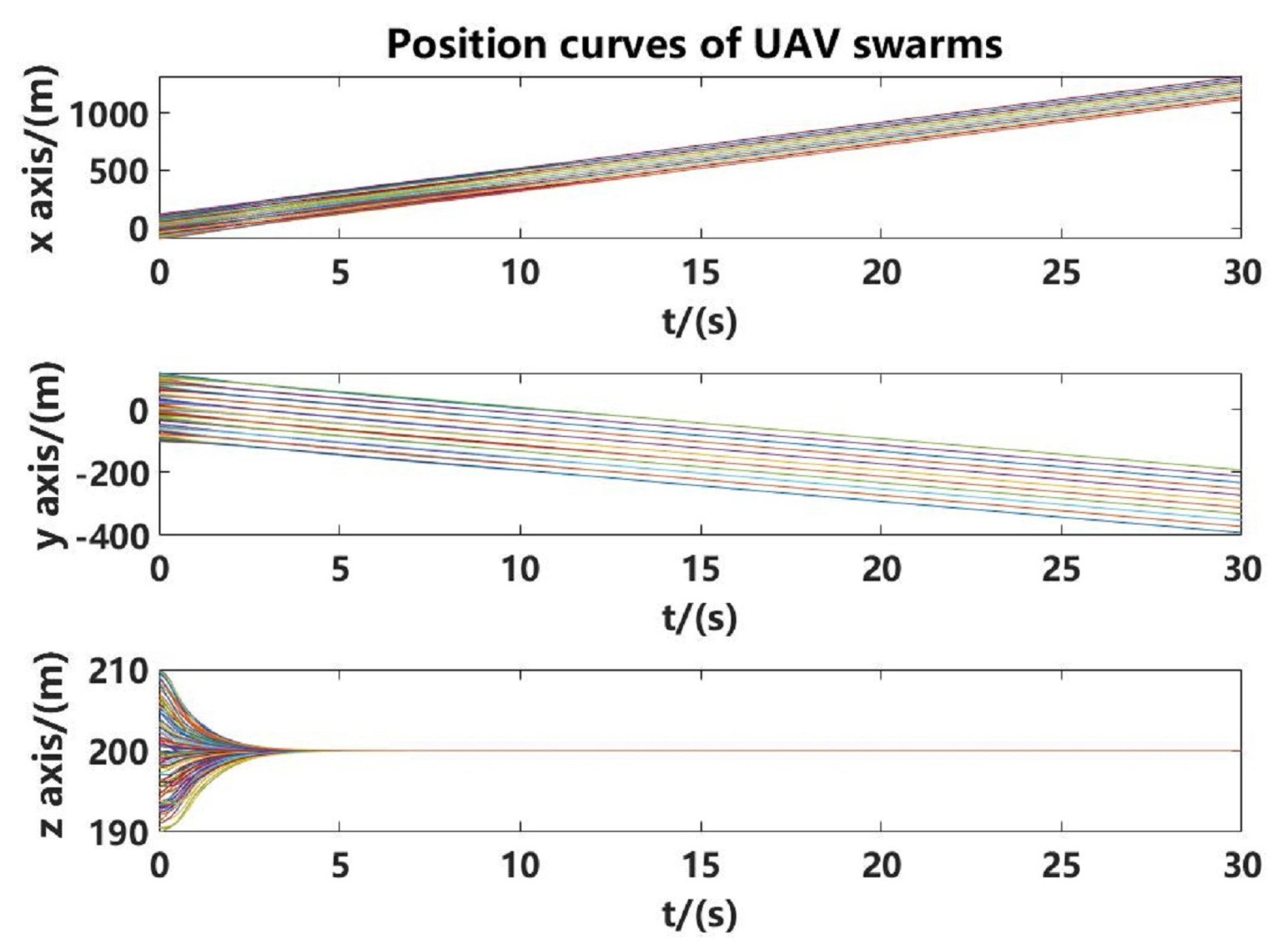
3.3.3. Simulations of Scale UAV Grid Formations

Considering different scales of nested magic squares, this study will not illustrate them one by one. However, they share the same formation rule and topological structure, so the 11 × 11-scale UAV grid formation (121 UAVs) was used as an example. Its simulation results are as shown in Figure 18, Figure 19 and Figure 20.

According to the UAV flying trajectory in the simulation results, it could be concluded that the UAV cluster initially moved from the unformatted sector to the formatted one. In addition, the initial flying orientation was along the x axis. From the curve graph, the cluster converged to 200 m in height within 5 s and soon entered the formatted sector. Based on the speed graph, all UAVs achieved uniform convergence in axis x, y, and z at 15 s, when the curve graph of controller output, controller input, and executive output achieved convergence. Thus, it can be seen that the 121 UAVs in that formation generally realized convergence in speed and completed the formation in 15 s. This formation is large in scale, stable in plane, and swift in convergence compared with other formations.

4. An Analysis on the Stability of the Visual Reference Topological Structure

In this chapter, the network connectivity index of graph theory was introduced to analyze the static stability of the visual reference topological structure of the nested magic squares. Meanwhile, a detailed description of the self-healing dynamic visual reference grid of UAV formations will be given based on the principle and argument mentioned in this study.

In this analysis, only nodes with close relations would be taken into account. For instance, in Figure 21, the UAV at square 3 in the red-dotted bordered rectangle could only refer to the UAVs at squares 4, 5, 8, and 5 in directions 8, 2, 4, and 6, respectively. If these nodes were destroyed, the UAV at square 3 would be out of the topology.

In this analysis, its basic concepts include network connectiveness, network resistance to destruction, network cutpoint, network vertex cutpoint, minimum vertex cutpoint, vertex impact, network impact, and network connectivity. Their specific definitions are given as follows:

Definition 1

(network connectiveness). In the network G(V,E), if there is a path from vertex v to v’, the two vertexes are connected. If for every pair of vertexes ($v_i$,$v_j$∈ V) in the network G(V,E), $v_i$ and $v_j$ are connected, then G is connected.

Definition 2

(network resistance to destruction). Several vertexes or chains should be destroyed to impede the connectivity of certain vertexes. The cohesion strength and connectivity degree are often used to show the resistance to destruction.

Definition 3

(network cutpoint). In the network G(V,E), if, for vertex v, its connected lines are deleted, the connected component of the network will be divided into two or more connected components. The vertex v will be called a cutpoint of G.

Definition 4

(network vertex cutpoint). In the network G(V,E), suppose V’⊆V; if G-V’ are disconnected, V’ will be called G’s cutpoint or vertex cutpoint. The vertex cutpoint with k vertexes will be called the k vertex cutpoint.

Definition 5

(minimum vertex cutpoint). In the network G(V,E), the vertex with the least points is called G’s minimum vertex cutpoint.

Definition 6

(vertex impact). In the network G(V,E), suppose that $d_i$ (i = 1,2,⋯, n). For the degrees of vertex $v_i$, the vector L = ($\frac{1}{d_1}$,$\frac{1}{d_2}$; then, ⋯,$\frac{1}{d_n}$) is called the vertex impact, showing the influence of vertexes on adjacent ones.

Definition 7

(network impact). In the network G(V,E), suppose A is the adjacent matrix of network G, and D is the vector showing the impact degree between adjacent vertexes. The network impact can be expressed as P = D·A, which indicates the influence of other vertexes on the network G.

Definition 8

(network connectivity). G(V,E) is an n-order connected network. If vertex cutpoints exist at G, the point of G’s minimum vertex cutpoint is called its connectivity. Otherwise, n − 1 will be its connectivity. In other words, the sub-graph is still connected after k − 1 vertexes are eliminated in a network with n vertexes (1 ≤ k ≤ n − 1). However, when k vertexes are removed, the graph will be disconnected or become a trivial graph. In this way, k refers to the connectivity of G, expressed as k(G) = k.

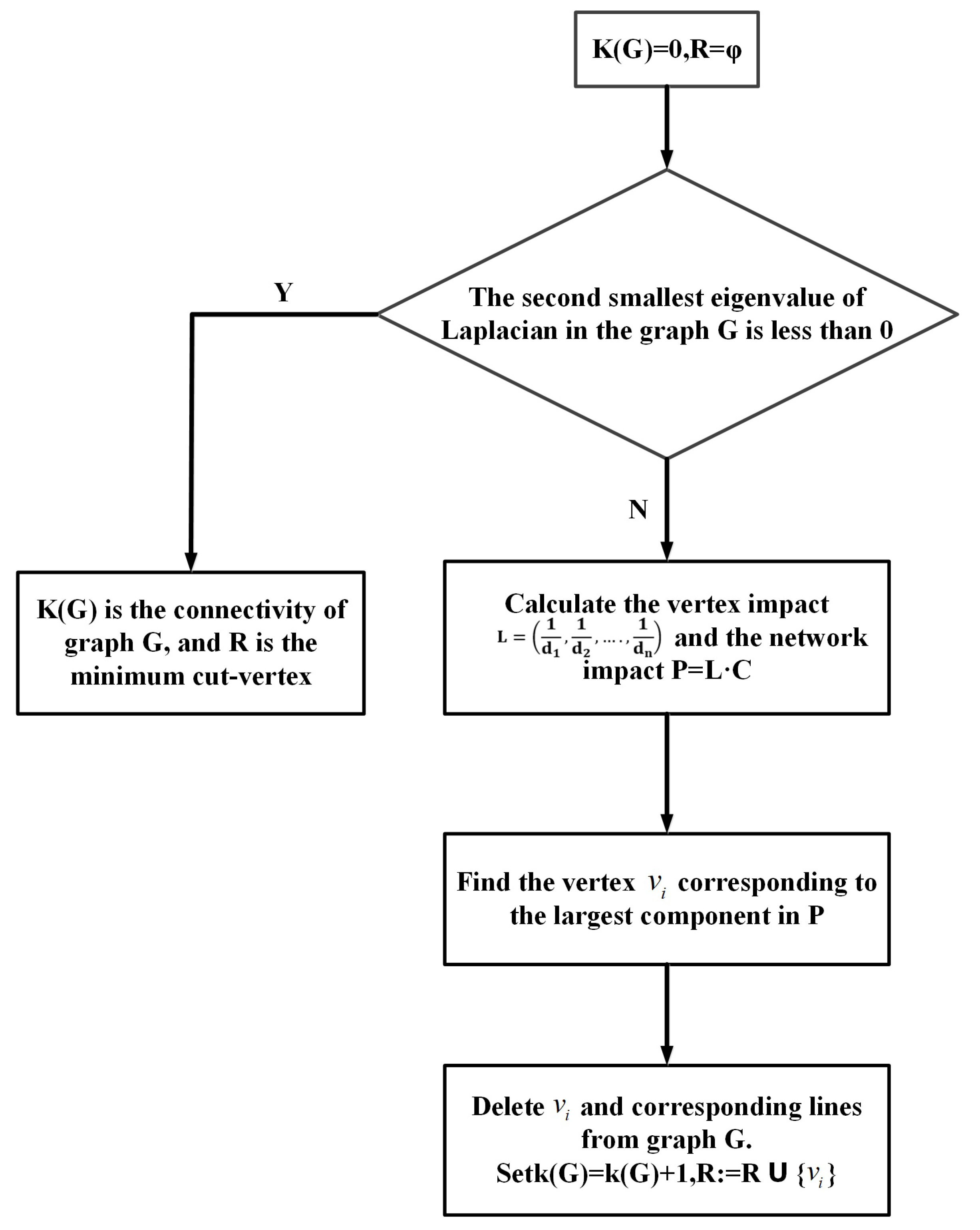
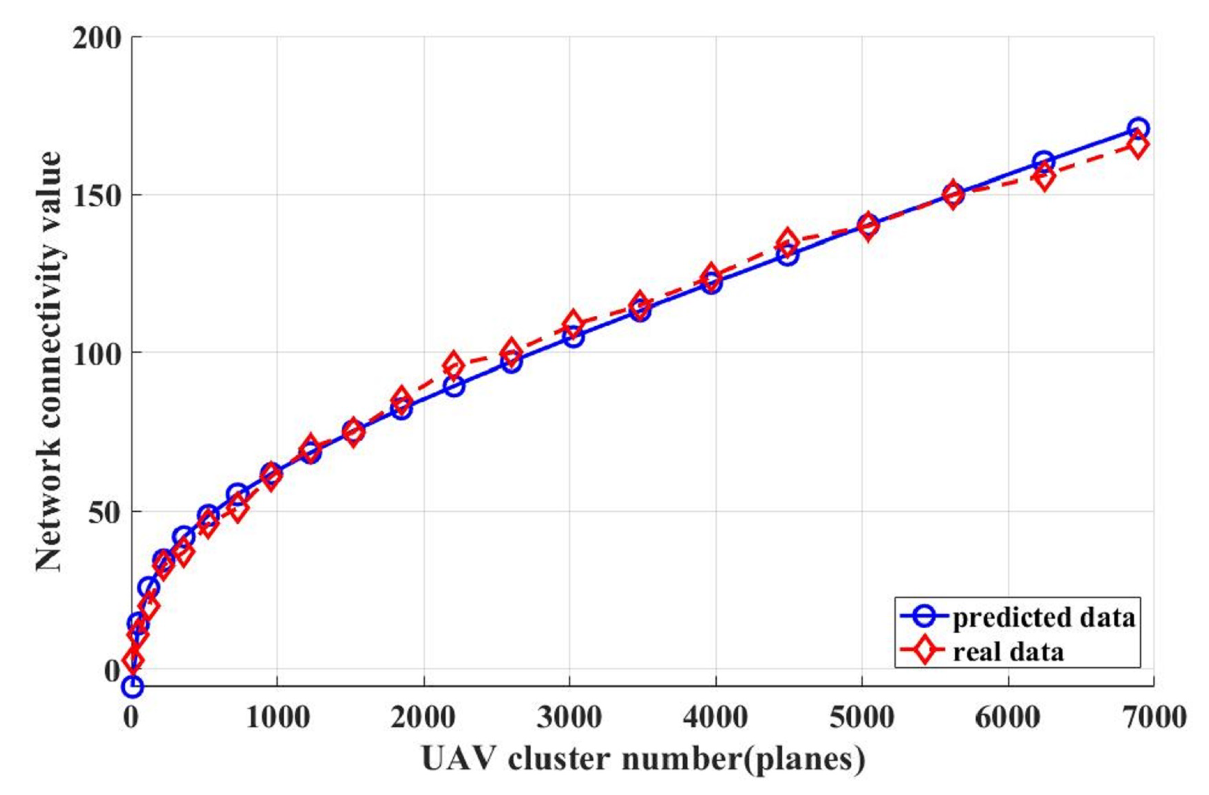
4.1. Calculation of Network Connectivity in the Undirected Topological Diagram

To calculate the network connectivity of the visual topological diagram for different scale UAV clusters, we adopted the algorithm mentioned in the Reference [53], which is more straightforward than the traditional algorithm. The flow chart of the algorithm is as shown in Figure 22. Condition: Suppose that G has n vertexes $v_i$ (i = 1, 2, ⋯, n); then, the adjacent matrix is C = ${\left(c_{ij}\right)}_{n\times n}$. If $v_i$ and $v_j$ are adjacent, $c_{ij}$ = 1. Otherwise, $c_{ij}$ = 0. Here, $d_i$ refers to the degree of the vertex $v_i$.

4.2. Matlab Simulations of Network Connectivity of Nested Magic Squares’ Topological Structure under Different-Scale UAV Formations

This chapter employed the matlab simulation of the network connectivity of the topological structure from 3 × 3 to 83 × 83 nested magic squares formation according to the connectivity algorithm. The regression curve equation of the connectivity was concluded, as shown in

Table 2. Network connectivity values of different-scale UAV formations.

UAV Cluster Number	Network Connectivity Value
9	3
49	11
121	20
225	33
361	37
529	46
729	51
961	61
1225	70
1521	75
1849	85
2209	96
2601	100
3025	109
3481	115
3969	124
4489	135
5041	140
5625	150
6241	156
6889	166

, and Figure 23.

This study used the least square method to establish the regression model curve via the network values of different-scale network topological diagrams, as shown in Figure 23. Thus, the network connectivity values of topological structures of any scale nested magic squares can be calculated.The regression model curve equation is:

$$K\left(G\right)=-30.7292-0.0146\left(M_n\right)+26.3306{log}_{10}\left(M_n\right)$$

(16)

where K(G) represents the network connectivity index and $M_n$ refers to the UAV cluster number.

According to the simulation results, the 95% confidence intervals of the gradients were [0.0131, 0.0161] and [21.9585, 30.7027], and the 95% confidence interval of the intercepts was [−41.4515, −20.0070]. The intercepts and gradients of the regression model curve equation satisfied the requirement. The network connectivity index of the visual reference topological diagram had an R2 variance-explained rate of 0.9937, proving the significance test of the regression equation with excellent fitting.

According to the fitted curve equation, the cluster accelerated in expanding, but the network connectivity increased rather slowly. However, the network connectivity is an index to evaluate the trivial graph formed after deleting k nodes in the network topological diagram. Thus, applying nested magic squares’ network topological diagrams into large-scale formations could help to greatly enhance the stability of UAV formations. The simulation results show that, at a formation size of 961 UAVs, the resulting visual reference network topology subgraph is still connected after the loss of a random 60 UAVs.

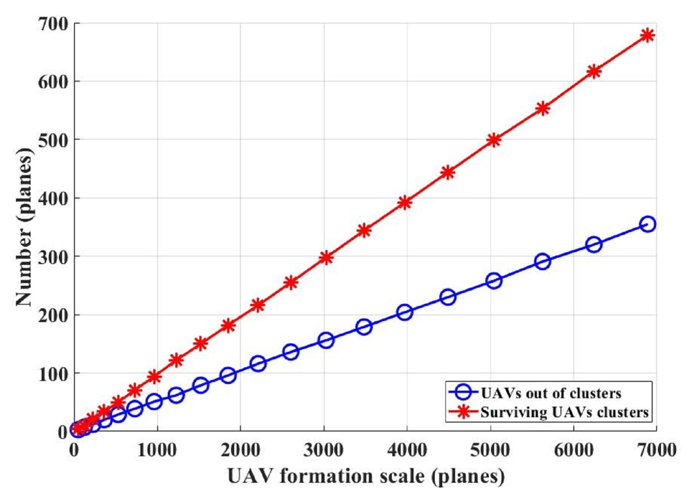
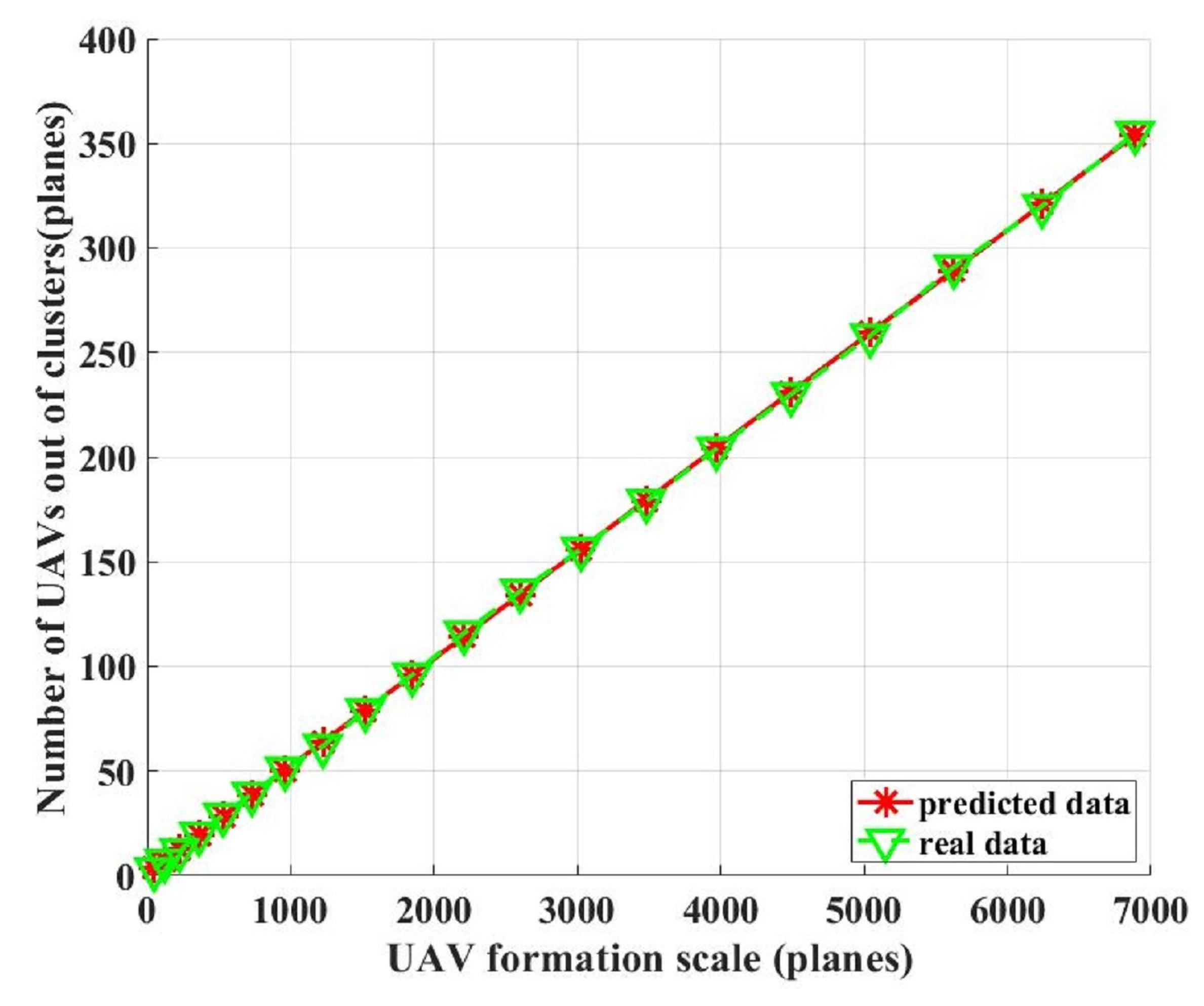
4.3. Dynamic Self-Healing of Grid Formation Based on the 3 × 3 Magic Square and the Chain Rules of Visual Reference

We calculated the network connectivity and concluded that the topological structure of nested magic squares has relatively high static stability. Still, the formation based on the 3 × 3 magic square and the chain rules of visual reference could lead to better stability. For instance, the UAV at square 4 in the dotted rectangle in Figure 13 has 16 planes that satisfy the reference principle, as shown in Figure 14. If the adjacent UAVs at squares 5, 9, 5, 3, 5, 9, 5, and 3 (UAVs in the blue dashed box) in directions 1–8 were destroyed due to fire attacks, the UAV at square 4 could seek reference from 8 UAVs (UAVs in the green dashed box) in its periphery. In this way, the formation could be maintained, and the regenerated topological structure diagram is shown in Figure 24. The general visual reference topology graph changes, but the UAV at square 4 in the dotted rectangle will be kept in the formation. Therefore, the formation based on the 3 × 3 magic square and the chain rules of visual reference not only has great stability but enjoys dynamic self-healing ability.

5. Simulations and Analysis in Battlefields

5.1. The Procedure of Matlab Simulations of UAV Formations in Battlefields

To evaluate the survival rate of a formation based on the 3 × 3 magic square and the chain rules of visual reference in battlefields, we used matlab to simulate the attacks on UAV formation in battlefields. There are six premises of the simulation experiments. First, different-scale UAV clusters will enter the enemy region and will be attacked after the formation. Second, once the grid formation is completed, all UAVs’ plane height, speed, and relative distance will remain unchanged until they reach the destination. Third, each fire attack on UAVs has a random aim and is completed once it is exerted. The number of UAVs to be destroyed can be set before simulation. Fourth, UAVs out of the formation are those which lose all reference planes in the grid formation. Fifth, surviving UAVs are those which are not destroyed and for which there is at least one reference UAV. Sixth, the UAV clusters will not defend or dodge, so the stability of the formation in worst-case scenarios can be obtained. Figure 25 is the flow chart of the detailed simulation.

Although the number of drones set to be destroyed is the same, there will be some variation in the number of drones out of formation as the aimed destructed areas were randomly set. For this reason, the simulation experiments were conducted 100 times with the same fight loss for the same-scale formation to obtain the average values of the UAVs which were out of formation and those which survived. Next, this study simulated the 3 × 3 to 83 × 83 grid formations and calculated the number of UAVs out of formation and surviving UAVs at 85% fight loss.

5.2. The Procedure of Matlab Simulations of UAV Formations in Battlefields

To test and verify the survival rate of formations with nested magic square topological structures based on the 3 × 3 magic square and the chain rules of visual reference in battlefields, we adopted matlab simulations to obtain the regression curve of UAVs out of the formation and surviving UAVs in different-scale formations with the fight loss set at 85%. These values can be expressed in the following equation:

$$H_n=M_n-D_n-I{s}_o$$

(17)

where $H_n$ is the remaining UAVs, $M_n$ refers to the UAVs before entering the battlefield, $D_n$ represents the total destructed UAVs, and $I{s}_o$ stands for the undestroyed UAVs that get out of formation.

The simulation results are as shown in

Table 3. Simulation results of UAV formations with 85% fight loss.

UAV Formation Scale (Planes)	UAVs Out of Clusters (Planes)	Surviving UAV Clusters (Planes)
49	3	4
121	7	10
225	12	21
361	20	34
529	29	50
729	39	71
961	51	94
1225	62	122
1521	79	150
1849	96	182
2209	116	216
2601	136	255
3025	156	298
3481	179	344
3969	204	392
4489	230	444
5041	258	499
5625	291	553
6241	320	617
6889	355	679

and Figure 26.

The least square method was adopted to make the curve fitting simulations of UAVs out of clusters and surviving UAVs clusters with 85% fight loss, and the results are as shown in Figure 27 and Figure 28.

The regression model equation of UAVs out of clusters can be expressed as:

$$R_a=0.0512M_n+1.1267$$

(18)

where $R_a$ is the number of UAVs out of clusters, and $M_n$ refers to the number of clusters.

According to the simulation results, the 95% confidence interval of gradients in the curve model was [0.0510, 0.0515], and that of intercepts was [0.3620, 1.8914], so the intercepts and gradients of the regression model curve equation satisfied the requirement. The R2 variance explained rate was 0.9999, proving the significance test of the regression equation with excellent fitting.

The regression model equation of UAVs out of clusters can be expressed as:

$$R_b=0.0989M_n-1.1704$$

(19)

$R_b$ is the number of surviving UAVs, and $M_n$ refers to the number of clusters.

According to the simulation results, the 95% confidence interval of gradients in the curve model was [0.0987, 0.0992], and the confidence interval of intercepts was [−1.9811, −0.3596], so the intercepts and gradients of the regression model curve equation satisfied the requirement. The R2 variance explained rate was 0.9999, proving the significance test of the regression equation with excellent fitting.

Based on the simulation results, in the 20 different-scale formation clusters based on the mentioned method, even when the fight loss accounts for 85% in each formation, only 5.1–6% UAVs would be out of the formation. In the remaining 15% undestroyed clusters, 54.4–65.7% of the surviving UAVs could continue fighting.

6. Conclusions

This study proposed a UAV formation method based on a 3 × 3 magic square and the chain rules of visual reference. The formation mainly adopted visual references in diverse directions, which greatly enhanced its anti-electromagnetic interference ability and the regeneration capacity of topological structures. Matlab simulations of real fights showed that when the fight loss of different-scale formations reached 85%, 5.1–6% of UAVs would be out of the formation. More importantly, in the remaining 15% undestroyed clusters, 54.4–65.7% of the surviving UAVs could continue fighting. The simulation results verified that the formation of this study has faster convergence and a larger scale in formation. Moreover, with the expansion of formation scales, the network resistance to destruction increases, leading to a higher survival rate of UAVs to maintain the formation.

Moreover, the simulation experiments were conducted without defensive measures. Otherwise, combat losses would be significantly reduced if the UAV clusters fire weapons at the enemy or have interception or attack capabilities. The formation approach in this study can provide some insight into future large-scale UAV formations for military use.

References

1. Fahey, K.; Miller, M. Unmanned Systems Integrated Roadmap 2017–2042; Office of the Secretary of Defense: Washington, DC, USA, 2018.
2. Lu, J.W.; Wang, Q.-W. Review on Evolution and development of UAV. Aerodyn. Missile J. 2017, 11, 45–48, 68. [Google Scholar] [CrossRef]
3. Duan, H.; Qiu, H. Unmanned Aerial Vehicle Swarm Autonomous Control Based on Swarm Intelligence, 1st ed.; Science Press: Beijing, China, 2018; p. 12. [Google Scholar]
4. Desai, J.P.; Ostrowski, J.; Kumar, V. Controlling formations of multiple mobile robots. In Proceedings of the 1998 IEEE International Conference on Robotics and Automation (Cat. No. 98CH36146), Leuven, Belgium, 20–20 May 1998; Volume 4, pp. 2864–2869. [Google Scholar] [CrossRef]
5. Turpin, M.; Michael, N.; Kumar, V. Trajectory design and control for aggressive formation flight with quadrotors. Auton. Robot. 2012, 33, 143–156. [Google Scholar] [CrossRef]
6. Saska, M.; Baca, T.; Thomas, J.; Chudoba, J.; Preucil, L.; Krajnik, T.; Faigl, J.; Loianno, G.; Kumar, V. System for deployment of groups of unmanned micro aerial vehicles in GPS-denied environments using onboard visual relative localization. Auton. Robot. 2017, 41, 919–944. [Google Scholar] [CrossRef] [Green Version]
7. Nägeli, T.; Conte, C.; Domahidi, A.; Morari, M.; Hilliges, O. Environment-independent formation flight for micro aerial vehicles. In Proceedings of the 2014 IEEE/RSJ International Conference on Intelligent Robots and Systems, Chicago, IL, USA, 14–18 September 2014; pp. 1141–1146. [Google Scholar] [CrossRef] [Green Version]
8. Ghamry, K.A.; Dong, Y.; Kamel, M.A.; Zhang, Y. Real-time autonomous take-off, tracking and landing of UAV on a moving UGV platform. In Proceedings of the 2016 24th Mediterranean conference on control and automation (MED), Athens, Greece, 21–24 June 2016; pp. 1236–1241. [Google Scholar] [CrossRef]
9. Aghdam, A.S.; Menhaj, M.B.; Barazandeh, F.; Abdollahi, F. Cooperative load transport with movable load center of mass using multiple quadrotor UAVs. In Proceedings of the 2016 4th International Conference on Control, Instrumentation, and Automation (ICCIA), Qazvin, Iran, 27–28 January 2016; pp. 23–27. [Google Scholar] [CrossRef]
10. Liu, H.; Wang, X.; Zhu, H. A novel backstepping method for the three-dimensional multi-UAVs formation control. In Proceedings of the 2015 IEEE International Conference on Mechatronics and Automation (ICMA), Beijing, China, 2–5 August 2015; pp. 923–928. [Google Scholar] [CrossRef]
11. Reif, J.H.; Wang, H. Social potential fields: A distributed behavioral control for autonomous robots. Robot. Auton. Syst. 1999, 27, 171–194. [Google Scholar] [CrossRef]
12. Jadbabaie, A.; Lin, J.; Morse, A.S. Coordination of groups of mobile autonomous agents using nearest neighbor rules. IEEE Trans. Autom. Control 2003, 48, 988–1001. [Google Scholar] [CrossRef] [Green Version]
13. Kim, S.; Kim, Y.; Tsourdos, A. Optimized behavioural UAV formation flight controller design. In Proceedings of the 2009 European Control Conference (ECC), Budapest, Hungary, 23–26 August 2009; pp. 4973–4978. [Google Scholar] [CrossRef]
14. Song, Y.Z.; Yang, F.F. On Formation Control Based on Behavior For Second-order Multi-agent System. Control Eng. China 2012, 19, 687–690. [Google Scholar] [CrossRef]
15. Shin, J.; Kim, S.; Suk, J. Development of robust flocking control law for multiple UAVs using behavioral decentralized method. J. Korean Soc. Aeronaut. Space Sci. 2015, 43, 859–867. [Google Scholar] [CrossRef] [Green Version]
16. Qiu, H.-X.; Duan, H.-B.; Fan, Y.-M. Multiple unmanned aerial vehicle autonomous formation based on the behavior mechanism in pigeon flocks. Control Theory Appl. 2015, 32, 1298–1304. [Google Scholar] [CrossRef]
17. Lewis, M.A.; Tan, K.H. High precision formation control of mobile robots using virtual structures. Auton. Robot. 1997, 4, 387–403. [Google Scholar] [CrossRef]
18. Beard, R.W.; Lawton, J.; Hadaegh, F.Y. A coordination architecture for spacecraft formation control. IEEE Trans. Control Syst. Technol. 2001, 9, 777–790. [Google Scholar] [CrossRef] [Green Version]
19. Olfati-Saber, R.; Murray, R.M. Distributed structural stabilization and tracking for formations of dynamic multi-agents. In Proceedings of the 2002 41st IEEE Conference on Decision and Control, Las Vegas, NV, USA, 10–13 December 2002; Volume 1, pp. 209–215. [Google Scholar] [CrossRef] [Green Version]
20. Ren, W.; Beard, R.W. Formation feedback control for multiple spacecraft via virtual structures. IEE Proc.-Control Theory Appl. 2004, 151, 357–368. [Google Scholar] [CrossRef] [Green Version]
21. Ren, W.; Beard, R.W. Decentralized scheme for spacecraft formation flying via the virtual structure approach. J. Guid. Control Dyn. 2004, 27, 73–82. [Google Scholar] [CrossRef]
22. Yang, E.; Masuko, Y.; Mita, T. Dual controller approach to three-dimensional autonomous formation control. J. Guid. Control Dyn. 2004, 27, 336–346. [Google Scholar] [CrossRef]
23. Lalish, E.; Morgansen, K.A.; Tsukamaki, T. Formation tracking control using virtual structures and deconfliction. In Proceedings of the 45th IEEE Conference on Decision and Control, San Diego, CA, USA, 13–15 December 2006; pp. 5699–5705. [Google Scholar] [CrossRef]
24. Li, N.H.; Liu, H.H. Formation UAV flight control using virtual structure and motion synchronization. In Proceedings of the 2008 American Control Conference, Seattle, WA, USA, 11–13 June 2008; pp. 1782–1787. [Google Scholar] [CrossRef]
25. Cai, D.; Sun, J.; Wu, S. AsiaSim 2012: UAVs Formation Flight Control Based on Behavior and Virtual Structure; Xiao, T., Zhang, L., Fei, M., Eds.; Springer: Berlin/Heidelberg, Germany, 2012; pp. 429–438. [Google Scholar] [CrossRef]
26. Askari, A.; Mortazavi, M.; Talebi, H. UAV formation control via the virtual structure approach. J. Aerosp. Eng. 2015, 28, 04014047. [Google Scholar] [CrossRef]
27. Laman, G. On graphs and rigidity of plane skeletal structures. J. Eng. Math. 1970, 4, 331–340. [Google Scholar] [CrossRef]
28. Hendrickx, J.M.; Anderson, B.D.; Delvenne, J.C.; Blondel, V.D. Directed graphs for the analysis of rigidity and persistence in autonomous agent systems. Int. J. Robust Nonlinear Control IFAC-Affil. J. 2007, 17, 960–981. [Google Scholar] [CrossRef]
29. Barca, J.C.; Sekercioglu, A.; Ford, A. Controlling Formations of Robots with Graph Theory. In Intelligent Autonomous Systems 12; Lee, S., Cho, H., Yoon, K.J., Lee, J., Eds.; Springer: Berlin/Heidelberg, Germany, 2013; pp. 563–574. [Google Scholar] [CrossRef]
30. Zhang, P.; de Queiroz, M.; Cai, X. Three-Dimensional Dynamic Formation Control of Multi-Agent Systems Using Rigid Graphs. J. Dyn. Syst. Meas. Control 2015, 137, 111006. [Google Scholar] [CrossRef]
31. Ramazani, S.; Selmic, R.; De Queiroz, M. Multiagent layered formation control based on rigid graph theory. In Control of Complex Systems; Elsevier: Amsterdam, The Netherlands, 2016; pp. 397–419. [Google Scholar] [CrossRef]
32. Luo, X.Y.; Shao, S.K.; Zhang, Y.Y.; Li, S.B.; Guan, X.P.; Liu, Z.X. Generation of minimally persistent circle formation for a multi-agent system. Chin. Phys. B 2014, 23, 614–622. [Google Scholar] [CrossRef]
33. Li, S.; Shao, S.-K.; Guan, X.-P.; Zhao, Y.-J. Dynamic generation and control of optimally persistent formation for multi-agent systems. Acta Autom. Sin. 2013, 39, 1431–1438. [Google Scholar] [CrossRef]
34. Murray, R.M.; Olfati-Saber, R. Consensus problems in networks of agents with switching topology and time-delays. IEEE Trans. Autom. Control 2004, 49, 1520–1533. [Google Scholar] [CrossRef] [Green Version]
35. Ren, W.; Beard, R.W.; McLain, T.W. Coordination Variables and Consensus Building in Multiple Vehicle Systems. In Cooperative Control: A Post-Workshop Volume 2003 Block Island Workshop on Cooperative Control; Kumar, V., Leonard, N., Morse, A.S., Eds.; Springer: Berlin/Heidelberg, Germany, 2005; pp. 171–188. [Google Scholar] [CrossRef] [Green Version]
36. Ren, W.; Beard, R.W. Consensus of information under dynamically changing interaction topologies. In Proceedings of the 2004 American Control Conference, Boston, MA, USA, 30 June–2 July 2004; Volume 6, pp. 4939–4944. [Google Scholar] [CrossRef]
37. Ren, W.; Beard, R.W.; Atkins, E.M. Information consensus in multivehicle cooperative control. IEEE Control Syst. Mag. 2007, 27, 71–82. [Google Scholar] [CrossRef]
38. Seo, J.; Ahn, C.; Kim, Y. Controller Design for UAV Formation Flight Using Consensus Based Decentralized Approach. In Proceedings of the AIAA Infotech@Aerospace Conference, Seattle, WA, USA, 6–9 April 2009; pp. 1–11. [Google Scholar] [CrossRef] [Green Version]
39. Jamshidi, M.; Gomez, J.; Jaimes, B.; Aldo, S. Intelligent control of UAVs for consensus-based and network controlled applications. Appl. Comput. Math. 2011, 10, 35–64. [Google Scholar]
40. Kuriki, Y.; Namerikawa, T. Consensus-based cooperative formation control with collision avoidance for a multi-UAV system. In Proceedings of the 2014 American Control Conference, Portland, OR, USA, 4–6 June 2014; pp. 2077–2082. [Google Scholar] [CrossRef]
41. Kuriki, Y.; Namerikawa, T. Formation control with collision avoidance for a multi-UAV system using decentralized MPC and consensus-based control. SICE J. Control Meas. Syst. Integr. 2015, 8, 285–294. [Google Scholar] [CrossRef]
42. Li, S.; Wang, X. Finite-time consensus and collision avoidance control algorithms for multiple AUVs. Automatica 2013, 49, 3359–3367. [Google Scholar] [CrossRef]
43. Xing, G.-S.; Du, C.-Y.; Zong, Q.; Chen, H.-Y. Consensus-based distributed motion planning for autonomous formation of miniature quadrotor groups. Control Decis. 2014, 29, 2081–2084. [Google Scholar] [CrossRef]
44. Zong, Q.; Shao, S. Decentralized finite-time attitude synchronization for multiple rigid spacecraft via a novel disturbance observer. ISA Trans. 2016, 65, 150–163. [Google Scholar] [CrossRef]
45. Kownacki, C. Multi-UAV Flight using Virtual Structure Combined with Behavioral Approach. Acta Mech. Autom. 2016, 10, 92–99. [Google Scholar] [CrossRef] [Green Version]
46. Vicsek, T.; Czirók, A.; Ben-Jacob, E.; Cohen, I.; Shochet, O. Novel type of phase transition in a system of self-driven particles. Phys. Rev. Lett. 1995, 75, 1226–1229. [Google Scholar] [CrossRef] [Green Version]
47. Czirók, A.; Vicsek, M.; Vicsek, T. Collective motion of organisms in three dimensions. Phys. A Stat. Mech. Its Appl. 1999, 264, 299–304. [Google Scholar] [CrossRef] [Green Version]
48. Tian, B.M.; Yang, H.X.; Li, W.; Wang, W.X.; Wang, B.H.; Zhou, T. Optimal view angle in collective dynamics of self-propelled agents. Phys. Rev. E 2009, 79, 052102. [Google Scholar] [CrossRef] [Green Version]
49. Calvao, A.M.; Brigatti, E. The role of neighbours selection on cohesion and order of swarms. PLoS ONE 2014, 9, e94221. [Google Scholar] [CrossRef] [Green Version]
50. Ballerini, M.; Cabibbo, N.; Candelier, R.; Cavagna, A.; Cisbani, E.; Giardina, I.; Lecomte, V.; Orlandi, A.; Parisi, G.; Procaccini, A.; et al. Interaction ruling animal collective behavior depends on topological rather than metric distance: Evidence from a field study. Proc. Natl. Acad. Sci. USA 2008, 105, 1232–1237. [Google Scholar] [CrossRef] [PubMed] [Green Version]
51. Cavagna, A.; Cimarelli, A.; Giardina, I.; Parisi, G.; Santagati, R.; Stefanini, F.; Viale, M. Scale-free correlations in starling flocks. Proc. Natl. Acad. Sci. USA 2010, 107, 11865–11870. [Google Scholar] [CrossRef] [Green Version]
52. Young, G.F.; Scardovi, L.; Cavagna, A.; Giardina, I.; Leonard, N.E. Starling flock networks manage uncertainty in consensus at low cost. PLoS Comput. Biol. 2013, 9, e1002894. [Google Scholar] [CrossRef] [PubMed] [Green Version]
53. Sun, X.-J.; Liu, S.-Y.; Wang, Z.-Q. New algorithm for solving connectivity of networks. Comput. Eng. Appl. 2009, 45, 82–84. [Google Scholar] [CrossRef]
Figure 1. Visual reference diagram of starlings A and B in a formation.
Applsci 11 11560 g001
Figure 2. Euclidean model.
Applsci 11 11560 g002
Figure 3. Topological model.
Applsci 11 11560 g003
Figure 4. Compared architecture between starling flocks and UAV fleets.
Applsci 11 11560 g004
Figure 5. Corresponding directions diagram for the visual range of a single UAV in a 3 × 3 magic square.
Applsci 11 11560 g005
Figure 6. 8 Basic directions: (a) Schematic diagram of the eight directional positions of the UAV in initial formation; (b) Schematic diagram of the eight directional positions of the UAV after turning.
Applsci 11 11560 g006
Figure 7. Distribution of the cooperative signal lamps located on the UAV surface in different directions.
Applsci 11 11560 g007
Figure 8. 3 × 3 magic square formation code.
Applsci 11 11560 g008
Figure 9. 3 × 3 magic square formation.
Applsci 11 11560 g009
Figure 10. Eight directions of UAVs in square 5 and square 1.
Applsci 11 11560 g010
Figure 11. A visual reference topological structure diagram of the 3 × 3 magic square.
Applsci 11 11560 g011
Figure 12. 7 × 7-scale nested magic square formation.
Applsci 11 11560 g012
Figure 13. 7 × 7 visual reference topological structure diagram of UAV formation.
Applsci 11 11560 g013
Figure 14. Reference for UAV at square 4.
Applsci 11 11560 g014
Figure 15. A visual reference topological structure diagram of a 7 × 7 nested magic square UAV formation.
Applsci 11 11560 g015
Figure 16. Reference for the UAV at square 1.
Applsci 11 11560 g016
Figure 17. UAV model.
Applsci 11 11560 g017
Figure 18. 121 UAVs’ flight trajectories.
Applsci 11 11560 g018
Figure 19. Speed curves of UAV swarms.
Applsci 11 11560 g019
Figure 20. Position curves of UAV swarms.
Applsci 11 11560 g020
Figure 21. A visual reference topology diagram of nested 7 × 7 magic squares.
Applsci 11 11560 g021
Figure 22. The algorithm flow chart of the undirected network connectivity.
Applsci 11 11560 g022
Figure 23. Connectivity regression curve of different-scale UAV clusters.
Applsci 11 11560 g023
Figure 24. Regenerated topological structure diagram of 7 × 7 nested magic squares formation.
Applsci 11 11560 g024
Figure 25. Flow chart of simulation experiments of attacking the UAV formation in battlefields.
Applsci 11 11560 g025
Figure 26. UAVs out of clusters and surviving UAVs in different-scale formations with the fight loss set at 85%.
Applsci 11 11560 g026
Figure 27. The regression model of the number of UAVs out of clusters under 85% fight loss in different-scale formations.
Applsci 11 11560 g027
Figure 28. The regression model of the number of surviving UAVs under 85% fight loss in different-scale formations.
Applsci 11 11560 g028