Exploring Methane Emission Drivers in Wetlands: The Cases of Massaciuccoli and Porta Lakes (Northern Tuscany, Italy)

Abstract

Wetlands are hotspots of CH₄ emissions to the atmosphere, mainly sustained by microbial decomposition of organic matter in anoxic sediments. Several knowledge gaps exist on how environmental drivers shape CH₄ emissions from these ecosystems, posing challenges in upscaling efforts to estimate global emissions from waterbodies. In this work, CH₄ and CO₂ diffusive fluxes, along with chemical and isotopic composition of dissolved ionic and gaseous species, were determined from two wetlands of Tuscany (Italy): (i) Porta Lake, a small wetland largely invaded by Phragmites australis reeds experiencing reed die-back syndrome, and (ii) Massaciuccoli Lake, a wide marsh area including open-water basins and channels affected by seawater intrusion and eutrophication. Both wetlands were recognized as net sources of CH₄ to the atmosphere. Our data show that the magnitude of CH₄ diffusive emission was controlled by CH₄ production and consumption rates, being mostly governed by (i) water temperature and availability of labile carbon substrates and (ii) water column depth, wind exposure and dissolved O₂ contents, respectively. This evidence suggests that the highest CH₄ diffusive fluxes were sustained by reed beds, providing a large availability of organic matter supporting acetoclastic methanogenesis, with relevant implications for global carbon budget and future climate models.

1. Introduction

Surface aquatic systems only cover a small fraction of global land surface [1,2]. Nevertheless, they play a crucial role in the global carbon cycle, as they regulate the transport of terrestrial carbon between lands and seas. Accordingly, attention is increasingly being devoted to studying the contribution of water reservoirs to climate change and understanding feedback mechanisms related to global warming of aquatic ecosystems, e.g., [3,4]. Among surface aquatic systems, wetlands are highly productive ecosystems capable of sequestering large amounts of carbon from the atmosphere through photosynthetic activity, which is then stored in biomass and sediments. According to Lal [5], wetlands store 20–30% of terrestrial carbon at global scale. Among them, coastal wetlands play a key role in sequestering and storing blue carbon from oceans [6]. Nevertheless, degraded ecosystems may rapidly turn from carbon sinks to major sources of greenhouse gases (GHGs), releasing high amounts of CH₄ and CO₂ produced by microbial decomposition of organic matter, e.g., [7]. Methane emissions from wetlands are also augmented by climate change, shifts in the hydrological regime, eutrophication processes or more in general by processes that support anaerobic conditions in shallow waters, e.g., [3,8,9]. Recently, methane has been receiving increased attention since it is the second-most important GHG in the atmosphere, with a global warming potential 28 times higher than that of CO₂ over a 100-year time frame [10]. Its concentration in air is nearly three times higher than that recorded in 1750, with a stepwise increasing trend characterized by a relatively stable period from 2000 to 2007 and a renewed and rapid growth since 2007 [11,12,13]. The causes of such impressive CH₄ increment are not fully understood and may include both increasing emissions from anthropogenic sources and/or natural ecosystems and a decline in the oxidative capacity of the atmosphere [14,15,16]. According to Rosentreter et al. [17], aquatic ecosystems are currently responsible for half of global CH₄ emissions to the atmosphere and their contribution is destined to increase as a consequence of global warming and human alterations. Nevertheless, these estimates are still affected by large uncertainties, mainly because it is not clear how the physico-biogeochemical factors regulate the release of GHGs from aquatic reservoirs to the atmosphere.

Microbial methanogenesis within surface aquatic systems mainly occurs in bottom anoxic sediments, where fresh organic matter accumulates from litterfall, dead plant materials and root exudates, e.g., [18,19], although CH₄ production was also observed under aerobic conditions, e.g., [20,21,22,23,24]. Once released from bottom sediments, CH₄ can upwardly move through the water column and reach the atmosphere via different pathways, including molecular diffusion, ebullition and storage flux, e.g., [25]. The latter occurs under peculiar conditions, being referred to the sudden release of CH₄ either accumulated due to water stratification or trapped by ice formation. Methane ebullition consists in the release of gas bubbles from bottom sediments to the atmosphere with negligible physical, chemical or biological interactions, and, although relevant, it is an intermittent phenomenon. On the other hand, diffusive flux is responsible for the continuous release of a large portion of CH₄ at the water–atmosphere interface and it is the most commonly estimated component of the total flux from surface waters, e.g., [17] and references therein. The diffusive flux is strictly related to the capability of CH₄ released from bottom anoxic sediments to escape oxidation within the water column and, hence, it largely depends on both lake characteristics (e.g., surface area, water depth, mixing regime and trophic state) and external drivers (e.g., temperature, precipitation and landscape), e.g., [25] and references therein [26]. Accordingly, dissolved CH₄ concentrations can be highly variable in both time and space even within a single surface aquatic system, e.g., [27], making estimates of global CH₄ emissions from these ecosystems difficult to be evaluated. Methane emissions from aquatic ecosystems are mainly estimated by direct or indirect measurements of diffusive fluxes from open waters, e.g., [25]. Nevertheless, recent studies have highlighted the importance of macrophytes in regulating CH₄ emissions from wetlands, although their influence in promoting or hindering methanogenesis is debated, e.g., [28,29,30,31,32]. In particular, Phragmites australis (common reed) was suggested to be particularly effective in transporting gas from the submerged soil to the atmosphere and accreting large amounts of carbon substrates to methanogens enhancing CH₄ production, e.g., [33] and references therein [34,35]. Hence, several knowledge gaps still subsist on how environmental drivers regulate CH₄ emissions from aquatic ecosystems, limiting upscaled efforts to estimate global emissions from surface aquatic systems [36]. Available studies limited to a relatively small number of waterbodies likely produce an underestimation of the global variability in CH₄ emissions, whereas limited data on spatial and temporal variability in CH₄ emissions within single aquatic systems may induce uncertainty on global emissions based on open-water flux values [36] and references therein.

In this paper, we present data on CH₄ diffusive fluxes from two wetlands located in the Versilian Plain (northern Tuscany, Italy), i.e., Porta and Massaciuccoli Lakes. The former is a shallow wetland largely invaded by reeds, which are currently experiencing a progressive decline, and raising annoyances in ambient air quality because of odor problems related to biogenic H₂S emissions from the lake surface [37]. Massaciuccoli Lake has a surface of ca. 700 ha with a wide surrounding marsh interconnected with the sea and is located in a highly anthropized region consisting of both urban and rural areas. Accordingly, these two diverse wetlands, located within the same geographic and climatic zone, offer the opportunity to investigate the physicochemical environmental drivers shaping the spatial and temporal variability of CH₄ diffusive fluxes within each single system. The measurement of both CH₄ and CO₂ diffusive fluxes were complemented with water and dissolved gas chemistry and carbon isotopic composition of dissolved CH₄ and CO₂, contributing to overcoming data scarcity on wetland isotopic signature [38].

2. Materials and Methods

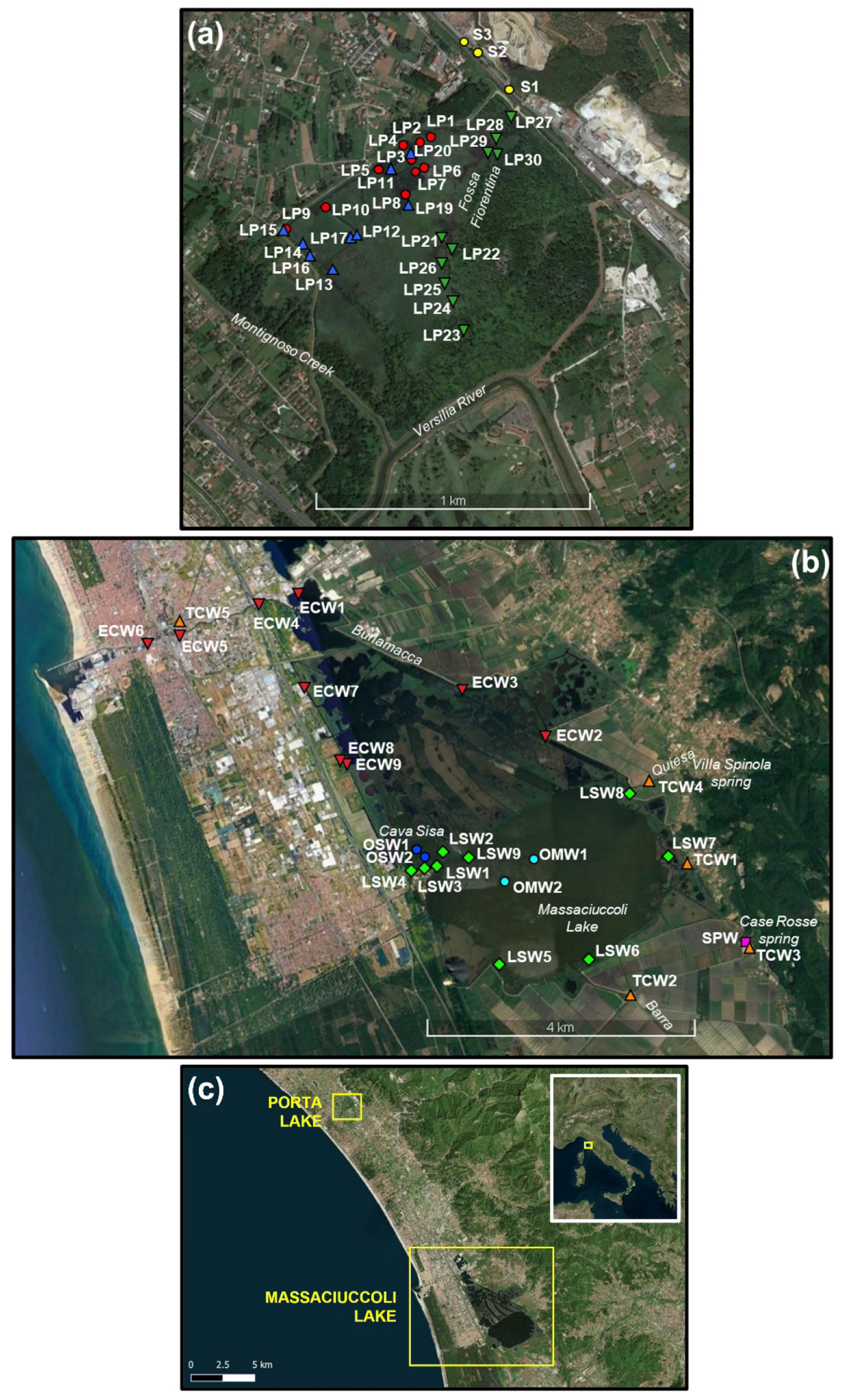
2.1. Study Areas

2.1.1. Porta Lake

Porta Lake (ca. 82 ha) is a wetland located between the coastline (ca. 2.5 km from the sea) and the Apuan Alps. The rocky substratum is made of Tuscan Units formations (Macigno sandstones) overlaid by marine to littoral alternations of clay and sand and alluvial deposits [39] and references therein, whereas the dominant soil class in the area is represented by histosols [40]. Lake waters are fed by three springs located at the base of the reliefs on the northeastern margin of the lake (Figure 1a) characterized by widely varying flow rates, ranging from 20.5 to 50 L/s [41]. The spring waters enter the lake through a channel, named Fossa Fiorentina, and slowly flow through excavated channels and ponds until they leave the lake on its southwestern margin, merging the Montignoso creek and, finally, the Versilia River (Figure 1a). A large portion of the wetland is characterized by the presence of wooded areas (dominated by Salix alba and Alnus glutinosa) and Phragmites australis reeds, the latter being affected by reed die-back syndrome (RDBS), e.g., [42,43,44,45], since 2016, determining a high accumulation of organic material at the lake bottom, oxygen depletion and emissions of H₂S-rich gases [37].

2.1.2. Massaciuccoli Lake

Massaciuccoli Lake is included in the Migliarino–San Rossore–Massaciuccoli Regional Park, representing an area of international importance under the Ramsar Convention, being recognized as a Site of Importance of the European Community [39], and thus it is regarded as one of the most important wetlands in Italy [46]. It includes (i) a main open-water basin with an average depth of 2 m [39], (ii) a secondary excavated basin (Cava Sisa) in correspondence of a former quarry, with a maximum depth of 24 m [46] and references therein, (iii) an extensive marsh area surrounding the lake northward and eastward and consisting of several pools of different sizes, artificial canals and basins (Figure 1b). The lake waters are fed by precipitation, groundwaters and a series of natural and artificial tributaries, flowing from the mountain belt or fed by water springs (e.g., Case Rosse, Villa Spinola). The surface water network drains agricultural, industrial and urban areas upstream of the lake basin and includes Barra, Fossa Nuova and Quiesa channels (Figure 1b) [47]. The lake has a main emissary, i.e., the Burlamacca canal, that, flowing through the city of Viareggio, directly connects Massaciuccoli Lake to the sea (Figure 1b). The lake waters are affected by severe eutrophication related to water inputs from the drainage of the farmlands and treatment plants of urban wastewater that produce a dramatic reduction of macroalgae and submerged macrophytes and an excessive growth of phytoplankton [46,48,49]. Reed beds are only discontinuously present along the lake and channel shores [50]. Such an environment is thus characterized by variable conditions of water depth, temperature, pH, salinity and redox state (dictated by the availability of free oxygen) along both vertical and lateral profiles, also depending on the contribution of brackish waters due to the marine ingression and fresh, meteoric and runoff waters from the hinterland.

2.2. Water and Dissolved Gas Sampling

Sampling campaigns were performed in August and December 2020 at Porta Lake and in November 2020 at Massaciuccoli Lake. Sampling activities were carried out between 10:00 and 16:00. Wind speed during sampling campaigns was, on average, around 2.5 m/s (Weather Underground company, San Francisco, CA, USA; https://www.wunderground.com). The coordinates of the sampling sites were recorded using a portable GPS (Garmin^® GPSMAP 62, Garmin^®, Olathe, KS, USA). Water temperature, pH and Eh values were measured directly in the field through a CRISON MM 40+ multiparameter probe. Sampling procedures within the lakes were performed from a small boat, with the exception of few sampling sites at Porta Lake (from LP21 to LP30), which were collected from the lake shores, mostly in areas of dense vegetation and stagnant water (Figure 1a). Water and dissolved gas sampling were carried out in lakes and canals within 5 cm of the water–air interface. Two aliquots were collected for the analysis of water chemical and isotopic composition as follows: (i) one aliquot of unfiltered water was collected in a 125 mL polyethylene bottle for the analysis of major anions, and (ii) one aliquot of filtered (0.45 µm) and acidified (with 0.5 mL of Suprapur^® HCl 30%) water was collected in a 50 mL polyethylene bottle for the analysis of major cations. At Massaciuccoli Lake, two further water aliquots were sampled as follows: (i) in 250 mL polyethylene bottles, containing SrCl₂ and NaOH to precipitate the dissolved carbonate species as SrCO₃, for isotope analysis of total dissolved inorganic carbon (δ¹³C-TDIC) [51] and (ii) in 15 mL plastic tubes, after filtration (0.45 µm), for the analysis of stable isotopes of water at selected sites (SPW, TCW2, TCW3, TCW4, TCW5, LSW4, LSW5, LSW7, LSW8, OMW1, OMW2, OSW1, ECW2, ECW3, ECW8 and ECW9). Dissolved gases were sampled by using pre-evacuated glass flasks with a PTFE stopcock. The flask was submerged down to the sampling depth and the stopcock was opened, allowing the water to enter the flask. The dissolved gases partially exsolved in the headspace due to the pressure drop. The flask was filled by 3/4 of its volume with water, before closing the stopcock [52,53]. Within Massaciuccoli Lake system, waters and dissolved gases were further collected along vertical profiles at three selected sites from surface to bottom using the single hose method described in Tassi et al. [54].

2.3. Chemical and Isotopic Analysis of Water and Dissolved Gases

The chemical composition of water was analyzed by (i) acidimetric titration (HCl 0.01 N) for the determination of HCO₃⁻ and (ii) ion chromatography, using Metrohm 761 and Metrohm 861 chromatographs for the determination of major anions (Cl⁻, SO₄²⁻, NO₃⁻, Br⁻ and F⁻) and cations (Na⁺, K⁺, Ca²⁺ and Mg²⁺), respectively. The analytical error was <5%. The ¹⁸O/¹⁶O and D/¹H isotopic ratios of water (expressed as δ¹⁸O-H₂O and δD-H₂O in‰ vs. V-SMOW) were determined using a Picarro L2130-i analyzer based on cavity ring-down spectroscopy (CRDS). The analysis of the δ¹³C-TDIC (expressed in‰ vs. V-PDB) was performed by mass spectrometry (MS) using a Finnigan MAT252 instrument on CO₂ recovered after the reaction of SrCO₃ with anhydrous phosphoric acid following the procedure described by Salata et al. [55] and a two-step extraction and purification procedure as described in Venturi et al. [56]. The analytical error and the reproducibility for δ¹³C-TDIC analysis were ±0.05‰ and ±0.1‰, respectively.

The chemical compositions of dissolved gases in the headspace of the sampling flask (CO₂, N₂, Ar + O₂, H₂ and He) were determined using a Shimadzu 15A gas chromatograph equipped with a 5 m long stainless steel column packed with Chromosorb PAW 80/100 mesh and a thermal conductivity detector (TCD), whereas CH₄ was analyzed using a Shimadzu 14A gas chromatograph equipped with a 10 m long stainless steel column packed with Chromosorb PAW 80/100 mesh coated with 23% SP 1700 and a flame ionization detector (FID). Argon and O₂ were analyzed using a Thermo Focus gas chromatograph equipped with a 30 m long capillary molecular sieve column and a TCD. The analytical error for GC analysis was <5% [54] and references therein. The concentrations of dissolved gas species were determined as the sum of the (i) number of moles of each gas in the headspace (n_i,g), calculated according to the ideal gas law at 20 °C (i.e., laboratory temperature) considering the partial pressures determined by gas chromatography (P_i), and the volume of the flask headspace (V_gas) and (ii) the number of moles of each gas remaining in the liquid (n_i,l), calculated according to Henry’s law, assuming that equilibrium was attained within the flask between the separated gas phase and the liquid, e.g., [54,57,58,59]. The ¹³C/¹²C isotopic ratios of CO₂ and CH₄ (expressed as δ¹³C-CO₂ and δ¹³C-CH₄, respectively, in‰ vs. V-PDB) in the headspace of the sampling flask were analyzed by CRDS using a Picarro G2201-i analyzer. The δ¹³C-CO₂ values were corrected considering the enrichment factor for gas–water isotope equilibrium between gaseous and dissolved CO₂ [56,60].

The chemical and isotopic analyses were carried out respectively by the Laboratory of Fluid Geochemistry and Laboratory of Stable Isotopes (Department of Earth Science, University of Florence), respectively, with the sole exception of the determination of δ¹³C-TDIC, which was carried out at the Laboratory of Fluids Geochemistry of the INGV, Sezione di Napoli, Osservatorio Vesuviano.

2.4. Diffusive Flux Calculation

The CO₂ and CH₄ diffusive fluxes at the water–air interface (ΦCO₂ and ΦCH₄, respectively) were determined on the basis of the measured dissolved gas concentrations (C_i,w, in mol/L), according to the thin boundary layer (TBL) model [61] as follows:

$${\Phi }_i=\beta k_i\left(C_{i,w}-C_{i,eq}\right)$$

(1)

where C_i,eq is the dissolved gas concentration calculated assuming equilibrium with the atmosphere (based on gas solubilities as a function of temperature and salinity [62]), β is the chemical enhancement applicable for CO₂ only (see below) and k_i is the gas transfer velocity (in cm h⁻¹). The k_i values were estimated as follows:

$$k_i=k_{600,i}{\left(\frac{S{c}_i}{600}\right)}^x$$

(2)

where (i) k_600,i is the k_i value for each gas normalized to 600, (ii) x is dependent upon the roughness of the water surface (−0.67 or −0.5 for wind speed <3 m s⁻¹ or >3 m s⁻¹, respectively [63]) and (iii) Sc_i is the Schmidt number. The Sc_i values were calculated for each gas based on temperature, according to the fourth order polynomial fits proposed by Wanninkhof [62]. The k_600,i values were calculated from local wind speed using the following empirical relationships [63,64]:

$$k_{600,i}=0.23U_{10}{}^2+0.1U_{10}$$

(3)

$$k_{600,i}=0.72U_{10}$$

(4)

where U₁₀ is the wind speed at a height of 10 m. The latter was calculated from average wind speed recorded during the sampling campaigns (Weather Underground company, San Francisco, CA, USA; https://www.wunderground.com) as described in Crusius and Wanninkhof [63] and references therein.

The chemical enhancement factor β for the determination of ΦCO₂ values was computed according to Hoover and Berkshire [65] and Wanninkhof and Knox [66] as follows:

$$\beta =\frac{\tau }{\left(\tau -1\right)+\frac{tanh\left[{\left(r\tau D^{-1}\right)}^{0.5}D{k}_{C{O}_2}^{-1}\right]}{\left[{\left(r\tau D^{-1}\right)}^{0.5}D{k}_{C{O}_2}^{-1}\right]}}$$

(5)

where: (i) D is the molecular diffusivity (in cm²/s), calculated as $D=14.6836\times {10}^{-5}\times {\left[\frac{\left(273.15+t\left(°C\right)\right)}{217.2056}-1\right]}^{1.997}$ [67] ; (ii) r (in s⁻¹) is the combined rate constant for the hydration of CO₂, calculated as $r=r_1+r_2{K}_w^{*}{a}_H^{-1}$, where r₁ (in s⁻¹) and r₂ (in Lmol⁻¹s⁻¹) are the CO₂ hydration rate and the CO₂ hydroxylation rate constants, respectively [68], K_w* is the equilibrium constant for water and a_H is the activity coefficient for the hydrogen ion; (iii) $\tau =1+\frac{a_H^2}{\left(K{\text{'}}_{1}K{\text{'}}_2+K{\text{'}}_1{a}_H\right)}$, where K′₁ and K′₂ are the first and second equilibrium constants for carbonic acid, respectively [69].

The overall diffusive flux in terms of CO₂ equivalents (ΦCO_2eq) was calculated as:

$$\Phi C{O}_{2eq}=\Phi C{O}_{2eq}+GW{P}_{CH4}\times \Phi C{H}_4$$

(6)

where GWP_CH4 is the global warming potential value of CH₄ over a 100-year time horizon (i.e., 28 [10]).

3. Results

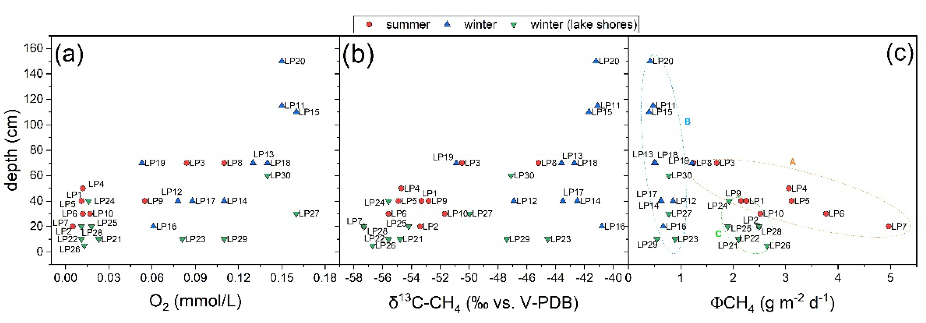
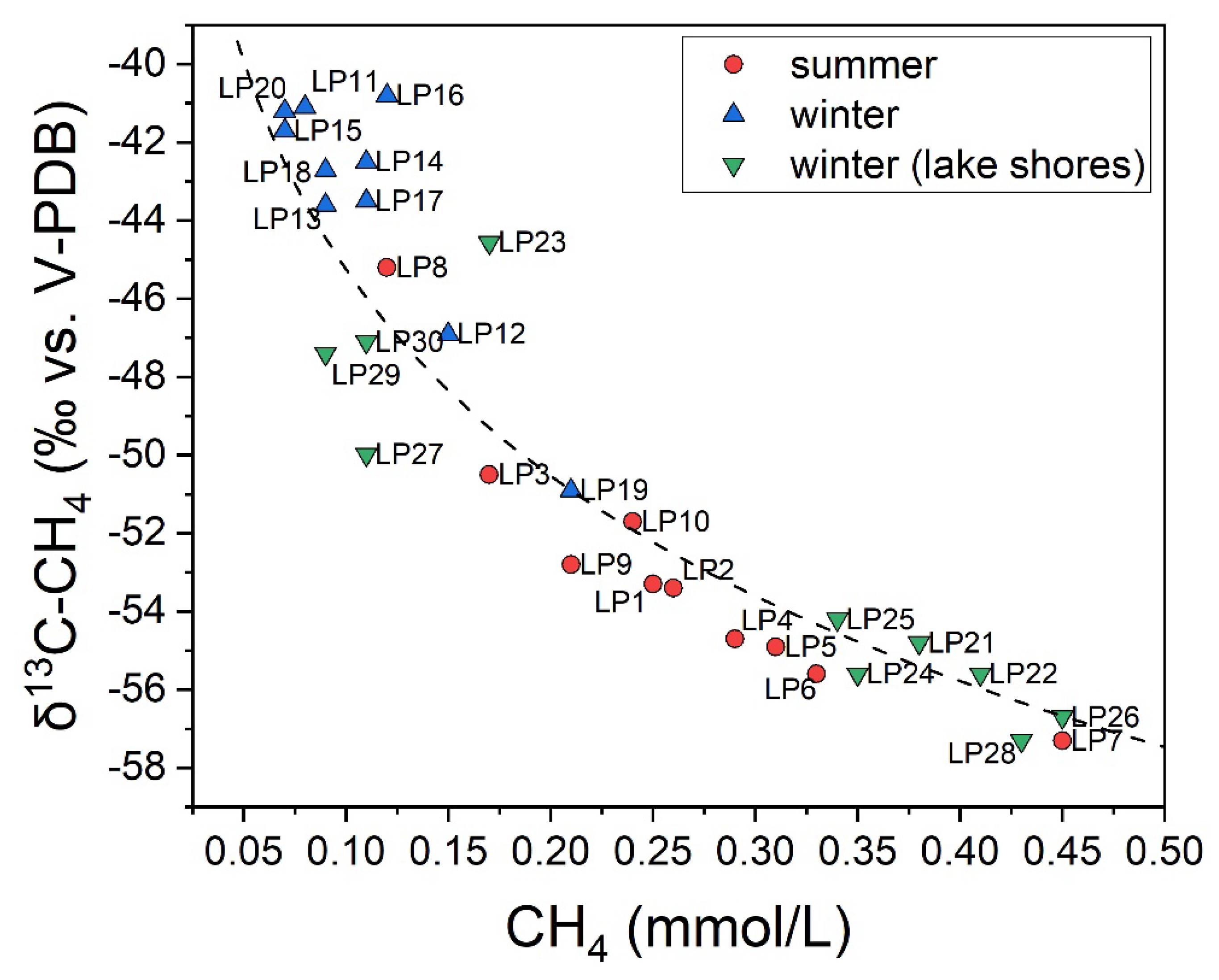
3.1. The Chemical Features of Porta Lake

Porta Lake waters were characterized by comparable pH values in summer and winter, i.e., ranging from 7.18 to 8.11 and from 7.17 to 7.78, respectively (

Table 1. Water column depth (w.c.d., in cm), temperature (in °C), pH, redox potential (Eh, in mV) and chemical composition of the main solutes in water samples (in mg/L) from Porta Lake. TDS (total dissolved solids, in mg/L) values are also reported.

	ID	E	N	w.c.d.	T	pH	Eh	HCO3	Cl	SO4	Na	K	Ca	Mg	NH4	NO3	F	Br	TDS
summertime	LP1	593756	4872054	40	23.7	7.41	−153	215	27	328	16	1.7	163	32	0.33	2.1	0.76	0.09	787
	LP2	593716	4872032	20	25.6	7.18	−295	204	24	301	16	2.0	153	32	0.23	0.11	0.33	0.08	733
	LP3	593687	4871974	70	26.7	7.4	89	201	26	328	16	1.7	161	32	0.08	0.61	0.44	0.09	768
	LP4	593661	4872021	50	28.7	7.47	−32	192	26	325	17	2.5	160	33	0.11	0.06	0.49	0.08	755
	LP5	593573	4871929	40	27.1	7.4	−66	205	26	323	17	2.2	162	32	0.16	0.40	0.33	0.09	768
	LP6	593732	4871939	30	31.2	8.11	−129	192	27	327	17	1.9	160	32	0.27	0.25	0.47	0.09	757
	LP7	593704	4871926	20	30.1	7.54	−192	205	26	320	17	1.4	161	32	0.38	0.04	0.32	0.08	763
	LP8	593666	4871844	70	28.1	7.64	20	199	27	328	17	2.2	163	33	0.09	0.45	0.36	0.09	769
	LP9	593226	4871708	40	27.7	7.3	−51	201	27	307	17	1.6	160	32	0.20	0.14	0.61	0.09	746
	LP10	593377	4871788	30	28.5	7.4	−120	201	27	334	16	2.1	160	32	0.21	0.13	0.38	0.09	773
wintertime	LP11	593613	4871927	115	11.3	7.4	96	217	20	281	19	1.3	150	30	0.09	1.97	0.24	0.06	722
	LP12	593493	4871693	40	10.3	7.5	35	216	20	272	19	2.3	147	30	0.08	1.46	0.23	0.15	708
	LP13	593402	4871555	70	9.4	7.4	87	204	18	273	18	2.1	130	27	0.08	0.37	0.18	0.09	672
	LP14	593298	4871649	40	10.0	7.55	24	220	19	245	17	2.4	138	26	0.11	1.47	0.22	0.08	670
	LP15	593219	4871708	110	10.2	7.48	95	221	22	285	20	3.6	151	30	0.11	1.86	0.36	0.09	735
	LP16	593325	4871615	20	9.6	7.49	12	219	19	215	18	2.7	118	24	0.37	0.82	0.80	0.09	618
	LP17	593473	4871679	40	10.5	7.45	19	220	19	258	19	1.2	137	30	0.28	1.42	0.24	0.06	686
	LP18	593376	4871786	70	10.6	7.54	52	218	19	274	21	4.3	143	31	0.13	1.60	0.21	0.08	713
	LP19	593680	4871797	70	10.8	7.53	4	215	21	261	20	2.6	136	30	0.53	1.93	0.20	0.08	688
	LP20	593684	4871988	150	11.6	7.5	81	215	19	257	19	1.6	135	30	0.19	2.68	0.28	0.08	680
	LP21	593805	4871686	10	9.5	7.2	−77	331	46	129	25	33	105	33	0.51	1.02	0.13	0.17	703
	LP22	593837	4871648	10	7.7	7.25	−80	386	36	39	22	7.9	95	31	0.79	0.48	0.18	0.12	618
	LP23	593885	4871350	10	8.2	7.52	12	398	70	30	44	7.1	95	34	0.27	0.04	0.08	0.22	678
	LP24	593841	4871464	40	9.4	7.5	−54	432	33	61	32	5.7	116	34	0.73	0.02	0.17	0.14	715
	LP25	593814	4871521	20	9.8	7.6	−31	322	26	145	25	4.4	122	31	0.54	0.02	0.19	0.12	676
	LP26	593800	4871601	5	11.2	7.6	−98	272	23	188	20	3.8	128	30	0.61	3.26	0.26	0.11	669
	LP27	594047	4872130	30	16.1	7.17	85	212	24	363	18	2.7	177	34	0.05	7.68	0.43	0.09	839
	LP28	593996	4872049	20	10.8	7.71	−140	262	25	217	22	4.9	124	29	0.43	0.70	0.45	0.04	686
	LP29	593972	4872003	10	12.0	7.78	27	221	19	323	21	3.0	157	34	0.04	5.08	0.21	0.08	784
	LP30	593997	4871997	60	16.1	7.69	53	217	26	337	24	3.0	169	33	0.04	7.20	0.32	0.05	816
spring waters	S1	594043	4872228		17.0	7.8	155	212	32	286	23	2.3	156	29	0.02	7.2	0.45	0.09	748
	S2	593923	4872362		17.5	7.92	141	195	20	375	12	2.2	171	33	0.02	7.0	0.39	0.05	814
	S3	593876	4872404		18.0	7.76	160	195	19	356	12	2.5	171	33	0.02	6.7	0.42	0.04	795

), whereas TDS (total dissolved solids) values were from 733 to 787 mg/L in summer and from 618 to 839 mg/L in winter (Table 1). The Eh values ranged from −295 to 96 mV, with the lowest values recorded in August (Table 1). Water temperatures were from 23.7 to 31.2 °C in summer and from 7.7 to 16.1 °C in winter. In the sampling sites, the lake depth varied from 20 to 70 cm in summer and from 5 to 150 cm in winter, with an increase in the water column depth of more than 40 cm in December with respect to that of August (LP10, LP18; Table 1). The chemical composition of Porta Lake waters was dominated by the Ca²⁺-SO₄²⁻ facies, in agreement with the composition of spring waters feeding the lake (S1, S2 and S3), with the sole exception of few samples collected in winter (i.e., LP21, LP22, LP23, LP24, LP25 and LP26) and located in the easternmost margin of the lake (Figure 1a) which displayed a Ca²⁺-HCO₃⁻ geochemical facies. The lake waters were enriched in NH₄⁺ and generally depleted in NO₃ with respect to the spring waters (Table 1). Fluoride and Br⁻ concentrations were relatively low (≤0.76 and ≤0.2 mg/L, respectively).

Dissolved gases were dominated by N₂, generally followed by either CH₄ or O₂, whereas CO₂ was, in most samples, the third most abundant compound (

Table 2. Chemical composition (in mmol/L) of the main dissolved gases from Porta Lake. The isotopic composition of carbon in CO₂ and CH₄ (δ¹³C-CO₂ and δ¹³C-CH₄, respectively, in ‰ vs. V-PDB) is also reported, as well as the CO₂, CH₄ and CO_2eq diffusive fluxes (ΦCO₂, ΦCH₄ and ΦCO_2eq, respectively, in g m⁻² d⁻¹).

ID	CO2	N2	Ar	CH4	O2	δ13C-CO2	δ13C-CH4	ΦCH4	ΦCO2	ΦCO2eq
LP1	0.09	0.53	0.013	0.25	0.011	−21.5	−53.3	2.25	16.6	79.6
LP2	0.14	0.51	0.013	0.26	0.005	−20.9	−53.4	2.49	20.6	90.4
LP3	0.11	0.52	0.013	0.17	0.084	−18.7	−50.5	1.69	24.1	71.3
LP4	0.09	0.53	0.014	0.29	0.012	−20.8	−54.7	3.06	23.8	110
LP5	0.08	0.49	0.012	0.31	0.011	−21.3	−54.9	3.11	17.0	104
LP6	0.07	0.51	0.013	0.33	0.012	−21.8	−55.6	3.77	52.8	158
LP7	0.13	0.49	0.013	0.45	0.005	−22.1	−57.3	4.97	43.5	183
LP8	0.13	0.52	0.013	0.12	0.11	−17.6	−45.2	1.24	46.4	81.2
LP9	0.09	0.55	0.014	0.21	0.055	−21.3	−52.8	2.15	17.0	77.2
LP10	0.09	0.52	0.013	0.24	0.017	−21.4	−51.7	2.52	20.9	91.5
LP11	0.11	0.68	0.017	0.08	0.15	−18.4	−41.1	0.472	9.73	23.0
LP12	0.08	0.71	0.018	0.15	0.078	−18.5	−46.9	0.853	6.94	30.8
LP13	0.12	0.69	0.018	0.09	0.13	−18.7	−43.6	0.495	9.50	23.3
LP14	0.09	0.67	0.017	0.11	0.11	−18.7	−42.5	0.619	8.57	25.9
LP15	0.08	0.69	0.017	0.07	0.16	−18.2	−41.7	0.397	6.68	17.8
LP16	0.05	0.72	0.018	0.12	0.061	−18.6	−40.8	0.665	3.13	21.7
LP17	0.07	0.69	0.017	0.11	0.088	−18.4	−43.5	0.630	5.44	23.1
LP18	0.09	0.68	0.017	0.09	0.14	−18.4	−42.7	0.518	8.82	23.3
LP19	0.11	0.67	0.017	0.21	0.053	−19.7	−50.9	1.22	11.4	45.5
LP20	0.08	0.69	0.018	0.07	0.15	−19.8	−41.2	0.418	7.69	19.4
LP21	0.13	0.65	0.016	0.38	0.023	−23.3	−54.8	2.10	7.83	66.5
LP22	0.14	0.66	0.016	0.41	0.011	−24.2	−55.6	2.11	8.20	67.3
LP23	0.15	0.65	0.017	0.17	0.081	−26.7	−44.6	0.892	13.7	38.7
LP24	0.14	0.65	0.016	0.35	0.016	−23.9	−55.6	1.92	13.3	67.2
LP25	0.12	0.66	0.017	0.34	0.018	−21.9	−54.2	1.90	13.1	66.3
LP26	0.16	0.66	0.017	0.45	0.013	−21.1	−56.7	2.65	20.4	94.6
LP27	0.09	0.65	0.016	0.11	0.16	−18.0	−50.0	0.772	7.18	28.8
LP28	0.11	0.66	0.016	0.43	0.011	−21.9	−57.3	2.49	14.7	84.5
LP29	0.08	0.65	0.016	0.09	0.11	−18.3	−47.4	0.545	11.6	26.9
LP30	0.07	0.65	0.016	0.11	0.14	−18.9	−47.1	0.772	11.7	33.3

). Dissolved oxygen concentrations were higher in winter (from 0.011 to 0.16 mmol/L) than in summer (from 0.005 to 0.11 mmol/L). On the contrary, CH₄ showed, on average, higher concentrations in summer (mean: 0.26 mmol/L) than in winter (mean: 0.20 mmol/L). The measured N₂/Ar ratios were consistent with those of air-saturated water (ASW), i.e., around 40. The δ¹³C-CH₄ values ranged from −57.3 to −40.8‰ vs. V-PDB, whereas those of CO₂ values varied from −26.7 to −17.6‰ vs. V-PDB (Table 2).

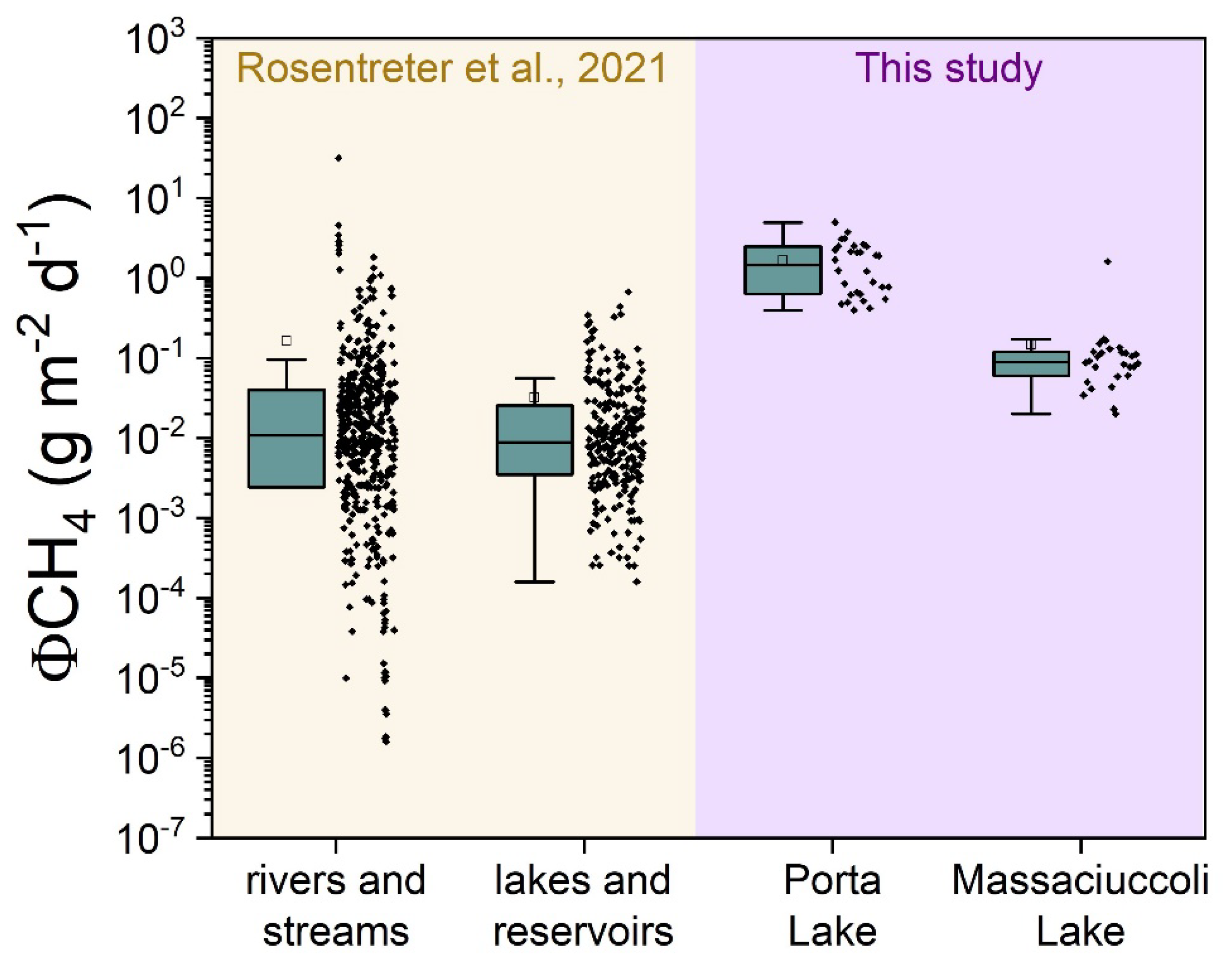
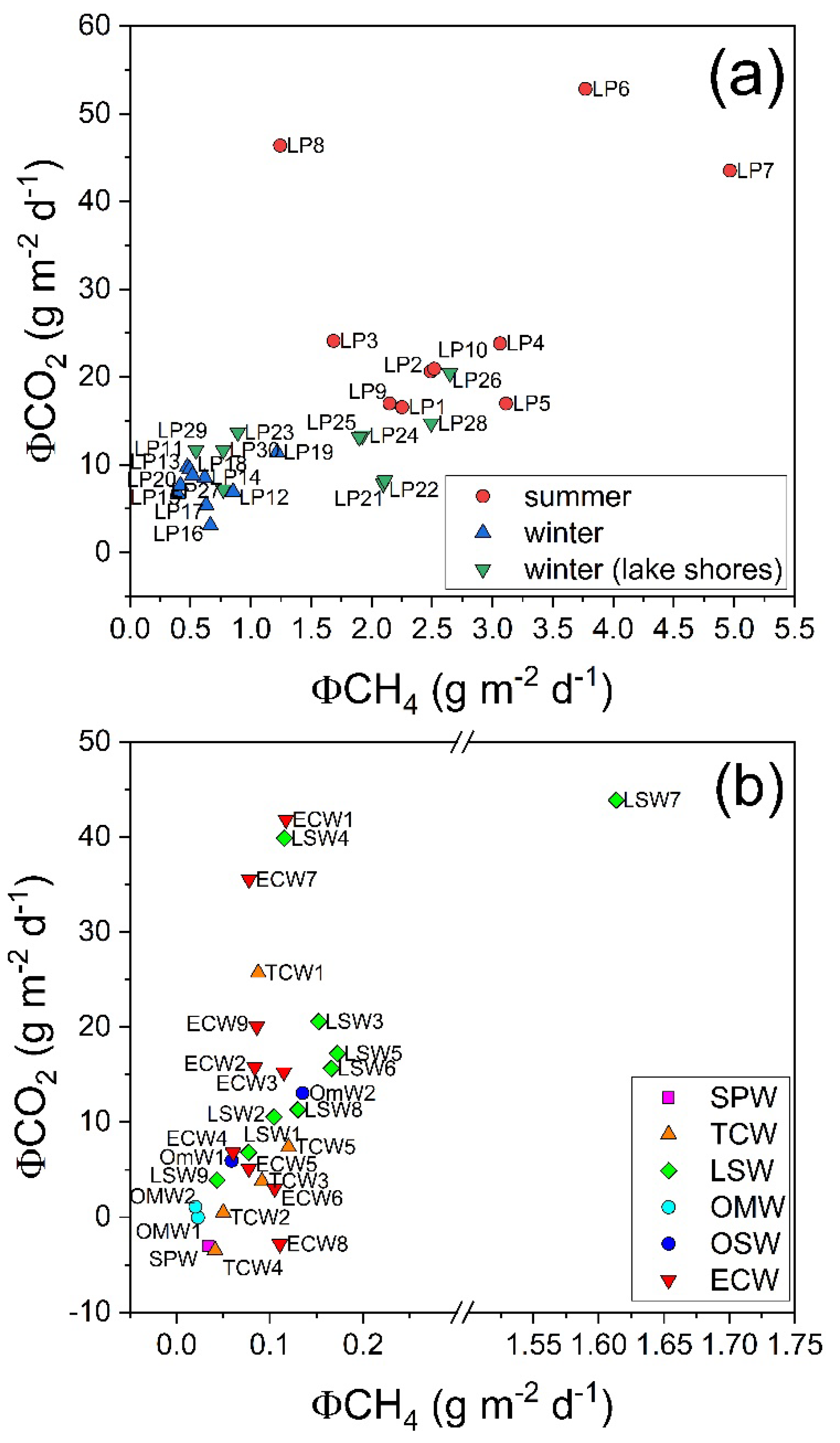
3.2. CH₄ and CO₂ Diffusive Fluxes at Porta Lake

The CH₄ and CO₂ diffusive fluxes at the water–air interface calculated according to the TBL model are reported in Table 2. The ΦCH₄ values varied from 1.24 (LP8) to 4.97 (LP7) g CH₄ m⁻² day⁻¹ in summer, whereas lower values were measured in winter, ranging from 0.397 (LP15) to 2.65 (LP26) g CH₄ m⁻² day⁻¹. Similarly, the calculated ΦCO₂ values were positive, with higher values in summer (from 16.6 to 52.8 g CO₂ m⁻² day⁻¹) with respect to winter (from 3.13 to 20.4 g CO₂ m⁻² day⁻¹). In terms of CO₂ equivalents, diffusive fluxes from Porta Lake varied from 71 (LP3) to 183 (LP7) g CO_2eq m⁻² in summer and from 18 (LP15) to 95 (LP26) g CO_2eq m⁻² in winter.

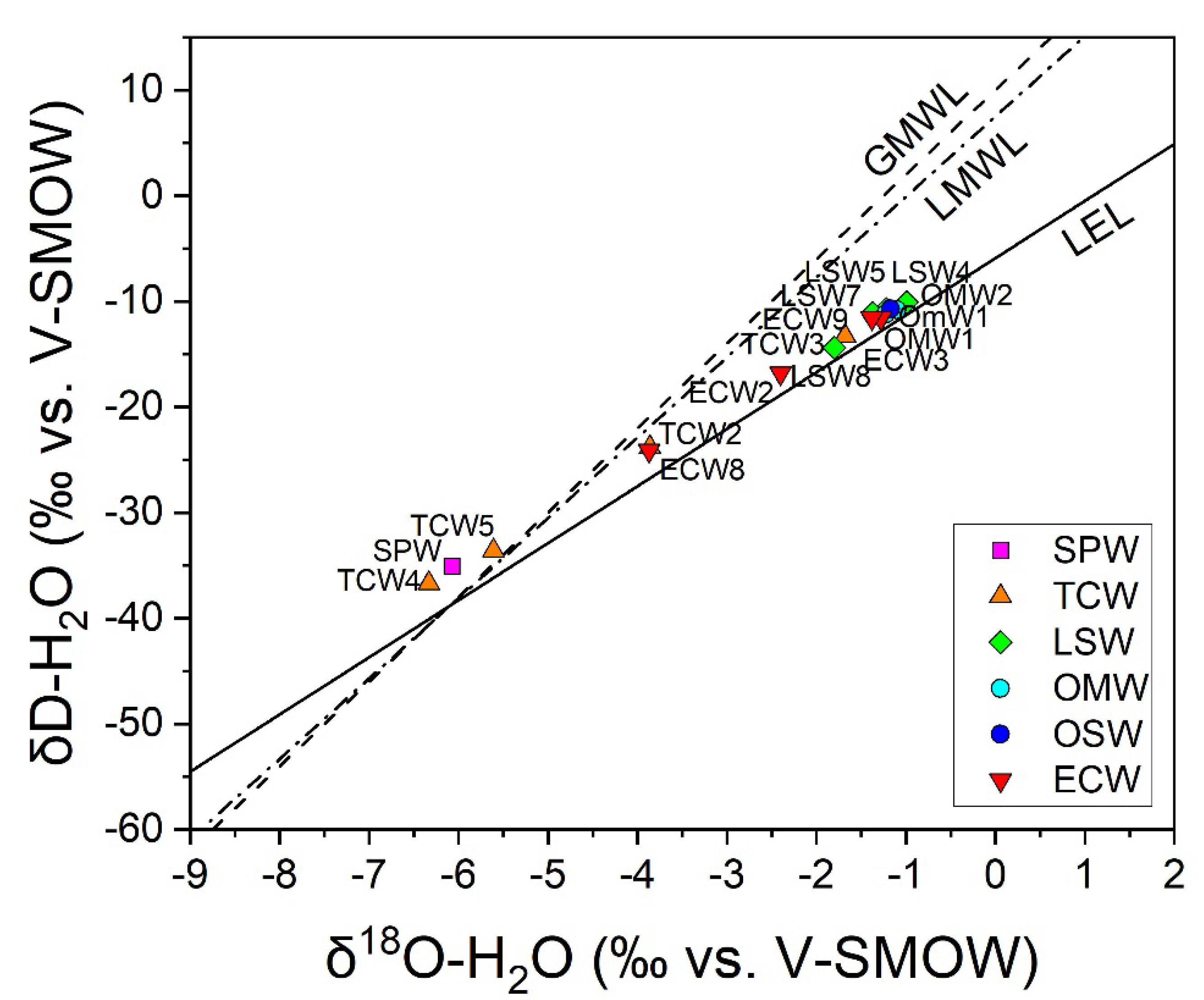
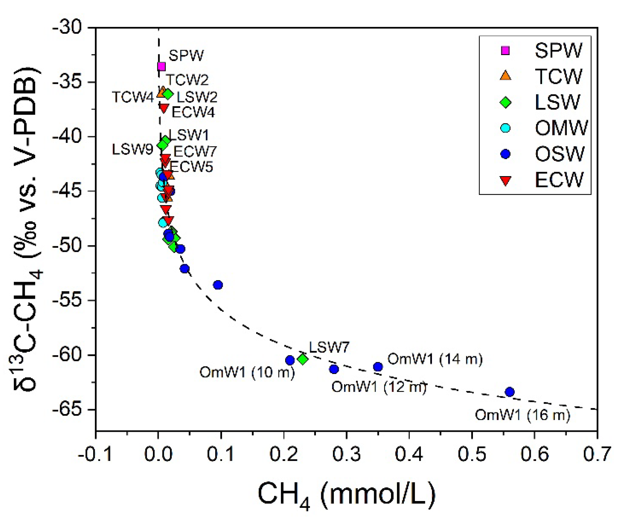
3.3. The Chemical Features of Massaciuccoli Lake System

The waters collected from Massaciuccoli Lake system referred to a wide variety of environments, i.e., open waters from both (i) the main Massaciuccoli Lake basin (OMW) and (ii) the excavated Cava Sisa basin (OSW), (iii) waters collected close to the lake shores (LSW), (iv) Case Rosse spring water (SPW), which is one of the springs feeding the lake [47], (v) several tributary channels discharging waters in Massaciuccoli Lake or in the Burlamacca canal (TCW) and (vi) emissary channels (ECW), including the Burlamacca canal (Figure 1b).

The collected surface waters were characterized by pH values ranging from 7.8 to 8.5 and T from 13.7 to 17.4 °C (

Table 3. Water column depth (w.c.d., in m), temperature (in °C), pH, redox potential (Eh, in mV) and chemical composition of the main solutes in water samples (in mg/L) from Massaciuccoli Lake. TDS (total dissolved solids, in mg/L) values are also reported, along with the isotopic composition of carbon in total dissolved inorganic carbon (δ¹³C-TDIC, in ‰ vs. V-PDB) and of oxygen and hydrogen in water (δ¹⁸O-H₂O and δD-H₂O, in ‰ vs. V-SMOW).

	ID	E	N	w.c.d.	T	pH	Eh	HCO3	Cl	SO4	Na	K	Ca	Mg	NH4	NO3	F	Br	TDS	δ18O−H2O	δD−H2O	δ13C−TDIC
spring water	SPW	609910	4853354	0	15.4	7.77	645	263	40	13	24	1.7	85	6.2	0.04	6.1	0.26	0.11	439	−6.07	−35.1	−14.75
tributary channels	TCW1	609028	4854555	2	17.21	8.41	117	206	525	395	361	15	141	61	0.13	0.39	0.52	1.7	1707			−13.6
	TCW2	608185	4852544	1	14.3	7.85	223	451	726	450	396	8.5	222	91	0.81	11	0.45	3.3	2360	−3.86	−23.8	−13.03
	TCW3	609931	4853285	1	14.1	7.93	221	222	811	222	423	20	110	68	0.16	0.2	0.39	3	1880	−1.68	−13.3	−12.9
	TCW4	608460	4855717	0.5	16.5	8.11	209	166	20	281	10	0	141	11	0.05	6.3	0.39	0.06	636	−6.33	−36.7	−13.79
	TCW5	601245	4858083	1.5	16.3	8.16	201	274	246	178	141	11	115	26	1.72	31	0.5	0.73	1025	−5.61	−33.6	−13.75
lake shores	LSW1	605253	4854472	3	16.1	8.1	209	212	981	449	622	26	132	99	0.32	0.21	0.33	2.5	2524			−11.7
	LSW2	605329	4854662	3	15.9	8.18	179	185	998	433	611	26	128	97	0.25	0.26	0.61	2.6	2482			−12.6
	LSW3	605053	4854417	3	17.1	8.25	127	209	1040	431	627	26	140	100	0.2	0.21	0.42	2.4	2576			−12.9
	LSW4	604864	4854403	1.8	17	8.45	135	198	984	452	614	25	131	98	0.23	0.23	0.45	2.4	2505	−0.99	−10.1	−13.5
	LSW5	606212	4852985	0.8	14.5	7.86	164	224	993	366	610	31	138	95	0.24	1.3	0.61	2.9	2462	−1.22	−10.7	−12.4
	LSW6	607547	4853088	0.8	14.5	7.87	223	240	989	399	591	27	136	94	0.23	0.13	0.37	4.1	2481			−12.84
	LSW7	608772	4854627	1	16.1	7.98	−179	231	1078	297	618	32	138	98	0.3	0	0.45	4.3	2497	−1.37	−11.1	−13.06
	LSW8	608132	4855571	1	15.4	7.82	184	281	1125	267	593	27	152	96	0.48	0.24	0.71	3.9	2546	−1.8	−14.4	−13.82
	LSW9	605717	4854577	2.5	14.8	8.22	195	209	1039	246	612	26	130	96	0.14	0.15	0.42	3.8	2363			−14.23
emissary channels	ECW1	603052	4858611	1	17.4	8.36	133	211	1730	495	1020	42	172	147	0.13	0.28	0.44	3.6	3822			−14.1
	ECW2	606877	4856416	0.7	16	7.89	210	219	1166	302	611	28	135	92	0.11	0.38	0.66	4	2558	−2.4	−16.8	−13.13
	ECW3	605588	4857131	0.7	16.8	8.12	211	219	1515	304	763	47	150	118	0.18	0.36	0.54	5	3122	−1.28	−11.6	−12.55
	ECW4	602446	4858415	1	16.5	8.29	202	219	1672	306	829	34	151	120	0.11	0.22	0.56	6.4	3338			−12.7
	ECW5	601273	4857944	1	16.2	8.37	208	227	1555	350	810	29	152	122	0.14	0.39	0.41	6.5	3252			−13.18
	ECW6	600820	4857784	1	16.1	8.2	196	231	1490	297	753	32	146	113	0.13	0.75	0.69	5.2	3069			−12.25
	ECW7	603180	4857119	0.7	16.3	8.38	193	241	1368	273	735	33	139	111	0.18	0.01	0.63	5.2	2906			−12.17
	ECW8	603748	4856001	0.7	15.7	8.15	201	323	727	121	389	22	116	64	0.38	17	0.51	2.6	1782	−3.87	−24.1	−14.51
	ECW9	603842	4855965	0.7	16.7	8.1	219	244	1274	263	664	29	138	103	0.15	0.42	0.46	5.5	2722	−1.38	−11.6	−12.98
main basin (Massaciuccoli lake)	OMW1 (0 m)	606696	4854546	3	14.1	7.77	214	220	996	320	590	28	129	90	0.22	0.02	0.39	4.1	2378	−1.22	−11.2	−13.78
	OMW1 (1 m)	606696	4854546		13.9	7.69	214	212	1245	331	634	23	143	99	0.23	0.04	0.32	4.2	2692			−16.79
	OMW1 (2 m)	606696	4854546		13.5	7.57	236	208	1196	255	639	22	138	101	0.23	0.01	0.39	5.1	2565			−16.68
	OMW1 (3 m)	606696	4854546		13.5	7.39	230	213	1312	307	639	27	140	100	0.25	0.13	0.44	5.4	2744			−16.71
	OMW2 (0 m)	606275	4854208	2.5	13.7	8.34	193	214	1261	296	629	28	138	99	0.2	0.01	0.48	4.8	2670	−1.1	−10.8	−13.91
	OMW2 (1 m)	606275	4854208		13.7	8.26	183	213	1225	285	632	25	143	99	0.2	0.04	0.56	4.3	2627			−13.34
	OMW2 (2 m)	606275	4854208		13.9	7.94	180	214	1213	289	638	24	139	100	0.23	0.12	0.51	4.1	2622			−13.51
	OMW2 (2.5 m)	606275	4854208		13.9	7.88	190	212	1209	284	626	23	138	98	0.13	0.22	0.47	3.9	2595			−13.55
Cava Sisa	OSW1 (0 m)	604945	4854675	16	15.1	8.2	188	213	1042	313	616	27	128	96	0.15	0.24	0.45	4.4	2440	−1.17	−10.7	−13.49
	OSW1 (1 m)	604945	4854675		14.8	8.14	164	212	1206	275	608	19	129	95	0.11	0.07	0.39	4.3	2549			−13.25
	OSW1 (2 m)	604945	4854675		14.8	8.08	149	212	1171	267	611	24	130	95	0.16	0.2	0.33	4.2	2515			−13.86
	OSW1 (4 m)	604945	4854675		14.7	8.12	138	211	1176	268	614	25	130	96	0.11	0.2	0.39	3.8	2525			−14.87
	OSW1 (6 m)	604945	4854675		14.7	8.14	137	217	1247	318	624	30	133	96	0.11	0.35	0.45	4.1	2670			−14.59
	OSW1 (8 m)	604945	4854675		14.7	8.14	146	207	1169	266	622	21	131	97	0.14	0.15	0.46	3.8	2518			−14.30
	OSW1 (10 m)	604945	4854675		14.5	8.16	−11	212	1252	288	601	24	128	95	0.14	0.2	0.49	3.9	2605			−16.33
	OSW1 (12 m)	604945	4854675		10.9	7.47	−202	272	1160	268	621	91	138	94	1.5	0.1	0.54	3.6	2650			−16.68
	OSW1 (14 m)	604945	4854675		10	7.35	−212	297	1170	267	577	29	143	92	2.03	0.08	0.57	3.7	2581			−16.70
	OSW1 (16 m)	604945	4854675		9.9	7.17	−215	314	1101	268	574	22	138	92	2.7	0.36	0.66	3.4	2516			−17.01
	OSW2	605069	4854569	15	16.5	8.2	163	209	1050	444	640	29	135	100	0.18	0.18	0.42	2.6	2610			−13.1

). The SPW sample was characterized by a Ca²⁺-HCO₃⁻ composition and TDS and Eh values of 439 mg/L and 645 mV, respectively. Nitrate was present at a relatively high concentration, i.e., 6.1 mg/L (Table 3). The isotopic composition of this spring was characterized by δ¹⁸O-H₂O and δD-H₂O values of −6.07 and −35.1 in‰ vs. V-SMOW, respectively, whereas the δ¹³C-TDIC value was −14.8‰ vs. V-PDB (Table 3). Conversely, the TCW samples showed TDS values ranging from 636 (TCW4) to 2360 (TCW2) mg/L and Eh values varying from 117 (TCW1) to 223 (TCW2) mV. They were characterized by a Na⁺-Cl⁻ composition, with the sole exception of TCW4 that showed Ca²⁺ and SO₄²⁻ as dominant cationic and anionic species (Table 3). The water column depth varied from 0.5 to 2 m. On average, the TCW samples were characterized by the highest NH₄⁺ and NO₃⁻ concentrations, up to 1.7 and 31 mg/L, respectively, in TCW5 (Table 3). The δ¹⁸O-H₂O and δD-H₂O values were ranging from −6.33 (TCW4) to −1.68 (TCW3)‰ vs. V-SMOW and from −36.7 (TCW4) to −13.3 (TCW3)‰ vs. V-SMOW, respectively (Table 3). The δ¹³C-TDIC values ranged from −13.8 (TCW4 and TCW5) to −12.9 (TCW3)‰ vs. V-PDB (Table 3).

On average, the ECW samples displayed higher TDS values, which ranged from 1782 (ECW8) to 3821 (ECW1) mg/L, and comparable Eh, varying from 133 (ECW1) to 219 (ECW9) mV, whilst the water column depth ranged from 0.7 to 1 m. The chemical composition of the ECW samples was Na⁺-Cl⁻, with significantly higher concentrations of Na⁺, Cl⁻, K⁺ and Br⁻ with respect to the TCW samples (Table 3). The NH₄⁺ and NO₃⁻ concentrations were up to 0.38 and 17 mg/L, respectively (ECW8). The isotopic composition of water in the ECW samples showed a relative enrichment in the heavier isotopes with respect to those of TCW, with δ¹⁸O-H₂O and δD-H₂O values varying from −3.87 (ECW8) to −1.28 (ECW3)‰ vs. V-SMOW and from −24.1 (ECW8) to −11.6 (ECW3 and ECW9)‰ vs. V-SMOW, respectively (Table 3). The δ¹³C-TDIC values ranged from −14.5 (ECW8) to −12.2 (ECW7)‰ vs. V-PDB (Table 3).

The surface waters from Massaciuccoli Lake (OMW) and Cava Sisa (OSW) were characterized by comparable TDS and Eh values, ranging from 2378 (OMW1) to 2670 (OMW2) mg/L and from 163 (OSW2) to 214 (OMW1) mV, respectively, and displayed a Na⁺-Cl⁻ geochemical facies (Table 3). The δ¹⁸O-H₂O and δD-H₂O values of surface waters were comparable between the two basins, ranging from −1.22 (OMW1) to −1.10 (OMW2)‰ vs. V-SMOW and from −11.2 (OMW1) to −10.7 (OSW1)‰ vs. V-SMOW, respectively (Table 3). Similarly, the carbon isotopic composition of TDIC was around −13.8‰ vs. V-PDB in OMW samples and −13.3‰ vs. V-PDB in the OSW samples (Table 3).

The water column depth significantly differed, varying from 2.5 to 3 m (OMW) and from 15 to 16 m (OSW). Different from the OMW sampling sites, a clear stratification was observed at OSW, with a sharp decrease in Eh, pH and T values between 8 and 12 m depth (Table 3). The bottom waters along the OSW profile were characterized by reduced conditions and higher NH₄⁺ concentrations (up to 2.7 mg/L) with respect to those measured in the shallower waters (≤0.14 mg/L). These concentrations were two orders of magnitude higher than those determined at the bottom of Massaciuccoli Lake main basin, i.e., 0.25 and 0.13 mg/L at OMW1 and OMW2, respectively (Table 3). The carbon isotopic composition of TDIC showed different trends along the vertical profile in the sampled sites. In Massaciuccoli Lake, OMW1 and OMW2 showed rather constant δ¹³C-TDIC values with depth, i.e., around −16.7 and −13.6‰ vs. V-PDB, respectively, with the sole exception of the OMW1 surface water that was enriched in the heavier isotope with respect to deeper waters (Table 3). At Cava Sisa, the δ¹³C-TDIC values showed a clear shift between 8 and 10 m depth, ranging from −14.9 to −13.3‰ vs. V-PDB in shallow waters and from −17.0 to −16.3‰ vs. V-PDB in deep waters (Table 3).

The LSW samples were characterized by TDS values ranging from 2363 (LSW9) to 2576 (LSW3) mg/L. Overall, the Eh values ranged from 127 (LSW3) to 223 (LSW6) mV, with the sole exception of the LSW7 sample, which displayed an Eh value of −179 mV; the water column depth varied from 0.8 to 3 m (Table 3). The chemical composition was dominated by Na⁺ and Cl⁻, with higher concentrations of NH₄⁺ and NO₃⁻ with respect to those recorded in the OMW and OSW surface water samples, i.e., up to 0.48 (LSW8) and 1.3 (LSW5) mg/L, respectively (Table 3). The isotopic composition of water was comparable with that of samples from open waters, the δ¹⁸O-H₂O and δD-H₂O values being from −1.80 (LSW8) to −0.99 (LSW4)‰ vs. V-SMOW and from −14.4 (LSW8) to −10.1 (LSW4)‰ vs. V-SMOW, respectively (Table 3). The δ¹³C-TDIC values ranged from −14.2 (LSW9) to −11.7 (LSW1)‰ vs. V-PDB (Table 3).

The chemical composition of dissolved gases was dominated by N₂ in all of the collected surface waters, with concentrations ranging from 0.54 (LSW4 and TCW3) to 0.66 (LSW8) mmol/L (

Table 4. Chemical composition (in mmol/L) of the main dissolved gases from Massaciuccoli Lake. The isotopic composition of carbon in CO₂ and CH₄ (δ¹³C-CO₂ and δ¹³C-CH₄, respectively, in ‰ vs. V-PDB) is also reported, as well as the CO₂, CH₄ and CO_2eq diffusive fluxes (ΦCO₂, ΦCH₄ and ΦCO_2eq, respectively, in g m^-2 d^-1).

ID	CO2	N2	Ar	CH4	O2	δ13C-CO2	δ13C-CH4	ΦCH4	ΦCO2	ΦCO2eq
SPW	0.01	0.59	0.014	0.005	0.25	−13.0	−33.6	0.034	−3.03	−2.07
TCW1	0.06	0.62	0.015	0.012	0.16	−15.6	−44.5	0.087	25.7	28.2
TCW2	0.02	0.55	0.013	0.0076	0.19	−17.1	−35.9	0.050	0.500	1.90
TCW3	0.03	0.54	0.013	0.014	0.18	−18.5	−45.6	0.092	3.78	6.35
TCW4	0.01	0.65	0.016	0.0058	0.31	−13.5	−36.1	0.041	−3.49	−2.33
TCW5	0.04	0.65	0.016	0.017	0.18	−15.4	−43.6	0.120	7.39	10.7
LSW1	0.04	0.58	0.014	0.011	0.19	−13.4	−40.4	0.077	6.82	8.98
LSW2	0.04	0.55	0.014	0.015	0.16	−15.9	−36.1	0.104	10.5	13.5
LSW3	0.06	0.63	0.015	0.021	0.15	−9.2	−48.7	0.152	20.6	24.8
LSW4	0.09	0.54	0.014	0.016	0.12	−22.0	−49.4	0.116	39.9	43.1
LSW5	0.09	0.63	0.016	0.026	0.15	−16.0	−49.3	0.172	17.2	22.1
LSW6	0.08	0.57	0.015	0.025	0.17	−17.5	−50.1	0.166	15.7	20.3
LSW7	0.15	0.63	0.016	0.23	0.056	−18.9	−60.4	1.61	43.9	89.0
LSW8	0.06	0.66	0.016	0.019	0.12	−15.4	−48.8	0.130	11.3	15.0
LSW9	0.05	0.63	0.016	0.0065	0.15	−15.3	−40.8	0.044	3.89	5.11
ECW1	0.10	0.56	0.013	0.016	0.13	−18.8	−47.6	0.117	41.8	45.1
ECW2	0.07	0.64	0.015	0.012	0.15	−17.4	−45.5	0.084	15.8	18.1
ECW3	0.06	0.61	0.015	0.016	0.17	−16.5	−45.1	0.115	15.3	18.5
ECW4	0.03	0.56	0.014	0.0085	0.16	−13.4	−37.3	0.060	6.79	8.48
ECW5	0.03	0.57	0.015	0.011	0.19	−14.8	−42.3	0.077	5.09	7.26
ECW6	0.03	0.63	0.015	0.015	0.15	−16.6	−43.4	0.105	3.01	5.96
ECW7	0.09	0.64	0.016	0.011	0.15	−14.7	−41.9	0.078	35.5	37.7
ECW8	0.01	0.61	0.015	0.016	0.18	−13.2	−44.8	0.111	−2.84	0.261
ECW9	0.07	0.61	0.016	0.012	0.19	−17.0	−46.6	0.086	20.0	22.4
OMW1 (0 m)	0.02	0.55	0.014	0.0035	0.19	−13.4	−44.5	0.023	−0.03	0.613
OMW1 (1 m)	0.04	0.58	0.014	0.0056	0.18	−12.7	−44.6
OMW1 (2 m)	0.05	0.64	0.016	0.0071	0.15	−13.0	−44.2
OMW1 (3 m)	0.08	0.63	0.016	0.0088	0.13	−13.6	−47.8
OMW2 (0 m)	0.02	0.57	0.014	0.0031	0.18	−12.7	−43.3	0.020	1.09	1.65
OMW2 (1 m)	0.04	0.59	0.015	0.0049	0.18	−13.7	−43.5
OMW2 (2 m)	0.06	0.54	0.014	0.0063	0.15	−13.9	−45.6
OMW2 (2.5 m)	0.10	0.56	0.014	0.0078	0.14	−14.2	−47.9
OSW1 (0 m)	0.07	0.62	0.016	0.0087	0.15	−14.6	−43.7	0.059	5.95	7.60
OSW1 (1 m)	0.09	0.59	0.014	0.016	0.13	−15.1	−48.9
OSW1 (2 m)	0.12	0.56	0.014	0.018	0.095	−15.2	−49.2
OSW1 (4 m)	0.13	0.55	0.013	0.035	0.071	−15.1	−50.3
OSW1 (6 m)	0.15	0.58	0.014	0.042	0.056	−15.9	−52.1
OSW1 (8 m)	0.16	0.62	0.015	0.095	0.011	−16.6	−53.6
OSW1 (10 m)	0.16	0.59	0.014	0.21	0	−18.2	−60.5
OSW1 (12 m)	0.18	0.63	0.015	0.28	0	−19.1	−61.3
OSW1 (14 m)	0.21	0.61	0.015	0.35	0	−19.5	−61.1
OSW1 (16 m)	0.23	0.58	0.014	0.56	0	−19.6	−63.4
OSW2	0.05	0.61	0.015	0.019	0.17	−15.1	−45.0	0.135	13.1	16.8

). The measured N₂/Ar ratios were varying around that of ASW, i.e., from 38 to 43. The second most abundant gas was O₂, with concentrations ranging from 0.056 (LSW7) to 0.31 (TCW4) mmol/L, with the sole exception of the LSW7 sample that was characterized by CH₄ as the second most abundant gas after N₂. Overall, the dissolved CH₄ concentrations varied from 0.003 (OMW2) to 0.23 (LSW7) mmol/L, with values averagely higher in the LSW, TCW and ECW samples with respect to those measured in the SPW, OMW and OSW samples (Table 4). The dissolved CO₂ concentrations ranged from 0.006 (SPW) to 0.15 (LSW7) mmol/L (Table 4). The carbon isotopic composition of CO₂ and CH₄ showed a general increase in CO₂ and CH₄ concentrations, with δ¹³C-CO₂ and δ¹³C-CH₄ values ranging from −22.0 (LSW4) to −9.20 (LSW3)‰ vs. V-PDB and from −60.4 (LSW7) to −33.6 (SPW)‰ vs. V-PDB, respectively (Table 4).

Similar to surface waters, the dissolved gas chemistry along the depth profiles of the OMW1, OMW2 and OSW1 sites was dominated by N₂. However, both CH₄ and CO₂ concentrations showed an increasing trend along the water column at Massaciuccoli Lake and Cava Sisa. The dissolved CO₂ concentration at Massaciuccoli Lake increased from 0.02 mmol/L at the water–atmosphere interface to 0.08 (OMW1) and 0.10 (OMW2) mmol/L in the bottom waters, whereas those of CH₄ increased ca. 2.5 times, i.e., from 0.0035 and 0.0031 mmol/L to 0.0088 and 0.0078 mmol/L in OMW1 and OMW2, respectively. At Cava Sisa, the increase in CO₂ and CH₄ concentrations with depth were up to one and two orders of magnitude from the surface (0.07 and 0.0087 mmol/L, respectively) to the bottom (0.23 and 0.56 mmol/L), respectively, with CH₄ becoming the second most abundant gas at ≥8 m depth. The O₂ concentrations showed an opposite trend with respect to CO₂ and CH₄, progressively decreasing with depth; at OSW, hypoxic conditions were found below 2 m depth, whereas no detectable dissolved O₂ was measured at ≥10 m depth (Table 4). The δ¹³C-CO₂ and δ¹³C-CH₄ values were relatively stable along the water column at Massaciuccoli Lake, with an overall decrease of ≤0.2 and ≤4.6‰ vs. V-PDB, respectively (Table 4). Conversely, a larger enrichment in lighter carbon isotopes was observed at OSW1, with δ¹³C-CO₂ and δ¹³C-CH₄ values varying from −14.6 and −43.7‰ vs. V-PDB, respectively, in surface waters to −19.6 and −63.4‰ vs. V-PDB, respectively, in bottom waters (Table 4).

3.4. CH₄ and CO₂ Diffusive Fluxes at Massaciuccoli Lake System

The CH₄ and CO₂ diffusive fluxes at the water–air interface calculated according to the TBL model are reported in Table 4. The ΦCH₄ values were comprised between 0.02 (OMW1 and OMW2) and 0.172 (LSW5) g CH₄ m⁻² day⁻¹, although a particularly high value was recorded at LSW7, i.e., 1.61 g CH₄ m⁻² day⁻¹ (Table 4), which was also characterized by the highest CO₂ diffusive flux, i.e., 43.9 g CO₂ m⁻² day⁻¹. On average, the LSW sites were characterized by the highest ΦCH₄ and ΦCO₂ values. Overall, ΦCO₂ values were ≥0.50 g CO₂ m⁻² day⁻¹, although negative ΦCO₂ values were recorded for SPW, TCW4, ECW8 and OMW (from −3.49 to −0.03 g CO₂ m⁻² day⁻¹). The resulting ΦCO_2eq values varied from −2.33 (TCW4) to 89 (LSW7) g CO_2eq m⁻² day⁻¹ (Table 4).

4. Discussion

4.1. CH₄ Emission Drivers at Porta Lake

The chemical composition of Porta Lake waters was strictly controlled by the Ca²⁺-SO₄²⁻ springs that feed the lake, although a further shallow water source was possibly affecting those waters showing a HCO₃⁻ composition (Table 1). Seasonal variations in the lake water level were found, associated with changes in TDS and Eh values. The Eh values were relatively low, especially in summer, testifying of the presence of reducing conditions related to organic matter accumulation at the lake bottom and associated decomposition and mineralization processes. Accordingly, the dissolved O₂ concentrations were lower with respect to those expected for surface waters in equilibrium with air (Table 2), with the strongest O₂ depletion observed where the lake depth was relatively low (Figure 2a). These sites were also characterized by high concentrations of NH₄⁺ and CH₄ (Table 1 and Table 2) supplied by microbial activity in anoxic bottom sediments. It is well-known that CH₄ production under anoxic conditions may occur through two distinct pathways, i.e., acetoclastic methanogenesis and hydrogenotrophic methanogenesis, depending on the degradability of organic matter, e.g., [70,71,72,73]. The former, in which acetate serves as substrate, is considered to be more common in aquatic environments with large availability of labile organic matter; on the other hand, hydrogenotrophic methanogenesis, involving H₂ as electron acceptor, relies on more refractory organic matter. The two pathways produce distinct stable carbon isotopic signatures of CH₄, leading to δ¹³C-CH₄ values varying from −110 and −60‰ vs. V-PDB in the case of hydrogenotrophy and from −60 to −50‰ vs. V-PDB in the case of acetoclasty, e.g., [72,74,75]. As the water column depth decreased, CH₄ showed a progressive ¹²C-enrichment, as expected for a microbial CH₄ production (Figure 2b), pointing to an isotope signature of CH₄ from methanogenesis around −60‰ vs. V-PDB, suggesting a prominent contribution from acetoclasty. Presumably, the presence of widespread reeds affected by RDBS at Porta Lake might play a significant role in enhancing CH₄ production and, hence, its release to the atmosphere, by providing a higher organic matter accumulation rate, making more labile carbon substrates available for methanogenesis, e.g., [29,76,77,78]. These findings were in agreement with previous evidence that higher CH₄ ebullition rates in northern temperate lakes were predominantly supported by acetoclastic methanogenesis [79]. The large availability of autochthonous organic matter, providing abundant substrate for microbial activity, likely limited the competition between methanogenesis and sulfate reduction [80,81,82].

On the other hand, the overall decrease in ΦCH₄ values at increasing water column depth (Figure 2c) was likely related to more efficient surface water mixing and/or stratification processes in open waters, testified by higher O₂ contents (Figure 2a), resulting in more efficiency of oxidation processes affecting CH₄ slowly diffusing from the lake bottom towards the water–atmosphere interface. Accordingly, the increase in δ¹³C-CH₄ values at decreasing dissolved CH₄ contents in surface waters (Figure 3) can adequately be described by a Rayleigh-type fractionation process (Figure 3), as follows:

$${\delta }^{13}C-C{H}_{4\_residual}=\left[\left({\delta }^{13}C-C{H}_{4_{initial}}+1000\right)\times f^{\frac{-{\mathsf{\epsilon }}_{C{H}_4-C{O}_2}}{1000}}\right]-1000$$

(7)

where δ¹³C-CH_{4_initial} and δ¹³C-CH_{4_residual} are the isotopic signatures of initial CH₄ (−60‰ vs. V-PDB) and residual CH₄ after oxidation, f is the fraction of residual CH₄ and ${\mathsf{\epsilon }}_{C{H}_4-C{O}_2}i$s the fractionation factor for CH₄ oxidation to CO₂ during methanotrophy. The best fit of the data was obtained with a ${\mathsf{\epsilon }}_{C{H}_4-C{O}_2}$ value of about 8, in line with the values expected for carbon fractionation factors related to CH₄ oxidation (<10 [74]). Although this evidence confirmed the relevance of water column depth in controlling the CH₄ emissions within the wetland, which showed a variation range of one order of magnitude, different trends were observed in ΦCH₄ values (Figure 2c), as detailed below. The data registered in summer displayed a higher increase in CH₄ diffusive fluxes as the water column depth decreased (trend A) with respect to winter data. Such seasonal variation in the measured CH₄ diffusive fluxes was to be ascribed to the higher temperatures recorded in summer, which are expected to accelerate methane production rate from sediments, e.g., [83] and references therein. On the other hand, winter data showed two distinct behaviors: trends B and C in Figure 2c, with those samples collected from sites located close to the lake shores and in the reeds being characterized by higher ΦCH₄ values with respect to other sites of similar depth. Such behavior might be related to the diverse hydrological regimes encountered within the lake, with higher ΦCH₄ values where dense riparian reeds sheltering the lake waters from winds hinder mixing and oxygenation processes and produce more stagnant waters (trend C), as testified by the lower O₂ contents (Figure 2a) with respect to open waters (trend B; Figure 2c). Moreover, the sites displaying anomalous ΦCH₄ values (trend C) were located in areas characterized by visible retreat of reed beds (Figure 1a). Accordingly, Sorrell et al. [76] demonstrated that methanogenesis rates in die-back sites were higher than those in the surrounding healthy reeds, suggesting that RDBS-affected wetlands might be intense sources of CH₄. This hypothesis was also supported by the data obtained at Porta Lake in summer, which displayed the highest ΦCH₄ values in sites of dying back reeds (LP6 and LP7). Even though their role in regulating lake CH₄ emissions has been long debated, e.g., [84,85] and references therein, macrophytes were recognized as important sources of autochthonous labile carbon in aquatic environments, e.g., [77] and the macrophyte detritus was demonstrated to improve CH₄ production in anoxic sediments, e.g., [78]. Similarly, Emilson et al. [86] found that macrophyte litter determined a ≥400 times higher CH₄ production than terrestrial sources.

As shown in Figure 4, where the CH₄ diffusive fluxes measured at Porta Lake were compared with those recently compiled from literature data by Rosentreter et al. [17], the ΦCH₄ values from the present study largely exceeded the average value reported for diffusive fluxes from diverse aquatic ecosystems and were anomalously high with respect to the range reported in literature for lakes and reservoirs. On average, the ΦCH₄ values at Porta Lake even exceeded those exceptionally high values recently reported for a tropical lake in Kenya (ca. 0.97 g CH₄ m⁻² day⁻¹ [24]).

The high CH₄ fluxes at Porta Lake were also associated with high ΦCO₂ values (Figure 5a); as the concentration of dissolved CO₂ increased, the δ¹³C-CO₂ values decreased, approaching the typical isotopic signature from degradation of organic matter [56] and references therein (Table 2). The resulting ΦCO_2eq values testified that Porta Lake was a significant source of GHGs to the atmosphere.

4.2. CH₄ Emission Drivers at Massaciuccoli Lake System

The chemical features of the waters collected from Massaciuccoli Lake system resulted from multiple factors, including: (i) chemical variability of the feeding waters, (ii) direct mixing with seawater, (iii) anthropogenic inputs from urban, agricultural and industrial areas and (iv) biogeochemical processes exacerbated by eutrophication, e.g., [47,48,87]. The water isotope signature evidenced that most waters were significantly affected by isotope fractionation due to evaporation processes, except those less exposed to solar radiation, i.e., from the Case Rosse spring (SPW) and most tributary channels (TCW) (Figure 6).

The water springs in the area included both Ca²⁺-HCO₃⁻ waters, e.g., the SPW sample collected from the Case Rosse spring, and Ca²⁺-SO₄²⁻ waters, such as the one (named Villa Spinola), which feeds the Quiesa channel (TCW4). However, the chemical composition of the waters collected from Massaciuccoli Lake system was largely dominated by Na⁺ and Cl^-. The Na⁺/Cl⁻ mass ratios ranged from 0.50 to 0.69, suggesting the direct influence of seawater (Na⁺/Cl⁻ mass ratio = 0.56) in agreement with Baneschi [47]). Accordingly, the TDS values progressively increased approaching the coastline, the lowest values being measured in the TCW samples and the highest ones in those from ECW, including the Burlamacca canal. Coherently, the average Cl⁻/Br⁻ mass ratio value in the collected samples (308) was close to that of seawater (292). Nevertheless, higher Cl^-/Br^- mass ratio values (≥384) were occasionally observed, especially in samples from Cava Sisa (LSW1, LSW2, LSW3, LSW4 and OSW2) and TCW1, likely related to anthropogenic inputs and/or Br assimilation processes by green plants and phytoplankton [47] and references therein. In fact, biogeochemical processes shaped the chemical features of waters and dissolved gases within the lake, as observed along the OSW1 vertical profile where decomposition processes at the lake bottom produced a chemocline at around 10 m depth, separating the anoxic and NH₄-rich waters from the shallow levels. The variations of the δ¹³C-TDIC values along the water column supported the occurrence of decomposition processes at the lake bottom, with a ¹²C-enriched TDIC, whereas enrichments in the heavier ¹³C isotope were observed in shallow waters due to photosynthetic activity and exchanges with the atmosphere. Coherently, the δ¹³C-CO₂ values in shallow waters along the OSW1 vertical profile were characterized by a ¹³C-enrichment with respect to bottom waters. Methanogenesis occurring in bottom waters and lake sediments produced an increase in dissolved CH₄ concentrations enriched in the lighter carbon isotope downwards the water column. Different from Porta Lake, no clear relationship was recognized between dissolved O₂ contents and water column depth (Figure 7a), likely due to the wide variability of physicochemical features encountered in Massaciuccoli Lake system, suggesting that depth was not sufficient to predict the mixing degree of the water column. Similarly, both δ¹³C-CH₄ values and CH₄ diffusive fluxes at the water–air interface varied independently from the water column depth (Figure 7b,c), confirming that this physical environmental feature alone was not informative of the extent of CH₄ release to the atmosphere. As observed at Porta Lake, the CH₄ emissions were expected to be controlled by both (i) water mixing/stratification, regulating the oxidation of CH₄ along its ascent towards the water–atmosphere interface, and (ii) rate of microbial activity, determining the extent of CH₄ production mostly occurring within the bottom sediments. In the case of Massaciuccoli Lake system, the former was likely controlled by morphological settings rather than water depth, whereas the latter was likely modulated by several factors, including quality and quantity of available organic matter. The measured δ¹³C-CH₄ values pointed to ca. −65‰ vs. V-PDB as the CH₄ contents increased (Figure 8), suggesting the involvement of largely and readily available organic substrates for acetoclastic methanogenesis. Notably, the highest ΦCH₄ value, up to two orders of magnitude higher than those measured in the other sites, was recorded at LSW7, i.e., a sampling site located within an area largely covered by reed beds [50] (Figure 1b), confirming the relevant dual role of reed beds in (i) providing labile organic matter enhancing CH₄ production while (ii) sheltering winds and hindering water oxygenation. Notably, the ΦCH₄ values at Massaciuccoli Lake were within the range reported in literature for lakes and reservoirs (Figure 4), with the sole exception of LSW7.

On the other hand, whilst the increase in the δ¹³C-CH₄ values at decreasing dissolved CH₄ contents (Figure 8) was in agreement with a Rayleigh-type fractionation process (Equation (7)), with a ${\mathsf{\epsilon }}_{C{H}_4-C{O}_2}$ value of about 5, similar to that observed by Whiticar [74] based on field observations, the fractionation factor (ε_C) between CO₂ and CH₄ tended to ca. 45‰ vs. V-PDB (Table 4) at decreasing δ¹³C-CH₄ values, in agreement with the ε_C values expected for freshwater environments dominated by acetate fermentation [74].

The ΦCO₂ values at Massaciuccoli Lake system largely varied from negative values up to 43.9 g m⁻² day⁻¹, the highest values being observed within the reed beds (LSW7). Overall, high CH₄ fluxes were associated with high ΦCO₂ values (Figure 5b), confirming a strict relationship among the diffusive emissions of these two GHGs from waterbodies and their common origin related to the degradation of organic matter, as supported by the measured δ¹³C-CO₂ values (Table 4). Although Massaciuccoli Lake system displayed lower ΦCO_2eq values with respect to those of Porta Lake, with local areas where photosynthetic activity produced negative fluxes (i.e., CO₂ uptake from the atmosphere), relevant hot spots of intense GHGs emissions were recognized (LSW7).

5. Conclusions

Porta and Massaciuccoli Lakes were recognized as net sources of CH₄ and CO₂ to the atmosphere, with measured CO_2eq emissions to the atmosphere up to 183 g CO_2eq m⁻² day⁻¹. The magnitude of CH₄ diffusive emission at the water–air interface was strictly dependent on the balance between CH₄ production and consumption rates. Methane consumption, mostly due to aerobic methanotrophy, was influenced by dissolved O₂ contents, which, in turn, were related to the water column depth and stratification/mixing processes. The latter were likely governed by winds, lake morphology and vegetation, with reed beds acting as barriers to water movements and favoring the development of stagnant and hypoxic conditions in surface waters. Methane production rates were affected by both seasonal variations, due to the temperature dependence of microbial activity and quality and quantity of organic matter. In fact, evidence from both lakes suggested that the highest CH₄ diffusive fluxes were sustained by the presence of reed beds providing shelter from the wind and ensuring a large availability of labile organic matter. Accordingly, the ΦCH₄ values in sites proximal to reed beds were up to two orders of magnitude higher than those measured in open waters.

The results of this study highlighted that magnitude of CH₄ diffusive emissions across wetland systems is strongly site-dependent and shaped by local environmental conditions, which might highly be variable in both time and space. Hence, the sampling strategies, timing and site selection have to be carefully evaluated since they might largely affect the estimation of overall CH₄ diffusive emissions even within a single wetland system. Efforts to increase both spatial and temporal resolution of CH₄ diffusive flux measurements to evaluate the diverse environmental conditions characterizing wetland landscapes are to be considered. Promising opportunities are offered by integrating traditional CH₄ diffusive flux measurements with the deployment of low-cost CH₄ sensors in flux chambers [89].

Nevertheless, the CH₄ diffusive fluxes measured in this study, largely exceeding those reported in literature (Figure 4), indicate that a relevant portion of CH₄ emissions from surface aquatic systems at global scale is likely missing in carbon budgets, with relevant implications for Earth system and climate models. It is to be pointed out that the investigated sites did not include areas with higher density of reed beds where the ΦCH₄ values might be even greater. Moreover, the CH₄ emissions associated with plant litter in wetlands are expected to increase in the near future as a consequence of both eutrophication processes and climate change [3]. Moreover, the relationship between RDBS and CH₄ diffusive fluxes is particularly alarming, considering that wetlands are among the most threatened ecosystems on Earth, drawing attention to the urgent need to protect and restore wetland ecological functioning.

References

1. Downing, J.A.; Prairie, Y.T.; Cole, J.J.; Duarte, C.M.; Tranvik, L.J.; Striegl, R.G.; McDowell, W.H.; Kortelainen, P.; Caraco, N.F.; Melack, J.M.; et al. The gobal abundance and size distribution of lakes, ponds, and impoundments. Limnol. Oceanogr. 2006, 51, 2388–2397. [Google Scholar] [CrossRef] [Green Version]
2. Ciężkowski, W.; Szporak-Wasilewska, S.; Kleniewska, M.; Jóźwiak, J.; Gnatowski, T.; Dąbrowski, P.; Góraj, M.; Szatyłowicz, J.; Ignar, S.; Chormański, J. Remotely sensed land surface temperature-based water stress index for wetland habitats. Remote Sens. 2020, 12, 631. [Google Scholar] [CrossRef] [Green Version]
3. Koffi, E.N.; Bergamaschi, P.; Alkama, R.; Cescatti, A. An observation-constrained assessment of the climate sensitivity and future trajectories of wetland methane emissions. Sci. Adv. 2020, 6, eaay4444. [Google Scholar] [CrossRef] [PubMed] [Green Version]
4. Salimi, S.; Almuktar, S.A.A.A.N.; Scholz, M. Impact of climate change on wetland ecosystems: A critical review of experimental wetlands. J. Environ. Manag. 2021, 286, 112160. [Google Scholar] [CrossRef] [PubMed]
5. Lal, R. Carbon sequestration. Philos. Trans. R. Soc. Lond. B Biol. Sci. 2008, 363, 815–830. [Google Scholar] [CrossRef]
6. Nellemann, C.; Corcoran, E.; Duarte, C.M.; Valdrés, L.; De Young, C.; Fonseca, L.; Grimsditch, G.; Blue Carbon. A rapid response assessment.United Nations Environment Programme, GRID-Arendal. 2009. Available online: www.grida.no (accessed on 21 October 2021).
7. Moomaw, W.R.; Chmura, G.L.; Davies, G.T.; Finlayson, C.M.; Middleton, B.A.; Natali, S.M.; Perry, J.E.; Roulet, N.; Sutton-Grier, A. Wetlands in a changing climate: Science, policy and management. Wetlands 2018, 38, 183–205. [Google Scholar] [CrossRef] [Green Version]
8. Beaulieu, J.J.; DelSontro, T.; Downing, J.A. Eutrophication will increase methane emissions from lakes and impoundments during the 21st century. Nat. Commun. 2019, 10, 1375. [Google Scholar] [CrossRef] [Green Version]
9. Limpert, K.E.; Carnell, P.E.; Trevathan-Tackett, S.M.; Macreadie, P.I. Reducing emissions from degraded floodplain wetlands. Front. Environ. Sci. 2020, 8, 8. [Google Scholar] [CrossRef]
10. Myhre, G.; Shindell, D.; Bréon, F.M.; Collins, W.; Fuglestvedt, J.; Huang, J.; Koch, D.; Lamarque, J.-F.; Lee, D.; Mendoza, B.; et al. Anthropogenic and Natural Radiative Forcing. In Climate Change 2013: The Physical Science Basis. Contribution of Working Group I to the Fifth Assessment Report of the Intergovernmental Panel on Climate Change; Stocker, T.F., Qin, D., Plattner, G.-K., Tignor, M., Allen, S.K., Boschung, J., Nauels, A., Xia, Y., Bex, V., Midgley, P.M., Eds.; Cambridge University Press: Cambridge, UK; New York, NY, USA, 2013. [Google Scholar]
11. Rigby, M.; Prinn, R.G.; Fraser, P.J.; Simmonds, P.G.; Langenfelds, R.L.; Huang, J.; Cunnold, D.M.; Steele, L.P.; Krummel, P.B.; Weiss, R.F.; et al. Renewed growth of atmospheric methane. Geophys. Res. Lett. 2008, 35, L22805. [Google Scholar] [CrossRef] [Green Version]
12. Dlugokencky, E.J.; Bruhwiler, L.; White, J.W.C.; Emmons, L.K.; Novelli, P.C.; Montzka, S.A.; Masarie, K.A.; Lang, P.M.; Crotwell, A.M.; Miller, J.B.; et al. Observational constraints on recent increases in the atmospheric CH4 burden. Geophys. Res. Lett. 2009, 36, L18803. [Google Scholar] [CrossRef] [Green Version]
13. Dlugokencky, E. Trends in Atmospheric Methane. In NOAA/GML; 2021. Available online: https://gml.noaa.gov/ccgg/trends_ch4/ (accessed on 21 October 2021).
14. Nisbet, E.G.; Dlugokencky, E.J.; Manning, M.R.; Lowry, D.; Fisher, R.E.; France, J.L.; Michel, S.E.; Miller, J.B.; White, J.W.C.; Vaughn, B.; et al. Rising atmospheric methane: 2007–2014 growth and isotopic shift. Glob. Biogeochem. Cycles 2016, 30, 1356–1370. [Google Scholar] [CrossRef] [Green Version]
15. Nisbet, E.G.; Manning, M.R.; Dlugokencky, E.J.; Fisher, R.E.; Lowry, D.; Michel, S.E.; Lung Myhre, C.; Platt, S.M.; Allen, G.; Bousquet, P.; et al. Very strong atmospheric methane growth in the 4 years 2014–2014: Implications for the Paris Agreement. Glob. Biogeochem. Cycles 2019, 33, 318–342. [Google Scholar] [CrossRef]
16. Lan, X.; Basu, S.; Schwietzke, S.; Bruhwiler, L.M.P.; Dlugokencky, E.J.; Michel, S.E.; Sherwood, O.A.; Tans, P.P.; Thoning, K.; Etiope, G.; et al. Improved constraints on global methane emissions and sinks using δ13C-CH4. Glob. Biogeochem. Cycles 2021, 35, e2021GB007000. [Google Scholar] [CrossRef]
17. Rosentreter, J.A.; Borges, A.V.; Deemer, B.R.; Holgerson, M.A.; Liu, S.; Song, C.; Melack, J.; Raymond, P.A.; Duarte, C.M.; Allen, G.H.; et al. Half of global methane emissions come from highly variable aquatic ecosystem sources. Nat. Geosci. 2021, 14, 225–230. [Google Scholar] [CrossRef]
18. Carmichael, M.J.; Bernhardt, E.S.; Bräuer, S.L.; Smith, W.K. The role of vegetation in methane flux to the atmosphere: Should vegetation be included as a distinct category in the global methane budget? Biogeochemistry 2014, 119, 1–24. [Google Scholar] [CrossRef]
19. Waldo, N.B.; Hunt, B.K.; Fadely, E.C.; Moran, J.J.; Neumann, R.B. Plant root exudates increase methane emissions through direct and indirect pathways. Biogeochemistry 2019, 145, 213–234. [Google Scholar] [CrossRef]
20. Tang, K.W.; McGinnis, D.F.; Ionescu, D.; Grossart, H.P. Methane production in oxic lake waters potentially increases aquatic methane flux to air. Environ. Sci. Technol. Lett. 2016, 3, 227–233. [Google Scholar] [CrossRef] [Green Version]
21. Donis, D.; Flury, S.; Stöckli, A.; Spangenberg, J.E.; Vachon, D.; McGinnis, D.F. Full-scale evaluation of methane production under oxic conditions in a mesotrophic lake. Nat. Commun. 2017, 8, 1661. [Google Scholar] [CrossRef] [PubMed] [Green Version]
22. Tassi, F.; Cabassi, J.; Andrade, C.; Callieri, C.; Silva, C.; Viveiros, F.; Corno, G.; Vaselli, O.; Selmo, E.; Gallorini, A.; et al. Mechanisms regulating CO2 and CH4 dynamics in the Azorean volcanic lakes (São Miguel Island, Portugal). J. Limnol. 2018, 77, 483–504. [Google Scholar] [CrossRef] [Green Version]
23. Günthel, M.; Donis, D.; Kirillin, G.; Ionescu, D.; Bizic, M.; McGinnis, D.F.; Grossart, H.P.; Tang, K.W. Contribution of oxic methane production to surface methane emission in lakes and its global importance. Nat. Commun. 2019, 10, 5497. [Google Scholar] [CrossRef] [Green Version]
24. Fazi, S.; Amalfitano, S.; Venturi, S.; Pacini, N.; Vazquez, E.; Olaka, L.A.; Tassi, F.; Crognale, S.; Herzsprung, P.; Lechtenfeld, O.J.; et al. High concentrations of dissolved biogenic methane associated with cyanobacterial blooms in East African lake surface water. Commun. Biol. 2021, 4, 845. [Google Scholar] [CrossRef]
25. Sanches, L.F.; Guenet, B.; Marinho, C.C.; Barros, N.; de Assis Esteves, F. Global regulation of methane emission from natural lakes. Sci. Rep. 2019, 9, 255. [Google Scholar] [CrossRef] [PubMed] [Green Version]
26. Bastviken, D.; Cole, J.; Pace, M.; Tranvik, L. Methane emissions from lakes: Dependence of, GB lake characteristics, two regional assessments, and a global estimate. Glob. Biogeochem. Cycles 2004, 18, GB4009. [Google Scholar] [CrossRef]
27. Hofmann, H. Spatiotemporal distribution patterns of dissolved methane in lakes: How accurate are the current estimations of the diffusive flux path? Geophys. Res. Lett. 2013, 40, 2779–2784. [Google Scholar] [CrossRef]
28. Attermeyer, K.; Flury, S.; Jayakumar, R.; Fiener, P.; Steger, K.; Arya, V.; Wilken, F.; van Geldern, R.; Premke, K. Invasive floating macrophytes reduce greenhouse gas emissions from a small tropical lake. Sci. Rep. 2016, 6, 20424. [Google Scholar] [CrossRef]
29. dos Santos Fonseca, A.L.; Cardoso Marinho, C.; de Assis Esteves, F. Floating aquatic macrophytes decrease the methane concentration in the water column of a tropical coastal lagoon: Implications for methane oxidation and emission. Braz. Arch. Biol. Technol. 2017, 60, e17160381. [Google Scholar]
30. Milberg, P.; Törnqvist, L.; Westerberg, L.M.; Bastviken, D. Temporal variations in methane emissions from emergent aquatic macrophytes in two boreonemoral lakes. AoB Plants 2017, 9, plx029. [Google Scholar] [CrossRef] [PubMed]
31. Jeffrey, L.C.; Maher, D.T.; Johnston, S.G.; Kelaher, B.P.; Steven, A.; Tait, D.R. Wetland methane emissions dominated by plant-mediated fluxes: Contrasting emissions pathways and seasons within a shallow freshwater subtropical wetland. Limnol. Oceanogr. 2019, 64, 1895–1912. [Google Scholar] [CrossRef]
32. Bansal, S.; Johnson, O.F.; Meier, J.; Zhu, X. Vegetation affects timing and location of wetland methane emissions. J. Geophys. Res. Biogeosci. 2020, 125, e2020JG005777. [Google Scholar] [CrossRef]
33. van den Berg, M.; Ingwersen, J.; Lamers, M.; Streck, T. The role of Phragmites in the CH4 and CO2 fluxes in a minerotrophic peatland in southwest Germany. Biogeosciences 2016, 13, 6107–6119. [Google Scholar] [CrossRef] [Green Version]
34. van den Berg, M.; van den Elzen, E.; Ingwersen, J.; Kosten, S.; Lamers, L.P.M.; Streck, T. Contribution of plant-induced pressurized flow to CH4 emission from a Phragmites fen. Sci. Rep. 2020, 10, 12304. [Google Scholar] [CrossRef]
35. Kim, J.; Chaudhary, D.R.; Lee, J.; Byun, C.; Byun, C.; Ding, W.; Kwon, B.O.; Khim, J.S.; Kang, H. Microbial mechanism for enhanced methane emission in deep soil layer of Phragmites-introduced tidal marsh. Environ. Int. 2020, 134, 105251. [Google Scholar] [CrossRef] [PubMed]
36. Deemer, B.R.; Holgerson, M.A. Drivers of methane flux differ between lakes and reservoirs, complicating global upscaling efforts. J. Geophys. Res. Biogeosci. 2021, 126, e2019JG005600. [Google Scholar] [CrossRef]
37. Vaselli, O.; Venturi, S.; Cabassi, J.; Lazzaroni, M.; Randazzo, A.; Tassi, F.; Capecchiacci, F.; Giannini, L.; Vietina, B. Monitoraggio di parametri fisico-chimici di acque e sedimenti e modello idrogeochimico del Lago di Porta (Massa-Carrara, Toscana); Technical Report of the Department of Earth Sciences, University of Florence, for the Municipality of Montignoso (Massa-Carrara, Tuscany); University of Florence: Florence, Italy, 2021. [Google Scholar]
38. Ganesan, A.L.; Stell, A.C.; Gedney, N.; Comyn-Platt, E.; Hayman, G.; Rigby, M.; Poulter, B.; Hornibrook, E.R.C. Spatially resolved isotopic source signatures of wetland methane emissions. Geophys. Res. Lett. 2018, 45, 3737–3745. [Google Scholar] [CrossRef]
39. Da Prato, S.; Baneschi, I. The coastal wetland systems of northern Tuscany: Massaciuccoli Lake and ex Porta Lake. State of knowledge and new opportunities for multidisciplinary approach. Ital. J. Groundw. 2020, 9, 51–54. [Google Scholar] [CrossRef]
40. Costantini, E.A.C.; Barbetti, R.; Fantappiè, M.; L’Abate, G.; Lorenzetti, R.; Magini, S. Pedodiversity. In The Soils of Italy; Costantini, E.A.C., Dazzi, C., Eds.; Springer: Dordrecht, The Netherlands, 2013; pp. 105–178. [Google Scholar]
41. Turba, C.A.; Lunardini, F. Studio geologico, geomorfologico ed idrogeologico. A.I.A. Progetto di completamento della discarica per rifiuti speciali non pericolosi sita in Loc. Porta; Ambiente Apuane S.p.A.: Massa Carrara, Italy, 2011; p. 238. [Google Scholar]
42. van der Putten, W.H. Assessing ecological change in European wetlands: How to know what parameters should be monitored to evaluate the die-back of common reed (Phragmites australis)? Stapfia 1994, 31, 61–68. [Google Scholar]
43. van der Putten, W.H. Die-back of Phragmites australis in European wetlands: An overview of the European Research Programme on reed die-back and progression (1993–1994). Aquat. Biol. 1997, 59, 267–275. [Google Scholar] [CrossRef]
44. Gigante, D.; Venanzoni, R.; Zuccarello, V. Reed die-back in southern Europe? A case study from Central Italy. C. R. Biol. 2011, 334, 327–336. [Google Scholar] [CrossRef] [PubMed]
45. Lastrucci, L.; Gigante, D.; Vaselli, O.; Nisi, B.; Viciani, D.; Reale, L.; Coppi, A.; Fazzi, V.; Bonari, G.; Angiolini, C. Sediment chemistry and flooding exposure: A fatal cocktail for Phragmites australis in the Mediterranean basin? Ann. Limnol. – Int. J. Limnol. 2016, 52, 365–377. [Google Scholar] [CrossRef] [Green Version]
46. Baldaccini, G.N. Zone umide: Dal degrado al recupero ecologico. Il caso del lago di Massaciuccoli (Toscana nord-occidentale). Biol. Ambient. 2018, 32, 85–98. [Google Scholar]
47. Baneschi, I. Geochemical and Environmental Study of a Coastal Ecosystem: Massaciuccoli Lake (Northern Tuscany, Italy). Ph.D. Thesis, Department of Environmental Sciences, University Cà Foscari of Venice, Venice, Italy, 2007. [Google Scholar]
48. Ciurli, A.; Zuccari, P.; Alpi, A. Growth and nutrient absorption of two submerged aquatic macrophytes in mesocosms, for reinsertion in a eutrophicated shallow lake. Wetl. Ecol. Manag. 2009, 17, 107–115. [Google Scholar] [CrossRef]
49. Zuccarini, P.; Ciurli, A.; Alpi, A. Implications for shallow lake manipulation: Results of aquaria and enclosure experiments manipulating macrophytes, zooplankton and fish. Appl. Ecol. Environ. Res. 2011, 9, 123–140. [Google Scholar] [CrossRef]
50. Viciani, D.; Dell’Olmo, L.; Vicenti, C.; Lastrucci, L. Natura 2000 protected habitats, Massaciuccoli Lake (northern Tuscany, Italy). J. Maps 2017, 13, 219–226. [Google Scholar] [CrossRef] [Green Version]
51. Caliro, S.; Panichi, C.; Stanzione, D. Variation in the total dissolved carbon isotope composition of thermal waters of the Island of Ischia (Italy) and its implications for volcanic surveillance. J. Volcanol. Geotherm. Res. 1999, 90, 219–240. [Google Scholar] [CrossRef]
52. Tassi, F.; Vaselli, O.; Luchetti, G.; Montegrossi, G.; Minissale, A. Metodo per la determinazione dei gas disciolti in acque naturali; Int. Rep.; CNR-IGG: Florence, Italy, 2008; p. 11. [Google Scholar]
53. Tassi, F.; Vaselli, O.; Tedesco, D.; Montegrossi, G.; Darrah, T.; Cuoco, E.; Mapendano, M.Y.; Poreda, R.; Delgado Huertas, A. Water and gas chemistry at Lake Kivu (DRC): Geochemical evidence of vertical and horizontal heterogeneities in a multi-basin structure. Geochem. Geophys. Geosyst. 2009, 10, Q02005. [Google Scholar] [CrossRef]
54. Tassi, F.; Fazi, S.; Rossetti, S.; Pratesi, P.; Ceccotti, M.; Cabassi, J.; Capecchiacci, F.; Venturi, S.; Vaselli, O. The biogeochemical vertical structure renders a meromictic volcanic lake a trap for geogenic CO2 (Lake Averno, Italy). PLoS ONE 2018, 13, e0193914. [Google Scholar] [CrossRef] [PubMed] [Green Version]
55. Salata, G.G.; Roelke, L.A.; Cifuentes, L.A. A rapid and precise method for measuring stable carbon isotope ratios of dissolved inorganic carbon. Mar. Chem. 2000, 69, 153–161. [Google Scholar] [CrossRef]
56. Venturi, S.; Tassi, F.; Bicocchi, G.; Cabassi, J.; Capecchiacci, F.; Capasso, G.; Vaselli, O.; Ricci, A.; Grassa, F. Fractionation processes affecting the stable carbon isotope signature of thermal waters from hydrothermal/volcanic systems: The examples of Campi Flegrei and Volcano Island (southern Italy). J. Volcanol. Geotherm. Res. 2017, 345, 46–57. [Google Scholar] [CrossRef]
57. Chiodini, G. Gases dissolved in groundwaters: Analytical methods and examples of applications in central Italy. In Proceedings of the Rome Seminar on Environmental Geochemistry, Castelnuovo Di Porto, Rome, Italy, 22–26 May 1996; pp. 135–148. [Google Scholar]
58. Caliro, S.; Chiodini, G.; Avino, R.; Cardellini, C.; Frondini, F. Volcanic degassing at Somma-Vesuvio (Italy) inferred by chemical and isotopic signatures of groundwater. Appl. Geochem. 2005, 20, 1060–1076. [Google Scholar] [CrossRef]
59. Frondini, F.; Cardellini, C.; Caliro, S.; Chiodini, G.; Morgantini, N. Regional groundwater flow and interactions with deep fluids in western Apennine: The case of Narni-Amelia chain (Central Italy). Geofluids 2012, 12, 182–196. [Google Scholar] [CrossRef]
60. Zhang, J.; Quay, P.D.; Wilbur, D.O. Carbon isotope fractionation during gas-water exchange and dissolution of CO2. Geochim. Cosmochim. Acta 1995, 59, 107–114. [Google Scholar] [CrossRef]
61. Liss, P.S.; Slater, P.G. Flux of Gases across the Air-Sea Interface. Nature 1974, 247, 181–184. [Google Scholar] [CrossRef]
62. Wanninkhof, R. Relationship between wind speed and gas exchange over the ocean revisited. Limnol. Oceanogr. Methods 2014, 12, 351–362. [Google Scholar] [CrossRef]
63. Crusius, J.; Wanninkhof, R. Gas transfer velocities measured at low wind speed over a lake. Limnol. Oceanogr. 2003, 48, 1010–1017. [Google Scholar] [CrossRef]
64. Nightingale, P.D.; Malin, G.; Law, C.S.; Watson, A.J.; Liss, P.S.; Liddicoat, M.I.; Boutin, J.; Upstill-Goddard, R.C. In situ evaluation of air-sea gas exchange parametrizations using novel conservative and volatile tracers. Global Biogeochem. Cycles 2000, 14, 373–387. [Google Scholar] [CrossRef]
65. Hoover, T.E.; Berkshire, D.C. Effects of hydration on carbon dioxide exchange across an air-water interface. J. Geophys. Res. 1969, 74, 456–464. [Google Scholar] [CrossRef]
66. Wanninkhof, R.; Knox, M. Chemical enhancement of CO2 exchange in natural waters. Limnol. Oceanogr. 1996, 41, 689–697. [Google Scholar] [CrossRef]
67. Zeebe, R.E. On the molecular diffusion coefficients of dissolved CO, HCO3-, and CO32- and their dependence on isotopic mass. Geochim. Cosmochim. Acta 2011, 75, 2483–2498. [Google Scholar] [CrossRef]
68. Johnson, K.S. Carbon dioxide hydration and dehydration kinetics in seawater. Limnol. Oceanogr. 1982, 27, 849–855. [Google Scholar] [CrossRef]
69. Clark, I. Groundwater Geochemistry and Isotopes; CRC Press: Boca Raton, FL, USA, 2015. [Google Scholar]
70. Deppenmeier, U.; Müller, V.; Gottschalk, G. Pathways of energy conservation in methanogenic archaea. Arch. Microbiol. 1996, 165, 149–163. [Google Scholar] [CrossRef]
71. Conrad, R. Importance of hydrogenotrophic, aceticlastic and methylotrophic methanogenesis for methane production in terrestrial, aquatic and other anoxic environments: A mini review. Pedosphere 2020, 30, 25–39. [Google Scholar] [CrossRef]
72. Gruca-Rokosz, R.; Szal, D.; Bartoszek, L.; Pękala, A. Isotopic evidence for vertical diversification of methane production pathways in freshwater sediments of Nielisz reservoir (Poland). CATENA 2020, 195, 104803. [Google Scholar] [CrossRef]
73. Praetzel, L.S.E.; Plenter, N.; Schilling, S.; Schmiedeskamp, M.; Broll, G.; Knorr, K.H. Organic matter and sediment properties determine in-lake variability of sediment CO2 and CH4 production and emissions of a small and shallow lake. Biogeosciences 2020, 17, 5057–5078. [Google Scholar] [CrossRef]
74. Whiticar, M.J. Carbon and hydrogen isotope systematics of bacterial formation and oxidation of methane. Chem. Geol. 1999, 161, 291–314. [Google Scholar] [CrossRef]
75. Conrad, R. Quantification of methanogenic pathways using stable carbon isotopic signatures: A review and a proposal. Org. Geochem. 2005, 36, 739–752. [Google Scholar] [CrossRef]
76. Sorrell, B.K.; Brix, H.; Schierup, H.H.; Lorenzen, B. Die-back of Phragmites australis: Influence on the distribution and rate of sediment methanogenesis. Biogeochemistry 1997, 36, 173–188. [Google Scholar] [CrossRef]
77. Reitsema, R.E.; Meire, P.; Schoelynck, J. The future of freshwater macrophytes in a changing world: Dissolved organic carbon quantity and quality and its interactions with macrophytes. Front. Plant Sci. 2018, 9, 629. [Google Scholar] [CrossRef]
78. Grasset, C.; Abril, G.; Mendonça, R.; Roland, F.; Sobek, S. The transformation of macrophyte-derived organic matter to methane relates to plant water and nutrient contents. Limnol. Oceanogr. 2019, 64, 1737–1749. [Google Scholar] [CrossRef] [PubMed] [Green Version]
79. Thottathil, S.D.; Prairie, Y.T. Coupling of stable carbon isotopic signature of methane and ebullitive fluxes in northern temperate lakes. Sci. Total Environ. 2021, 777, 146117. [Google Scholar] [CrossRef] [PubMed]
80. Egger, M.; Lenstra, W.; Jong, D.; Meysman, F.J.R.; Sapart, C.J.; van der Veen, C.; Röckmann, T.; Gonzalez, S.; Slomp, C.P. Rapid sediment accumulation results in high methane effluxes from coastal sediments. PLoS ONE 2016, 11, e0161609. [Google Scholar] [CrossRef] [Green Version]
81. Martins, P.D.; Hoyt, D.W.; Bansal, S.; Mills, C.T.; Tfaily, M.; Tangen, B.A.; Finocchiaro, R.G.; Johnston, M.D.; McAdams, B.C.; Solensky, M.J.; et al. Abundant carbon substrates drive extremely high sulfate reduction rates and methane fluxes in Prairie Pothole Wetlands. Glob. Chang. Biol. 2017, 23, 3107–3120. [Google Scholar] [CrossRef] [PubMed]
82. Sela-Adler, M.; Ronen, Z.; Herut, B.; Antler, G.; Vigderovich, H.; Eckert, W.; Sivan, O. Co-existence of methanogenesis and sulfate reduction with common substrates in sulfate-rich estuarine sediments. Front. Microbiol. 2017, 8, 766. [Google Scholar] [CrossRef] [PubMed] [Green Version]
83. Fuchs, A.; Lyautey, E.; Montuelle, B.; Casper, P. Effects of increasing temperatures on methane concentrations and methanogenesis during experimental incubation of sediments from oligotrophic and mesotrophic lakes. J. Geophys. Res. Biogeosci. 2016, 121, 1394–1406. [Google Scholar] [CrossRef] [Green Version]
84. Xing, Y.; Xie, P.; Yang, H.; Wu, A.; Ni, L. The change of gaseous carbon fluxes following the switch of dominant producers from macrophytes to algae in a shallow subtropical lake of China. Atmos. Environ. 2006, 40, 8034–8043. [Google Scholar] [CrossRef]
85. Zhang, M.; Xiao, Q.; Zhang, Z.; Gao, Y.; Zhao, J.; Pu, Y.; Wang, W.; Xiao, W.; Liu, S.; Lee, X. Methane flux dynamics in a submerged aquatic vegetation zone in a subtropical lake. Sci. Total Environ. 2019, 672, 400–409. [Google Scholar] [CrossRef]
86. Emilson, E.J.S.; Carson, M.A.; Yakimovich, K.M.; Osterholz, H.; Dittmar, T.; Gunn, J.M.; Mykytczuk, N.C.S.; Basiliko, N.; Tanentzap, A.J. Climate-driven shifts in sediment chemistry enhance methane production in northern lakes. Nat. Commun. 2018, 9, 1801. [Google Scholar] [CrossRef] [PubMed] [Green Version]
87. Chiellini, C.; Guglielminetti, L.; Sarrocco, S.; Ciurli, A. Isolation of four microalgal strains from the Lake Massaciuccoli: Screening of common pollutants tolerance pattern and perspectives for their use in biotechnological applications. Front. Plant Sci. 2020, 11, 607651. [Google Scholar] [CrossRef]
88. Craig, H. Isotopic variations in meteoric waters. Science 1961, 133, 1702–1703. [Google Scholar] [CrossRef]
89. Bastviken, D.; Nygren, J.; Schenk, J.; Parellada Massana, R.; Duc, N.T. Technical note: Facilitating the use of low-cost methane (CH4) sensors in flux chambers—Calibration, data processing, and an open-source make-it-yourself logger. Biogeosciences 2020, 17, 3659–3667. [Google Scholar] [CrossRef]
Figure 1. Porta (a) and Massaciuccoli (b) lakes with the respective sampling sites and their locations (c) on the coastal shoreline of western Tuscany (central Italy). In (a), circles refer to samples collected in summer, whereas triangles identify those collected in winter. Winter samples are distinguished into waters collected from the boat (blue upward triangles) and those collected from the lakeshores (green downward triangles). The locations of the three springs are indicated by yellow circles. In (b), symbols and colors refer to the sample type, as follows: SPW (magenta square), TCW (orange upward triangle), LSW (green diamond), OMW (cyan circles), OSW (blue circles) and ECW (red downward triangle). See text for further explanations. Aerial photographs are from Bing Maps (© 2021 Microsoft, Redmond, WA, USA; www.bing.com/maps, Accessed on 21 October 2021) and Google Earth®.
Applsci 11 12156 g001
Figure 2. Water column depth (in cm) vs. (a) O2 (in mmol/L), (b) δ13C-CH4 (in‰ vs. V-PDB) and (c) ΦCH4 (in g m−2 day−1) binary diagrams for samples collected from Porta Lake. Symbols as in Figure 1a. In (c), the dashed contour lines highlight the trends (A, B and C) described in detail in the text.
Applsci 11 12156 g002
Figure 3. δ13C-CH4 (in‰ vs. V-PDB) vs. CH4 (in mmol/L) binary diagram for samples collected in summer and winter from Porta Lake. Symbols as in Figure 1a. The Rayleigh fractionation evolution curve for CH4 oxidation to CO2 related to methanotrophic activity, as described in the text, is also reported (dashed line).
Applsci 11 12156 g003
Figure 4. ΦCH4 (in g m−2 day−1) values from different aquatic systems (rivers and streams, lakes and reservoirs) as reported in Rosentreter et al. [17] compared with those measured at Porta and Massaciuccoli Lakes (present study).
Applsci 11 12156 g004
Figure 5. ΦCO2 vs. ΦCH4 (in g m−2 day−1) binary diagrams for samples collected from (a) Porta Lake, with symbols as in Figure 1a) and (b) Massaciuccoli Lake system. Symbols as in Figure 1b.
Applsci 11 12156 g005
Figure 6. δD-H2O vs. δ18O-H2O (in‰ vs. V-SMOW) binary diagram for water samples collected from Massaciuccoli Lake. Symbols as in Figure 1b. Global meteoric water line (GMWL: δ D = 8 × δ 18 O + 10 [88]), local meteoric water line (LMWL: δ D = 7.6 × δ 18 O + 7.5 [47]) and local evaporation line (LEL: δ D = 5.4 × δ 18 O 5.9 [47]).
Applsci 11 12156 g006
Figure 7. Water column depth (in cm) vs. (a) O2 (in mmol/L), (b) δ13C-CH4 (in‰ vs. V-PDB) and (c) ΦCH4 (in g m−2 day−1) binary diagrams for samples collected from Massaciuccoli Lake. Symbols as in Figure 1b.
Applsci 11 12156 g007
Figure 8. δ13C-CH4 (in‰ vs. V-PDB) vs. CH4 (in mmol/L) binary diagram for samples collected from Massaciuccoli Lake. Symbols as in Figure 1b. The Rayleigh fractionation evolution curve for CH4 oxidation to CO2 related to methanotrophic activity, as described in the text, is also reported (dashed line).
Applsci 11 12156 g008