Optimization of the Acetification Stage in the Production of Wine Vinegar by Use of Two Serial Bioreactors

Abstract

In the scope of a broader study about wine acetification, previous works concluded that using a single bioreactor hindered simultaneously reaching high productivities with high substrate consumption and the use of two serially arranged bioreactors (TSAB) could achieve such goal. Then, the aim of this work is the optimization, using Karush–Kuhn–Tucker (KKT) conditions, of this TSAB using polynomial models previously obtained. The ranges for the operational variables leading to either maximum and minimum mean rate of acetification of 0.11 ≤ (r_A)_global ≤ 0.27 g acetic acid·(100 mL·h)⁻¹ and acetic acid production of 14.7 ≤ P_m ≤ 36.6 g acetic acid·h⁻¹ were identified; the results show that simultaneously maximizing (r_A)_global and P_m is not possible so, depending on the specific objective, different operational ranges must be used. Additionally, it is possible to reach a productivity close to the maximum one (34.6 ≤ P_m ≤ 35.5 g acetic acid·h⁻¹) with an almost complete substrate use [0.2% ≤ E_u2 ≤ 1.5% (v/v)]. Finally, comparing the performance of the bioreactors operating in series and in parallel revealed that the former choice resulted in greater production.

1. Introduction

Bioprocesses, in general, and acetification as an example, are especially complex owing to the large number of variables involved and their mutual interactions. When a bioprocess is microbially driven—which is the case with acetification—most of the complexity arises from the biological activity of a cell population that is usually highly diverse and capable of adjusting to a variety of environments—and hence of behaving in rather different manners. The problem is even greater when the microbial population comprises not a single species but rather a mixture of species or even genera. Although omics techniques have considerably increased the available knowledge on industrial bioprocesses, there is still a long way to go before they can be elucidated at the molecular scale, so their modelling is an invaluable tool to design them as efficiently as possible.

Because such systems are normally industrially or economically significant, developed models are frequently used to identify the operating conditions that will optimize the output in terms of specific performance indicators or variables. The scientific literature abounds with very recent references to modelled bioprocesses: the xanthan biosynthesis by Xanthomonas campestris ATCC 13951 using winery wastewater [1], the uricase production by Aspergillus welwitschiae strain 1–4 [2], the use of polyethylene terephthalate (PET) for the cultivation of Pseudomonas sp. GO16 [3], the extracellular protease production by a native Bacillus aryabhattai Ab15-ES [4] and many other examples could be found. Usually, however, the large number of variables involved in a process, and their mutual interactions, require careful analysis and specific optimization methods with a view to establishing their optimum values for the intended purpose.

The acetification process, which involves a bio-oxidative transformation effected by a mixture of acetic acid bacteria (AAB) [5], leads to the biological conversion of ethanol into acetic acid. Industrial acetification bioreactors usually operate in an automated repeated semi-continuous mode, so that once the fermenters are fully loaded, the ethanol concentration is allowed to decrease to a preset level and then a certain fraction of the reactor volume is unloaded, actuating the remainder as an inoculum for the next conversion cycle [6,7,8,9,10,11]. After the bioreactor is unloaded, it is slowly replenished with fresh alcoholic substrate to start a new ethanol cycle. For any specific substrate, typical operational variables are the ethanol concentration at the time the reactor is unloaded, the percentage of unloaded volume and the loading rate [12,13,14,15,16,17], which influence the mean ethanol and acetic acid concentrations in the culture medium leading to more or less stressing environmental conditions for the acetic acid bacteria (AAB) and so affecting to the rate and efficiency of the process. In practice, it is necessary to optimize the outcome of the acetification process under operationally restricted conditions, for instance, the end product must have a very little ethanol concentration but if ethanol in the culture medium is almost depleted, the high acidity and lack of substrate would affect very negatively the action of AAB in next cycles. In this regard, the use of two identical serially arranged bioreactors working in a repeated semi-continuous mode, see Figure 1, could be a proper alternative to overcome the problem; this possibility is also suggested from several reported models for the acetification process [7,8,9,10,11,18,19,20,21,22,23,24,25,26,27]. In many vinegar plants the main reactors (bioreactor B1 in Figure 1) are partially unloaded in additional depletion fermenters (bioreactor B2 in Figure 1) where the ethanol concentration could be exhausted. This set up, in practice, results in six operational variables the values of which must be found: E_u1, ethanol concentrations at the time the first bioreactor is unloaded; E_l1 and E_l2 the ethanol concentrations during loading of the first and second bioreactor, respectively; V_u1 volume of medium unloaded from the first bioreactor and T₁ and T₂ the constant working temperatures of the first and second bioreactor, respectively.

Among the different approaches used for modelling this process, the black-box models based on second order generalized polynomials [7,11,24,25,26,27] showed to be the best alternatives because of their simplicity and accurate predictions.

Because of the previous comments and with the aim of optimizing the process, a first work was carried out for modelling the behavior of two serially arranged bioreactors working in a repeated semi-continuous mode [27]. Now, in this work, the obtained black box models are being used to find the operating conditions leading to the maximum and minimum values of specific industrially useful variables that were used as objective functions.

2. Materials and Methods

2.1. Raw Material and Microorganisms

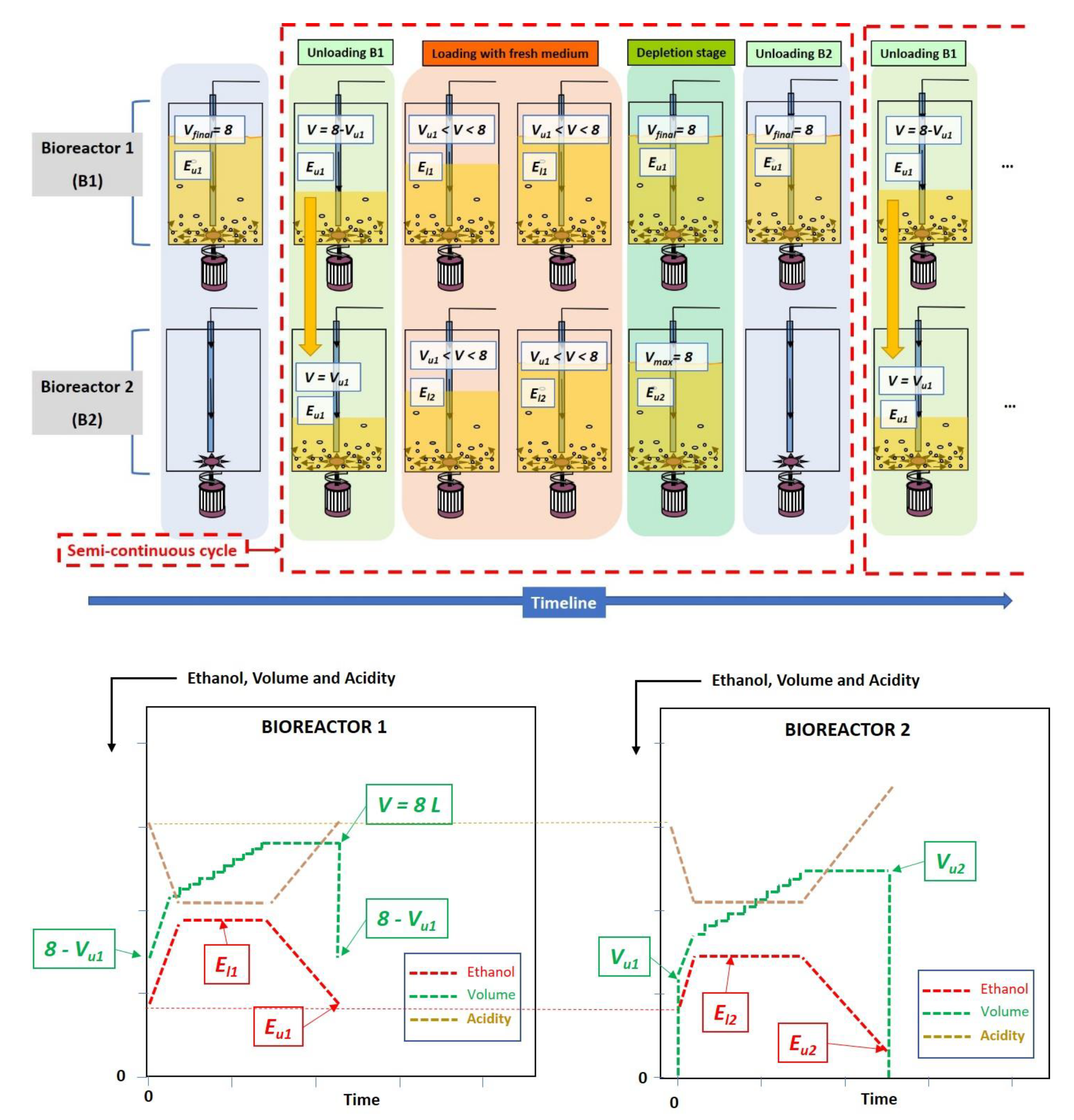
As substrate, white wine from the Montilla–Moriles D.O. (Córdoba, Spain) containing (11.5 ± 0.5) % (v/v) ethanol and an initial acidity of (0.4 ± 0.1)% (w/v) as acetic acid was used. Imitating industrial procedures, the inoculum used was a natural mixed culture [5] maintained and stored in our laboratories from experiments in a long-term fully operational bench acetator working with either wine or a synthetic ethanol medium; the original inoculum was taken, approximately a couple of years before, from an industrial tank in full operation (UNICO Vinagres y Salsas, S.L.L., Córdoba, Spain). First, a stage for reactivating and for the adaptation of the inoculum, which includes several previous acetification cycles to achieve repetitive results, was performed [27]. Additional details about some methodological aspects for obtaining the experimental data used to build the models necessary for the optimization study carried out in this work, were described elsewhere [27]; in any case, as a summary, the only variable not determined automatically was acidity, which was measured by acid—base titration with an NaOH solution approximately 0.5 N that was previously standardized with potassium hydrogen phthalate. The volume and ethanol concentration were measured in a continuous manner by using an EJA 110 differential pressure probe from Yokogawa Electric Corp. (Tokyo, Japan) and an Alkosens probe equipped with an Acetomat transducer from Heinrich Frings, respectively.

2.2. Operating Mode

Operation of the two bioreactors working serially, see Figure 2, is summarized as follows: once the ethanol concentration in the first reactor decreased to a preset value E_u1, a volume of medium V_u1 was unloaded into the second. Then, both bioreactors were loaded with fresh wine to an also preset level (E_l1 and E_l2, respectively). Once the maximum volume of medium with which each bioreactor could be loaded (8 L) was reached, the acetification system entered an ethanol depletion stage. When the ethanol concentration again fell to E_u1, the second bioreactor was completely unloaded for replenishment with medium from the first. Depending on the particular operating conditions, the second bioreactor may not be loaded to full capacity and V_u2 be less than 8 L as a result. In addition, each reactor can be operated at a different temperature (T₁ and T₂, respectively). Different values of each of the previous variables can therefore lead to minimum or maximum levels of the dependent variables.

One should bear in mind that the primary aim was to maintain the first bioreactor under non-stressing conditions for the culture to retain its activity; in this way, unloading a fraction of fermentation medium into the second bioreactor would supply it with healthy bacterial biota capable of operating under the substrate depletion conditions they would inevitably find in that reactor. By way of example, the profiles of some state variables of the system, namely, volume of medium, ethanol concentration and acetic acid concentration in each bioreactor are shown in Figure 2.

2.3. Optimization Method

The values of the operational variables providing the optimum polynomial functions were determined by solving the constrained non-linear optimization problem defined by Equation (1):

$$\begin{array}{c}Max f\left(x\right)\\ \mathrm{s}.\mathrm{t}. h\left(x\right)=0\\ g\left(x\right)\le 0\end{array},$$

(1)

where f(x) denotes the objective function, x the vector of operational (decision) variables, h(x) the set of equality constraints and g(x) that of inequality constraints.

If these functions are assumed to be differentiable, then optimal points fulfilling the Karush–Kuhn–Tucker (KKT) conditions can be determined [28,29] from the Lagrange function shown in Equation (2) for a maximization problem (for a minimization problem, the Lagrange function is the same as Equation (2) simply by changing the sign of f(x)).

$$ℒ\left(x,\lambda ,\mu \right)=f\left(x\right)-{{\displaystyle \sum }}_j^{}{\lambda }_j{h}_j\left(x\right)-{{\displaystyle \sum }}_i^{}{\mu }_i{g}_i\left(x\right),$$

(2)

where λ_j and μ_i are the KKT multipliers.

Equation (3) sets the first-order KKT conditions needed for optimality:

$$\begin{array}{c}\begin{array}{c}{\nabla }_xℒ\left(x,\lambda ,\mu \right)=0\\ h_j\left(x\right)=0\end{array}\\ \begin{array}{c}{g}_i\left(x\right)\le 0\\ {\mu }_i{g}_i\left(x\right)=0\end{array}\\ {\mu }_i\ge 0\end{array},$$

(3)

where ∇_x is the gradient operator with respect to x.

∇_xg_i and ∇_xh_j must be linearly independent of the active constraints at the critical points x* obtained as solutions to Equation (3). The active constraints at x* are those with associated non-zero KKT multipliers. In a maximization problem, if f(x) is concave and all g(x) functions are convex, then x* will be the global solution to the optimization problem. Otherwise, it will be necessary to check whether the second order KKT conditions for x* are fulfilled in order to confirm that they provide a local maximum on f(x). A function is concave if its Hessian matrix is negative semi-definite (i.e., if all its eigenvalues are equal to or less than 0) and convex if it is positive semi-definite.

Sufficient second-order KKT conditions can be verified by examining the sign of the last n − m leading principal minors of the bordered Hessian B (Equation (4)) evaluated on a critical point.

$$B\left(x,\lambda ,\mu \right)={\left(\begin{array}{cc}{\nabla }_{xx}^2ℒ\left(x,\lambda ,\mu \right)& {\nabla }_{x}g{\left(x\right)}^T\\ {\nabla }_{x}g\left(x\right)& 0_{m \times m}\end{array}\right)}_{\left(n+m\right) \times \left(n+m\right)},$$

(4)

where n is the number of operational variables, $m$ that of active constraints at the critical point, ${\nabla }_{xx}^2ℒ\left(x,\lambda ,\mu \right)$ the Hessian matrix of $ℒ\left(x,\lambda ,\mu \right)$ and g(x) the set of active constraints.

The kth leading principal minor of $B\left(x,\lambda ,\mu \right)$ equals $\left|B{\left(x,\lambda ,\mu \right)}_{k\times k}\right|$ [i.e., the determinant of the k × k submatrix taken from the upper-left of $B\left(x,\lambda ,\mu \right)$]. Therefore, the last leading principal minor of $B\left(x,\lambda ,\mu \right)$ equals $\left|B{\left(x,\lambda ,\mu \right)}_{\left(n+m\right)\times \left(n+m\right)}\right|$ [i.e., the determinant of the whole matrix $B]$, the penultimate one being $\left|B{\left(x,\lambda ,\mu \right)}_{\left(n+m-1\right)\times \left(n+m-1\right)}\right|$ and so on. For a critical point to be a local maximum, $sign\left(B{\left(x,\lambda ,\mu \right)}_{\left(n+m\right)\times \left(n+m\right)}\right)$ must be equal to (−1)ⁿ and the previous n − m − 1 leading principal minors must have an alternating sign.

3. Results and Discussion

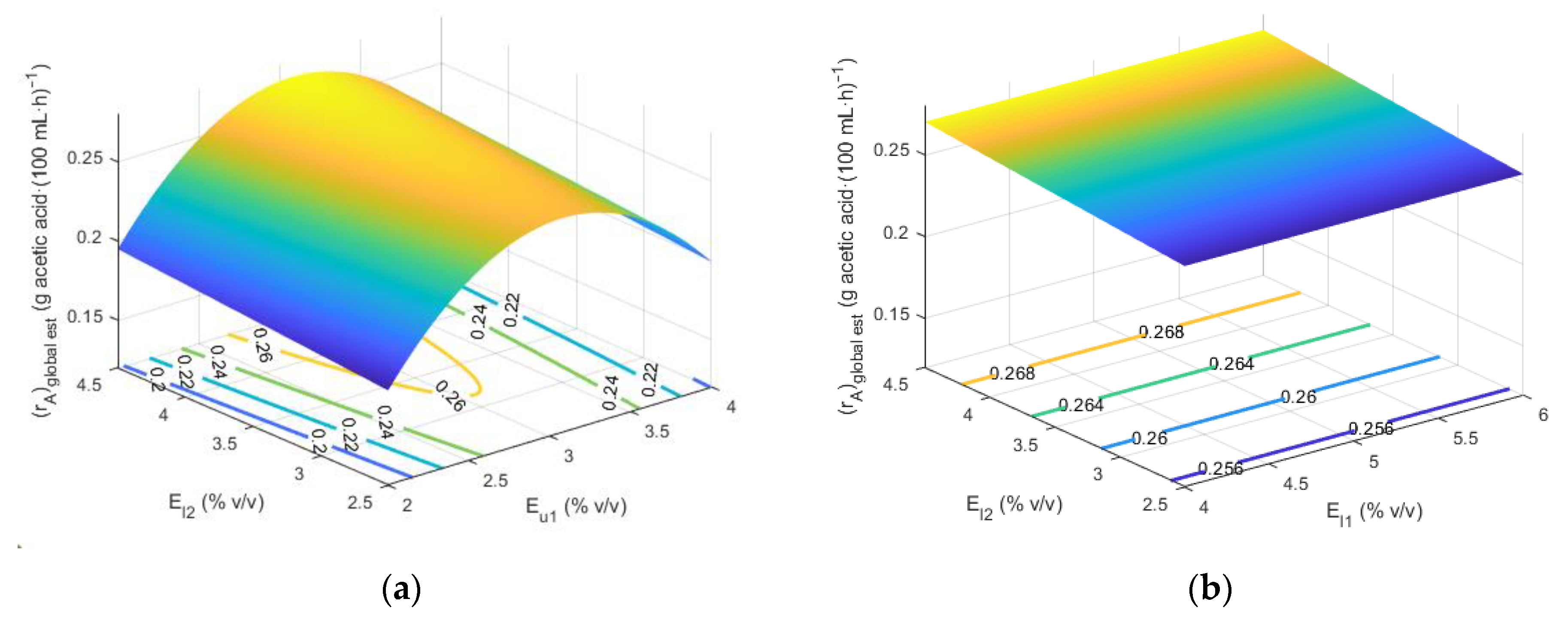
3.1. Optimization of the Mean Rate of Acetic Acid Formation in the Two-Bioreactor System

One potentially useful variable for assessing the “health” of a bioprocess and its productivity is the rate of biotransformation. Because the bioreactors operated in a non-steady state here, the target variable was the mean reaction rate, which can be estimated from the rate of ethanol consumption or that of acetic acid formation [6]. When volatile losses are negligible, as it is the case [27], both rates are identical. We focused on the mean rate of acetic acid formation, (r_A)_global, because it is easier to estimate.

In [27], the polynomial model for the mean rate of acetic acid formation in the two-bioreactor system was obtained (Equation (5)). The model allowed (r_A)_{global est} to be estimated with an error of 0.01 g acetic acid·(100 mL·h)⁻¹.

$$\begin{array}{cc}{\left(r_A\right)}_{global est}= & -0.51+0.43·E_{u1}-0.0654·E_{u1}^2\\ & -0.00456·E_{l2}·V_{u1}-0.00468·E_{u1}·E_{l1}\\ & +0.000672·T_1·E_{l1}+0.000839·E_{l2}·T_1\end{array},$$

(5)

As Equation (5) shows, not all the operational variables have a direct influence on (r_A)_{global est}; additionally, as explained in [27], particularly in its Supplementary Material (“S3.docx” file), not all the terms in Equation (5) have the same influence on (r_A)_{global est}; the higher the value of the statistic F (see

Table 1. Significance of the terms of Equation (5). (Adapted from Table S3.14 in [27], Supplementary Material (“S3.docx” file)).

Terms	F	Coefficient
Constant		−0.51
$E_{u1}^2$	342.526	−0.0654
Eu1	392.086	0.43
T1El1	56.948	0.000672
Eu1El1	28.095	−0.00468
El2T1	119.001	0.000839
El2Vu1	122.922	−0.00456

), the more significant the term is for (r_A)_{global est}; it can be seen from Table 1 that the most influential term is that of E_u1.

This model is of especial practical interest as it allows the operating conditions leading to maximum—desirable—or minimum levels of the industrially useful variables to be identified. We used the procedure described in Section 2.3 to develop a MATLAB script [30] that allowed the maximum or minimum value of (r_A)_{global est} to be calculated (see file “Optimal_rA.m” in Supplementary Materials).

The optimization problem addressed to maximize (r_A)_{global est} is represented by Equations (6) and (7). The latter sets the constraints imposed by the experimental conditions on the operational variables.

$$\begin{array}{c}\max {\left(r_A\right)}_{global est}\\ \mathrm{s}.\mathrm{t}.\end{array},$$

(6)

$$\begin{array}{c}\begin{array}{c}4.25\le V_{u1}\le 5.75\\ 4\le E_{l1}\le 6\end{array}\\ \begin{array}{c}2\le E_{u1}\le 4\\ 28\le T_1\le 32\end{array}\\ 2.5\le E_{l2}\le 4.5\end{array},$$

(7)

where V_u1 is the volume of medium unloaded from the first bioreactor into the second, E_l1 the ethanol concentration during loading of the first bioreactor, E_u1 the ethanol concentration at the time the first bioreactor is unloaded, T₁ the temperature in the first bioreactor and E_l2 the ethanol concentration in the second bioreactor during loading.

Solving the previous optimization problem provided the operating conditions of

Table 2. Values of the operational variables needed to maximize (r_A)_{global est}.

Vu1, L	El1, % (v/v)	Eu1, % (v/v)	T1, °C	El2, % (v/v)	T2, °C	(rA)global est, g Acetic Acid·(100 mL·h)−1
4.25	6.0	3.07	32.0	4.5	–	0.27

.

Because of the number of involved operational variables, it is not straightforward to graphically show the optimum obtained with the conditions of Table 2. Nevertheless, considering the previous comments on the significance of the terms in Equation (5), when plotting the response surfaces of (r_A)_{global est} varying just a pair of the operational variables at once, it is possible to show that significant changes can only be found when the variable E_u1 is included. By way of example, response surfaces varying E_u1 and E_l2 on one side and E_l1 and E_l2 on the other are shown in Figure 3a,b, respectively. Values from Table 2 are used for the remaining variables.

Since (r_A)_{global est} could be subject to an error of up to 0.01 g acetic acid·(100 mL·h)⁻¹, we checked whether other combinations of values of the operational variables falling within the ranges imposed by their errors would lead to maximum values over the range 0.26 ≤ (r_A)_{global est} ≤ 0.27 g acetic acid·(100 mL·h)⁻¹. A systematic analysis provided the ranges shown in

Table 3. Upper and lower end of the ranges over which the operational variables maximized (r_A)_{global est}.

End	Vu1, L	El1, % (v/v)	Eu1, % (v/v)	T1, °C	El2, % (v/v)	T1, °C
Lower ↕ Upper	4.25 ↕ 4.50	5.6 ↕ 6.0	2.8 ↕ 3.2	31.6 ↕ 32.0	4.1 ↕ 4.5	–

. With a 0.2 interval for each variable, such ranges led to a total of 162 combinations of which only 109 (see Table S1 in file “S1.docx” in Supplementary Materials) fell within the previous range of (r_A)_{global est}. However, using all 162 combinations ensured that this variable would be very close to its maximum value: 0.25–0.27 g acetic acid·(100 mL·h)⁻¹. Therefore, any of the 162 combinations would, in theory, lead to the highest possible mean rate of acetic acid formation in the two-bioreactor system—and hence to values of each operational variable falling in the ranges of Table 3.

Conversely, minimizing (r_A)_{global est} led to the results of

Table 4. Values of the operational variables needed to minimize (r_A)_{global est}.

Vu1, L	El1, % (v/v)	Eu1, % (v/v)	T1, °C	El1, % (v/v)	T2, °C	(rA)global est, g Acetic Acid·(100 mL·h)−1
5.75	4.0	2.0	28	4.5	–	0.11

(see file “Optimal_rA.m” in Supplementary Materials). The problem was like that stated in Equations (6) and (7) except that the aim was to minimize (r_A)_{global est} rather than maximize it.

As in the previous case, the error made in modelling (r_A)_{global est} was used to examine the combinations of values of the operational variables, with provision for their errors (see

Table 5. Upper and lower end of the ranges over which the operational variables minimized (r_A)_{global est}.

End	Vu1, L	El1, % (v/v)	Eu1, % (v/v)	T1, °C	El1, % (v/v)	T2, °C
Lower ↕ Upper	5.45 ↕ 5.75	4.0 ↕ 4.8	2.0	28.0 ↕ 28.8	2.5 ↕ 4.5	–

), leading to minimum values over the range 0.11 ≤ (r_A)_{global est} ≤ 0.12 g acetic acid·(100 mL·h)⁻¹. The ranges of Table 5 for the operational variables, with 0.2 unit intervals, led to a total of 550 combinations only 29 of which provided an (r_A)_{global est} value falling in the previous range of minimum values (see Table S2 in file “S1.docx” in Supplementary Materials). However, any of the 550 combinations ensured that (r_A)_{global est} would fall in the range 0.116–0.135 g acetic acid·(100 mL·h)⁻¹ and thus be very close to the minimum of Table 4. Therefore, any combination would provide the lowest mean rate of acetic acid formation in the two-bioreactor system and lead to values of the operational variables falling in the ranges of Table 5.

Applying the equations obtained in [27] to the other variables (Equations (8)–(16)) provided the estimated values of

Table 6. Values of the state variables under the operating conditions maximizing and minimizing (r_A)_{global est}.

Variable	Conditions Minimizing (rA)global est (0.11 g Acetic Acid·(100 mL·h)−1)	Conditions Maximizing (rA)global est (0.27 g Acetic Acid·(100 mL·h)−1)
Pm est, g acetic acid·h−1	20.6 ± 0.7 ↔ 22.0 ± 0.7	27.5 ± 0.7 ↔ 28.6 ± 0.7
Eu2 est, % (v/v)	0 ± 0.3 ↔ 0.4 ± 0.3	1.4 ± 0.3 ↔ 2.2 ± 0.3
Vu2 est, L	7.77 ± 0.22 ↔ 7.99 ± 0.22	7.63 ± 0.22 ↔ 7.97 ± 0.22
tcycle est, h	51.1 ± 2.5	20.8 ± 2.5
Vm est, L	14.04 ± 0.33 ↔ 14.32 ± 0.33	14.06 ± 0.33 ↔ 14.36 ± 0.33
EtOHm1 est, % (v/v)	3.8 ± 0.2	5.2 ± 0.2
EtOHm2 est, % (v/v)	2.4 ± 0.4 ↔ 2.7 ± 0.4	3.6 ± 0.4 ↔ 3.9 ± 0.4
HAcm1 est, % (w/v)	7.7 ± 0.2	6.3 ± 0.2
HAcm2 est, % (w/v)	8.8 ± 0.4 ↔ 9.1 ± 0.4	7.5 ± 0.4 ↔ 7.9 ± 0.4

for P_{m est}, E_{u2 est}, V_{u2 est}, t_{cycle est}, V_{m est}, EtOH_{m1 est}, EtOH_{m2 est}, HAc_{m1 est} and HAc_{m2 est} under the operating conditions maximizing or minimizing (r_A)_{global est}. The ranges of some variables reflect differences due to the influence of T₂ —like (r_A)_{global est}, other variables were independent of the temperature in the second reactor, however.

$$\begin{array}{cc}{P}_{m est}=& -243.705+18.324·V_{u1}+72.736·E_{l1}+21.525·E_{u1}\\ & -9.708·E_{l1}^2-1.102·E_{u1}·V_{u1}-0.534·T_1·V_{u1}\\ & \begin{array}{c}+0.742·T_1·E_{l1}-0.416·E_{l2}·E_{l1}+0.175·T_2·E_{l1}\\ -0.12·T_1·E_{u1}-0.399·T_2·E_{u1}+0.101·T_2·E_{l2}\end{array}\end{array},$$

(8)

$$\begin{array}{cc}{E}_{u2 est} =& 14.935-5.371·E_{u1}+0.988·E_{u1}^2-0.0592·E_{l1}·V_{u1}\\ & -0.456·E_{u1}·V_{u1}+0.0678·E_{u1}·E_{l1}\\ & +0.494·E_{l2}·E_{u1}-0.049·T_2·E_{l2}\end{array},$$

(9)

$$\begin{array}{cc}{V}_{u2 est}= & 4.921+1.399·E_{l2}-0.59·E_{u1}^2\\ & +0.665·E_{u1}·V_{u1}-0.324·E_{l2}·V_{u1}\\ & +0.172·E_{l2}·E_{u1}-0.0275·T_2·E_{u1}\end{array},$$

(10)

$$\begin{array}{cc}{t}_{cycle est} =& 518.591-156.652·V_{u1}\\ & -6.474·T_1+13.556·V_{u1}^2\\ & +1.076·T_1·V_{u1}-0.864·E_{u1}·E_{l1}\end{array},$$

(11)

$$\begin{array}{cc}{V}_{m est}=& 4.306+4.739·E_{u1}-0.841·E_{u1}^2\\ & \begin{array}{c}+0.336·E_{u1}·V_{u1}-0.0127·T_2·V_{u1}\\ -0.125·E_{l2}·E_{l1}+0.0326·T_2·E_{l1}\\ -0.0735·T_2·E_{u1}+0.0358·T_2·E_{l2}\end{array}\end{array},$$

(12)

$$\begin{array}{cc}EtO{H}_{m1 est}=& 2.312-0.0932·E_{u1}^2\\ & +0.0191·E_{l1}·V_{u1}+0.175·E_{u1}·E_{l1}\end{array},$$

(13)

$$\begin{array}{cc}EtO{H}_{m2 est}=& 4.327-0.179·E_{u1}·V_{u1}\\ & +0.306·E_{l2}·E_{u1}-0.0182·T_2·E_{l2}\end{array},$$

(14)

$$\begin{array}{cc}HA{c}_{m1 est}=& 9.188+0.0932·E_{u1}^2\\ & -0.0191·E_{l1}·V_{u1}-0.175·E_{u1}·E_{l1}\end{array},$$

(15)

$$\begin{array}{cc}HA{c}_{m2 est}=& 7.227+0.177·E_{u1}·V_{u1}\\ & -0.305·E_{l2}·E_{u1}+0.0178·T_2·E_{l2}\end{array},$$

(16)

Based on the previous results, the highest and lowest mean rate of acetic acid production were obtained by using extreme values of some operational variables. Thus, the minimum (r_A)_{global est} value (Table 4) was obtained with the lowest temperature in the first bioreactor (T₁ = 28 °C), and the smallest values in the ranges of E_l1 and E_u1 [viz., 4% and 2% (v/v), respectively]. These results suggest that the smaller the amount of substrate available to AAB and the higher the acidity to which the bacteria are exposed during a fermentation cycle (see EtOH_{m1 est} and HAc_{m1 est} values in Table 6) are, the less suitable will be the medium for their metabolic action —and hence for acetification. Also, because the volume of medium unloaded from the first bioreactor was quite substantial (V_u1 = 5.75 L), the amount of inoculum remaining in it for the next cycle was considerably reduced, and so was (r_A)_{global est} as a consequence. This result is consistent with those of modelling studies on a single bioreactor using both first-principles and black-box models [8,9,10,22,23,31,32].

On the other hand, if the aim is to maximize (r_A)_{global est}, the operating conditions should be essentially the opposite of those described in the previous paragraph. As can be seen from Table 6, such conditions resulted in increased mean substrate availability and decreased mean acidity in both bioreactors.

One other interesting conclusion is that P_{m est} is rather different under the conditions maximizing and minimizing (r_A)_{global est} (see Table 6). As expected, the greater (r_A)_{global est} is, the higher will be acetic acid production. However, as shown in the following section, the maximum mean rate did not result in the highest possible P_{m est} level.

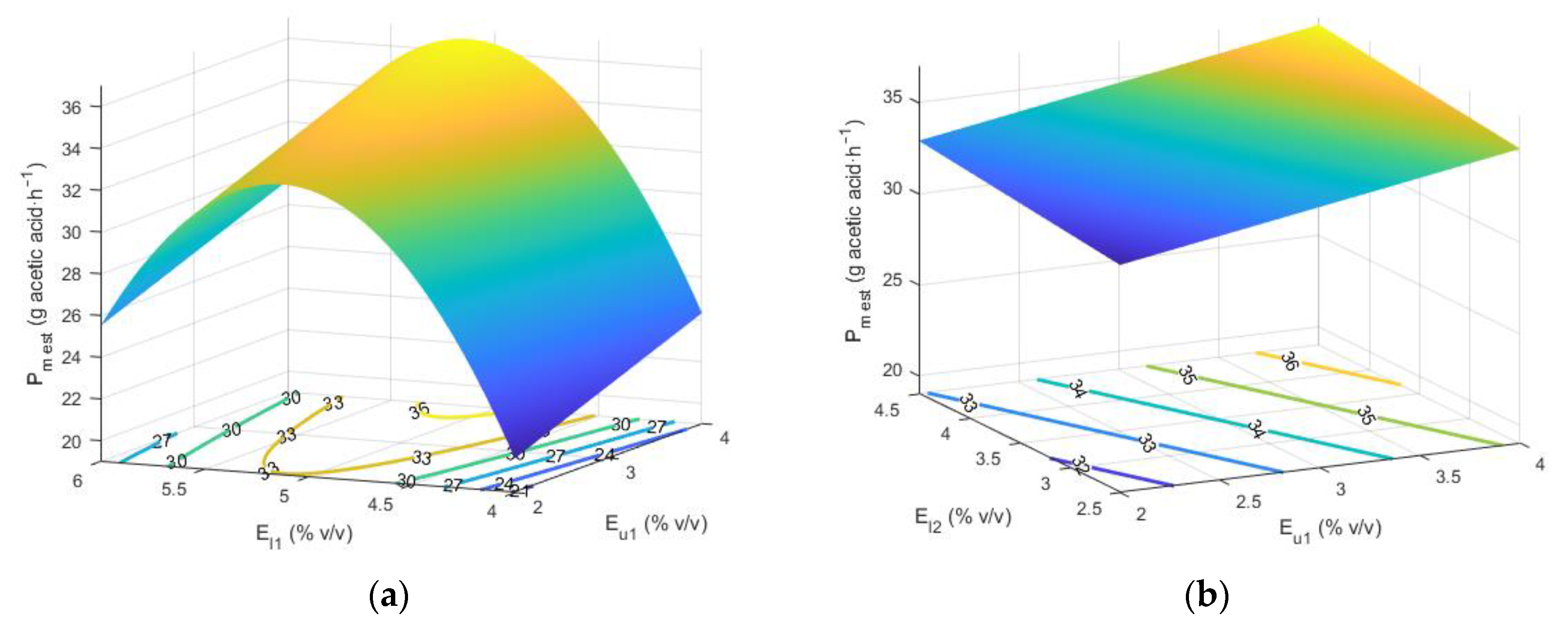
3.2. Optimization of P_{m est}

The variable (r_A)_{global est} possesses a high industrial interest. In practice, however, the aim of a vinegar producing plant is to obtain as much acetic acid per hour of operation (i.e., to maximize the overall production of acid, P_m). This variable can be estimated with an error of 0.7 g acetic acid·h⁻¹ from Equation (8). In this Equation, only three of the operational variables (E_l1, E_u1 and V_u1) have a direct influence on P_{m est}, but as explained before in the case of Equation (5), not all the terms in Equation (8) have the same influence on P_{m est} (see

Table 7. Significance of the terms of Equation (8). (Adapted from Table S3.27 in [27], Supplementary Material (“S3.docx” file)).

Terms	F	Coefficient
Constant		−243.705
T1El1	92.918	0.742
$E_{l1}^2$	961.793	−9.708
El1	326.099	72.736
T2El2	34.06	0.101
T1Vu1	58.929	−0.534
Vu1	46.188	18.324
Eu1	63.689	21.525
T2Eu1	77.65	−0.399
T2El1	35.845	0.175
El2El1	16.55	−0.416
Eu1Vu1	19.078	−1.102
T1Eu1	5.284	−0.12

); the higher the value of the statistic F, the more significant the term is for P_{m est}; it can be seen from Table 7 that the most influential term is that of E_l1.

Below is described the procedure followed to identify the operating conditions maximizing (the industrial target) or minimizing (an undesirable outcome) P_{m est}.

The procedure of Section 2.3 to develop a MATLAB script to identify the optimum (maximum or minimum) P_{m est} value was used (see file “Optimal_Prod.m” in Supplementary Materials). The conditions maximizing P_{m est} can be identified by solving Equations (17) and (18), the latter containing the constraints imposed by the values of the experimental variables under the experimental conditions used.

$$\begin{array}{c}\max P_{m est}\\ \mathrm{s}.\mathrm{t}.\end{array},$$

(17)

$$\begin{array}{c}\begin{array}{c}4.25\le V_{u1}\le 5.75\\ 4\le E_{l1}\le 6\end{array}\\ \begin{array}{c}2\le E_{u1}\le 4\\ 28\le T_1\le 32\end{array}\\ \begin{array}{c}2.5\le E_{l2}\le 4.5\\ 28\le T_2\le 32\end{array}\end{array},$$

(18)

where T₂ is the temperature in the second bioreactor.

Table 8. Values of the operational variables needed to maximize P_{m est}.

Vu1, L	El1, % (v/v)	Eu1, % (v/v)	T1, °C	El2, % (v/v)	T2, °C	Pm est, g Acetic Acid·h−1
4.25	5.1	4.0	32	4.5	28	36.6

shows the value of each operational variable maximizing P_{m est} and hence the solution to the optimization problem.

In a similar way to the previous discussion on (r_A)_{global est}, plotting the response surfaces of P_{m est} varying just a pair of the operational variables at once, it is possible to show that significant changes can only be found when the variable E_l1 is included. By way of example, response surfaces varying E_l1 and E_u1 on one side and E_u1 and E_l2 on the other are shown in Figure 4a,b, respectively. Values from Table 8 are used for the remaining variables.

Similarly to (r_A)_{global est}, the errors in P_{m est} and the operational variables were used to identify the combinations of variables leading to values over the range 35.9 ≤ P_{m est} ≤ 36.6 g acetic acid·h⁻¹ (see

Table 9. Upper and lower end of the ranges over which the operational variables maximized P_{m est}.

End	Vu1, L	El1, % (v/v)	Eu1, % (v/v)	T1, °C	El2, % (v/v)	T2, °C
Lower	4.25	4.9	3.7	31.3	3.5	28.0
↕	↕	↕	↕	↕	↕	↕
Upper	4.45	5.3	4.0	32.0	4.5	30.9

). The ranges of Table 9, at 0.2 unit intervals, allowed a total of 4320 combinations to be identified of which 50 provided a P_{m est} value within the previous range (see Table S3 in file “S1.docx” in Supplementary Materials). However, any of the 4320 combinations led to a very high P_{m est} value (32.8–36.6 g acetic acid·h⁻¹, which are close to that range). Therefore, any of the combinations of operational variables at values within the ranges of Table 9 would lead to a near-maximum P_{m est} value.

Minimizing P_{m est} provided the results of

Table 10. Values of the operational variables needed to minimize P_{m est}.

Vu1, L	El1, % (v/v)	Eu1, % (v/v)	T1, °C	El2, % (v/v)	T2, °C	Pm est, g Acetic Acid·h−1
5.75	4.0	4.0	31.9	2.5	32	14.7

(see file “Optimal_Prod.m” in Supplementary Materials).

The combinations of values of the operational variables leading to minimum P_{m est} values over the range 14.7 ≤ P_{m est} ≤ 15.4 g acetic acid·h⁻¹ were identified similarly to those maximizing this dependent variable. Using the values in the ranges of

Table 11. Upper and lower end of the ranges over which the operational variables minimized P_{m est}.

End	Vu1, L	El1, % (v/v)	Eu1, % (v/v)	T1, °C	El2, % (v/v)	T2, °C
Lower ↕ Upper	5.55 ↕ 5.75	4.0	3.6 ↕ 4.0	31.2 ↕ 32.0	2.5 ↕ 2.9	31.3 ↕ 32.0

(0.2 unit intervals) provided 360 combinations of which 36 leading to P_{m est} values within the previous range (see Table S4 in file “S1.docx” in Supplementary Materials). However, all combinations led to very low P_{m est} values: 14.6–17.1 g acetic acid·h⁻¹, which are very close to the minimum value.

Table 12. Values of the state variables under the operating conditions maximizing and minimizing P_{m est}.

Variable	Conditions Minimizing Pm est (14.7 g Acetic Acid·h−1)	Conditions Maximizing Pm est (36.6 g Acetic Acid·h−1)
(rA)global est, g acetic acid·(100 mL·h)−1	0.18 ± 0.01	0.21 ± 0.01
Eu2 est, % (v/v)	0.0 ± 0.3	4.3 ± 0.3
Vu2 est, L	7.56 ± 0.22	6.71 ± 0.22
tcycle est, h	43.0 ± 2.5	19.2 ± 2.5
Vm est, L	11.58 ± 0.33	12.07 ±0.33
EtOHm1 est, % (v/v)	4.1 ± 0.2	4.8 ± 0.2
EtOHm2 est, % (v/v)	1.8 ± 0.4	4.5 ± 0.4
HAcm1 est, % (w/v)	7.4 ± 0.2	6.7 ± 0.2
HAcm2 est, % (w/v)	9.7 ± 0.4	7.0 ±0.4

compares the values of the estimated state variables for the maximum and minimum P_{m est} values.

As can be seen, the conditions maximizing P_{m est} were different from those maximizing (r_A)_{global est}. In fact, P_{m est} and (r_A)_{global est} are related by the mean volume of medium, V_{m est}, in Equation (19). Since the bioreactors worked in a semi-continuous mode, the mean volume was dependent on the particular operating conditions and those resulting in the maximum possible values of P_{m est} and (r_A)_{global est} need not coincide (see V_{m est} values in Table 6 and Table 12).

$${\left(r_A\right)}_{global est}=\frac{P_{m est}}{V_{m est}},$$

(19)

As stated above for (r_A)_{global est}, an increased mean availability of ethanol and a decreased mean acidity boosted acetic acid production (P_m). However, ethanol and acetic acid concentrations above certain levels have an inhibitory effect whereas too low levels can even boost bacterial activity. These effects have been extensively examined in modelling studies [8,9,10,22,23,31,32]. For example, ethanol concentrations above 6% (v/v) and acetic acid concentrations above 6% (w/v) have been found to have substantial inhibitory effects [8,9,10]. This knowledge, and the mean acidity and ethanol values of Table 6 and Table 12, allow the (r_A)_{global est} and P_{m est} results to be more easily understood.

One other major inference is that, based on Table 12, maximizing P_{m est} leaves a substantial amount of unavailable ethanol in the second bioreactor [E_u2 = 4.3% (v/v)], which is, in general, industrially unacceptable. It is, therefore, interesting to identify the specific conditions that will maximize P_{m est} while ensuring that the substrate is depleted to an acceptable degree. The procedure followed for this purpose is described in the following section.

3.3. Optimizing P_{m est} While Ensuring Enough Substrate Depletion

For economy and legal reasons, the amount of ethanol present in industrially produced vinegar must not exceed prescribed levels depending on each specific type of vinegar. It is therefore important to identify the operating conditions optimizing acetic acid production (P_{m est} in Equation (8)) under a constraint on the ethanol concentration at the time the second bioreactor is unloaded (E_{u2 est} in Equation (9)). The optimization problem is stated in Equations (20) and (21).

$$\begin{array}{c}\max P_{m est}\\ \mathrm{s}.\mathrm{t}.\end{array},$$

(20)

$$\begin{array}{c}\begin{array}{c}4.25\le V_{u1}\le 5.75\\ 4\le E_{l1}\le 6\end{array}\\ \begin{array}{c}2\le E_{u1}\le 4\\ 28\le T_1\le 32\end{array}\\ \begin{array}{c}2.5\le E_{l2}\le 4.5\\ \begin{array}{c}28\le T_2\le 32\\ E_{u2 est}=constant\end{array}\end{array}\end{array},$$

(21)

where constant is the ethanol concentration at unloading time in the second reactor to be imposed.

Table 13. Values of the operational variables needed to maximize P_{m est} with an E_{u2 est} value of 0.2%, 0.5%, 1.0% or 1.5% (v/v).

Vu1, L	El1, % (v/v)	Eu1, % (v/v)	T1, °C	El2, % (v/v)	T2, °C	Pm est, g Acetic Acid·h−1	Eu2 est, % (v/v)
4.76	5.2	2.3	32.0	4.5	32.0	34.6	0.2
4.53	5.2	2.4	32.0	4.5	32.0	34.9	0.5
4.25	5.2	2.7	32.0	4.5	32.0	35.4	1.0
4.25	5.2	3.2	32.0	4.5	32.0	35.5	1.5

shows the values of the operational variables providing the solution to the previous problem with E_{u2 est} values from 0.2% to 1.5% (v/v).

The solution was obtained by using the MATLAB script of Section 3.2 (see file “Optimal_Prod.m” in Supplementary Materials) as expanded with the constraint on E_{u2 est}. The previous range of E_{u2 est} was used to consider virtually complete and less marked depletion of the substrate because some vinegars (particularly those under a designation of origin or aged in casks) are allowed to contain higher levels of residual ethanol.

As expected, the greater E_{u2 est} was (i.e., the less markedly the substrate was depleted in the second bioreactor), the more favored was AAB activity and the higher was acetic acid productivity as a result.

3.4. Comparison of the Performance of Serial and Parallel Bioreactors

This was one other point of especial interest. For this purpose, we compared the results obtained with the two bioreactors working in series here and those previously reported for others operating in parallel [8,9,10,22,23,31,32]. Because the previous studies were conducted at 31 °C, we estimated P_m and E_u2 at that temperature. As can be seen from

Table 14. Comparison of acetic acid production and final ethanol concentration at the time of unloading with two bioreactors operating in series and in parallel.

	Optimizing Production			Optimizing Production with a Specific Final Eu2 Value
Working mode	Parallel (31 °C)	Series		Parallel (31 °C)	Series
		T1 = 31 °C T2 = 31 °C	T1 = 32 °C T2 = 28 °C		T1 = 31 °C T2 = 31 °C	T1 = 32 °C T2 = 32 °C
Pm g acetic acid·h−1	35.2 ± 0.5	34.8 ± 0.7	35.9 ± 0.7	29.6 ± 0.5	33.2 ± 0.7	34.2 ± 0.7
Eu2 % (v/v)	3.0 ± 0.2	3.7 ± 0.3	4.3 ± 0.3	0.5 ± 0.2	0.5 ± 0.3	0.5 ± 0.3

, there were no substantial differences in performance between the serial and parallel configurations when P_m was maximized under no constraint on E_u2—not even at the optimum T₁ and T₂ values found here. However, maximizing P_m with E_u2 = 0.5% (v/v) resulted in the serial system being more productive than the parallel one. Specifically, at 31 °C the former system reached a P_m 12.2% higher than did the latter. It was impossible to directly compare productivity with the two systems at 32 °C and E_u2 = 0.5% (v/v) because no productivity data for the parallel system at that temperature were available. In any case, the results of Table 14 suggest that they cannot be too different from those obtained at 31 °C.

Finally, it should be noted that using two serial bioreactors results in very high acetic acid productivity and virtually complete depletion of ethanol. On the other hand, as shown in a previous work [16], depleting the second bioreactor in a system operating in parallel would slow down the process as a result of the time needed for acetic acid bacteria to regain full activity after a period of substrate scarcity and a high acidity in the medium—all of which considerably detract from productivity [16].

4. Conclusions

The two serially arranged bioreactors system for the acetification process has been optimized in various respects using previous quadratic polynomial models. The values of the operational variables maximizing or minimizing the mean rate of acetic acid production were obtained: a maximum value of (r_A)_{global est}= 0.27 g acetic acid·(100 mL·h)⁻¹ was achieved when V_u1 = 4.25 L, E_l1 = 6% (v/v), E_u1 = 3.07% (v/v), T₁ = 32 °C, E_l2 = 4.5% (v/v) and a minimum value of (r_A)_{global est} = 0.11 g acetic acid·(100 mL·h)⁻¹ was achieved when V_u1 = 5.75 L, E_l1 = 4% (v/v), E_u1 = 2% (v/v), T₁ = 28 °C, E_l2 = 4.5% (v/v).

In addition, the conditions leading to the maximum and minimum productivity were: P_{m est} = 36.6 g acetic acid·h⁻¹ was achieved when V_u1 = 4.25 L, E_l1 = 5.1% (v/v), E_u1 = 4% (v/v), T₁ = 32 °C, E_l2 = 4.5% (v/v), T₂ = 28 °C and P_{m est} = 14.7 g acetic acid·h⁻¹ was achieved when V_u1 = 5.75 L, E_l1 = 4% (v/v), E_u1 = 4% (v/v), T₁ = 31.9 °C, E_l2 = 2.5% (v/v), T₂ = 32 °C.

The operating conditions needed to maximize productivity while ensuring ethanol depletion to a preset degree were also identified: 4.25 ≤ V_u1 ≤ 4.76 L, E_l1 = 5.2% (v/v), 2.3 ≤ E_u1 ≤ 3.2% (v/v), T₁ = 32 °C, E_l2 = 4.5% (v/v), T₂ = 32 °C to achieve 34.6 ≤ P_m ≤ 35.5 g acetic acid·h⁻¹ with 0.2 ≤ E_u2 ≤ 1.5% (v/v). Such conditions allowed near-maximum productivity to be obtained.

One other aim fulfilled by modelling the system and using results of previous research work was to compare the performance of the system with the two reactors operating in series and in parallel. P_m can be maximized with no restrictions on E_u2 by using either configuration. However, if the substrate is to be depleted [e.g., E_u2 = 0.5% (v/v)], then the serial configuration will be more productive.

References

1. Rončević, Z.; Grahovac, J.; Dodić, S.; Vučurović, D.; Dodić, J. Utilisation of winery wastewater for xanthan production in stirred tank bioreactor: Bioprocess modelling and optimisation. Food Bioprod. Process. 2019, 117, 113–125. [Google Scholar] [CrossRef]
2. El-Naggar, N.E.A.; Haroun, S.A.; El-Weshy, E.M.; Metwally, E.A.; Sherief, A.A. Mathematical modeling for bioprocess optimization of a protein drug, uricase, production by Aspergillus welwitschiae strain 1–4. Sci. Rep. 2019, 9, 12971. [Google Scholar] [CrossRef] [PubMed]
3. Beagan, N.; O’Connor, K.E.; Del Val, I.J. Model-based operational optimisation of a microbial bioprocess converting terephthalic acid to biomass. Biochem. Eng. J. 2020, 158, 107576. [Google Scholar] [CrossRef]
4. Adeetunji, A.I.; Olaniran, A.O. Statistical modelling and optimization of protease production by an autochthonous Bacillus aryabhattai Ab15-ES: A response surface methodology approach. Biocatal. Agric. Biotechnol. 2020, 24, 101528. [Google Scholar] [CrossRef]
5. Román-Camacho, J.J.; Santos-Dueñas, I.M.; García-García, I.; Moreno-García, J.; García-Martínez, T.; Mauricio, J.C. Metaproteomics of microbiota involved in submerged culture production of alcohol wine vinegar: A first approach. Int. J. Food Microbiol. 2020, 333, 108797. [Google Scholar] [CrossRef] [PubMed]
6. García-García, I.; Cantero-Moreno, D.; Jiménez-Ot, C.; Baena-Ruano, S.; Jiménez-Hornero, J.; Santos-Duenas, I.; Bonilla-Venceslada, J.L.; Barja, F. Estimating the mean acetification rate via on-line monitored changes in ethanol during a semi-continuous vinegar production cycle. J. Food Eng. 2007, 80, 460–464. [Google Scholar] [CrossRef]
7. García-García, I.; Jiménez-Hornero, J.E.; Santos-Dueñas, I.M.; González-Granados, Z.; Cañete-Rodríguez, A.M. Modelling and optimization of acetic acid fermentation (Chapter 15). In Advances in Vinegar Production; Bekatorou, A., Ed.; CRC Press (Taylor & Francis Group): Boca Raton, FL, USA, 2019; pp. 299–325. [Google Scholar] [CrossRef]
8. Jiménez-Hornero, J.E.; Santos-Dueñas, I.M.; García-García, I. Optimization of biotechnological processes. The acetic acid fermentation. Part I: The proposed model. Biochem. Eng. J. 2009, 45, 1–6. [Google Scholar] [CrossRef]
9. Jiménez-Hornero, J.E.; Santos-Dueñas, I.M.; Garcia-Garcia, I. Optimization of biotechnological processes. The acetic acid fermentation. Part II: Practical identifiability analysis and parameter estimation. Biochem. Eng. J. 2009, 45, 7–21. [Google Scholar] [CrossRef]
10. Jiménez-Hornero, J.E.; Santos-Dueñas, I.M.; Garcia-Garcia, I. Optimization of biotechnological processes. The acetic acid fermentation. Part III: Dynamic optimization. Biochem. Eng. J. 2009, 45, 22–29. [Google Scholar] [CrossRef]
11. Jiménez-Hornero, J.E.; Santos-Dueñas, I.M.; García-García, I. Modelling acetification with artificial neural networks and comparison with alternative procedures. Processes 2020, 8, 749. [Google Scholar] [CrossRef]
12. García-García, I.; Santos-Dueñas, I.M.; Jiménez-Ot, C.; Jiménez-Hornero, J.E.; Bonilla-Venceslada, J.L. Vinegar engineering. In Vinegars of the World; Solieri, L., Giudici, P., Eds.; Springer: Milano, Italy, 2009; Chapter 9; pp. 97–120. [Google Scholar] [CrossRef]
13. Jiménez-Ot, C.; Santos-Dueñas, I.M.; Jiménez-Hornero, J.; Baena-Ruano, S.; Martín-Santos, M.A.; Bonilla-Venceslada, J.L.; García-García, I. Influencia de la graduación total de un vino Montilla-Moriles sobre la velocidad de acetificación en el proceso de elaboración de vinagre. In XVI Congreso Nacional de Microbiología de los Alimentos, Córdoba, Spain; Fernández-Salguero, J., García-Jimeno, R., Medina-Canalejo, L., Cabezas Redondo, L., Eds.; Publication Services of Diputación de Córdoba: Córdoba, Spain, 2008; pp. 255–256. [Google Scholar]
14. Baena-Ruano, S.; Jiménez-Ot, C.; Santos-Dueñas, I.M.; Cantero-Moreno, D.; Barja, F.; García-García, I. Rapid method for total, viable and non-viable acetic acid bacteria determination during acetification process. Process Biochem. 2006, 41, 1160–1164. [Google Scholar] [CrossRef]
15. Baena-Ruano, S.; Jiménez-Ot, C.; Jiménez-Hornero, J.; Santos-Dueñas, I.M.; Bonilla-Venceslada, J.L.; Cantero-Moreno, D.; García-García, I. In Proceedings of the Second Symposium on Research+Development+Innovation for Vinegars Production, Córdoba, Spain, 26–28 April 2006; García-García, I., Ed.; University of Córdoba: Córdoba, Spain, 2006; pp. 180–183. [Google Scholar]
16. Baena-Ruano, S.; Jiménez-Ot, C.; Santos-Dueñas, I.M.; Jiménez-Hornero, J.E.; Bonilla-Venceslada, J.L.; Álvarez-Cáliz, C.; García-García, I. Influence of the final ethanol concentration on the acetification and production rate in the wine vinegar process. J. Chem. Technol. Biotechnol. 2010, 85, 908–912. [Google Scholar] [CrossRef]
17. Álvarez-Cáliz, C.; Santos-Dueñas, I.M.; Cañete-Rodríguez, A.M.; García-Martínez, T.; Maurico, J.C.; García-García, I. Free amino acids, urea and ammonium ion contents for submerged wine vinegar production: Influence of loading rate and air-flow rate. Acetic Acid Bact. 2012, 1, e1. [Google Scholar] [CrossRef]
18. Emde, F. State of the art technologies in submersible vinegar production. In Proceedings of the Second Symposium on Research+Development+Innovation for Vinegars Production, Córdoba, Spain, 26–28 April 2006; García-García, I., Ed.; University of Córdoba: Córdoba, Spain, 2006; pp. 101–109. [Google Scholar]
19. Sellmer, S. New strategies in process control for the production of wine vinegar. In Proceedings of the Second Symposium on Research+Development+Innovation for Vinegars Production, Córdoba, Spain, 26–28 April 2006; García-García, I., Ed.; University of Córdoba: Córdoba, Spain, 2006; pp. 127–132. [Google Scholar]
20. González-Sáiz, J.M.; Pizarro, C.; Garrido-Vidal, D. Evaluation of kinetic models for industrial acetic fermentation: Proposal of a new model optimized by genetic algorithms. Biotechnol. Prog. 2003, 19, 599–611. [Google Scholar] [CrossRef] [PubMed]
21. Garrido-Vidal, D.; Pizarro, C.; Gonzalez-Saiz, J.M. Study of process variables in industrial acetic fermentation by a continuous pilot fermentor and response surfaces. Biotechnol. Prog. 2003, 19, 1468–1479. [Google Scholar] [CrossRef] [PubMed]
22. Jiménez-Hornero, J.E.; Santos-Dueñas, I.M.; Garcia-Garcia, I. Structural identifiability of a model for the acetic acid fermentation process. Math. Biosci. 2008, 216, 154–162. [Google Scholar] [CrossRef] [PubMed]
23. Santos-Dueñas, I.M.; Jimenez-Hornero, J.E.; Cañete-Rodríguez, A.M.; García-García, I. Modeling and optimization of acetic acid fermentation: A polynomial-based approach. Biochem. Eng. J. 2015, 99, 35–43. [Google Scholar] [CrossRef]
24. Nguyen, N.K.; Borkowski, J.J. New 3-level response surface designs constructed from incomplete block designs. J. Stat. Plan Inference 2008, 138, 294–305. [Google Scholar] [CrossRef]
25. Abilov, A.G.; Aliev, V.S.; Rustamov, M.I.; Aliev, N.M.; Lutfaliev, K.A. Problems of control and chemical engineering experiment, Part 1 1D: 45. In Proceedings of the IFAC 6th Triennal World Congress, Boston/Cambridge, MA, USA, 24–30 August 1975; pp. 1–7. [Google Scholar]
26. Box, G.E.P.; Hunter, J.S.; Hunter, W.G. Statistics for Experimenters: Design, Innovation and Discovery, 2nd ed.; John Wiley & Sons, Inc.: Hoboken, NJ, USA, 2008; pp. 1–672. ISBN 978-0-471-71813-0. [Google Scholar]
27. Álvarez-Cáliz, C.; Santos-Dueñas, I.M.; Jiménez-Hornero, J.E.; García-García, I. Modelling of the acetification stage in the production of wine vinegar by use of two serial bioreactors. Appl. Sci. 2020, 10, 9064. [Google Scholar] [CrossRef]
28. Karush, W. Minima of Functions of Several Variables with Inequalities as Side Constraints. Ph.D. Thesis, Department of Mathematics, University of Chicago, Chicago, IL, USA, 1939. [Google Scholar]
29. Kuhn, H.W.; Tucker, A.W. Nonlinear programming. In Proceedings of the Second Berkeley Symposium on Mathematical Statistics and Probability, University of California, Berkeley, CA, USA, 31 July–12 August 1950; Neyman, J., Ed.; University of California Press: Berkeley, CA, USA, 1951; pp. 481–492. [Google Scholar]
30. Mathworks Inc. MATLAB Version 9.4; Mathworks Inc.: Natick, MA, USA, 2018; Available online: www.mathworks.com (accessed on 28 January 2021).
31. Jiménez-Hornero, J.E. Contribuciones al Modelado y Optimización del Proceso de Fermentación Acética. Ph.D. Thesis, Universidad Nacional de Educación a Distancia, Madrid, Spain, 2007. [Google Scholar]
32. Santos-Dueñas, I.M. Modelización Polinominal y Optimización de la Acetificación de Vino. Ph.D. Thesis, Universidad de Córdoba, Córdoba, Spain, 2009. [Google Scholar]
Figure 1. Two identical serially arranged bioreactors working in a repeated semi-continuous mode for the production of wine vinegar.
Applsci 11 01217 g001
Figure 2. Scheme of two serial bioreactors operating in a repeated semi-continuous mode as well as example of profiles for the volume of medium, ethanol concentration and acetic acid concentration in each bioreactor. Eu1 and Eu2 are the ethanol concentrations at the time the first and second bioreactor, respectively, are unloaded; El1 and El2 the ethanol concentrations during loading of the first and second bioreactor, respectively; and Vu1 and Vu2 the volumes of medium unloaded from the first and second, respectively.
Applsci 11 01217 g002
Figure 3. Response surfaces of (rA)global est varying Eu1 and El2 (a) as well as El1 and El2 (b), using values from Table 2 for the remaining operational variables.
Applsci 11 01217 g003
Figure 4. Response surfaces of Pm est varying El1 and Eu1 (a) as well as Eu1 and El2 (b), using values from Table 8 for the remaining operational variables.
Applsci 11 01217 g004