
Embodied Energy Optimization of Buttressed Earth-Retaining Walls with Hybrid Simulated Annealing


1
Institute of Concrete Science and Technology (ICITECH), Universitat Politècnica de València, 46022 València, Spain
2
Escuela de Ingeniería en Construcción, Pontificia Universidad Católica de Valparaíso, Valparaíso 2362807, Chile
*
Author to whom correspondence should be addressed.
Appl. Sci. 2021, 11(4), 1800; https://0-doi-org.brum.beds.ac.uk/10.3390/app11041800
Submission received: 29 January 2021
/
Revised: 10 February 2021
/
Accepted: 15 February 2021
/
Published: 18 February 2021
(This article belongs to the Special Issue Engineering Applied to Sustainable Development Goals)
Abstract
:The importance of construction in the consumption of natural resources is leading structural design professionals to create more efficient structure designs that reduce emissions as well as the energy consumed. This paper presents an automated process to obtain low embodied energy buttressed earth-retaining wall optimum designs. Two objective functions were considered to compare the difference between a cost optimization and an embodied energy optimization. To reach the best design for every optimization criterion, a tuning of the algorithm parameters was carried out. This study used a hybrid simulated optimization algorithm to obtain the values of the geometry, the concrete resistances, and the amounts of concrete and materials to obtain an optimum buttressed earth-retaining wall low embodied energy design. The relation between all the geometric variables and the wall height was obtained by adjusting the linear and parabolic functions. A relationship was found between the two optimization criteria, and it can be concluded that cost and energy optimization are linked. This allows us to state that a cost reduction of €1 has an associated energy consumption reduction of 4.54 kWh. To achieve a low embodied energy design, it is recommended to reduce the distance between buttresses with respect to economic optimization. This decrease allows a reduction in the reinforcing steel needed to resist stem bending. The difference between the results of the geometric variables of the foundation for the two-optimization objectives reveals hardly any variation between them. This work gives technicians some rules to get optimum cost and embodied energy design. Furthermore, it compares designs obtained through these two optimization objectives with traditional design recommendations.
1. Introduction
The sustainability of infrastructure and buildings has become one of the focal points of concern in today’s society. Sustainability is defined as ensuring development without undermining the ability of future generations to meet their needs [1]. To reach that objective of sustainability, construction designs must be changed to reduce their impact. The impact of one construction should not only be defined by the amount of materials needed to realize the final process, service, or activity, but also the energy consumption necessary to carry out the manufacture of the products or the use of their processes. Some studies estimate that industry’s energy consumption accounted for 29% of the total global energy consumption in 2017 [2].
One method used to measure the amount of energy spent in the manufacture of materials or construction processes is to estimate embodied energy (EE). There are different methods for obtaining EE. There is still no clear consensus in the scientific community about which is the best estimation method. Discussion about the methodologies used to assess EE has been carried out mostly in the building construction field [3,4,5,6,7,8,9,10].
Ramesh et al. [11] state that EE is the energy associated with each material that makes up an object. Thus, EE is determined as the amount of the energy used over the lifecycle of a service or product. Furthermore, for the total EE calculation, Fay et al. [12] consider the energy needed to support the process under study plus the indirect EE involved in that process.
ISO 14040:2006 [13] defines the phases of the lifecycle assessment and proposes another definition for EE. That definition is complicated to use because of omissions and errors contained in that definition.
The existence of different methods for defining EE stems from a difference between results obtained for the same evaluation of a service, object, or process. This divergence depends on the definition that the researcher uses for EE [3,4,5,6,7,11].
The greatest efforts to decrease energy consumption have been made in the area of building construction. Studies have largely focused on the use and maintenance phase of buildings, and their outcomes have been widely accepted by technicians in this field [14]. However, many authors state that in the construction sector, the highest energy consumption is produced at the manufacturing stage [11]. The energy consumption at this stage is produced by the raw material extraction for the processing and the transport of those materials to the workplace. The impact of the materials needed to carry out one construction can be managed using the Lifecycle Assessment (LCA) methodology defined by ISO 14040 [13] as in the study of Zastrow et al. [15]. Other authors have focused their research on the study of energy consumption: for example, considering the potential of design codes for lifecycle energy optimization [16] or evaluating the effects of embodied energy reduction measures [17].
These studies have caused researchers to look for automated procedures [18] that allow the attainment of good sustainable solutions, taking advantage of advanced computer tools [19,20,21]. For this purpose, researchers have used algorithms to look for economic or sustainable solutions. These algorithms could be heuristic or metaheuristic given the complexity of the structural problems that have been raised. These optimization procedures have been applied to structures like concrete frames and buildings with seismic performance [22,23], composite pedestrian bridges [24], or reinforced concrete columns [25], among others. According to the optimization criteria, the studies have focused on optimization of different objectives such as cost [26,27,28], CO2 emissions [22,24], or embodied energy [29]. EE optimization has been applied to concrete structures [25,30,31], pre-stressed concrete bridges [32], and tall buildings [33], among other structures; although there are some studies on EE optimization, more research is required in earth-retaining walls.
It can be seen that a great deal of work has been done in the area of wall optimization [34,35,36,37,38,39,40] due to the importance of these structures for civil engineers. However, there is a lack of knowledge in the area of earth-retaining wall optimization with an EE optimization objective. Because of this, this study focuses on work in EE reduction using a metaheuristic optimization procedure, which considers the embodied energy as the sum of the energy consumed during the lifecycle of a service or product using a cradle-to-gate analysis. The EE considered for analysis is consumed EE because raw material is extracted until the wall is constructed. It is not necessary to carry out maintenance on these types of structures.
In this paper, the study focuses on looking for an automated optimization process to obtain a sustainable design of buttressed walls considering an EE optimization strategy. To reach this goal, a hybrid simulated annealing algorithm with a mutation operator was applied. Furthermore, the results of this study were contrasted with the cost optimization to obtain the relations between the two objective functions. In addition, the results of both energy and cost optimization procedures were compared to Calavera’s buttressed earth-retaining wall design recommendations [41]. This study gives technicians involved in civil engineering and wall construction rules to obtain optimum sustainable EE designs for buttressed earth-retaining walls.
2. Proposed Optimization Problem
The problem in this study is to optimize two single objectives: the economic cost (C) and the embodied energy (E), considering material production, formwork, earth-fill, and excavation. Equations (1) and (2) allow us to evaluate the total cost and embodied energy of the construction. The unit price pi and energy ei, which are the price and the energy linked with each construction unit (r), are multiplied by the unit’s measurements (mi) resulting from the optimization procedure. These equations must be minimized to satisfy the constraints problem by Equation (3). The embodied energy data take into account a cradle-to-gate analysis. This means that the energies consumed for every process consider the activities of extracting the raw materials, processing, manufacturing, and the transport of the materials to the construction site. Moreover, the cost takes into account the materials (concrete, reinforcing steel, and formwork) and other activities and elements required to evaluate the total cost of the construction. Data of prices and energy consumption in Table 1 have been collected by the BEDEC database of the Institute of Construction Technology of Catalonia [42]. Table 1 includes all prices and embodied energy for every construction unit. It is assumed that to produce reinforcing steel, the ratio of recycled scrap steel is approximately 40% and the manufacturing process is carried out by an electric arc furnace.
This study has developed a method to produce optimal structural solutions for buttressed earth-retaining walls for cost and energy requirements. The variables of the problem are discrete to adjust the procedure to reality, and vector x contains the design variables that describe the geometry of the wall and the reinforcing steel and concrete grade.
2.1. Design Variables and Parameters
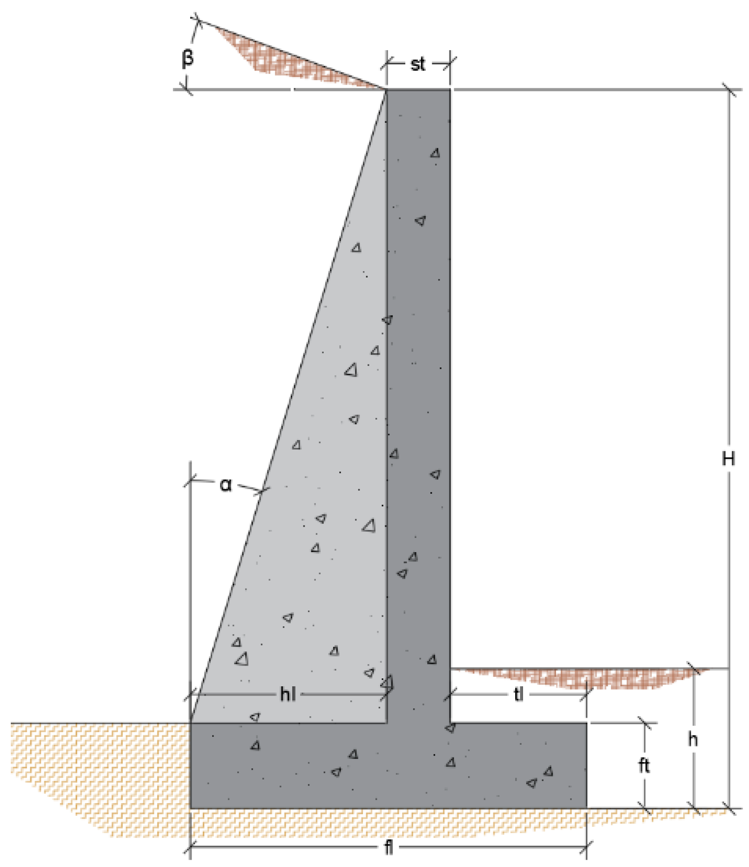
The design variables and parameters must be defined to describe the constructive solution, which are the variable and fixed data, respectively. Table 2 shows the 20 variables that define the buttressed wall design. Table 3 indicates the descriptions of the parameters and their values. Furthermore, Figure 1 and Figure 2 show the geometric variables represented in an outline and Figure 3 shows the reinforcement variables. The fill considered [43] corresponds to granular soils with more than 12% of fines (GM, GC, SM, SC, in accordance with the Unified Soil Classification System) and fine soils with more than 25% of coarse fraction soils (45 mm or less). The soil is characterized by 30° of an internal friction angle and a density (γ) of 20 kN/m3. The foundation soil maximum bearing capacity considered was 0.3 MPa [43].
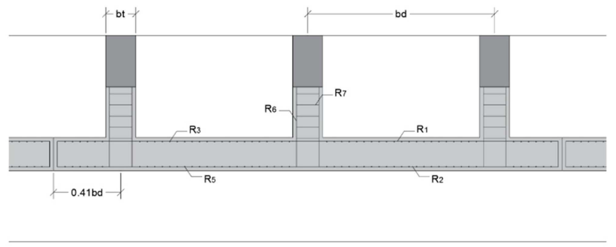
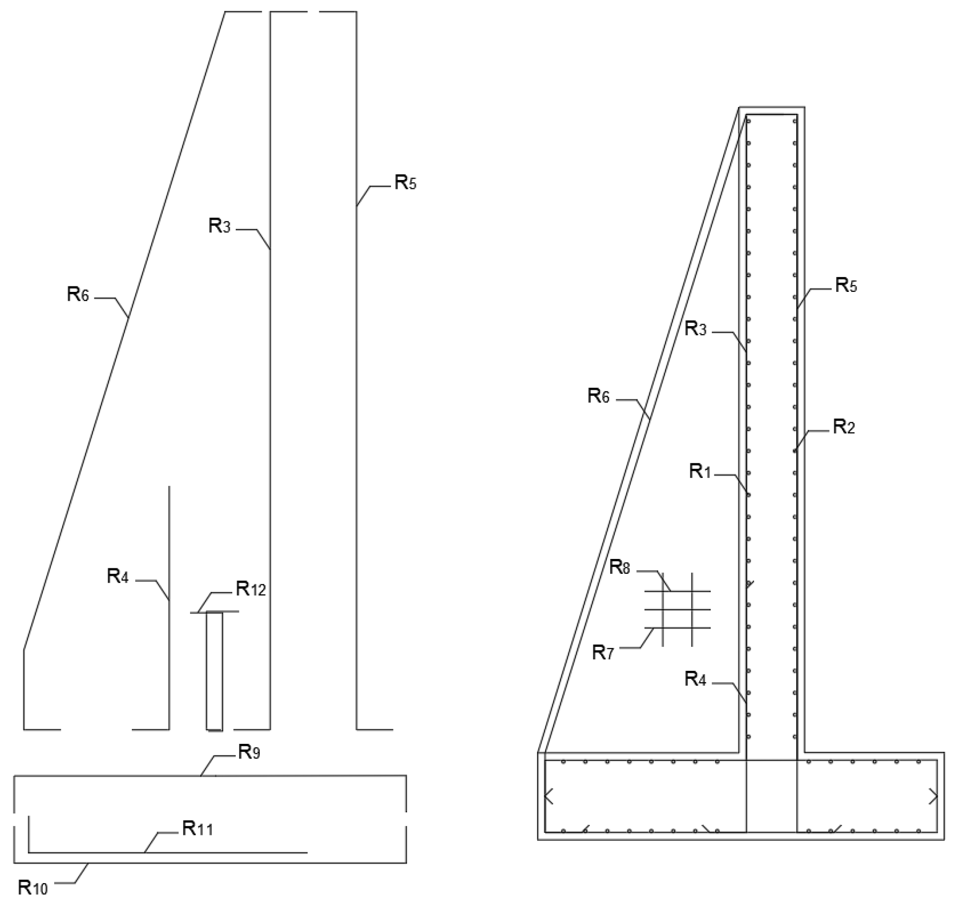
Usually, the amount of steel increases with the wall height and decreases with the increase in bearing capacity and cohesion of the ground. Taking all design variables and combining them, a solution space is created. These variables are linked to the geometry of the wall, the reinforcement amount, and the concrete and steel grades. Variables are the same as in the study of Molina-Moreno et al. [44]. On the one hand, the variables related to the geometry of the wall are (Figure 1 and Figure 2): footing thickness (ft), stem thickness (st), toe (tl) and heel (hl) lengths, buttress thickness (bt), distance between them (bd), angle of buttresses (α), fill slope (β), and foundation depth (h). On the other hand, the variables related to the reinforcement position and amount are R1 to R12 (Figure 3).
Variables R1 to R4 are related to the flexural bending of the stem, R1 to R3 resist the main bending moment, while R4 acts as a bending reinforcement at the bottom of the stem. The reinforcement related to the resistance of the thermal effects and shrinkage are the longitudinal bars represented by R5. The buttress needs a longitudinal reinforcement that materializes with the R6 reinforcement. R7 and R8 represent the reinforcement area of the bottom of the buttress. R9 and R11 are the bottom and upper footing reinforcement bars and R12 is the shear reinforcement one. R10 is the reinforcement that resists the longitudinal effects on the footing.
2.2. Structural Analysis
The placement of buttresses, usually at the back of the wall, means that the slab can be modelled as a continuous slab on supports. The placement of the buttresses on the inner part allows the rigidity of the joining system against flexural bending stresses to be the necessary one. In this way, the upper part works as a T-shaped section. The wall works as a section with a variable edge in a bracket where the edge is maximum in the area where the stem joins the foundation. The structure becomes hyperstatic because of the constraints suffered by both the stem and the foundation due to the existence of the buttresses. The buttress was calculated in the same way as a cantilevered T-beam and the sections were checked at different depths. Horizontal deflection is similar to a continuous slab supported on pillars because of the reduced dimensions of the cross-section of the stem of the buttresses. In the structural analysis, the buttress was considered to work as the web of a T-beam with a depth that varied in relation to the depth of the wall.
The structural checks carried out were those indicated in the Spanish regulations and recommendations [45,46]. The ultimate limit states of shear and bending and the serviceability limit state of cracking were verified. The hyperstatic structure testing method used was that by Huntington [47]. All limit states were calculated taking into account a uniform overload on the slope surface [41]. The wall earth pressures were calculated from the characteristics of the backfill and the surface loads. The forces used for the calculation of the stem were: horizontal ground thrust, elevation weight, heel weight, toe weight, surface load, and passive resistance exerted by the ground on the toe. The stresses on the buttresses were calculated according to the horizontal pressure of the ground in the stem and the spacing between buttresses.
The effects of bending moment and shear in the stem are reduced by the effect of the buttresses placed at a distance (db). The top of the stem works as a cantilever, while the lower part is coerced by the embedding in the foundation at the base of the buttresses. Equations (4) and (5) give the value of the bending moments that appear in the middle section between buttresses:
In Equations (4) and (5), p1 represents the pressure in the contact zone of the stem with the footing, M1 is the bending moment in this zone, and M2 is the maximum bending moment produced in the stem slab. Equation (6) shows the value of the shear resistance at the connection of the stem to the footing if the value of the distance between buttresses is less than half the height:
The distribution of pressures due to flexural stresses between the different stem spans can be considered trapezoidal [47]. The maximum value of these stresses is at the top of the foundation. The bending moment is one of the constraints that conditions the cross-sections and can therefore be used to define the thickness of those sections. Vertical bending moment is neglected in Huntington’s calculation method [47].
For the bending check of the T-cross-sections, the effective width was obtained, as indicated in the Model Code [48]. The expressions to evaluate the mechanical strength of the sections were obtained from Calavera [41]. In these expressions, the restrictions imposed by the Spanish Structural Concrete Code [46] were considered. In addition to the resistance checks of the sections, the overturning and sliding of the wall were also checked. On the one hand, to satisfy the overturning condition, the favorable moments must be greater than the unfavorable ones, considering an overturning safety factor of 1.8 for frequent events. On the other hand, the sliding verification consists of a comparison between the frictional force produced by the weight of the wall elements and the earth on the toe and heel added to the passive resistance generated by the terrain in the toe area compared with the horizontal reaction produced by the terrain at the back of the wall.
All checks were performed per linear meter of wall. The section strength checks carried out were bending and shear. In addition, the verification module itself checked the compliance of minimum reinforcement amount in accordance with the recommendations of Calavera [41] and, finally, checked that the reaction in the ground was less than two times greater than the bearing capacity.
2.3. Optimization Algorithm
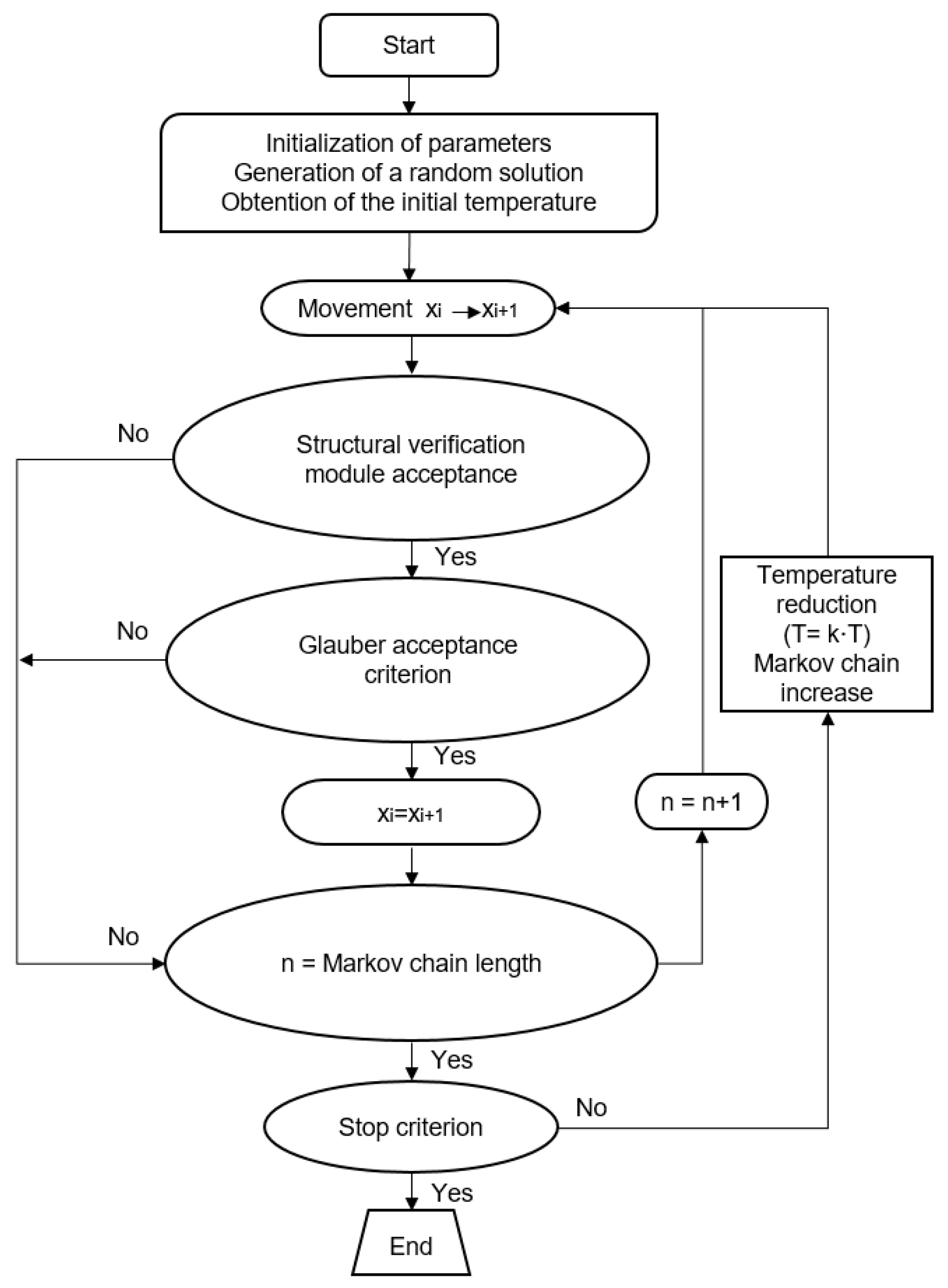
The optimization algorithm applied in this work was a hybrid simulated annealing (SA) algorithm. The algorithm was selected from the study by Yepes et al. [49] and modified using a mutation operator (SAMO2). This algorithm allows a combination of the advantages of the diversity of genetic algorithms with the good convergence of SA. The SA algorithm, proposed by Kirkpatrick et al. [50], simulates the formation of crystals to reach optimum solutions. The parameter that controls the probability of acceptance of higher cost or EE solutions is the temperature (T). This parameter starts with an initial value T0 and, as the algorithm generates solutions, the temperature decreases, allowing less acceptance of higher cost or EE solutions. The initial value of the temperature is determined by the procedure proposed by Medina [51]. The probability of acceptance, Pa, depends on the temperature and the increment between the new and old solution, ΔE. This function (Equation (7)) proposed by Glauber [52] can reject better solutions. On the other hand, the promotion of diversity is introduced in this algorithm by the generation of new solutions through a mutation operator. Holland [53] studied the search for good solutions by introducing the concepts of selection, crossover, and mutation in a mutation operator. Soke and Bingul [54] combined the two algorithms effectively. Figure 4 illustrates a flowchart of the SAMO2 process.
The parameters used in this study in relation to cost optimization were the following: length of Markov chains of 25,000, cooling coefficient of 0.90, simultaneous variable changes per movement of 5%, and number of unimproved Markov chains of 1. The algorithm stopped when the temperature was lower than 5% of the initial temperature. For energy optimization, the parameters used were length of Markov chains of 25,000, cooling coefficient of 0.95, simultaneous variable changes per movement of 3%, and number of unimproved Markov chains of 1. To obtain the value of these parameters, a tuning was carried out. The parameters were obtained by a tuning process to obtain those which gave good results for all calculated wall heights, reducing deviation of the results in terms of energy consumption up to 2.26% for a 12 m wall height.
The algorithm was programmed in MATLAB® and run using Intel® CoreTM i7-3820 CPU with 3.60 GHz. The computing time needed to run the algorithm and to obtain one solution was five minutes. In this study, we calculated nine walls for each height and objective function considered [43].
3. Results of the Parametric Study
In this parametric study, we have considered one linear meter of wall as a unitary reference value. Because of this, we have considered the variation of the main parameters in relation to the wall height for this unitary reference value. This study was performed for wall heights between 6 and 15 m with an increment of 1 m between them. The limits set for wall heights were set in accordance with those used in the article by Molina-Moreno et al. [44], reducing the values of heights to those whose results converged for the algorithm used for the optimization. The results between the energy and cost optimization were compared for different variables. Furthermore, we analyzed the influence of the concrete and reinforcing steel amounts for the two different objective functions. All the values gathered on the figures are the average values of the nine iterations carried out for each point.
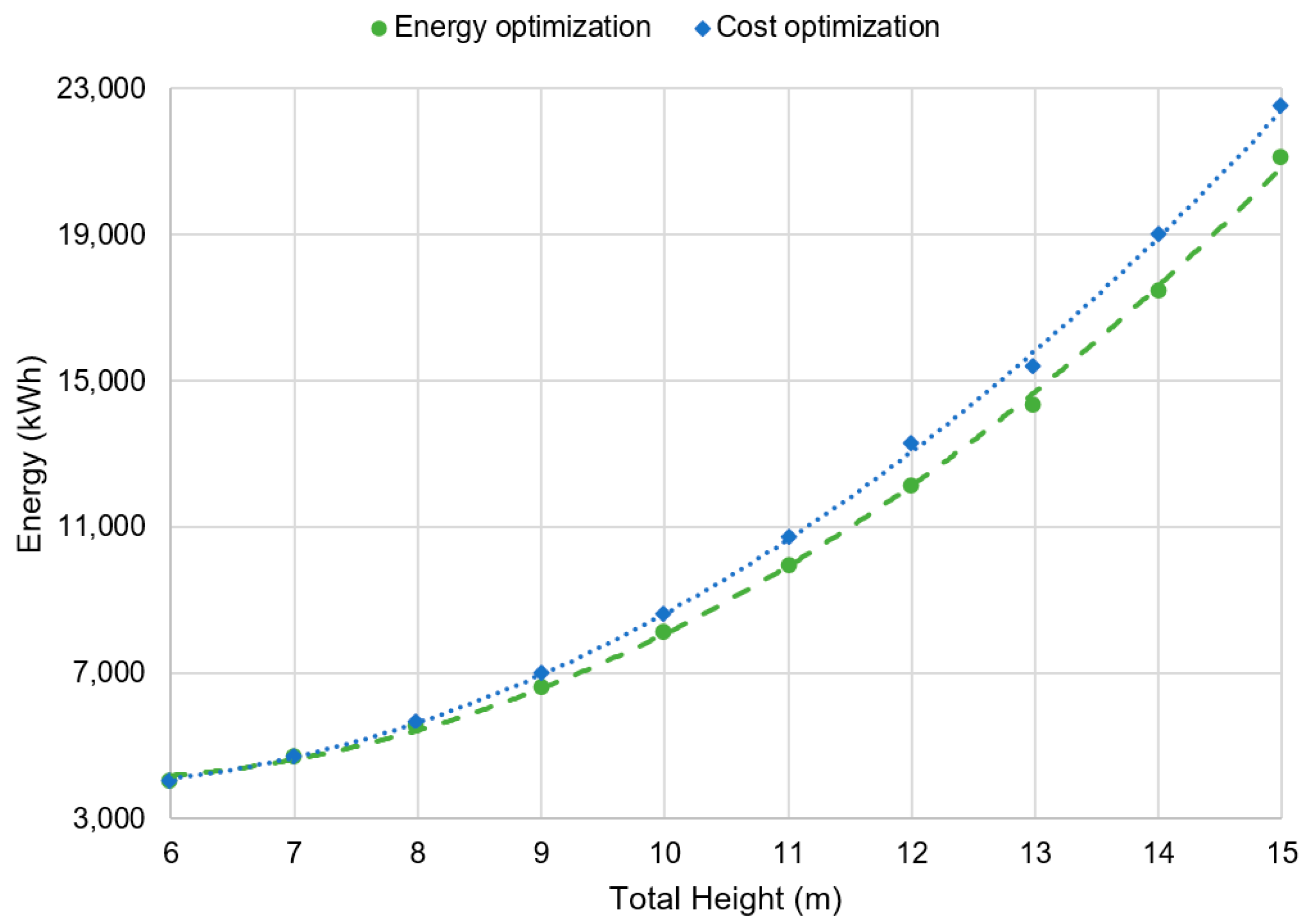
Figure 5 shows the trend of the values of cost, comparing energy and cost optimizations. As expected, energy optimization shows higher cost values compared with cost optimization. The embodied energy optimization objective function gives the values of cost adjusted to a parabolic curve, C = 36.644 H2 − 299 H + 1834.1, with a correlation coefficient of R² = 0.9998. In the same way, the embodied energy values obtained by embodied energy optimization adjust to E = 176.15 H2 − 1845.9 H + 8916.5, with a correlation coefficient of R² = 0.9992, as shown in Figure 6. The increase in the cost and the emissions related to the increase in the wall height are not linear and increase faster as the height grows.
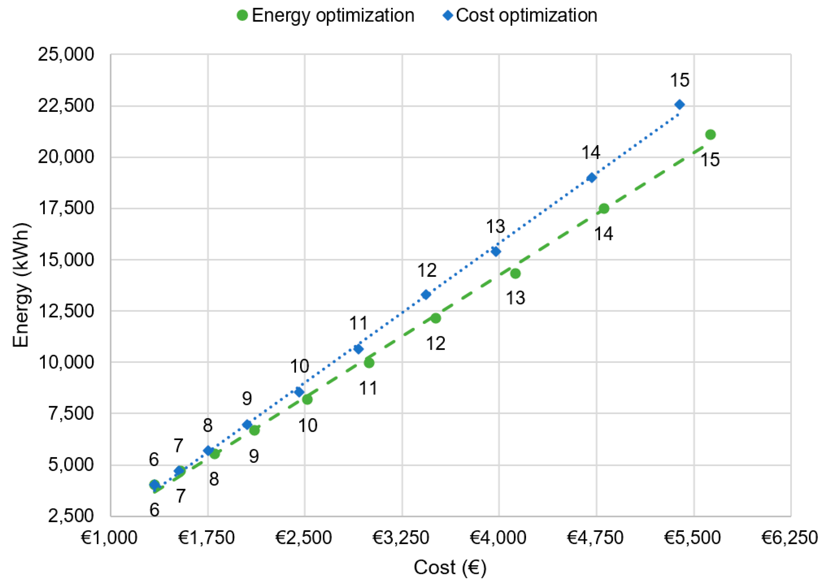
As we can see in Figure 7, the trend of cost and energy are both linear if we compare energy with cost obtained for each optimization, this conducts us to the conclusion that both optimization objectives are linked. If we look at the slope of the cost optimization line, its value corresponds to 4.54, this means that a cost reduction of €1 produces a saving of 4.54 kWh of EE.
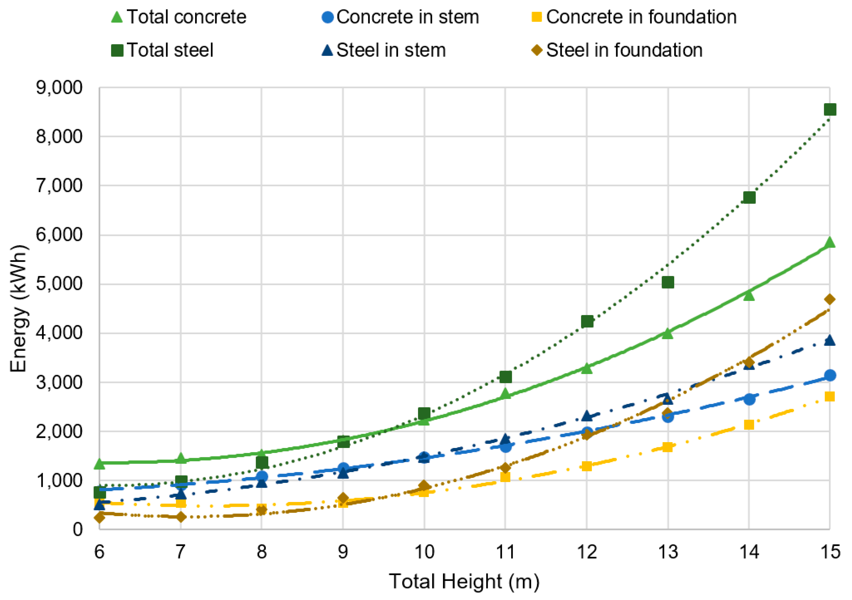
Figure 8 displays the embodied energy associated with the amount of steel and concrete obtained by the embodied optimization process. As shown, the energy wasted by concrete is lower than steel from 6 to 9.5 m; from this height, the energy consumed by the concrete exceeds steel. This is due to the fact that concrete is capable of resisting the stresses up to a certain height of the wall, and after that point, it is necessary to largely increase the amount of steel to support the stresses. This energy consumption change is produced at the same time in the stem and foundation. The amount of concrete is always greater in the stem than in the foundation; however, if we focus on steel consumption, a change around 13.5 m of wall height can be observed, where the steel in the stem starts to be greater than the steel in the foundation.
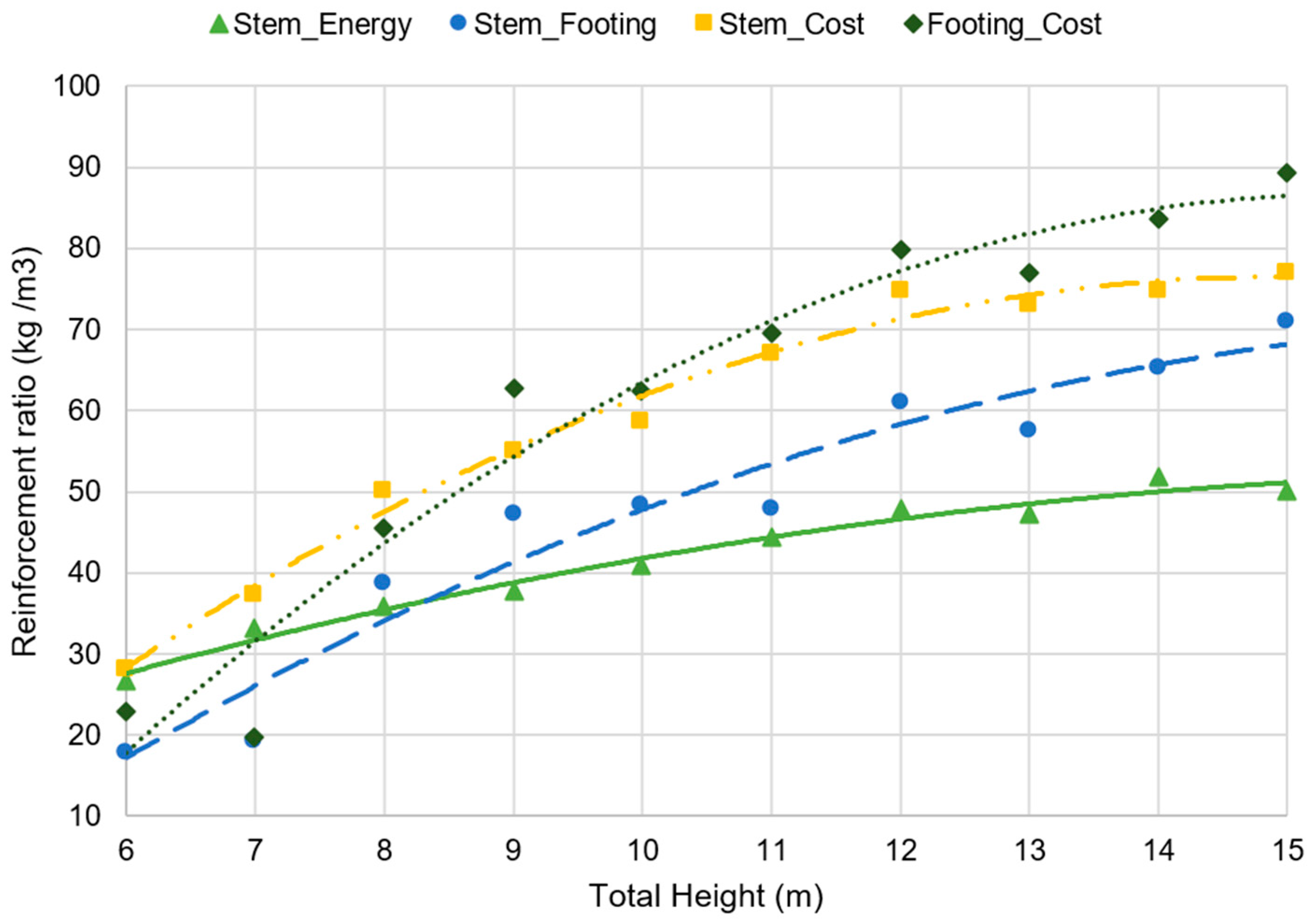
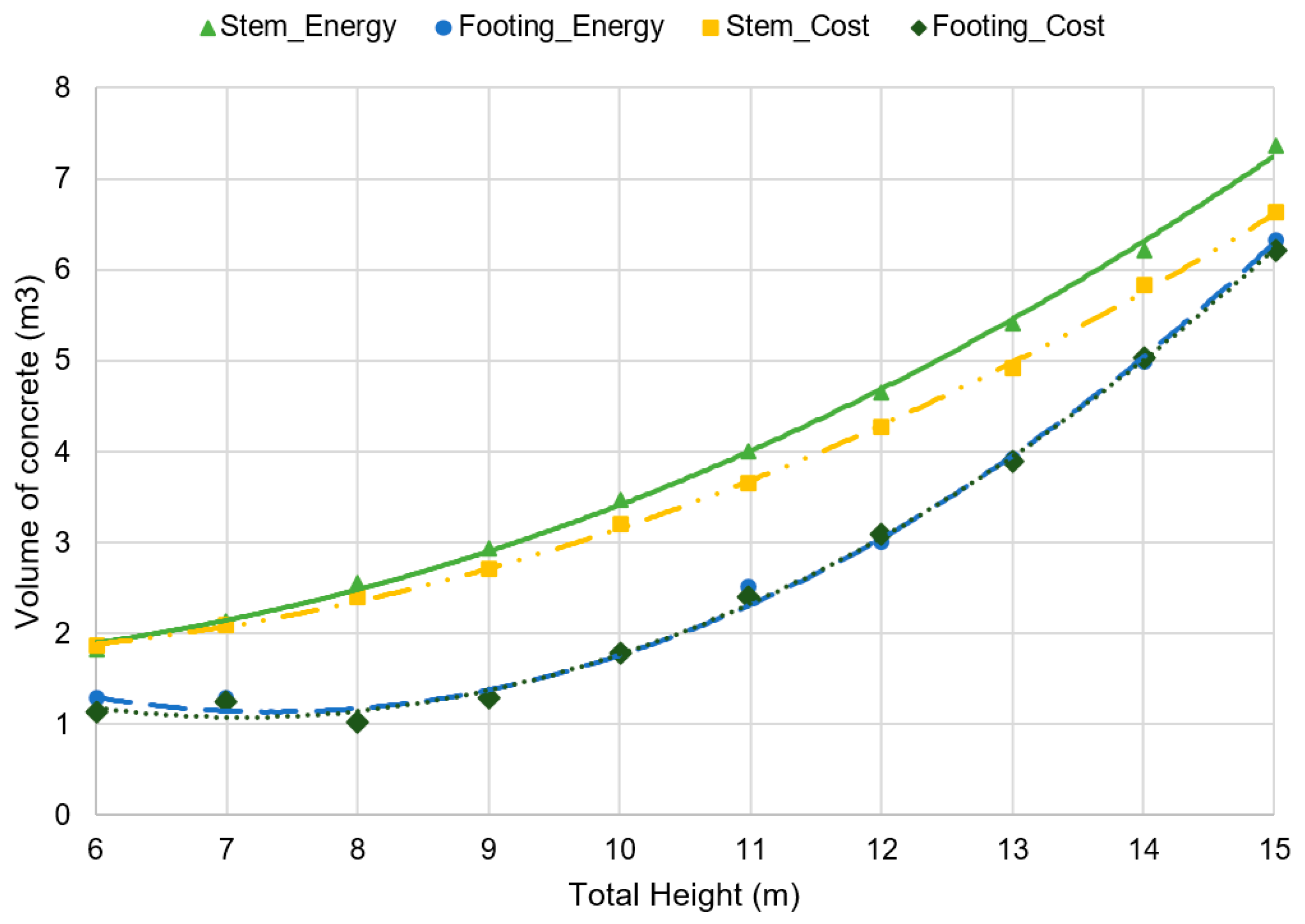
It is important to obtain pre-dimensioning rules to obtain the reinforcement by each cubic meter of concrete and the volume of concrete used to build one meter of wall. In Figure 9 and Figure 10, this data is shown for stem and footing due to the dependence of the results from the foundation on the characteristics of the terrain. As shown in Figure 9, the trend of the reinforcement ratio is parabolic to cost and embodied energy optimizations: the embodied energy optimization adjusts to Rs = −0.1853 H2 + 6.5067 H − 4.755, with a R² = 0.9781 for the stem, and Rf = −0.3959 H2 + 13.978 H − 52.406, with a R² = 0.9403 for the footing. The expression used to obtain the global reinforcement ratio for 1 m of wall is parabolic and adjusted to R = −0.2165 H2 + 8.502 H − 19.618, with a R² = 0.9818. All adjustments have a good correlation coefficient, assuring a good prediction of the amount of reinforcing steel per cubic meter of concrete. In addition, the volume of concrete is shown in Figure 10: the trend of adjustment is parabolic, as in the case for reinforcing steel, with the expression of concrete volume for the embodied energy optimization being Vcs = 0.0433 H2 − 0.3137 H + 2.2213, with a R² = 0.9984 for the stem, and Vcf = 0.0881 H2 − 1.294 H + 5.8902, with a R² = 0.9969 for the footing. The expression of the global volume of concrete adjusts to Vc = 0.1313 H2 − 1.6074 H + 8.11, with a R² = 0.9989. You can observe that the embodied energy optimization gives a higher value of concrete volume than the cost optimization in contrast with the reinforcing steel amount, where the embodied energy gives a lower amount. Both optimizations have resulted in a concrete compressive strength of 25 MPa (C25/30) and B500 steel grade for all cases studied. This is because the cost and energy consumed increase as the resistance of the concrete increases and, therefore, varying the geometry and modifying the quantities of materials gives better results than varying the characteristic resistance of the concrete.
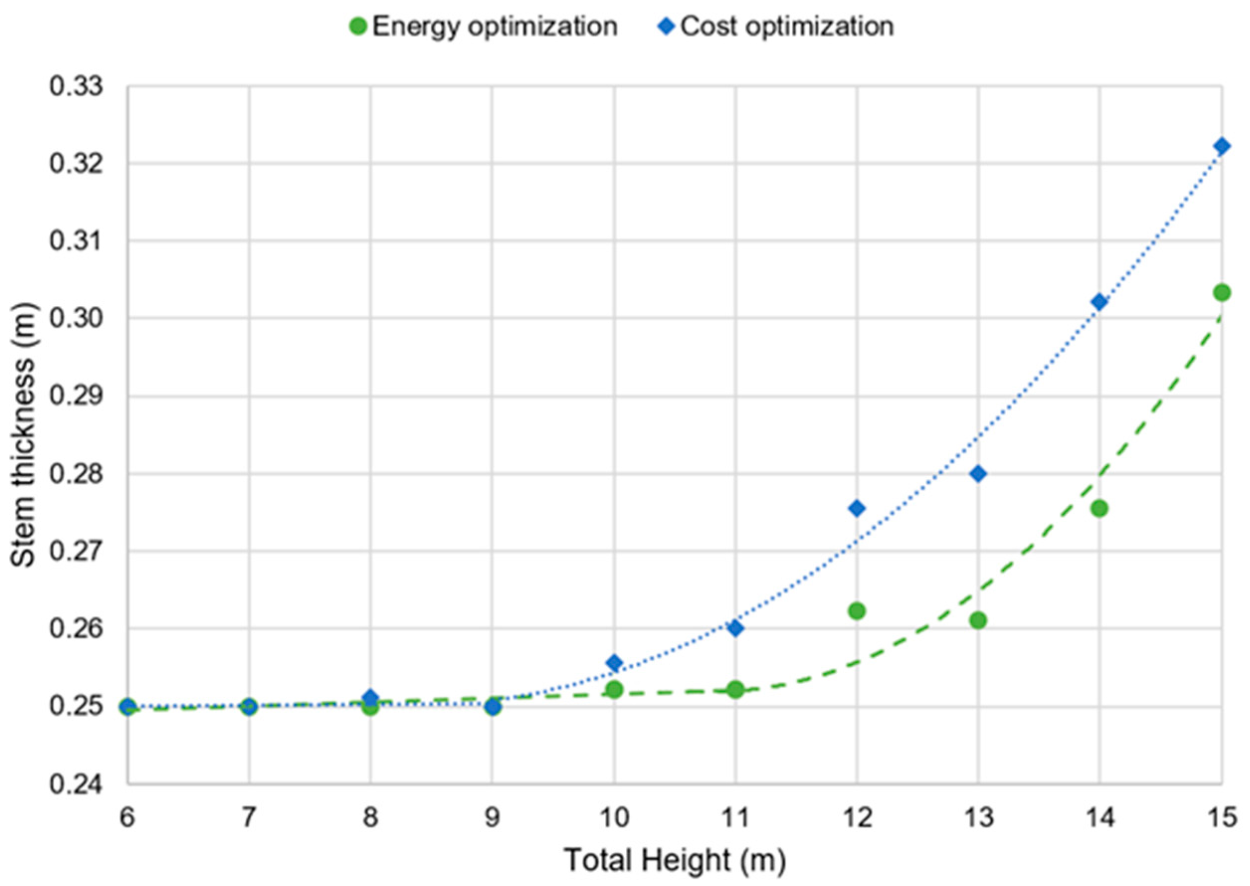
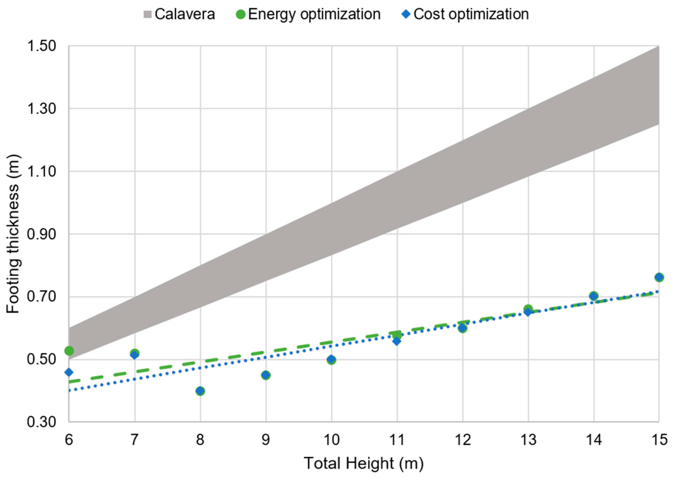
Once the cost, energy, and the amount of materials were obtained, the geometrical variables obtained by the optimization procedures were studied to analyze the variations between cost and energy results. The largest differences between the geometrical variables were produced in the stem thickness (st) and in the buttress distance (bd), while the difference between the foundation geometry obtained by the two optimization objectives is negligible, giving both optimization objectives the same values. Figure 11 shows the values obtained at the stem thickness (st). It can be observed that, from 6 to 11 m, the stem thickness obtained is 0.25 m for the two optimizations, but from 11 m of wall height upwards, the embodied energy optimization takes on a parabolic trend equal to st = 0.0028 H2 − 0.0607 H + 0.5809, with a R² = 0.9533. The cost optimization shows higher values of stem thickness from 9 m upwards compared with the embodied energy expression. The values obtained from the optimization take the lower limit imposed by the constructive facility of these types of structures; from this point, a greater thickness of wall is needed to resist the efforts. Figure 12 displays the results for the buttress distance, showing that the embodied energy optimization takes lower values for the buttress distances. A shorter distance allows a reduction in the flexural moments and, as a consequence, the need for reinforcing steel at the expense of increasing the concrete amount. This result shows how embodied energy optimization allows us to reduce the amount of reinforcing steel to reach a lower amount of total embodied energy. The expression of the linear trend obtained is bd = 0.0567 H + 2.4546, with a R² = 0.4435. Furthermore, the results obtained by this optimization have been compared with the Calavera recommendations [41] in Figure 13; as can be seen, the cost optimization is inside the area defined by the geometrical limits defined as the buttresses distance by Calavera (H/3 to H/2), while the energy optimization is only inside from 6 to 10 m.
From a 10 m wall height, energy optimization takes lower values from the distance between buttresses. In addition, the comparison between the footing thickness obtained by this optimization procedure and the values provided by Calavera [41] were compared. Both the optimization with an energy objective and a cost objective give values of H/20, while the limits imposed by Calavera are between H/12 and H/10, as shown in Figure 13. These footing thickness results are similar to those obtained by Molina-Moreno et al. [44], who also obtained values lower than those in the recommendations by Calavera.
Finally, the footing geometrical variables are displayed. The difference between the cost and embodied energy optimization is almost indiscernible. The toe length (tl) remains constant at 7 m and then it has a linear trend equal to tl = 0.2114 H − 1.3387, with a good correlation coefficient of R² = 0.9935. Something similar occurs to the heel length (hl), which remains constant at 9 m of wall height and from this point onwards, adjusts to a linear expression equal to hl = 0.67 H − 4.2098, with a R² = 0.9798. The results of the analysis show that the main difference between the cost and the embodied energy optimizations is produced in the geometry of the stem and buttresses, which generate a difference in the amount and distribution of materials.
4. Conclusions
In this paper, cost and embodied energy optimizations were applied to a buttressed wall. The results of the two optimizations were compared to determine the differences between cost and energy optimum designs. The optimization algorithm used in this study was a hybrid simulated annealing with a mutation operator.
The EE optimization shows, as expected, a lower EE amount at the expense of a small increase in cost. In light of this, it can be said that there is a clear relation between the two-optimization objectives. If EE is considered as an objective function, a slightly higher cost will be obtained for each of the wall heights, but it will always be linked to a cost reduction due to the connection between the two optimization objectives. A cost reduction of €1 produces a saving of 4.54 kWh of EE. Focusing the study on material amounts, it was observed that EE optimization gives lower amounts of reinforcing steel and greater amounts of concrete from 6 to 9.5 m. This variation of material amounts compared with cost optimization is produced because of the reduction of the stem thickness and the buttress distance, which allows a reduction in the flexural moments in the stem for EE optimization. If the comparison is focused on buttress distance, it can be noted that the values obtained by the cost optimization are inside the area defined by the geometrical limits imposed on the buttress distance by Calavera (H/3 to H/2). The energy optimization is only inside the limits from 6 to 10 m and, from 10 m on, lower values are obtained. The geometrical variables of the footing are roughly equal for both cost and energy optimum design, with differences so slight that they can be disregarded. If the design obtained by the optimization procedure is compared with the recommendations published by Calavera, it can be observed that the values of footing thickness are lower than those imposed by the author. The values obtained for the footing thickness are H/20, while the design limits proposed by Calavera are H/12 and H/10.
This paper not only showed a comparison between two optimization criteria, but also provided rules of pre-dimensioning for engineers and other technicians working in civil engineering. The study allows engineering to attain embodied energy optimum designs by applying the expressions obtained from the results of the optimization. This paper helps to establish a good design for an earth-retaining buttressed wall and opens the door to other researchers who will develop automated designs to reduce the impact of these structures.
Author Contributions
This paper represents a result of teamwork. The authors jointly designed the research. D.M.-M. drafted the manuscript, and J.V.M., J.G. and V.Y. edited and improved the manuscript until all authors were satisfied with the final version. All authors have read and agreed to the published version of the manuscript.
Funding
The authors acknowledge the financial support of the Spanish Ministry of Economy and Business, along with FEDER funding (DIMALIFE Project: BIA2017-85098-R) and the Spanish Ministry of Science, Innovation and Universities for David Martínez-Muñoz University Teacher Training Grant (FPU18/01592). They would also like to emphasize that José García was supported by the Grant CONICYT/FONDECYT/INICIACION/11180056.
Institutional Review Board Statement
Not applicable.
Informed Consent Statement
Not applicable.
Data Availability Statement
The results of the experiments are in: https://drive.google.com/file/d/15ZL5f-UHNo2wWEGSn7l6ixUgV77G9Whj/view?usp=sharing (accessed on 18 February 2021).
Conflicts of Interest
The authors declare no conflict of interest.
References
- World Commission on Environment and Development. Our Common Future. (The Brundtland Report); Oxford University Press: Oxford, UK, 1987. [Google Scholar]
- International Energy Agency. Key World Energy Statistics 2019; IEA: Paris, France, 2019. [Google Scholar]
- Casals, X.G. Analysis of building energy regulation and certification in Europe: Their role, limitations and differences. Energy Build. 2006, 38, 381–392. [Google Scholar] [CrossRef]
- Sartori, I.; Hestnes, A.G. Energy use in the life cycle of conventional and low-energy buildings: A review article. Energy Build. 2007, 39, 249–257. [Google Scholar] [CrossRef]
- Reap, J.; Roman, F.; Duncan, S.; Bras, B. A survey of unresolved problems in life cycle assessment. Part 1: Goal and scope and inventory analysis. Int. J. Life Cycle Assess. 2008, 13, 290–300. [Google Scholar] [CrossRef]
- Reap, J.; Roman, F.; Duncan, S.; Bras, B. A survey of unresolved problems in life cycle assessment. Part 2: Impact assessment and interpretation. Int. J. Life Cycle Assess. 2008, 13, 374–388. [Google Scholar] [CrossRef]
- Dixit, M.K.; Fernández-Solís, J.L.; Lavy, S.; Culp, C.H. Identification of parameters for embodied energy measurement: A literature review. Energy Build. 2010, 42, 1238–1247. [Google Scholar] [CrossRef]
- Hernandez, P.; Kenny, P. From net energy to zero energy buildings: Defining life cycle zero energy buildings (LC-ZEB). Energy Build. 2010, 42, 815–821. [Google Scholar] [CrossRef]
- Chang, Y.; Ries, R.J.; Lei, S. The embodied energy and emissions of a high-rise education building: A quantification using process-based hybrid life cycle inventory model. Energy Build. 2012, 55, 790–798. [Google Scholar] [CrossRef]
- Farzampour, A.; Khatibinia, M.; Mansouri, I. Shape optimization of butterfly-shaped shear links using Grey Wolf algorithm. Ing. Sismica 2019, 36, 27–41. [Google Scholar]
- Ramesh, T.; Prakash, R.; Shukla, K. Life cycle energy analysis of buildings: An overview. Energy Build. 2010, 42, 1592–1600. [Google Scholar] [CrossRef]
- Fay, R.; Treloar, G.; Iyer-Raniga, U. Life-cycle energy analysis of buildings: A case study. Build. Res. Inf. 2000, 28, 31–41. [Google Scholar] [CrossRef] [Green Version]
- ISO. ISO 14040:2006—Environmental Management—Life Cycle Assessment—Principles and Framework; ISO: Geneva, Switzerland, 2006. [Google Scholar]
- WBCSD. Energy Efficiency in Buildings: Business Realities and Opportunities; WBCSD: Geneva, Switzerland, 2008. [Google Scholar]
- Zastrow, P.; Molina-Moreno, F.; García-Segura, T.; Martí, J.V.; Yepes, V. Life cycle assessment of cost-optimized buttress earth-retaining walls: A parametric study. J. Clean. Prod. 2017, 140, 1037–1048. [Google Scholar] [CrossRef]
- Orr, J.; Bras, A.; Ibell, T. Effectiveness of design codes for life cycle energy optimisation. Energy Build. 2017, 140, 61–67. [Google Scholar] [CrossRef]
- Shadram, F.; Mukkavaara, J. Exploring the effects of several energy efficiency measures on the embodied/operational energy trade-off: A case study of swedish residential buildings. Energy Build. 2019, 183, 283–296. [Google Scholar] [CrossRef]
- Yang, H.; Koopialipoor, M.; Armaghani, D.J.; Gordan, B.; Khorami, M.; Tahir, M.M. Intelligent design of retaining wall structures under dynamic conditions. Steel Compos. Struct. 2019, 31, 629–640. [Google Scholar]
- Azarafza, M.; Feizi-Derakhshi, M.R.; Azarafza, M. Computer modeling of crack propagation in concrete retaining walls: A case study. Comput. Concr. 2017, 19, 509–514. [Google Scholar] [CrossRef]
- Lee, C.I.; Kim, E.K.; Park, J.S.; Lee, Y.J. Preliminary numerical analysis of controllable prestressed wale system for deep excavation. Geomech. Eng. 2018, 15, 1061–1070. [Google Scholar]
- Song, F.; Tian, Y. Three-dimensional numerical modelling of geocell reinforced soils and its practical application. Geomech. Eng. 2019, 17, 1–9. [Google Scholar]
- Mergos, P.E. Seismic design of reinforced concrete frames for minimum embodied CO2 emissions. Energy Build. 2018, 162, 177–186. [Google Scholar] [CrossRef] [Green Version]
- Park, H.S.; Hwang, J.W.; Oh, B.K. Integrated analysis model for assessing CO2 emissions, seismic performance, and costs of buildings through performance-based optimal seismic design with sustainability. Energy Build. 2018, 158, 761–775. [Google Scholar] [CrossRef]
- Yepes, V.; Dasí-Gil, M.; Martínez-Muñoz, D.; López-Desfilis, V.J.; Martí, J.V. Heuristic Techniques for the Design of Steel-Concrete Composite Pedestrian Bridges. Appl. Sci. 2019, 9, 3253. [Google Scholar] [CrossRef] [Green Version]
- Yoon, Y.-C.; Kim, K.-H.; Lee, S.-H.; Yeo, D. Sustainable design for reinforced concrete columns through embodied energy and CO2 emission optimization. Energy Build. 2018, 174, 44–53. [Google Scholar] [CrossRef]
- Zhang, Z.; Pan, J.; Fu, J.; Singh, H.K.; Pi, Y.L.; Wu, J.; Rao, R. Optimization of long span portal frames using spatially distributed surrogates. Steel Compos. Struct. 2017, 24, 227–237. [Google Scholar]
- Minoglou, M.K.; Hatzigeorgiou, G.D.; Papagiannopoulos, G.A. Heuristic optimization of cylindrical thin-walled steel tanks under seismic loads. Thin Walled Struct. 2013, 64, 50–59. [Google Scholar] [CrossRef]
- Pan, Q.; Yi, Z.; Yan, D.; Xu, H. Pseudo-Static Analysis on the Shifting-Girder Process of the Novel Rail-Cable-Shifting-Girder Technique for the Long Span Suspension Bridge. Appl. Sci. 2019, 9, 5158. [Google Scholar] [CrossRef] [Green Version]
- Balasbaneh, A.T.; Marsono, A.K. Bin Applying multi-criteria decision-making on alternatives for earth-retaining walls: LCA, LCC, and S-LCA. Int. J. Life Cycle Assess. 2020, 25, 2140–2153. [Google Scholar] [CrossRef]
- Yeo, D.; Gabbai, R.D. Sustainable design of reinforced concrete structures through embodied energy optimization. Energy Build. 2011, 43, 2028–2033. [Google Scholar] [CrossRef]
- Yu, R.; Zhang, D.; Yan, H. Embodied Energy and Cost Optimization of RC Beam under Blast Load. Math. Probl. Eng. 2017, 2017, 1–8. [Google Scholar] [CrossRef]
- Penadés-Plà, V.; García-Segura, T.; Yepes, V. Accelerated optimization method for low-embodied energy concrete box-girder bridge design. Eng. Struct. 2019, 179, 556–565. [Google Scholar] [CrossRef]
- Foraboschi, P.; Mercanzin, M.; Trabucco, D. Sustainable structural design of tall buildings based on embodied energy. Energy Build. 2014, 68, 254–269. [Google Scholar] [CrossRef]
- Camp, C.V.; Akin, A. Design of Retaining Walls Using Big Bang–Big Crunch Optimization. J. Struct. Eng. 2012, 138, 438–448. [Google Scholar] [CrossRef]
- Kaveh, A.; Khayatazad, M. Optimal design of cantilever retaining walls using ray optimization method. Iran. J. Sci. Technol. Trans. Civ. Eng. 2014, 38, 261–274. [Google Scholar]
- Kayabekir, A.E.; Arama, Z.A.; Bekdaş, G.; Nigdeli, S.M.; Geem, Z.W. Eco-Friendly Design of Reinforced Concrete Retaining Walls: Multi-objective Optimization with Harmony Search Applications. Sustainability 2020, 12, 6087. [Google Scholar] [CrossRef]
- García, J.; Yepes, V.; Martí, J.V. A Hybrid k-Means Cuckoo Search Algorithm Applied to the Counterfort Retaining Walls Problem. Mathematics 2020, 8, 555. [Google Scholar] [CrossRef]
- Kalemci, E.N.; Ikizler, S.B. Rao-3 algorithm for the weight optimization of reinforced concrete cantilever retaining wall. Geomech. Eng. 2020, 20, 527–536. [Google Scholar]
- Yepes, V.; Martí, J.V.; García, J. Black Hole Algorithm for Sustainable Design of Counterfort Retaining Walls. Sustainability 2020, 12, 2767. [Google Scholar] [CrossRef] [Green Version]
- García, J.; Martí, J.V.; Yepes, V. The buttressed walls problem: An application of a hybrid clustering particle swarm optimization algorithm. Mathematics 2020, 8, 862. [Google Scholar] [CrossRef]
- Calavera, R.J. Muros de Contención Y Muros de Sótano, 3rd ed.; Intemac: Madrid, Spain, 2001; ISBN 8488764103. (In Spanish) [Google Scholar]
- Catalonia Institute of Construction Technology BEDEC ITEC Materials Database. Available online: https://metabase.itec.cat/vide/es/bedec (accessed on 1 January 2021).
- Yepes, V.; González-Vidosa, F.; Alcalá, J.; Villalba, P. CO2-Optimization Design of Reinforced Concrete Retaining Walls Based on a VNS-Threshold Acceptance Strategy. J. Comput. Civ. Eng. 2012, 26, 378–386. [Google Scholar] [CrossRef] [Green Version]
- Molina-Moreno, F.; García-Segura, T.; Martí, J.V.; Yepes, V. Optimization of buttressed earth-retaining walls using hybrid harmony search algorithms. Eng. Struct. 2017, 134, 205–216. [Google Scholar] [CrossRef]
- Ministerio de Fomento. CTE-DB-SE-C Seguridad Estructural Cimientos; Oficina de Vivienda Comunidad de Madrid: Madrid, Spain, 2007. [Google Scholar]
- Ministerio de Fomento. Instrucción de Hormigón Estructural (EHE-08); Gobierno de Espana: Madrid, Spain, 2008. [Google Scholar]
- Huntington, W.C. Earth Pressures and Retaining Walls; Wiley: Hoboken, NJ, USA, 1957. [Google Scholar]
- CEB. CEB-FIP MODEL CODE 1990; Thomas Telford Publishing: London, England, 1993. [Google Scholar]
- Yepes, V.; Alcala, J.; Perea, C.; González-Vidosa, F. A parametric study of optimum earth-retaining walls by simulated annealing. Eng. Struct. 2008, 30, 821–830. [Google Scholar] [CrossRef]
- Kirkpatrick, S.; Gelatt, C.D.; Vecchi, M.P. Optimization by Simulated Annealing. Science 1983, 220, 671–680. [Google Scholar] [CrossRef] [PubMed]
- Medina, J.R. Estimation of Incident and Reflected Waves Using Simulated Annealing. J. Waterw. Port Coastal Ocean Eng. 2001, 127, 213–221. [Google Scholar] [CrossRef]
- Glauber, R.J. Time-dependent statistics of the Ising model. J. Math. Phys. 1963, 4, 294. [Google Scholar] [CrossRef]
- Holland, J.H. Adaptation in Natural and Artificial Systems; The MIT Press: Cambridge, MA, USA, 1992. [Google Scholar]
- Soke, A.; Bingul, Z. Hybrid genetic algorithm and simulated annealing for two-dimensional non-guillotine rectangular packing problems. Eng. Appl. Artif. Intell. 2006, 19, 557–567. [Google Scholar] [CrossRef]
Figure 1.
Geometrical variables of the buttressed wall.

Figure 2.
Geometrical variables and reinforcements of the buttressed wall, cross-section.

Figure 3.
Reinforcement variables of the buttressed wall.

Figure 4.
Optimization process flowchart.

Figure 5.
Relation between cost and wall height.

Figure 6.
Relation between embodied energy and wall height.

Figure 7.
Relation between embodied energy and cost for the wall heights of the study, in m.

Figure 8.
Relation between embodied energy and cost.

Figure 9.
Relation between reinforcement ratio and wall height.

Figure 10.
Relation between volume of concrete and wall height.

Figure 11.
Relation between stem thickness and wall height.

Figure 12.
Relation between buttress distance and wall height.

Figure 13.
Relation between footing thickness and wall height.


Table 1.
Prices and embodied energy values of the construction units [42].
Table 1.
Prices and embodied energy values of the construction units [42].
| Unit | Energy (kW·h) | Cost (€) |
|---|---|---|
| Earth movement | ||
| m3 of backfill | 78.32 | 14.12 |
| m3 of backfill over the toe | 76.52 | 12.52 |
| m3 of earth excavation | 44.65 | 10.56 |
| Foundation | ||
| kg of steel B400 | 10.39 | 1.11 |
| kg of steel B500 | 10.39 | 1.13 |
| m3 of concrete C25/30 | 413.28 | 90.74 |
| m3 of concrete C30/37 | 439.51 | 99.44 |
| m3 of concrete C35/45 | 457.05 | 119.48 |
| m3 of concrete C40/50 | 477.98 | 122.5 |
| m3 of concrete C45/55 | 484.49 | 125.45 |
| m3 of concrete C50/60 | 492 | 127.93 |
| m2 of cleaning concrete | 24.8 | 9.28 |
| m2 of formwork | 6.56 | 23.83 |
| Stem | ||
| kg of steel B400 | 10.4 | 1.29 |
| kg of steel B500 | 10.4 | 1.31 |
| m3 of concrete C25/30 | 427.78 | 101.99 |
| m3 of concrete C30/37 | 454.01 | 110.69 |
| m3 of concrete C35/45 | 480.32 | 130.73 |
| m3 of concrete C40/50 | 511.72 | 133.84 |
| m3 of concrete C45/55 | 524.48 | 136.91 |
| m3 of concrete C50/60 | 535.74 | 140.98 |
| m2 of formwork | 86.57 | 53.26 |
Table 2.
Discrete design variables description.
| Variable | Unit | Description | Step Size | Lower Bound | Upper Bound |
|---|---|---|---|---|---|
| ft | cm | Footing thickness | 1 | H/14 | H/6 |
| st | cm | Stem thickness | 1 | 25 | 224 |
| tl | cm | Toe length | 1 | 20 | 819 |
| hl | cm | Heel length | 1 | 20 | 2019 |
| bt | cm | Buttress thickness | 2.5 | 25 | 172.5 |
| bd | cm | Distance between buttresses | 5 | 320 | 800 |
| fck | MPa | Concrete compressive strength | 5 | 25 | 50 |
| fyk | MPa | Steel yield strength | 100 | 400 | 500 |
| R1 to R10 (n) | Reinforcement number of bars | 1 | 2 | 17 | |
| R11 to R12 (n) | Reinforcement number of bars | 1 | 4 | 10 | |
| R1 to R12 (Ø) | mm | Reinforcement diameter | 6, 8, 10, 12, 16, 20, 25, 32 | ||
Table 3.
Parameters of the buttressed wall.
| Parameter | Value | |
|---|---|---|
| Maximum bearing capacity | σadm | 0.3 MPa |
| Fill slope | β | 0° |
| Foundation depth | h | 2 m |
| Uniform load on top of the fill | q | 10 kN/m2 |
| Wall-fill friction angle | δ | 0° |
| Base friction coefficient | μ | tg 30° |
| Safety coefficient against sliding | γfs | 1.5 |
| Safety coefficient against overturning | γto | 1.8 |
| Load safety coefficient | γG | 1.35 |
| Concrete safety coefficient | γc | 1.5 |
| Steel safety coefficient | γs | 1.15 |
| External ambient exposure | IIa | |
Publisher’s Note: MDPI stays neutral with regard to jurisdictional claims in published maps and institutional affiliations. |
© 2021 by the authors. Licensee MDPI, Basel, Switzerland. This article is an open access article distributed under the terms and conditions of the Creative Commons Attribution (CC BY) license (http://creativecommons.org/licenses/by/4.0/).
Share and Cite
MDPI and ACS Style
Martínez-Muñoz, D.; Martí, J.V.; García, J.; Yepes, V. Embodied Energy Optimization of Buttressed Earth-Retaining Walls with Hybrid Simulated Annealing. Appl. Sci. 2021, 11, 1800. https://0-doi-org.brum.beds.ac.uk/10.3390/app11041800
AMA Style
Martínez-Muñoz D, Martí JV, García J, Yepes V. Embodied Energy Optimization of Buttressed Earth-Retaining Walls with Hybrid Simulated Annealing. Applied Sciences. 2021; 11(4):1800. https://0-doi-org.brum.beds.ac.uk/10.3390/app11041800
Chicago/Turabian StyleMartínez-Muñoz, David, José V. Martí, José García, and Víctor Yepes. 2021. "Embodied Energy Optimization of Buttressed Earth-Retaining Walls with Hybrid Simulated Annealing" Applied Sciences 11, no. 4: 1800. https://0-doi-org.brum.beds.ac.uk/10.3390/app11041800
Note that from the first issue of 2016, this journal uses article numbers instead of page numbers. See further details here.