
Control of DC Motors to Guide Unmanned Underwater Vehicles


Sibley School of Mechanical and Aerospace Engineering, Cornell University, Ithaca, NY 14853, USA
Appl. Sci. 2021, 11(5), 2144; https://0-doi-org.brum.beds.ac.uk/10.3390/app11052144
Submission received: 20 January 2021
/
Revised: 20 February 2021
/
Accepted: 24 February 2021
/
Published: 28 February 2021
(This article belongs to the Special Issue Underwater Vehicles)
Abstract
:Many research manuscripts propose new methodologies, while others compare several state-of-the-art methods to ascertain the best method for a given application. This manuscript does both by introducing deterministic artificial intelligence (D.A.I.) to control direct current motors used by unmanned underwater vehicles (amongst other applications), and directly comparing the performance of three state-of-the-art nonlinear adaptive control techniques. D.A.I. involves the assertion of self-awareness statements and uses optimal (in a 2-norm sense) learning to compensate for the deleterious effects of error sources. This research reveals that deterministic artificial intelligence yields 4.8% lower mean and 211% lower standard deviation of tracking errors as compared to the best modeling method investigated (indirect self-tuner without process zero cancellation and minimum phase plant). The improved performance cannot be attributed to superior estimation. Coefficient estimation was merely on par with the best alternative methods; some coefficients were estimated more accurately, others less. Instead, the superior performance seems to be attributable to the modeling method. One noteworthy feature is that D.A.I. very closely followed a challenging square wave without overshoot—successfully settling at each switch of the square wave—while all of the other state-of-the-art methods were unable to do so.
1. Introduction
Carl Friedrich Gauss is often credited with the development of the least squares method [1], which can be done recursively, as well-described by Bierman [2]. Various instantiations of recursive least squares estimation algorithms have often been combined with modeling assumptions to produce adaptive decision and control methods; for example, the self-tuning regulators introduced by Kalman [3]. Not long afterward, two similar algorithms based on least squares and minimum variance control emerged. The first was presented by Peterka in Prague at an International Federation on Automatic Control conference [4], followed shortly after by Wieslander and Wittenmark’s publication of an adaptive control using real time identification [5]. This lineage established the paradigm that exists today: adaption in two parts—modeling and estimation. From this auspicious inception, self-tuning regulators remain foundational, being first analyzed thoroughly and presented by Åström and Wittenmark [6], and later revised [7], at which point the term self-tuning regulator was adopted. Åström and Wittenmark later produced a seminal text [8] elaborating on self-tuning regulators, with several variations on modeling assumptions and estimation algorithms in addition to model-reference adaptive control topologies. This text included sections on persistent excitation and parameter convergence—as did Slotine and Li’s text [9], which also included analytic methods for proving stability of the resulting time-varying nonlinear systems.
More recently, published comparative analyses fixed all factors except the modeling approach and/or the chosen estimation method, to produce advice regarding which methods to use to control direct current (DC) motors. While [10] illustrated quick methods to decide model degree based on minimizing estimation error, [11] compared indirect and direct self-tuning models with various degrees of pole excess, with and without plant cancelling.
Subsequently, several authors have published research incorporating learning methods into self-tuning control algorithms. Rubaai and Kotaru [12] tackled the problem of speed control of a DC motor using feedforward artificial neural networks to capture and emulate detailed nonlinear mappings and implement a full nonlinear control law.
Liu et al. [13] addressed the problem of DC motor speed control using a constant gain feedback controller (which failed to counter dynamic load torques)—using artificial neural networks to identify and control online, and therefore modulate control rate. Mishra [14] used artificial neural networks (ANNs) in estimating and controlling speed for a separately excited DC motor, (one in which the rotor speed can be made to follow an arbitrarily selected trajectory to achieve accurate trajectory control of the speed, especially when the motor and load parameters are unknown). Hernández-Alvarado et al. [15] proposed neural network-based self-tuning proportional, integral, and derivative (PID) control for underwater vehicles. Due to difficulties designing based on cost functions, the controllers were trained with imitation learning [16] on optimized trajectories (which is sometimes referred to as a form of explicit model predictive control [17]). Model reference adaption remains an active area of research as well—e.g., Wei’s integration [18] of a control model with PID components into model reference adaptive control of robots.
Rashwan [19] incorporated indirect self-tuning PID control with a radial basis function neural network (RBFNN), where its parameters were adjusted depending on linear adaptive neural network (LANN) parameters using system identification for DC servo motor speed control.
Just last year Cursi et al. [20] used adaptive kinematic modeling and feedforward artificial neural networks to control surgical robots. Dengler et al. [21] developed a feedback control of a mobile inverted pendulum using a form of a parametric function to both stabilize the system and perform target tracking.
Others include Li et al. [22], who used neural networks for self-tuning of piezoelectric actuators. Dini et al. [23] combined adaptive control techniques and the theory of statistical learning—inspired by classical neural networks with several hidden levels, in which the architecture of the adaptive controller is divided into three different levels, each each of which implement an algorithm based on learning from data.
Akin to these efforts to incorporate stochastic learning approaches into self-tuning adaptive controllers, this manuscript proposes utilization of deterministic learning approaches to augment self-tuning control of DC motors. Cooper et al. [24] illustrated the profound ability of deterministic self-awareness statements to control highly nonlinear systems such as the forced van der Pol circuit, while Lobo et al. [25] investigated application of deterministic artificial intelligence (D.A.I.) methods applied to spacecraft. In light of Lobo and Cooper’s advice for follow-up research, Baker et al. [26] elaborated on autonomous trajectory generation schemes for D.A.I., while Smeresky et al. [27] made the next step of progress by articulating optimal learning methods and minimizing the 2-norm of estimation errors. Their results revealed worthwhile performance improvement, applied to spacecraft attitude control. Funded by the U.S. Office of Naval Research, [28] applied the methodology to unmanned underwater vehicles as a follow-up to implementation of classical methods [29], culminating in the first book on deterministic artificial intelligence [30].
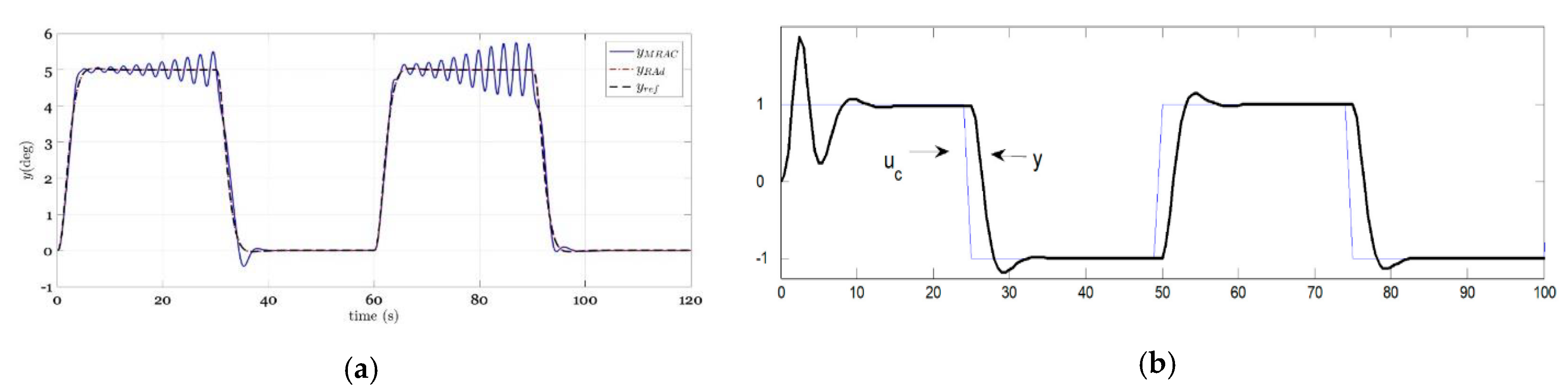
Using this established methodology, this manuscript applies the methods to control DC motors, in direct comparison with the aforementioned self-tuning methods of Åström and Wittenmark, which were already compared to one another other in 2017 [11]. This manuscript will describe the detailed development of the deterministic artificial intelligence method and subsequent application of the method to identical systems of the comparison in [11]. The demanded trajectory was the square wave, similar to that used in [11], which was illustrated in 2020 by Chen et al. [31], in order to remain challenging for nonlinear adaptive methods. This is displayed in Figure 1a, accompanied by a similar plot from [11] which establishes context for this manuscript. The research questions addressed include:
- Can deterministic artificial intelligence (D.A.I.) be successfully applied to DC motors as has recently been accomplished in spacecraft and unmanned underwater vehicles?
- How does the control of DC motors with D.A.I. compare to the performance of indirect and direct self-tuning regulators (with variations of modeling to include plant cancellations and disparate pole excesses)?
- Can implementation of D.A.I. aid target tracking of challenging square wave trajectories superior to the cited nonlinear adaptive control techniques (self-tuning regulators and model-reference adaptive controllers)?
2. Materials and Methods
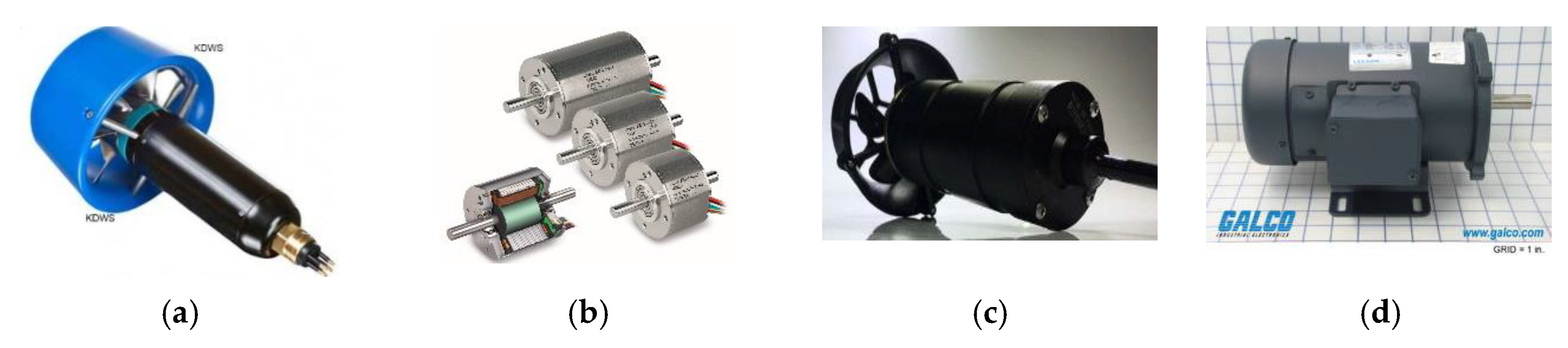
Direct current (DC) motors are common actuators for moving control surfaces on unmanned underwater vehicles (depicted in Figure 2). Motor control is a robust, well-known discipline, with state-of-the-art techniques that include nonlinear adaptive methods (e.g., self-tuning regulators and model-reference adaptive controllers) that are currently being investigated for efficacy of inclusion of artificial intelligence methods.
2.1. DC Motor Modeling
The model of the DC motor used here is taken from [8] in discrete form seen in Equation (1), which may be expressed as the difference equation seen in Equation (2).
2.2. Analytic (Autonomous) Trajectory Generation
Baker et al. [26] compared four disparate methods to develop analytic, autonomous trajectories mimicking the discontinuous step function:
- MATLAB’s Sine Function
- 4th Order Taylor Series Approximation
- Low Precision Approximation Algorithm
- High Precision Approximation Algorithm
Meanwhile, Smeresky et al. [27] adopted the first (MATLAB’s sine function) to mimic the discontinuous step function. The comparison presented in this research utilized a ubiquitous square wave, mimicked piecewise continuously by the sine function (Equations (9)–(11) in reference [26] and Figure 3 in [28]).
2.3. Deterministic A.I.: Self-Awareness Statements Using Analytic Trajectory and Optimal Learning
Shift Equation (2) to isolate u(t), establishing the form of the relationship embodying self-awareness assertion (Equations (3)–(6)). Restrict the system to only respond in accordance with the self-awareness statement—i.e., formulate u(t)) in accordance with Equation (7), defining it as , which may be expressed in regression form as the product of a matrix of knowns and a vector of unknowns, thus completing the first step: modeling. The second step (estimation) uses nominal algorithms based on recursive least squares algorithms, where the presence of the innovations or residuals indicate augmentation of recursive least squares as extended least squares. Equation (3) shifts the time index of Equation (2) to emphasis the calculation of the control—u at time t—after a few mathematical steps. This leads to Equation (8): the optimal control in feedforward form, annotated by the asterisk, i.e., u*, which is defined by a regression form of a matrix of knowns, multiplied by a vector of unknowns, , where the vector of unknowns is initialized in Equation (9), with rough estimates known a priori.
Isolate to apply control using dynamic Equation (3):
Procedure:
- Initialize the vector of unknowns per Equation (9) to assert self-awareness Equation (7) or Equation (8) as the control, where is formulated using the desired (analytic) trajectory.
- Propagate state to in Equation (11).
- Use values of (not ) and in RLS (not presented here) to optimally estimate/learn/update , to propagate errors projected on system matrix (not ).
- Apply in Equation (7) or Equation (8) with the optimally learned estimates .
3. Results
Section 2 developed the method of deterministic artificial intelligence and cited the development of several self-tuning algorithms and comparisons between them. This section presents the results of simulation experiments comparing four disparate methods, where each method attempts to follow a challenging square wave.
- Indirect self-tuner without process zero cancellation (minimum phase plant).
- Indirect self-tuner without process zero cancellation (non-minimum phase plant model assumed).
- Direct self-tuner with filtering (all process zeros cancelled).
- Deterministic artificial intelligence.
3.1. Indirect Self-Tuner without Process Zero Cancellation (Minimum Phase Plant)
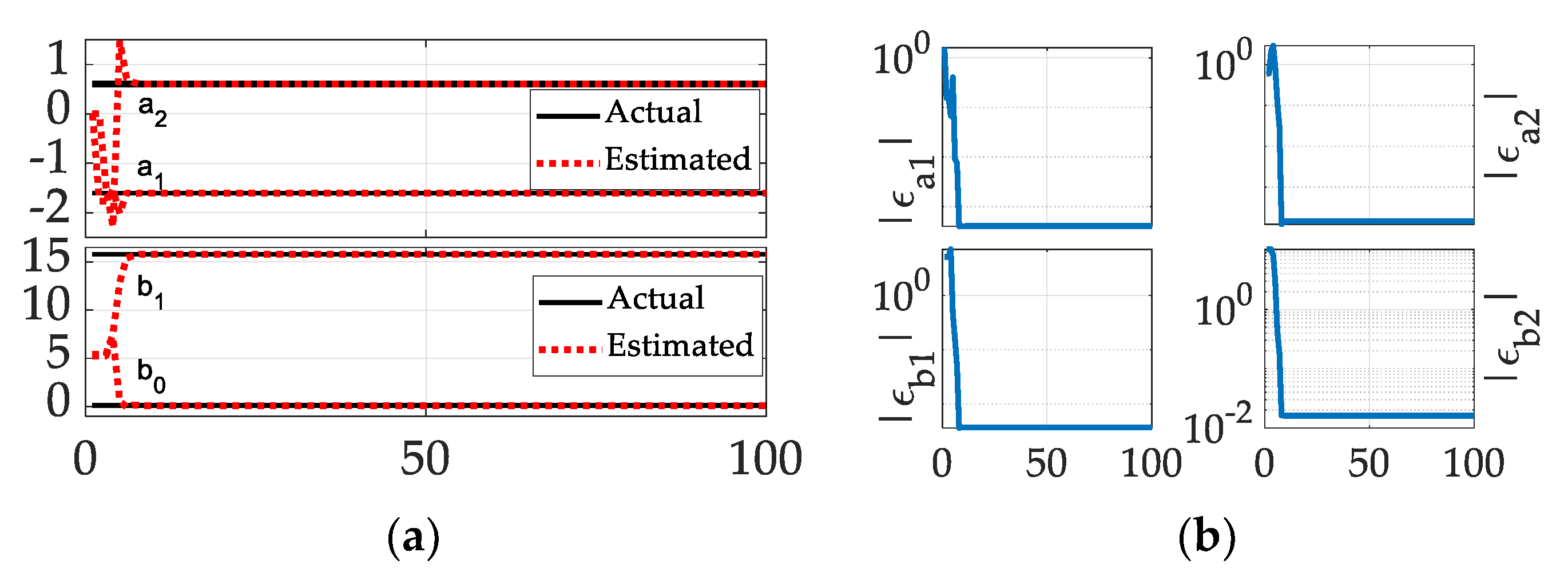
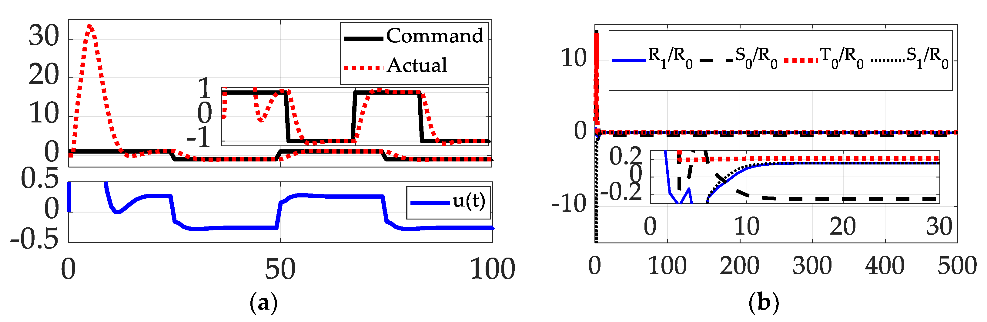
Minimum degree pole placement is presented as Algorithm 3.1 of reference [8], illustrated by example as model-following with zero cancellation (not utilized in this study) and also model-following without cancellation of process zeros (utilized here). Since the DC motor discretizes to a second order process, the minimum degree solution of polynomials R, S, and T in the control law are of first order, making the closed-loop system third order. Since no zero is cancelled, the compatibility condition (p. 95, [8]) demands that the model must have the same zero as the process. Parameters estimated by the recursive least squares family of methods are used to analytically determine coefficients of R, S, and T presented in [8] (p. 99).
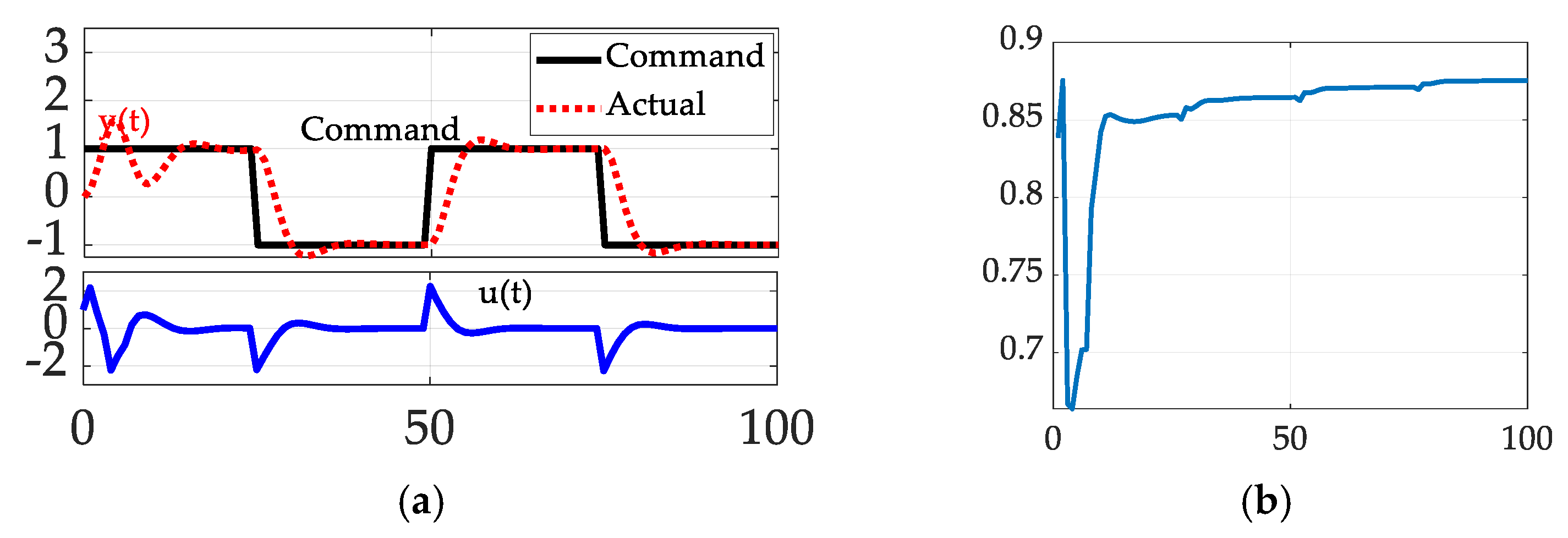
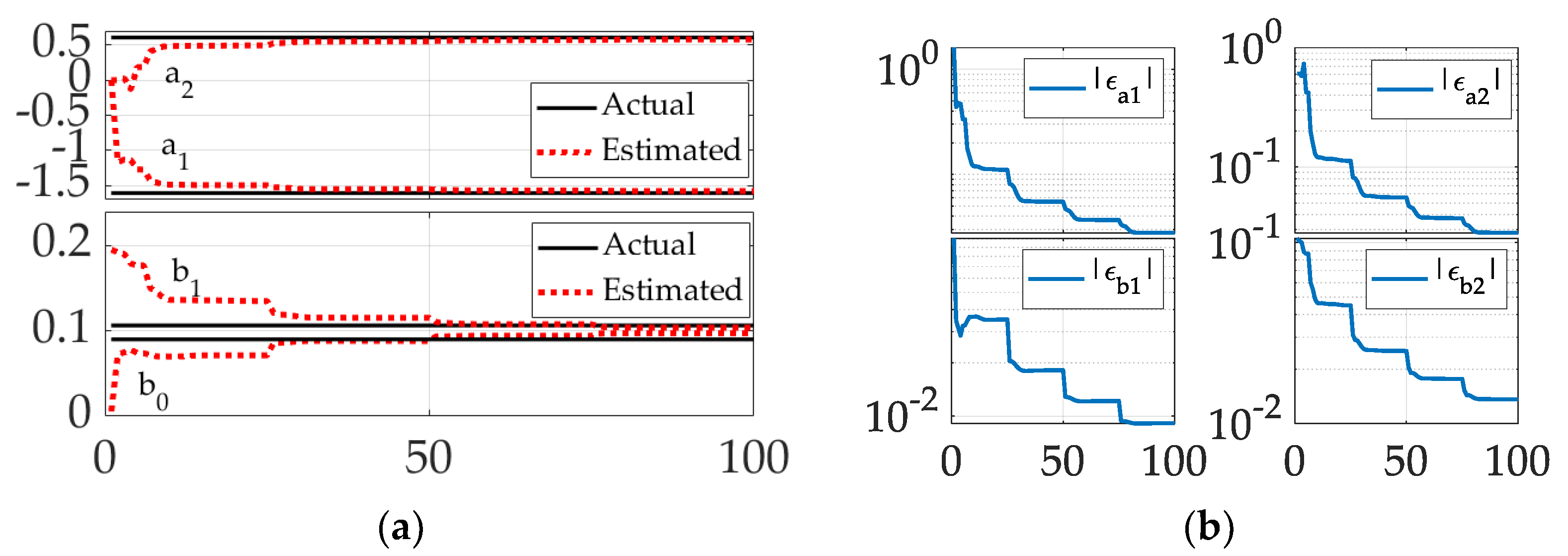
The nonlinear adaptive indirect self-tuner was used without process zero cancellation to follow a square wave, assuming a minimum phase plant; the results are displayed in Figure 3 and Figure 4. Figure 3a reveals nominal performance following the square wave; the performance included the ubiquitous overshoot and settling behavior at each switch of the square wave. The gain term oscillated very briefly, and then converged toward a steady-state value, displayed in Figure 3b. Figure 4a displays estimation by recursive least squares, while Figure 4b displays extended least squares’ attempts to estimate the residuals.
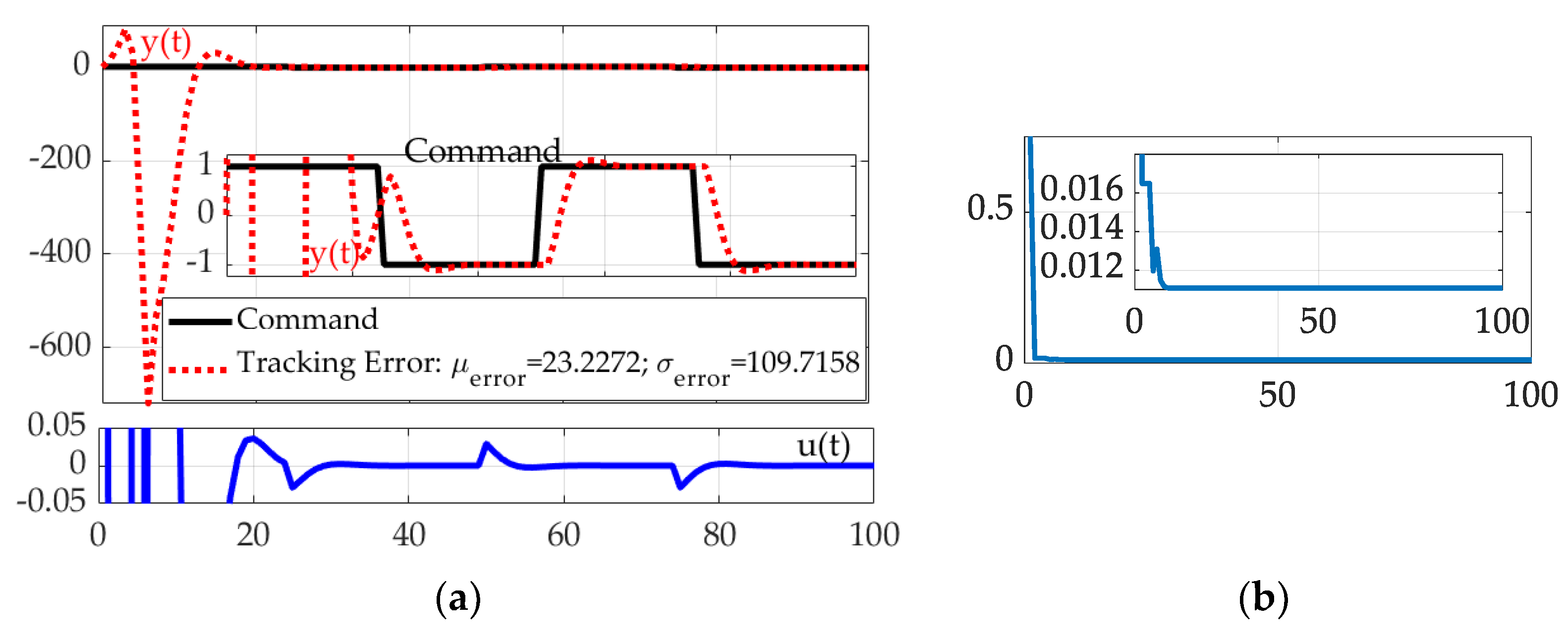
3.2. Indirect Self-Tuner without Process Zero Cancellation (Non-Minimum Phase Plant Model Assumed)
Minimum degree pole placement combined with versions of recursive least squares established the definition of a self-tuning regulator used in this study. While Section 3.1 displayed the results of indirect self-tuners without cancellation of process, this section displays the results of using an indirect self-tuner that seeks cancellation of a process zero, assuming a non-minimum phase plant. The parameters of the model shared the same structure as in Section 3.1, but the control law included cancellation of process zero.
Figure 5a reveals nominal performance following the square wave, and the performance included the ubiquitous overshoot and settling behavior at each switch of the square wave. The (not depicted) discrete control signal produced “ringing” in the control with a period of two sampling periods, while the continuous version zeros (as derived in Section 3.4 of [8]) displayed in Figure 5a eliminated ringing but retained the characteristic overshoot and settling behavior at each switch of the square wave. Relative to the earlier presented instance of no zero cancellation, Figure 5b reveals essentially no oscillation amidst convergence towards steady-state gain. Figure 6a displays estimation by least squares, while Figure 6b displays extended least squares’ attempts to estimate the residuals.
3.3. Direct Self-Tuner with Filtering (All Process Zeros Cancelled)
Due to the cumbersome design mathematics associated with indirect algorithms, direct self-tuners seek to reduce or eliminate such calculations by reparametrizing the model in terms of the parameters of the controller. The procedure is very well described in Section 3.5 of [8]. The procedure utilizes the Diophantine equation to partition the reparameterization into the following list:
- Terms in denominator polynomial A to be found by the estimator.
- Remaining terms of denominator polynomial A.
- Terms left over after factoring numerator polynomial .
- Gain term plus terms we can’t cancel in numerator polynomial B.
- Output polynomial of the controller.
The Diophantine equation can be considered a process model that is parameterized in the coefficients of polynomials , , and , so the control law is obtained directly upon parameter estimation without any design efforts. The presence of this term on the right-hand side of the Diophantine equation makes the model nonlinear in the parameters (foreshadowing nonoptimality using least squares). Seeking to avoid this difficulty often leads to the implementation of the special case of constant indicating minimum phase systems, but this workaround still cancels poorly damped zeros and can lead to ringing in the control signal.
3.4. Deterministic Artificial Intelligence
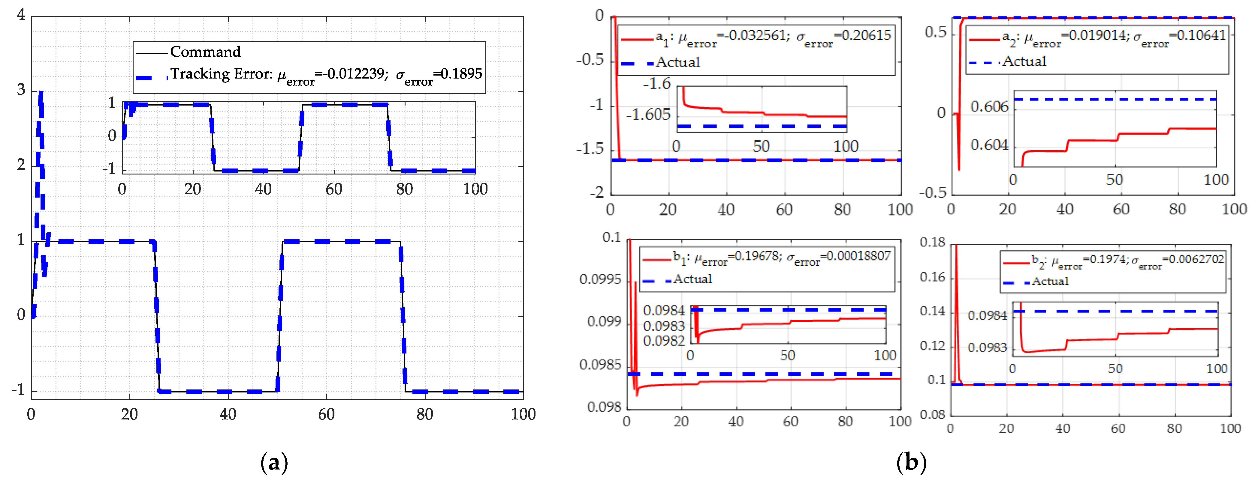
Implementing the procedure in Section 2.3 of this manuscript using the sinusoidal trajectory of Section 2.2 to mimic the steps in the square wave, Figure 8a displays an initial overshoot twice as large as in the case of the indirect self-tuner without process zero cancellation (minimum phase plant), but much less than the other cases investigated. More significantly, it appears to have eliminated the repeated overshoots and settling at each switch of the square wave.
3.5. Comparison of Estimation Accuracy
This section compiles the estimation error performance for each case investigated. Table 1 displays coefficient estimation accuracy. Little differences can be discerned between the ability of recursive least squares-based estimation of parameters with respect to mean and standard deviation of estimation errors.
3.6. Persistent Excitation
In order to contemplate whether relative performances were attributable to algorithm topology or the nature of the method to take advantage of parameter convergence, persistent excitation is briefly discussed in two theorems. These are compiled here to aid readers by assembling the disparate parts of the theorems into a few lines, as opposed to leaving them spread across many pages (particularly with respect to the proofs).
Theorem 1.
Taken from [8] (p. 64)—Persistent excitation: A signal u is called persistently exciting of order n if the limits (Equation (13)) and if the matrix given by Equation (12) is positive definite, where no mean value is included in the definition of empirical covariance c(k). Estimation is consistent and variance of the estimates goes to zero as 1/t if the input signal is persistently exciting of order n.
An alternative description of persistent excitation follows. A signal u is said to be persistently exciting of order n if for every t there exists an integer m such that Equation (14) holds.
where and the vector is given by Equation (15) permitting Equation (12) to be expressed as Equation (16).
Proof of Theorem 1
([8]). Assembled from pages 42, 48, and 65 if the parameter is chosen to minimize the least squares loss function , parameter estimates are such that Equation (17) holds. □
If matrix is nonsingular, the minimum is unique and given by (also known as the pseudo-inverse solution). Assuming data is generated by an approximated system, as in equation (18), plus independent, random noise or errors e(i) with zero mean and variance , the estimates are unbiased and converge to the true parameter value as the number of observations increases infinity, per Theorem 2.2 in [8] (p. 48).
Theorem 2
([8]). Applied to this research theorem and proof as taken from p. 65: The signal u in Equation (13) is persistently exciting of order n if and only if Equation (19) holds for all nonzero polynomials A of degree n-1 or less.
Proof of Theorem 2.
Where is defined by Equation (12) and polynomial A(q) defined by Equation (19), an uncomplicated calculation shows Equation (20) is true; if is positive definite, the right-hand side and left-hand side of equation (12) are positive for all a. □
For periodic signals u(t) of period n, it follows that , thus the signal can at most be persistently exciting of order n, the period.
3.7. Trajectory Tracking Performance Comparison
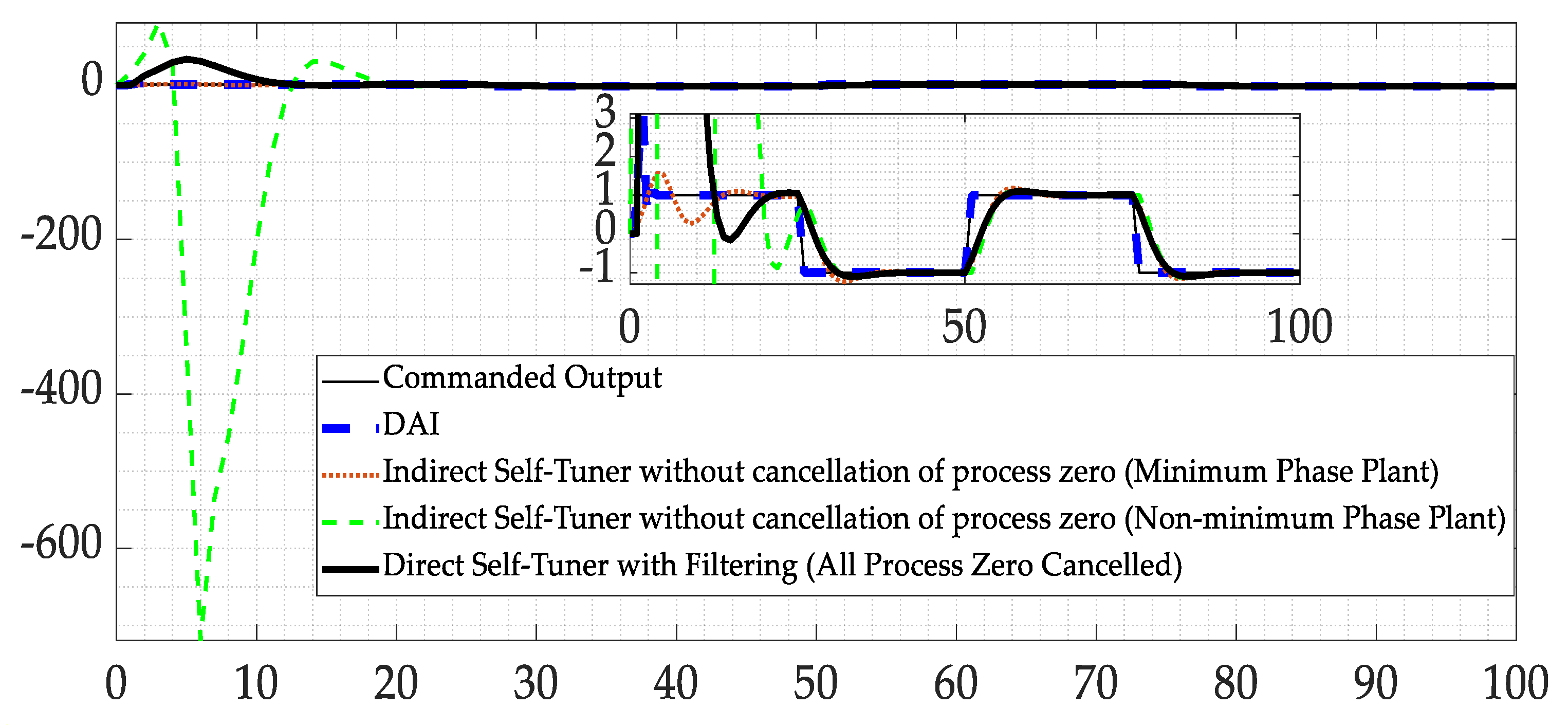
This section assembles the target tracking performances on a single multi-plot to bestow qualitative indications of relative superiority of approaches in direct comparison. Figure 9—with corresponding figures of merit in Table 2—illustrates that all methods have an initial transient associated with both the initial conditions and the initial discontinuous step to initiate the square wave. Indirect self-tuner without process zero cancellation (minimum phase plant) peaks around 1.5 while deterministic artificial intelligence peaks around 3.0. Meanwhile, both remaining methods begin with much larger transients. At each switch of the square wave, these two same methods have nearly indistinguishable performances, while slightly more overshoot is qualitatively visible for the indirect self-tuner without process zero cancellation (minimum phase plant). It is noteworthy that after the initial startup transient, deterministic artificial intelligence appears to follow the square wave without noticeable overshoot or settling.
Table 2 lists figures of merit for trajectory tracking, corresponding to the results in Figure 9. The minimum mean and standard deviation of tracking errors are highlighted with bold font indicating that deterministic artificial intelligence was superior in both categories, while very similar mean error (alone) was achieved by the indirect self-tuner without process zero cancellation (minimum phase plant).
4. Discussion
Formerly, the indirect self-tuner without process zero cancellation for minimum phase plants had superior performance (measured by mean and standard deviation) compared to the three other methods investigated, although a notable mention must go to the direct self-tuner with filtering where all process zeros are cancelled. This research qualitatively reveals deterministic artificial intelligence produces superior performance categorized by the second largest initial transient, but the transient was not repeated with each switch of the square wave like all other methods investigated. The indirect self-tuner without process zero cancellation (minimum phase plant) yielded a smaller initial transient, but the transient reoccurred with each switch of the square wave.
This research quantitatively reveals that deterministic artificial intelligence yields 4.8% lower mean and 211% lower standard deviation of tracking errors as compared to the second-best method investigated (indirect self-tuner without process zero cancellation and minimum phase plant). The improved performance cannot be attributed to superior estimation. Coefficient estimation was merely on par with the best alternative methods (some coefficients were estimated more accurately, others less accurately). Instead, the superior performance must be attributed to the method itself.
Considering the demonstrated ability to follow a challenging square wave closely in steady-state without repeated overshoots and settling after switching, future research should focus on elimination of the sole transient (on initial startup) to further improve results. Additional future research should include evaluation of the limits of uncertainty that can be autonomously counted by deterministic artificial intelligence (D.A.I.). Like the nonlinear adaptive control methods, D.A.I. is structured precisely to modify behavior in response to uncertainty and/or changes in operating conditions. Therefore, a direct comparison of each method’s ability to counter these deleterious effects would be very interesting research.
Funding
This research received no external funding.
Data Availability Statement
Data supporting reported results can be provided by contacting the author.
Acknowledgments
The inspiring genesis of this work was the following manuscript (https://0-www-mdpi-com.brum.beds.ac.uk/2077-1312/8/8/578, accessed on 25 February 2021) whose research was funded by grant money from the U.S. Office of Naval Research consortium for robotics and unmanned systems education and research described at https://calhoun.nps.edu/handle/10945/6991, accessed on 25 February 2021. The grants did not cover the costs to publish in open access, instead the author self-funds open access publication to maximize benefit to mankind.
Conflicts of Interest
The author declares no conflict of interest.
References
- Gauss, K. Theory of the Motion of the Heavenly Bodies; Dover: New York, NY, USA, 1963. [Google Scholar]
- Bierman, G. Factorization Methods for Discrete Sequential Estimation; Academic Press: New York, NY, USA, 1977. [Google Scholar]
- Kalman, R. Design of a self-optimizing control system. Trans. ASME 1958, 80, 468–478. [Google Scholar]
- Peterka, V. Adaptive digital regulation of noisy systems. In Preprints of the 2nd IFAC Symposium on Identification and Process Parameter Estimation; UTIA ČSAV: Prague, Czech Republic, 1970; p. 62. [Google Scholar]
- Wieslander, J.; Wittenmark, B. An approach to adaptive control using real time identification. Automatica 1971, 7, 211–217. [Google Scholar] [CrossRef]
- Åström, K.; Wittenmark, B. On the Control of Constant but Unknown Systems; 5th IFAC World Congress: Paris, France, 1972. [Google Scholar]
- Åström, K.; Wittenmark, B. On self-tuning regulators. Automatica 1973, 9, 185–199. [Google Scholar] [CrossRef]
- Åström, K.; Wittenmark, B. Adaptive Control; Addison-Wesley: Boston, FL, USA, 1995; pp. 43, 48, 63–65, 331. [Google Scholar]
- Slotine, J.; Weiping, L.W. Applied Nonlinear Control; Prentice-Hall: London, UK, 1991; pp. 331, 365. [Google Scholar]
- Sands, T. Space System Identification Algorithms. J. Space Explor. 2018, 6, 138. [Google Scholar]
- Sands, T. Nonlinear-Adaptive Mathematical System Identification. Computation 2017, 5, 47. [Google Scholar] [CrossRef] [Green Version]
- Rubaai, A.; Kotaru, R. Online identification and control of a DC motor using learning adaptation of neural networks. IEEE Trans. Ind. Appl. 2000, 36, 935–942. [Google Scholar] [CrossRef]
- Liu, Z.; Zhuang, X.; Wang, S. Speed Control of a DC Motor using BP Neural Networks. In Proceedings of the 2003 IEEE Conference on Control Applications, Istanbul, Turkey, 25–25 June 2003; pp. 832–835. [Google Scholar]
- Mishra, M. Speed Control of DC Motor Using Novel Neural Network Configuration. Bachelor’s Thesis, National Institute of Technology, Rourkela, India, 2009. [Google Scholar]
- Hernández-Alvarado, R.; García-Valdovinos, L.G.; Salgado-Jiménez, T.; Gómez-Espinosa, A.; Fonseca-Navarro, F. Neural Network-Based Self-Tuning PID Control for Underwater Vehicles. Sensors 2016, 16, 1429. [Google Scholar] [CrossRef] [PubMed] [Green Version]
- Hussein, A.; Gaber, M.M.; Elyan, E.; Jayne, C. Imitation learning: A survey of learning methods. ACM Comput. Surv. 2017, 50, 21. [Google Scholar] [CrossRef]
- Dessort, R.; Chucholowski, C. Explicit model predictive control of semi-active suspension systems using Artificial Neural Networks (ANN). In 8th International Munich Chassis Symposium 2017; Pfeffer, P.E., Ed.; Springer Fachmedien Wiesbaden: Wiesbaden, Germany, 2017; pp. 207–228. [Google Scholar]
- Wei, B. Adaptive Control Design and Stability Analysis of Robotic Manipulators. Actuators 2018, 7, 89. [Google Scholar] [CrossRef] [Green Version]
- Rashwan, A. An Indirect Self-Tuning Speed Controller Design for DC Motor Using A RLS Principle. In Proceedings of the 21st International Middle East Power Systems Conference (MEPCON), Cairo, Egypt, 17–19 December 2019; pp. 633–638. [Google Scholar]
- Cursi, F.; Mylonas, G.P.; Kormushev, P. Adaptive Kinematic Modelling for Multiobjective Control of a Redundant Surgical Robotic Tool. Robotics 2020, 9, 68. [Google Scholar] [CrossRef]
- Dengler, C.; Lohmann, B. Adjustable and Adaptive Control for an Unstable Mobile Robot Using Imitation Learning with Trajectory Optimization. Robotics 2020, 9, 29. [Google Scholar] [CrossRef]
- Li, W.; Zhang, C.; Gao, W.; Zhou, M. Neural Network Self-Tuning Control for a Piezoelectric Actuator. Sensors 2020, 20, 3342. [Google Scholar] [CrossRef] [PubMed]
- Dini, P.; Saponara, S. Design of Adaptive Controller Exploiting Learning Concepts Applied to a BLDC-Based Drive System. Energies 2020, 13, 2512. [Google Scholar] [CrossRef]
- Cooper, M.; Heidlauf, P.; Sands, T. Controlling Chaos—Forced van der Pol Equation. Mathematics 2017, 5, 70. Available online: https://0-www-mdpi-com.brum.beds.ac.uk/2227–7390/5/4/70 (accessed on 17 January 2021).
- Lobo, K.; Lang, J.; Starks, A.; Sands, T. Analysis of Deterministic Artificial Intelligence for Inertia Modifications and Orbital Disturbance. Int. J. Control Sci. Eng. 2018, 8, 53. [Google Scholar]
- Baker, K.; Cooper, M.; Heidlauf, P.; Sands, T. Autonomous trajectory generation for deterministic artificial intelligence. Electr. Electron. Eng. 2018, 8, 59. [Google Scholar]
- Smeresky, B.; Rizzo, A.; Sands, T. Optimal Learning and Self-Awareness Versus PDI. Algorithms 2020, 13, 23. [Google Scholar] [CrossRef] [Green Version]
- Sands, T. Development of deterministic artificial intelligence for unmanned underwater vehicles (UUV). J. Mar. Sci. Eng. 2020, 8, 578. [Google Scholar] [CrossRef]
- Sands, T.; Bollino, K.; Kaminer, I.; Healey, A. Autonomous Minimum Safe Distance Maintenance from Submersed Obstacles in Ocean Currents. J. Mar. Sci. Eng. 2018, 6, 98. [Google Scholar] [CrossRef] [Green Version]
- Sands, T. (Ed.) Deterministic Artificial Intelligence; IntechOpen: London, UK, 2020; ISBN 978-1-78984-111-4. [Google Scholar]
- Chen, J.; Wang, J.; Wang, W. Robust Adaptive Control for Nonlinear Aircraft System with Uncertainties. Appl. Sci. 2020, 10, 4270. [Google Scholar] [CrossRef]
- AliExpress DC Motor. Available online: https://www.aliexpress.com/item/32363144992.html (accessed on 18 January 2021).
- Unmanned Systems Technology DC Motor. Available online: https://www.unmannedsystemstechnology.com/2015/05/maxon-launches-high-torque-dc-brushless-motors/ (accessed on 18 January 2021).
- Maxon Motor EC-i 40 DC Motor. Available online: http://mymobilemms.com/OFFTHEGRIDWATER.CA/Brushless-Motor/RCD-MI50-Stuwkracht-5-Kg-Onderwater-Sub-DC-Motor-ROV-AUV (accessed on 18 January 2021).
- Galco Industries DC Motor. Available online: https://www.galco.com/buy/Leeson/108092.00?source=googleshopping&utm_source=adwords&utm_campaign=&gclid=EAIaIQobChMIvcHsn4Gm7gIVYiCtBh0eGQGGEAkYAiABEgKOxfD_BwE (accessed on 18 January 2021).
Figure 1.
Contextual preface: model-reference and self-tuning regulator adaptive controllers following square waves. (a) Context: model-reference adaptive control in [31] following a (sloped) square wave. (b) Context: indirect self-tuning regulator in [11] following a (sloped) square wave.

Figure 2.
Representative Direct Current (DC) motors used as actuators for unmanned underwater vehicles (modeled in Equations (1) and (2) as described in [8]). (a) Marine Propeller DC motor [32]. (b) Unmanned Systems Technology DC motor [33]. (c) Maxon EC-i 40 DC motor [34]. (d) Galco Industries DC Motor [35].

Figure 3.
Indirect self-tuner without process zero cancellation (minimum phase plant). (a) command and actual output (top); and control (bottom) versus number of timesteps, revealing nominal performance following the square wave. (b) Gain versus timesteps revealing brief oscillation, and then convergence towards a steady-state value.

Figure 4.
Indirect self-tuner without process zero cancellation (minimum phase plant) with timesteps on the abscissa. (a) arameter estimation. (b) Extended least squares’ estimation of the residuals or innovations.
Figure 4.
Indirect self-tuner without process zero cancellation (minimum phase plant) with timesteps on the abscissa. (a) arameter estimation. (b) Extended least squares’ estimation of the residuals or innovations.

Figure 5.
Indirect self-tuner without process zero cancellation (non-minimum phase plant) with timesteps on the abscissa. (a) Command and actual output (top); and control (bottom). (b) Gain .
Figure 5.
Indirect self-tuner without process zero cancellation (non-minimum phase plant) with timesteps on the abscissa. (a) Command and actual output (top); and control (bottom). (b) Gain .

Figure 6.
Indirect self-tuner without process zero cancellation (non-minimum phase plant) with timesteps on the abscissa. (a) Parameter estimation. (b) Extended least squares’ estimation of the residuals or innovations.
Figure 6.
Indirect self-tuner without process zero cancellation (non-minimum phase plant) with timesteps on the abscissa. (a) Parameter estimation. (b) Extended least squares’ estimation of the residuals or innovations.

Figure 7.
Direct self-tuner with filtering (all process zeros cancelled) where timesteps appear on the abscissa. (a) Command and actual output (top); and control (bottom). (b) Gain .
Figure 7.
Direct self-tuner with filtering (all process zeros cancelled) where timesteps appear on the abscissa. (a) Command and actual output (top); and control (bottom). (b) Gain .

Figure 8.
Deterministic artificial intelligence (where timesteps appear on the abscissa). (a) Command trajectory tracking by deterministic artificial intelligence with noteworthy comparable initial overshoot, but seemingly eliminating overshoot and settling at each switch of the square wave. (b) Coefficient estimation illustrating rapid convergence towards the correct coefficient value with continued convergence at very small scale with time passage.

Figure 9.
Response comparison with corresponding results in Table 2. The solid (thin) black line is the commanded square wave trajectory. Roughly coincident with this commanded trajectory (after the initial transient) appears the blue-dashed line, representing the response of deterministic artificial intelligence. The red-dotted line represents the indirect self-tuner without process zero cancellation (minimum phase plant). Indirect self-tuner without process zero cancellation (non-minimum phase plant) is represented by the dashed-green line, while the solid (thick)-black line representing direct self-tuner with filtering (all process zeros cancelled).


Table 1.
Coefficient estimation accuracy of all four methods investigated.
| Method | Estimates 1 | |||
|---|---|---|---|---|
| Indirect self-tuner without process zero cancellation (minimum phase plant) | 0.19537 | 0.1753 | ||
| −0.02096 | 0.12801 | |||
| 0.019307 | 0.01283 | |||
| −0.02905 | 0.02060 | |||
| Indirect self-tuner without process zero cancellation (non-minimum phase plant) | −0.00957 | 0.16784 | ||
| 0.051825 | 0.37542 | |||
| −0.22845 | 1.1204 | |||
| 0.42768 | 1.9589 | |||
| Direct self-tuner with filtering (all process zeros cancelled) | 0.001976 | 0.06214 | ||
| −0.03805 | 0.66009 | |||
| −0.03052 | 0.6132 | |||
| 0.039206 | 0.68119 | |||
| Deterministic artificial intelligence | −0.03256 | 0.20615 | ||
| 0.019014 | 0.10641 | |||
| 0.19678 | 0.00019 | |||
| 0.1974 | 0.00627 | |||
1 Estimation error comparison of proposed deterministic artificial intelligence (D.A.I.) method to formerly compared methods in [11].
Table 2.
Tracking errors‘ figures of merit (means and standard deviations) for each technique.
| Method | Tracking Error 1 | |
|---|---|---|
| Indirect self-tuner without process zero cancellation (minimum phase plant) | 0.023534 | 0.58929 |
| Indirect self-tuner without process zero cancellation (non-minimum phase plant) | 23.2272 | 109.7158 |
| Direct self-tuner with filtering (all process zeros cancelled) | −0.35445 | 2.9984 1 |
| Deterministic artificial intelligence (D.A.I.) | −0.012239 | 0.1895 |
1 Tracking error comparison of proposed D.A.I. method to formerly compared methods in [11].
Publisher’s Note: MDPI stays neutral with regard to jurisdictional claims in published maps and institutional affiliations. |
© 2021 by the author. Licensee MDPI, Basel, Switzerland. This article is an open access article distributed under the terms and conditions of the Creative Commons Attribution (CC BY) license (http://creativecommons.org/licenses/by/4.0/).
Share and Cite
MDPI and ACS Style
Sands, T. Control of DC Motors to Guide Unmanned Underwater Vehicles. Appl. Sci. 2021, 11, 2144. https://0-doi-org.brum.beds.ac.uk/10.3390/app11052144
AMA Style
Sands T. Control of DC Motors to Guide Unmanned Underwater Vehicles. Applied Sciences. 2021; 11(5):2144. https://0-doi-org.brum.beds.ac.uk/10.3390/app11052144
Chicago/Turabian StyleSands, Timothy. 2021. "Control of DC Motors to Guide Unmanned Underwater Vehicles" Applied Sciences 11, no. 5: 2144. https://0-doi-org.brum.beds.ac.uk/10.3390/app11052144
Note that from the first issue of 2016, this journal uses article numbers instead of page numbers. See further details here.