
Influence of Load Dynamics on Converter-Dominated Isolated Power Systems


1
INESC Technology and Science, 4099-002 Porto, Portugal
2
Faculty of Engineering, University of Porto, 4099-002 Porto, Portugal
*
Author to whom correspondence should be addressed.
Appl. Sci. 2021, 11(5), 2341; https://0-doi-org.brum.beds.ac.uk/10.3390/app11052341
Submission received: 1 February 2021
/
Revised: 26 February 2021
/
Accepted: 2 March 2021
/
Published: 6 March 2021
(This article belongs to the Special Issue Isolated Power Systems Targeting 100% Integration of Renewables)
Abstract
:The operation of isolated power systems with 100% converter-based generation requires the integration of battery energy storage systems (BESS) using grid-forming-type power converters. Under these operating conditions, load dynamics influences the network frequency and voltage following large voltage disturbances. In this sense, the inclusion of induction motor (IM) load models is required to be properly considered in BESS power converter sizing. Thus, this paper presents an extensive sensitivity analysis, demonstrating how load modeling affects the BESS power converter capacity when adopting conventional control strategies while aiming to assure the successful recovery of all IM loads following a network fault. Furthermore, this work highlights that generators with converter interfaces can actively contribute to mitigate the negative impacts resulting from IM loads following a network fault. Thereby, two distinct control strategies are proposed to be integrated in the power electronic interfaces of the available converter-based generators: one to be adopted in grid-following converters and another one suitable for grid-forming converters. The proposed control strategies provide an important contribution to consolidating insular grid codes, aiming to achieve operational scenarios accommodating 100% penetration of converter-based generation with a significative percentage of the IM load composition without resorting to a significative increase in BESS power converter sizing.
1. Introduction
Battery energy storage systems (BESS) are being installed in geographical islands with large shares of converter-interfaced renewable energy sources (CI-RES) in order to provide fast power–frequency regulation reserve. This solution contributes for mitigating the displacement of the traditional thermal-based generation units in face of CI-RES increase, as this trend significantly reduces synchronous inertia and degrades power–frequency control capabilities [1,2]. Currently, the power converter interfaces used in CI-RES and BESS are typically controlled as grid-following units, thus requiring to be installed in systems where other elements operated as voltage sources assure the definition of the voltage and frequency waveform [3]. Thus, in order to achieve operating scenarios with up to 100% RES integration, the existence of power converters with grid-forming control capabilities is mandatory. The operation of this type of converter requires an energy buffer—typically a BESS—coupled to it [4]. Recently, several works have been carried out with respect to grid-forming operation modes of power converters. The concept of the virtual synchronous machine (VSM) is a widely recognized approach which aims to emulate in a power converter the inherent operational characteristics of a synchronous machine (SM) [5,6,7,8].
In power system stability analysis, the focus is traditionally associated with power-generating unit modeling, while load models are relegated to a second plan despite recognizing their influence on network stability [9]. This becomes even more relevant when the generation system is also being tremendously modified and converter-based units become the dominant sources. In fact, different load models could lead to different system stability assessment conclusions, which might affect the network planning and operation [10]. This was emphasized in [10], where the authors stressed the importance of including induction motor (IM) load models in simulation platforms in order to best fit numerical simulation results to event recordings in large interconnected systems. The obtained results led to the conclusion that a level of 20% to 30% of IM loads is required to be considered to best fit simulation studies to the recorded events.
The emergence of power electronic interfaced loads is increasing the interest in load modeling and parametrization. Within the scope of a CIGRE working group [9], the authors presented the results of a survey addressing load modeling practices in more than 160 utilities and system operators. It was concluded that, while for steady state studies there is a dominant load model type used by the inquired utilities, for the case of dynamic power system studies, no clear trend regarding the adopted models was able to be clearly identified.
A load model stablishes the mathematical representation of the relationship between its active and reactive power response with respect to time and/or grid quantities (in particular, frequency and voltage). The load models can be generally divided into two main categories: static and dynamic. Static load models express their active and reactive powers in any instant of time as functions of the bus voltage and frequency, with ZIP and exponential models being typical implementations associated to this category. The dynamic load models express the time dependence of active and reactive powers, being generally represented by IM load or exponential recovery load models [11]. There are two distinct approaches for identifying the load model parameters: measurement-based and component-based. The component-based method consists of the knowledge of physical behaviors of loads. However, such information is not always possible to obtain. On the other side, the measurement-based method consists in collecting a measurement’s dataset which is used to identify the load model parameters that best suit the measurement data [11]. More recently, distinct load modeling strategies have been proposed in the literature. Composite load models consist in a combination of static and dynamic load models, and some authors state that these models could provide more accurate responses [11,12]. An alternative method to modeling nonlinear loads consists in taking advantage of artificial neural networks for load representations under a black-box modeling approach. This method perceives the system behavior without the need for a physical model to calculate the output [11,13]. With the wide development of the smart grid concept, the need for developing load models with the ability of incorporating the changes in power consumption in response to the customer behavior also emerged. Therefore, some authors proposed load models which incorporate the impact of demand side management. Such models are designed based on their physical characteristics and can be controlled to reflect the desired demand response strategy [11,14]. In recent years, due to large-scale integration of distributed generation in distribution grids, some authors focused on developing aggregated models of active distribution networks in the face of the transmission grid exploiting “black-box” and “gray-box” approaches. In “black-box” modeling, the physical structure of the equivalent model is not considered, contrarily to the “gray-box” approach [11,15]. In [15], the authors proposed a “gray-box” aggregated dynamic model for active distribution networks, which is composed of an equivalent power converter, an equivalent synchronous generation unit and an equivalent load model. The aim of the proposed model is to represent the transient behavior of the distribution network following large voltage disturbances.
Recent works available in the literature addressing the impacts of load modeling lie within the scope of microgrids (MG) [16,17,18,19,20]. The relevance of proper load modeling in MG dynamics following events such as switching operations, loss of generating units and the starting of IM is discussed in [16]. In [17] the authors investigated the influence of IM in the stability of an islanded MG dominated by converter-based generation, in contrast to a case where the load is represented by static models. The authors conclude that the inclusion of IM in load modeling is of major importance to assess the network oscillatory behavior and the load margin with adequate accuracy. A similar study was performed in [18], where the stability of an islanded MG with both static and dynamic load models was analyzed. It was concluded that the interaction between the two types of loads may lead to unstable conditions. In [19], the stability of medium-voltage megawatt scale MG with IM loads was studied, and they operated with 100% converter-interfaced generation. In order to eliminate the oscillatory behavior induced by the IM loads, a damping control loop was proposed to be added to the well-known droop-controlled MG. Regarding the dynamic stability, an analysis was performed in [20] aiming to evaluate the load composition and parametrization effect, considering both static and dynamic loads. The case study consisted in a medium-voltage MG, where a fault followed by an unpredicted islanding event was considered (a slight voltage drop of 0.2 p.u. was simulated). In such conditions, the authors concluded that increasing the share of IM loads has a beneficial effect due to their inertia, thus contributing to improving the frequency behavior in the moments subsequent to the islanding. A methodology for the real-time identification of the exponential dynamic load model parameters based in real data measurement was proposed in [21]. The proposed real-time estimation of exponential load parameters is preferred in comparison with the aggregate load model (augmented with IM loads) as the number of parameters to be identified precludes real-time application.
The transient response of individual loads can directly impact the frequency and voltage stability of systems with low or non-inexistent synchronous inertia. The occurrence of short circuits in networks operating with a high percentage of constant torque IM could lead to a delayed voltage recovery due to the IM stalling. In such cases, the stalled IM will draw a large amount of reactive power from the network (five to six times its steady-state reactive power regime), precluding successful voltage recovery [22]. The specific effects resulting from the load dynamic behavior in the network transient stability must be taken into account. Nonetheless, the works presented in [16,17,18,19,20,21] do not address the relevance of this specific issue, particularly in converter-dominated systems where grid-forming-type converters have a major role.
In this paper, the operation of an isolated power system with 100% converter-based renewable generation is addressed, where a BESS connected to the grid with a grid-forming-type power converter is responsible for providing voltage and frequency regulation capabilities. Regarding the load modeling, exponential and IM load model types are considered as representative of the main loads’ dynamics, in line with recent works such as [11] and [20], while also evidencing scenarios where IM-type loads still have a high relevance in global load composition. BESS power converter sizing usually neglects loads dynamics [23,24]. However, it is demonstrated that different factors associated with dynamic load modeling largely affect the need for oversizing its power capacity when conventional control solutions are adopted in these units. This is of high relevance in order to assure the successful recovery of all of the IM load following a network fault, since it is recognized as the most severe frequency stability contingency in converter-dominated and isolated systems [25]. On the other hand, voltage-sensitive (active and reactive) current injection during faults has been pointed out as a fundamental requirement in isolated systems with high penetration of CI-RES [26]. In this work it is shown that such requirements are not suitable for specific network operating scenarios with high shares of IM loads.
Emerging from the identified gaps in the literature survey, two novel control strategies are proposed to be integrated in the power electronic interfaces of the available converter-based generators in order to support the successful recovery of IM loads following a network fault. The first approach consists of implementing an appropriate voltage/reactive current control strategy at the CI-RES (operating as grid-following units) during faults. The second approach consists of a dynamic modulation strategy for the reference voltage of the grid-forming unit during the post-fault recovery period. Both strategies intend to increase the electromagnetic torque of the IM loads during the post-fault period and hence contribute to its reacceleration. Finally, it is shown that the coordinated implementation of these two control solutions is beneficial in operating scenarios with very large shares of IM loads. It is worth noting that the positive relevance of the contribution of this work is naturally more notable as far as the share of IM load increase. In cases with a low share of IM loads, the need for the proposed solution is less relevant but still does not jeopardize system dynamics.
2. Isolated Power System Modeling
2.1. Grid-Forming Operation of Power Converters
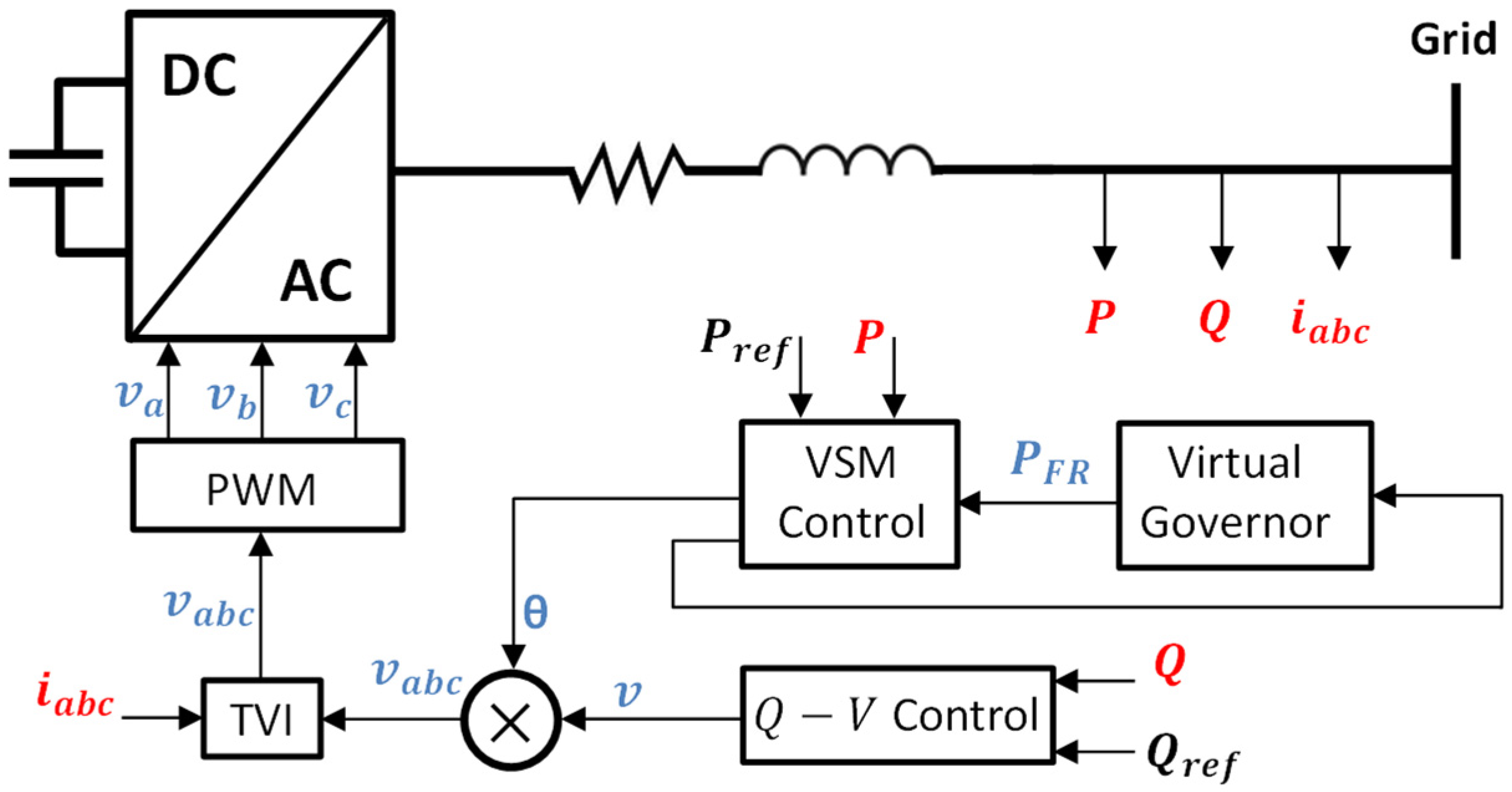
In this work, the VSM-type control approach for BESS power converter interfaces was adopted since it has been recognized as an effective solution for providing virtual inertia and damping to the power system [5,6,7]. A simplified modeling approach was adopted for the VSM operating in the grid-forming mode, which recalls the principles of the swing equation with damping and inertia [5]. A general overview of the implemented dynamic model is presented in Figure 1, including the main control blocks that are described in the next subsections being also identified.
2.1.1. Virtual Synchronous Machine Control
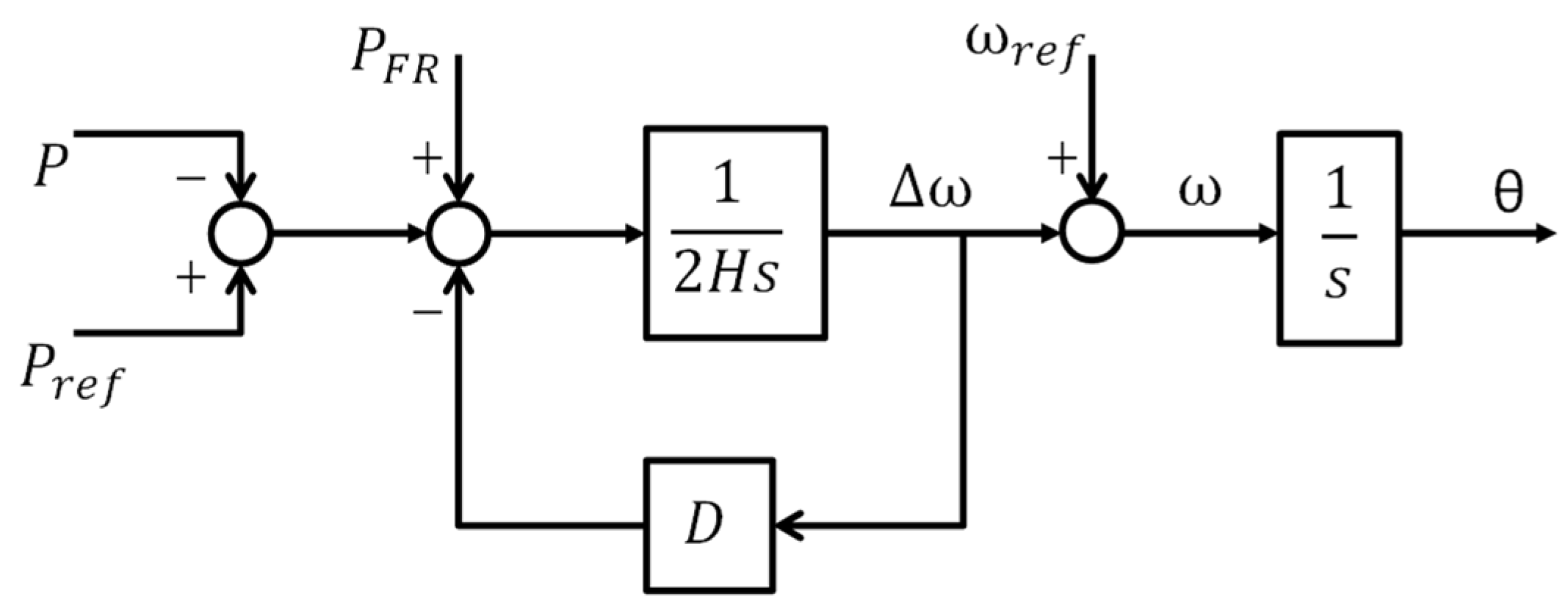
VSM control (represented by the “VSM Control” block depicted in Figure 1) corresponds to a control feature that intends to emulate the main dynamics of a SM, which is represented in a simplified manner by the swing equation. Therefore, the grid-forming voltage angle/angular frequency is synthetized based on the virtual SM swing equation. Assuming that the angular frequency can be approximated to its nominal value, the corresponding mathematical formulation (in per unit) for the swing equation is given by
where is the angular velocity of the virtual rotor, H corresponds to the inertia constant, D is the damping coefficient and and are the mechanical and electric output powers, respectively. A block diagram illustrating VSM control is presented in Figure 2, where corresponds to the active power measured at the converter point of common coupling (equivalent to ), corresponds to the active power reference setpoint and corresponds to the active power modulation given by the virtual frequency governor (described in Section 2.1.2). Note that is equivalent to the sum of and . and θ are the outputs of the controller and correspond to the angular frequency and phase angle synthetized by the converter control mechanism, i.e., the frequency and phase calculated by the VSM control loop, where is the reference value of the virtual angular frequency.
2.1.2. Virtual Speed Governor
The virtual speed governor (represented by the “Virtual Governor” block in Figure 1) corresponds to a control feature emulating the frequency regulation provided by the load frequency control mechanism existing in the SM, namely, the primary frequency control, as follows:
where corresponds to the active power modulation term as a function of the virtual angular velocity error and is the droop gain.
2.1.3. Reactive Power–Voltage Control
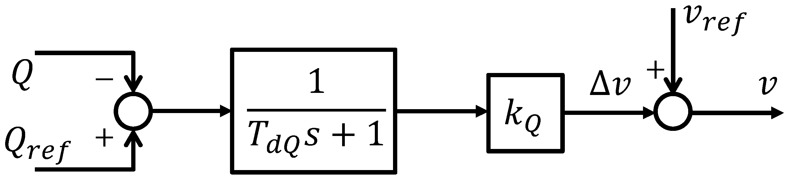
Reactive power–voltage control (represented by the “Q–V Control” block depicted in Figure 1) is responsible for defining the converter voltage magnitude as a function of the reactive power—Figure 3. Thus, and are the reference and the measured reactive power values, respectively, is the control loop time constant, is the reactive power–voltage droop control gain and and are the voltage reference and the amplitude of the output voltage to be synthetized by the converter interface.
2.1.4. Transient Virtual Impedance
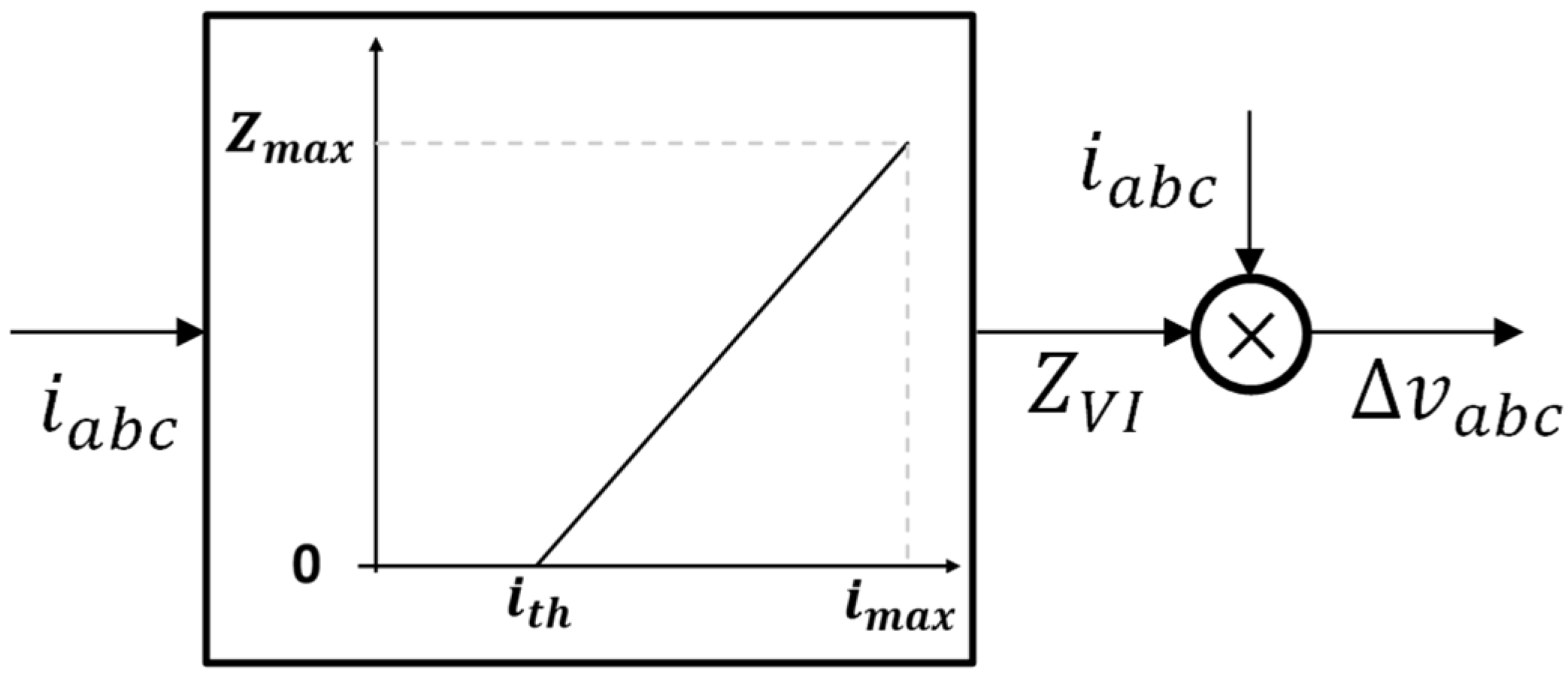
Converter interfaces typically do not have a large overcurrent capability, contrarily to conventional SM, which are able to provide large short-circuit currents [27,28]. With respect to converter interfaces operating in the grid-forming mode, current control during voltage sags is a challenging task as the current is only limited by the impedance seen at the converter terminals. In order to properly control the grid-forming converter output current during grid faults, an adequate current-limiting strategy is required. For this purpose, transient virtual impedance (TVI) was adopted, consisting in a virtual impedance at the output of the converter that is modulated as a function of the output current, aiming to achieve appropriated current limitation during grid faults [28,29]. Therefore, in case of an overcurrent, a virtual voltage drop effect will be included in the calculated voltage reference, which will represent the voltage across the virtual impedance, as follows:
where is the converter voltage reference, is the compensated voltage amplitude to be synthetized by the converter interface and represents the voltage drop across the virtual impedance, which is zero when the current magnitude is lower than a predefined threshold value, being given by:
where i corresponds to the converter output current, and and correspond to the virtual resistance and reactance, respectively. In order to achieve a smooth transition between states, i.e., between the normal and the current-limiting control mode, as soon as the current amplitude exceeds the predefined threshold value (), which is considered to be equal to the nominal current of the converter interface, the virtual impedance will present a linear increase depending on the current magnitude value. This is presented in Figure 4, where the impedance reaches the maximum value () at the maximum admissible current magnitude ().
2.2. Modeling of CI-RES Generation
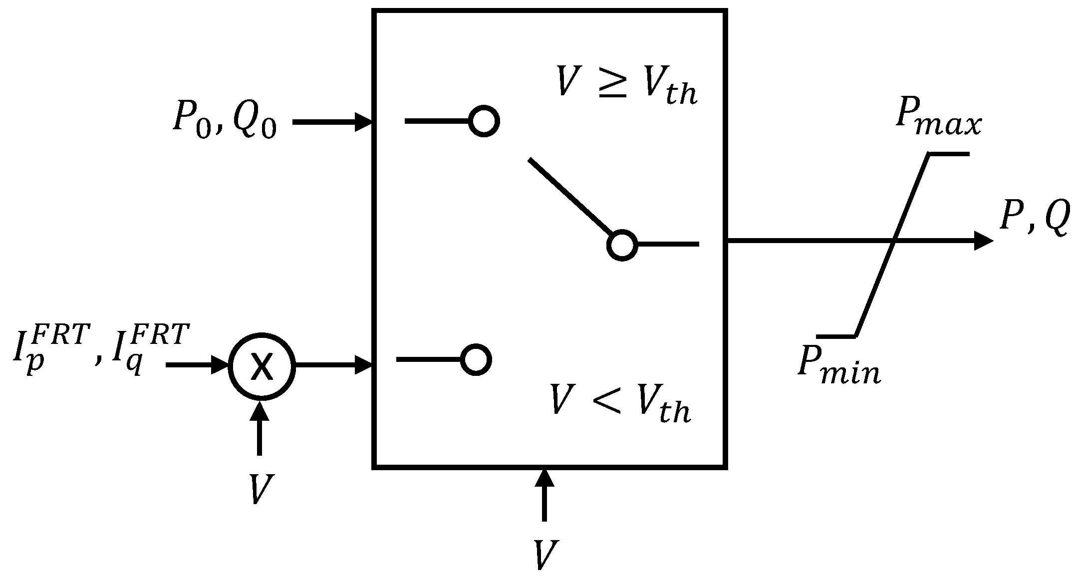
With respect to CI-RES modeling, a simplified grid-following model proposed in [30] was adopted both for wind and PV generators, which is based on a first-order transfer function approximation of the real dynamic response as well as the converter current limits. The model is endowed with fault ride through (FRT) capability, as shown in Figure 5. During normal operation conditions, and correspond to the active and reactive power setpoints (a unitary power factor was assumed). However, for voltage dips lower than , the CI-RES generators will adjust their output power according to the active () and reactive () current requirements usually defined in grid codes. In this case, is calculated proportionally to the terminal voltage deviation (a voltage dead-band of 0.15 p.u. was considered, with the current setpoint being set to 1 when the terminal voltage reaches 0.5 p.u.). Complementarily, the active current is given by:
where corresponds to the CI-RES nominal current. The CI-RES output power is bounded to its maximum ( and minimum ( limits.
2.3. Load Modeling
In this work, it was considered that the isolated power system was constituted with two main load groups: static and dynamic load models, as described in the next subsections.
2.3.1. Static Load Models
Within the static load representation, two modeling options were considered: the constant impedance and the exponential model. In both approaches, there is a voltage dependency of the load characteristics. Regarding the constant impedance load model, the active (P) and reactive (Q) power consumptions are expressed by (6) and (7), respectively, where and correspond to the nominal active and reactive power consumptions, while and are the terminal and nominal load voltages. On the other hand, in the exponential load model, active and reactive power consumptions are expressed by (8) and (9), where and are the exponential load model coefficients for the active and reactive power consumptions, which define the power consumption variation as a function of the load terminal voltage.
2.3.2. Dynamic Load Model
The dynamic loads were represented by the IM model, since it is the most common approach used in the literature [9]. The stator windings of an IM operate similarly to those of an SM, producing a magnetic field rotating at a synchronous speed. Its distinctive feature is that the rotor crents are obtained by an electromagnetic induction from the stator. In order to develop a positive torque, the rotor speed must be less than the synchronous speed:
where is the rotor angular velocity, is the stator field angular velocity and s is the slip speed of the rotor. The IM equation of motion in per unit is expressed by (11), where is the motor inertia constant, while and are the mechanical and electromagnetic torques, respectively. In this work, the implemented IM model was the one available in the MATLAB/Simulink® library, whose electrical part was represented by the fourth-order state space model, while the mechanical part was represented by a second-order model, with the rotor angle equation being expressed by (12), where is the electrical rotor angle position.
It is considered that the IM operates with constant torque at around 90% of its rated value. In addition, it was considered that each IM load is composed of three different classes: refrigerators, and small and large industrial motors (the parametrization of each IM load class is expressed in Table A1 [31]).
3. Case Study
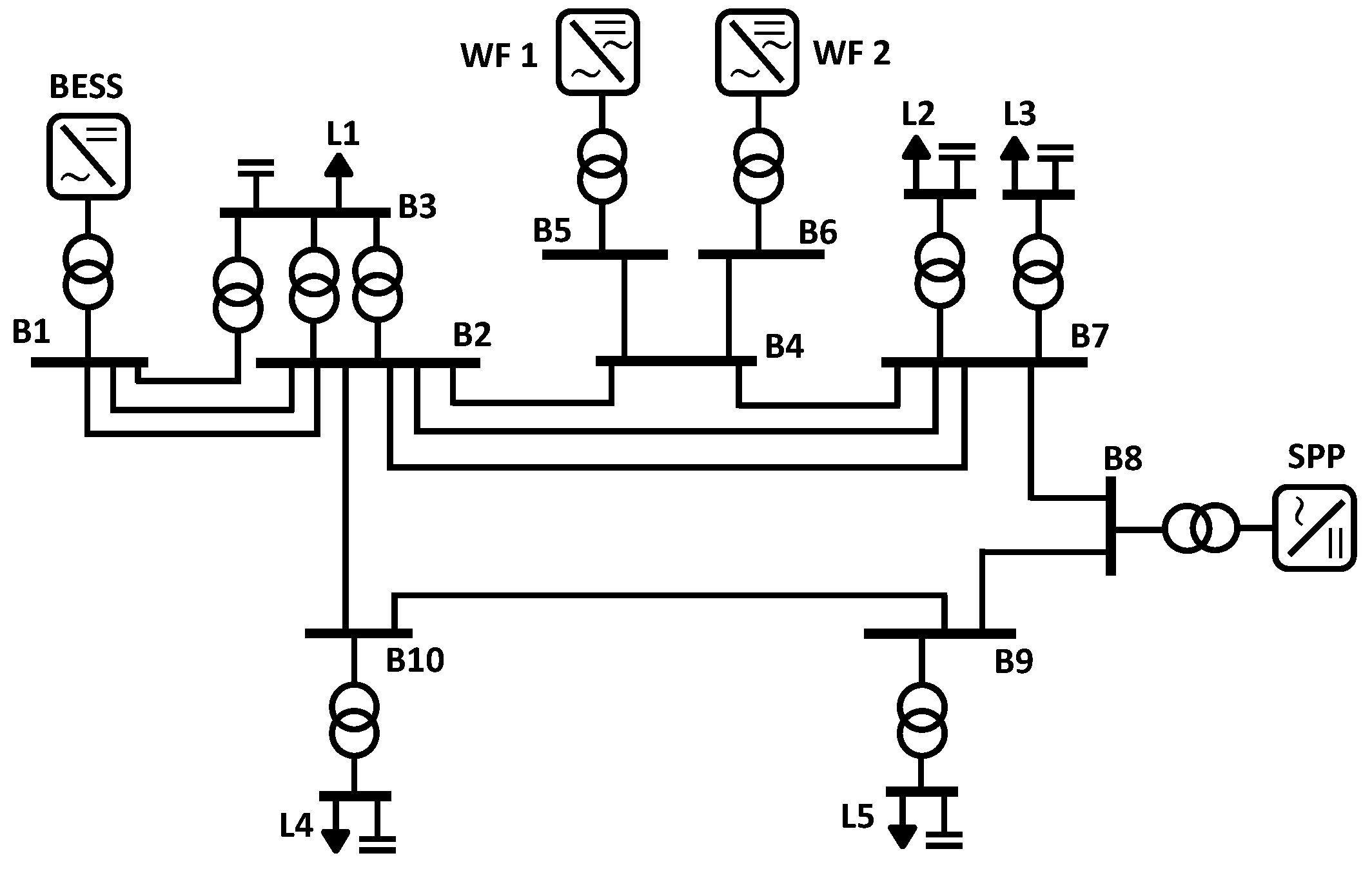
The power system of a medium-size island is considered in this paper, as shown in Figure 6, comprising a transmission infrastructure operated at 30 kV. This case study is based on a real isolated power system from a medium-size geographical island located in the European Atlantic Ocean, which was also used in previous works [30]. The data of this study case can be obtained upon request. The generation system integrates a 9 MW solar power plant (SPP) and two wind farms (WF) with a nominal power capacity of 9 (WF1) and 5.5 MW (WF2), respectively. Since the purpose of this work is to study operational scenarios with 100% converter-based generation, no thermal power plant was considered. Consequently, the local system operator assumes the integration of a BESS, whose power converter is operated as a grid-forming unit, to provide grid regulation services (for voltage and frequency). The BESS must have a power capacity which assures the system stability following large voltage disturbances (energy capacity sizing is out of the scope of this paper).
The considered network operational scenario is presented in Table 1, where CB represents capacitor banks. The admissible frequency for the system is within the range of 48.5 to 53 Hz. For frequency values below 48.5 Hz, load shedding protection takes place.
A 100 ms three-phase symmetrical short circuit occurring at t = 0 s of the simulation time in the transmission line interconnecting buses and (see Figure 6) is considered, leading to the disconnection of the line after the fault clearance. In this paper, it is intended to further develop the work presented in [32], which led to the definition of a 12 MVA BESS, due to the need for assuring N-1 generation unit tripping for the presented network operational scenarios. Based on this assumption, it is considered that the initial BESS sizing should be of at least 12 MVA. The criterion followed to define the BESS power sizing is based on the assumption that all the network elements must recover to their pre-fault state after the fault clearance.
The default grid-forming control parameters are provided in Table A2 (in Appendix A), with a maximum admissible value of the grid-forming converter interface current of 2 p.u. having been assumed, in line with some of the currently available commercial solutions [4]. Since there are no SMs operating the network, it is considered that the network frequency corresponds to the frequency synthetized by the grid-forming BESS.
4. Load Modeling Influence on Grid Dynamics
This section presents an analysis regarding the influence of the adopted load modeling on the isolated power system dynamic performance following a reference disturbance consisting of a 100 ms three-phase fault. Therefore, an extensive sensitivity analysis is presented, demonstrating how different load models, compositions and parametrizations affect the BESS power converter sizing.
4.1. Static Load Modeling—Sensitivity Analysis
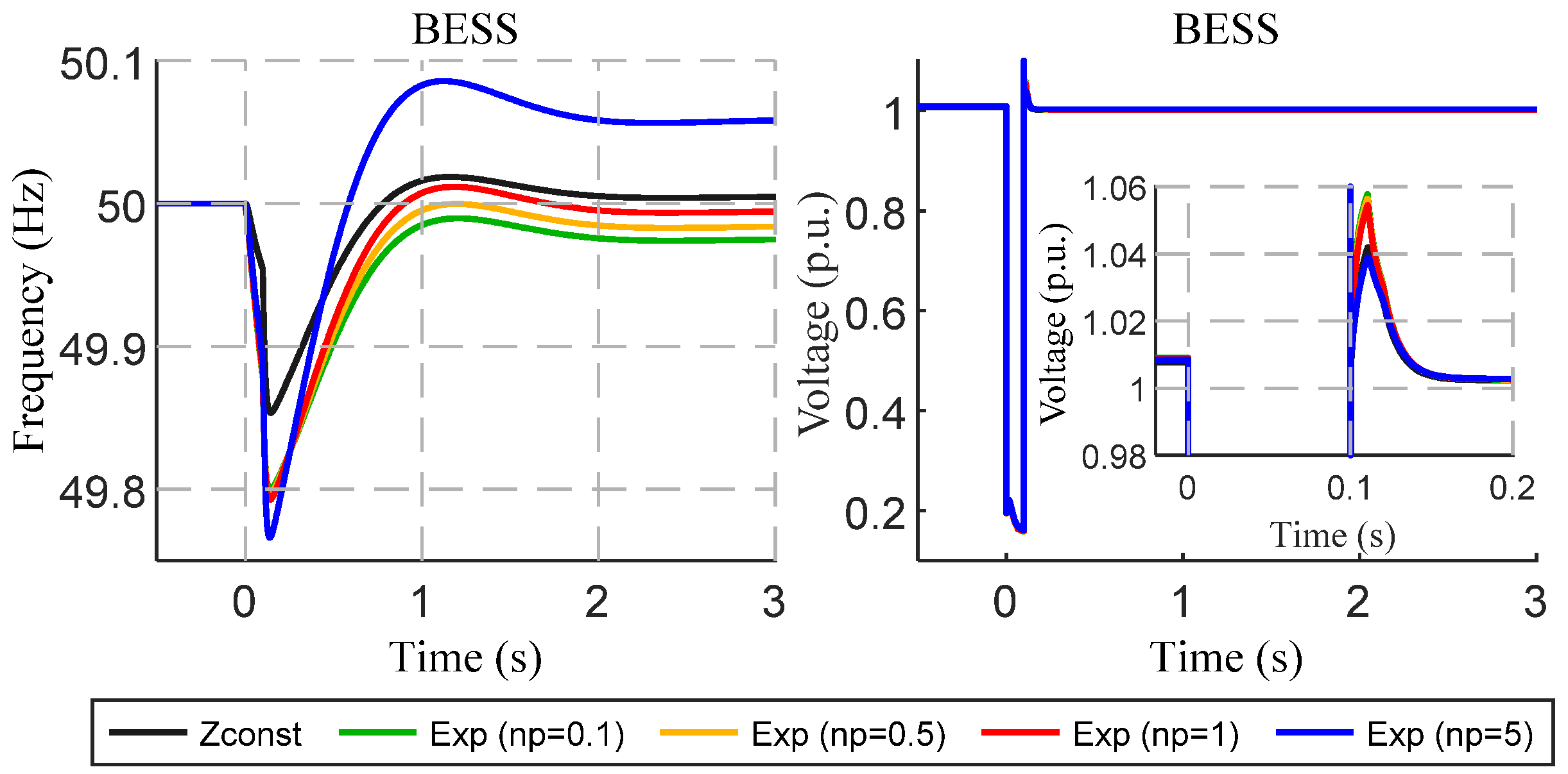
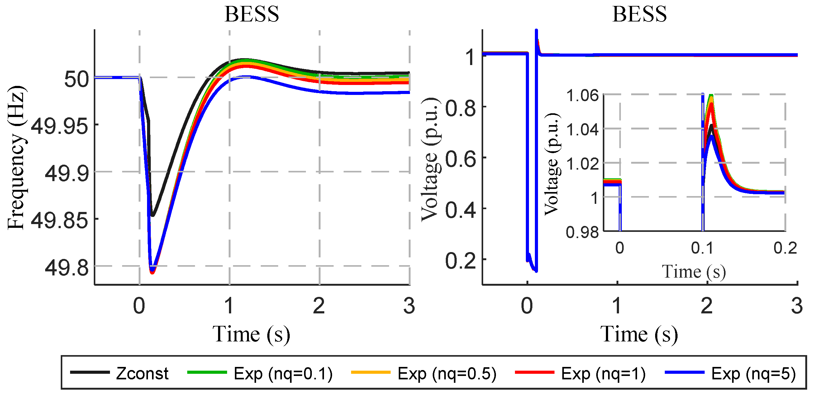
This section presents a sensitivity analysis with respect to the grid dynamics considering static load modeling. Thus, two distinct load models were analyzed: constant impedance and exponential load models. The results of the corresponding analysis are presented in Figure 7 and Figure 8. In both figures, the network frequency behavior for the cases where all the network loads are represented by constant impedance load models (Zconst) and exponential load models (Exp) is compared. However, in Figure 7, a sensitivity analysis is presented regarding the exponential model active power consumption coefficient ( value was fixed to 1), while in Figure 8, the same analysis was performed for the reactive power consumption coefficient ( value was fixed to 1). From the obtained results, it can be concluded that the variation in the exponential load model coefficients has a limited impact on the network dynamic behavior. Moreover, all the considered test cases present a smooth frequency recovery, returning to its nominal value approximately 1 s after the fault clearance.
4.2. Static and Dynamic Load Modeling—Sensitivity Analysis
In this section, it is intended to assess the impact of dynamic loads on the BESS power converter sizing. Thus, it was considered that the network load was modeled with both static and dynamic models (presented in Section 2.3). It was also considered that the IM load power consumption was evenly distributed among three different IM load types (33.3% share for each type). The following subsections present the results of an extensive sensitivity analysis regarding the IM load percentage, parametrization and composition, as well as the fault duration.
4.2.1. Base Case
The network load distribution of the base case scenario can be observed in Table 2, where it is considered that the IM loads account for 26.5% of the total system load. Regarding the loads modeled by the exponential model, the value of its power coefficients was considered equal to 1.
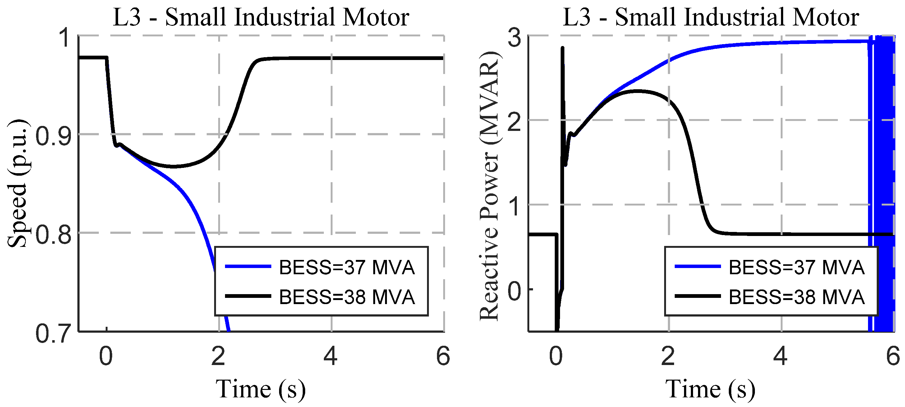
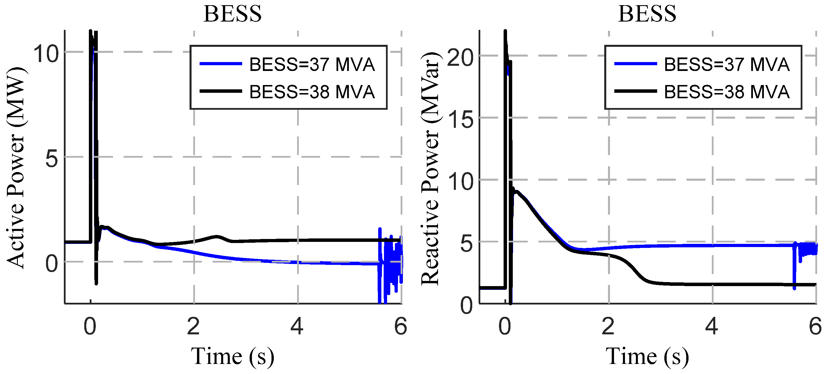
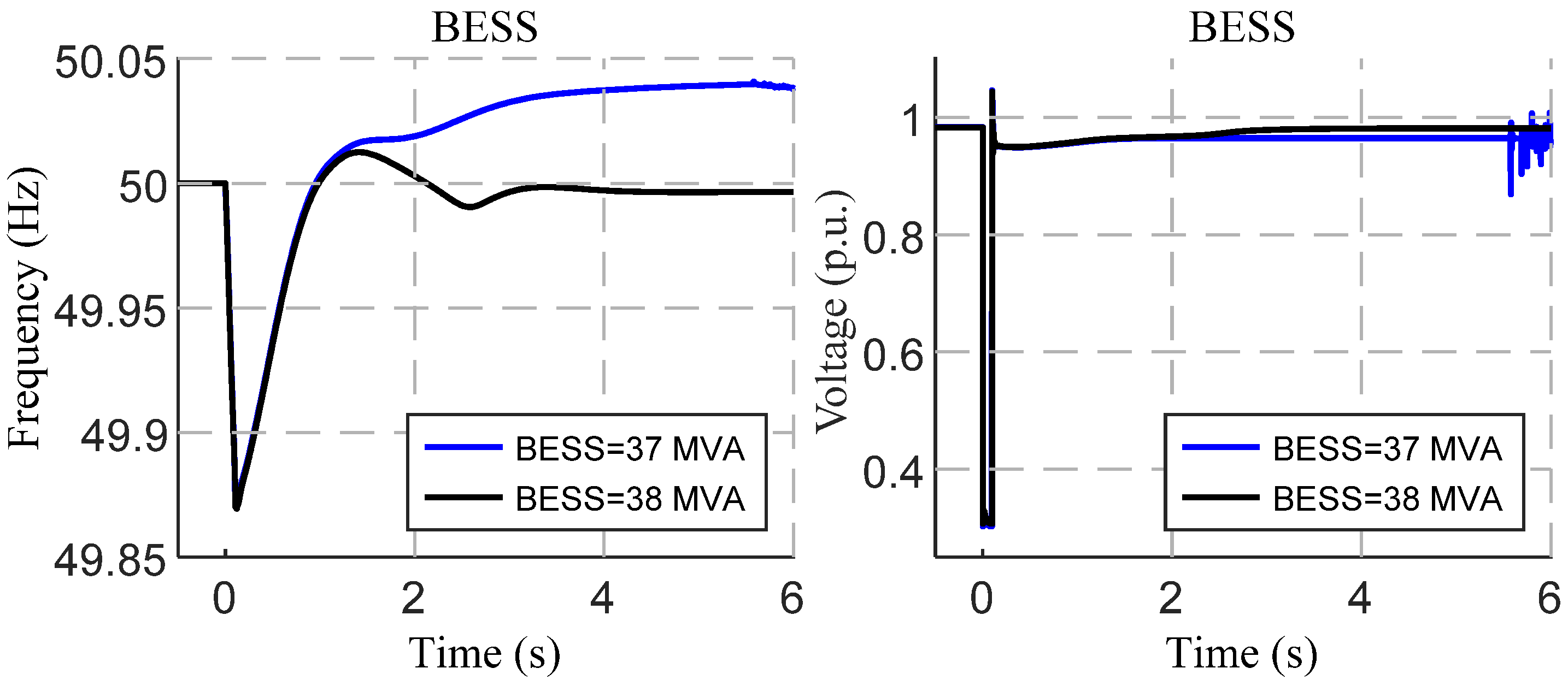
Taking into account the load distribution presented in Table 2, it is intended to determine the minimum required BESS power converter capacity that ensures the post-fault recovery of all IM loads. As can be observed in Figure 9, for a BESS power converter sizing lower than 38 MVA, the small industrial motor connected to L3 stalls following the fault clearance. This is due to the large reactive power consumption required by the IM after the network fault clearance, which demands a large reactive power from the BESS power converter for about 2–3 s after the voltage recovery, as it can be observed in Figure 10. Furthermore, in Figure 11, the network frequency and voltage measured at bus B1 are depicted, with the large voltage oscillations for the 37 MVA BESS power converter case being notable, which is a consequence of the L3 small industrial motor stall. In both cases, a similar network frequency drop induced by the short circuit is observed. From this analysis, it is concluded that the initial BESS power converter sizing is not suitable when considering dynamic load modeling (it is intended for the post-fault recovery of all IM loads).
4.2.2. Induction Motor Inertia—Sensitivity Analysis
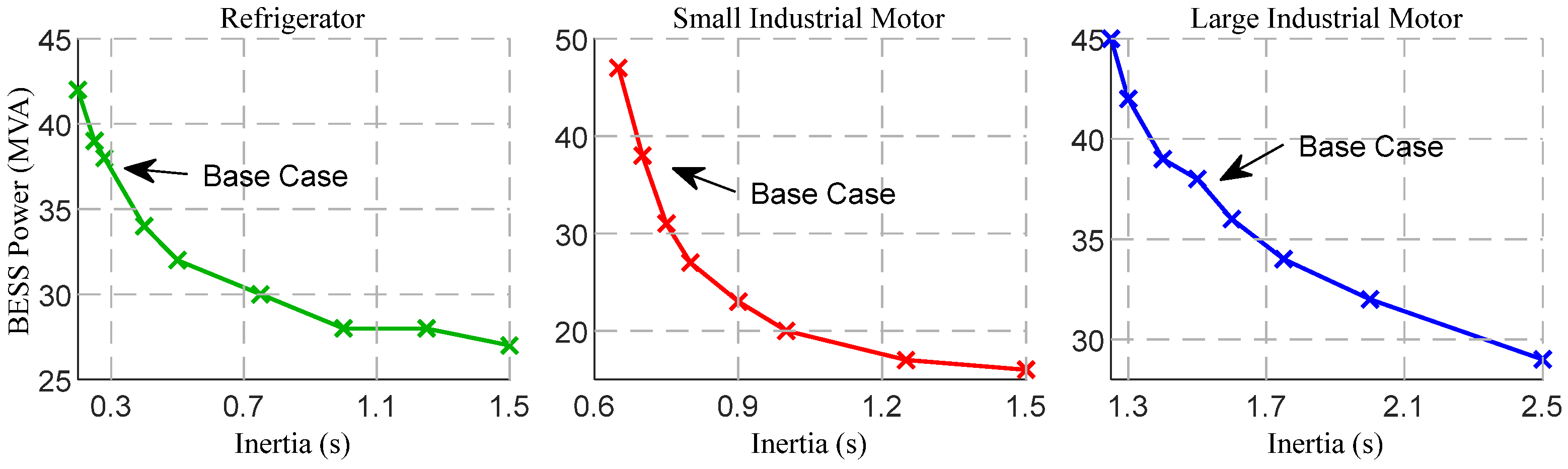
The influence of IM inertia on the grid-forming BESS power converter sizing is analyzed in this subsection. The default inertia constant of each IM type is available in Table A1 (in Appendix A). In Figure 12, the correspondent results are shown, where for each inertia value, the correspondent required minimum BESS power converter sizing for assuring the successful recovery of all IM loads following fault clearance is presented. Note that three independent sensitivity analyses were performed for each IM class. In each analysis, only the inertia constant of one IM class was modified (e.g., for the IM refrigerator type analysis—green line in Figure 12—the inertia constant of the refrigerator-type IM was varied within the range presented on the x-axis, while the inertia constants of the small and large industrial motor types remained at the corresponding default values—Table A1). It was concluded that increasing the IM inertia is beneficial since it allows reducing the BESS converter power sizing. This is due to the fact that higher IM inertia contributes to lower IM speed variations and hence lower recovery currents following fault clearance.
4.2.3. Induction Motor Load Percentage—Sensitivity Analysis
In this subsection, it is intended to evaluate the influence of the IM load percentage on the BESS power converter sizing. Note that in the base case scenario (Section 4.2.1), 26.5% of IM load was considered. The results are presented in Table 3 (for the cases where L3 and/or L5 were not modeled as IM loads, their modeling is based on a constant impedance). A general trend to reduce the BESS power converter capacity with the reduction in the IM load ratio is verified. In fact, higher shares of IM loads will require larger reactive current consumption during the post-fault period, which in turn will induce a larger reactive current injection from the BESS power converter. However, the IM load location also presents some influence on the BESS power converter sizing. For instance, for the case where the IM load is only modeled by L1, the required BESS capacity is smaller than the base case, which presents a lower IM load ratio.
In addition, the short-circuit critical clearing time (CCT) for different shares of IM load integration was analyzed, considering a 12 MVA BESS power converter sizing (suitable for system operation while considering static load modeling—Section 4.1). As can be observed in Table 4, there is a clear trend for the CCT reduction as a function of the IM load ratio reduction. Note that for the case where L2 is modeled as an IM load, a 12 MVA BESS power converter is not enough to guarantee the IM load recovery after a fault occurrence, independently of its duration.
4.2.4. Fault Duration—Sensitivity Analysis
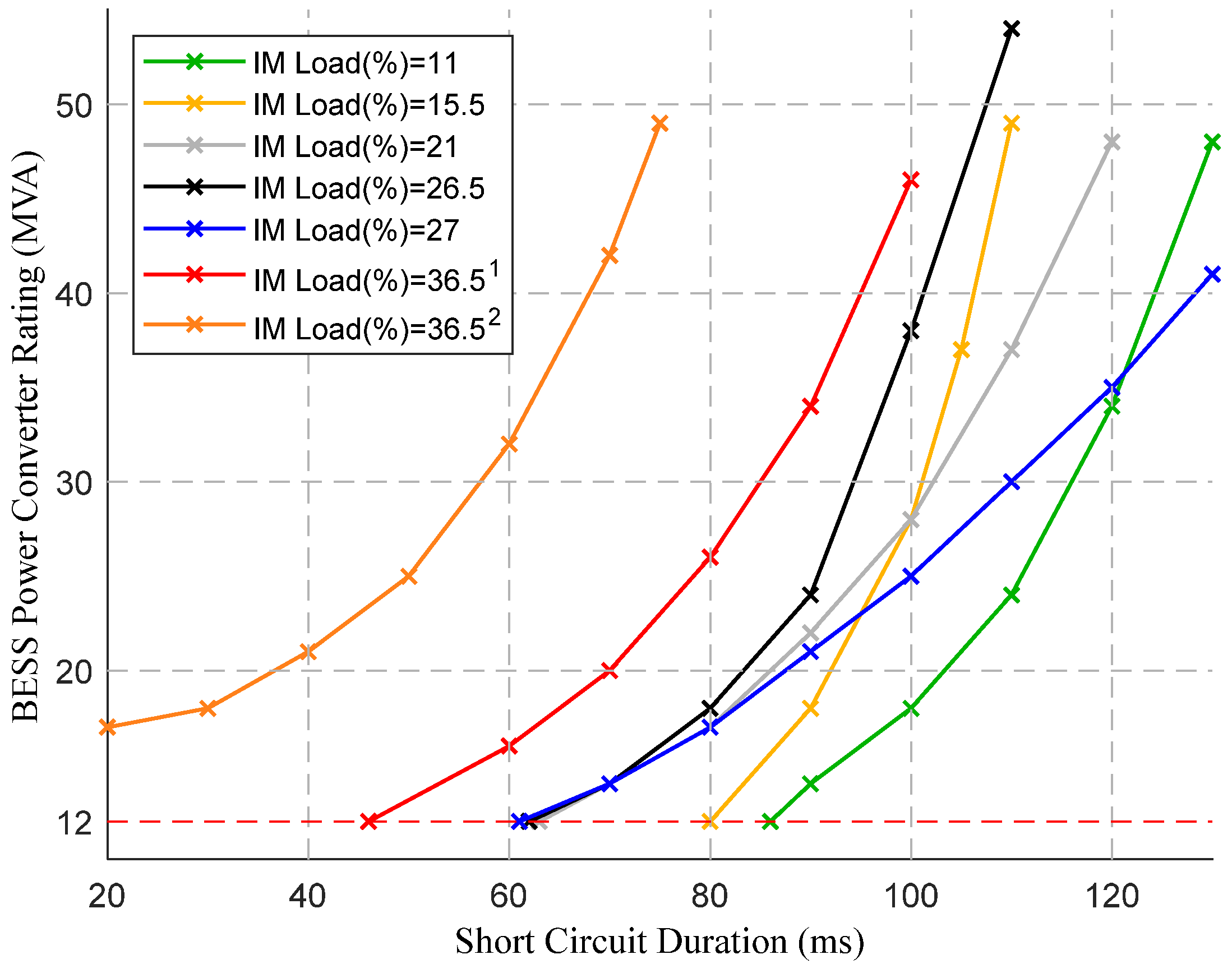
This analysis intends to address the influence of the network fault duration on the BESS power sizing. In this sense, a sensitivity analysis is presented in Figure 13, showing the minimum required BESS power converter capacity for distinct short-circuit times. Note that all the different IM load percentage scenarios presented in Table 3 were considered (“” corresponds to “L3 + L4 + L5”, while “” corresponds to “L2”). As expected, the longer short circuits require a higher BESS power capacity.
4.2.5. Induction Motor Composition—Sensitivity Analysis
Lastly, the influence of the IM load composition on the required BESS power converter capacity is analyzed. Therefore, in Figure 14, the results of the performed analysis are shown, matching each IM load composition scenario with the respective minimum BESS power converter capacity (the refrigerator and small and large industrial IM loads are represented as Ref, SIM and LIM, respectively). As it can be observed, different IM load compositions lead to different BESS power converter sizing requirements. Thus, it is noticeable that both the small and, in particular, the large industrial IM load types require a larger BESS power converter capacity compared with the refrigerator motor type.
5. Control Strategies for the Mitigation of the Impacts Induced by Induction Motor Loads
The results presented in Section 4 highlight that large shares of IM loads are responsible for an increased post-fault reactive current contribution from the BESS power converter required for the re-excitation of the IM loads (which can be observed in Figure 9). An immediate solution for this problem may consist in increasing the sizing of the BESS power converter, as it was also illustrated in the previous section. Nevertheless, alternative solutions based on the exploitation of advanced control strategies for the available power electronic interfaces are proposed in order to minimize the impacts that IM loads may bring, during the post-fault recovery period, with respect to BESS power converter oversizing.
An alternative and simple solution to mitigate this issue consists of adopting undervoltage IM load shedding mechanisms [33]. However, in this work, it is intended to propose solutions which ensure the complete recovery of all the network IM loads while profiting from the control flexibility available in all the power electronic interfaces. Therefore, two distinct approaches are proposed. The first approach consists of implementing appropriated control solutions at the CI-RES, aiming to increase their ability to provide a post-fault reactive current to re-excite the IM loads and hence support the grid (this control solution is presented in Section 5.1). Complementarily, the second approach consists of a dynamic modulation of the reference voltage of the grid-forming unit during the post-fault period, aiming to increase the post-fault electromagnetic torque in IM loads and hence contribute to its reacceleration (this solution is presented in Section 5.2). In order to evaluate the effectiveness of the proposed solutions, the operational scenario presented in Section 4.2.1 is considered, where the BESS power converter capacity is assumed to be 12 MVA. A 100 ms three-phase symmetrical short circuit reference incidente occurring at t = 0 s of the simulation time in the transmission line interconnecting buses and (see Figure 6) is considered. Finally, in Section 5.3, it is demonstrated that the coordinated implementation of these two control solutions is beneficial in operating scenarios with very large shares of IM loads.
5.1. Fault Ride Through Strategy for Grid-Following Units
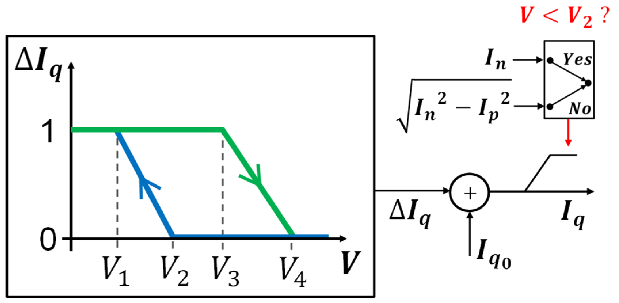
Recently, insular network operators developed new grid codes which provide specific FRT capabilities to the grid-following CI-RES, namely, involving voltage-sensitive active and/or reactive current injections [34,35]. However, in this paper, it is demonstrated that these voltage/current requirements should be adapted in order to facilitate the accommodation of 100% CI-RES generation penetration levels in networks with high shares of IM loads. Hence, a novel voltage/reactive current strategy for the grid-following CI-RES is proposed. From Figure 11 (base case), it is verified that after the fault clearance, the network voltage returns almost instantaneously to a value close to its nominal value. However, from Figure 9 and Figure 10, a large reactive power injection from the BESS power converter is observed for about 2–3 s after the voltage recovery, which is due to the IM reactive power consumption in the moments subsequent to the fault clearance. This post-fault behavior evidences the need for large amounts of reactive power support in the moments subsequent to the fault clearance. In the proposed solution, CI-RES interfaces are intended to contribute to the provision of the reactive current in the reacceleration phase of IM loads.
Aiming to better exploit the available resources in this period, the proposed control strategy consists of a voltage/reactive current hysteresis-type characteristic, instead of the well-known voltage/reactive current droop control, as depicted in Figure 15. As it can be observed in the proposed solution, for voltage dips lower than , the reactive current injection will be defined by the blue curve, injecting 1 p.u. of reactive current when the CI-RES terminal voltage reaches This trajectory depicted in blue corresponds to the CI-RES terminal voltage decrease following a network fault. When the CI-RES terminal voltage increases and reaches , the voltage/reactive current characteristic switches to the green curve, returning to the blue curve when the CI-RES terminal voltage reaches . The use of this hysteresis-type voltage/reactive current injection curve might lead to situations in which the post-fault reactive power injection is different from the pre-fault one. Such situation can be easily overpassed by a manual intervention of the system operator to reset the reactive power setpoint of the units or by a local reset action at the CI-RES interface a few seconds following post-fault voltage stabilization. It is also important to notice that for CI-RES terminal voltage values lower than , priority will be given to the reactive current injection; otherwise, priority will be given to the active current injection. The goal of prioritizing the active current injection for is intended to improve the system stability when the voltage reaches values closer to the nominal one, where active power consumption will also increase. However, this prolonged reactive current injection in the correspondent period () will only be achieved for cases where the CI-RES is not operated at its maximum active power capacity before fault occurrence, being limited as a function of the active current setpoint () and of the converter nominal current (). Therefore, for these operational scenarios, exploiting the solution in the BESS power converter is also necessary to facilitate IM load recovery.
5.1.1. Simulation Results and Discussion
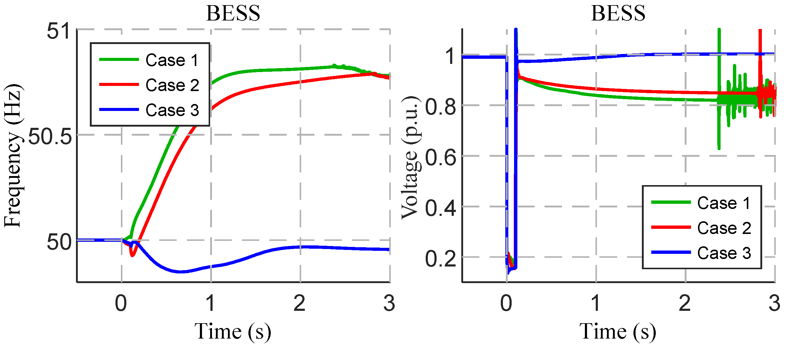
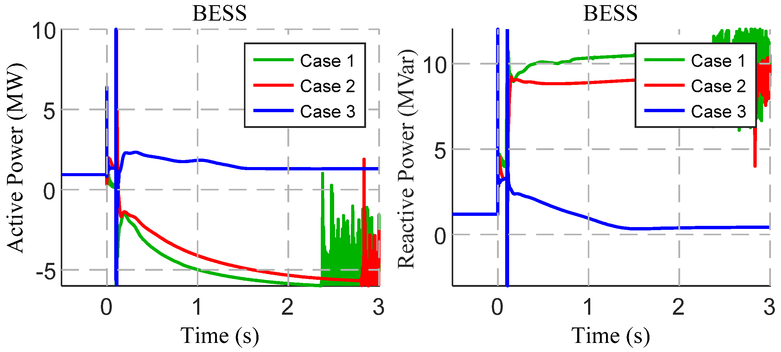
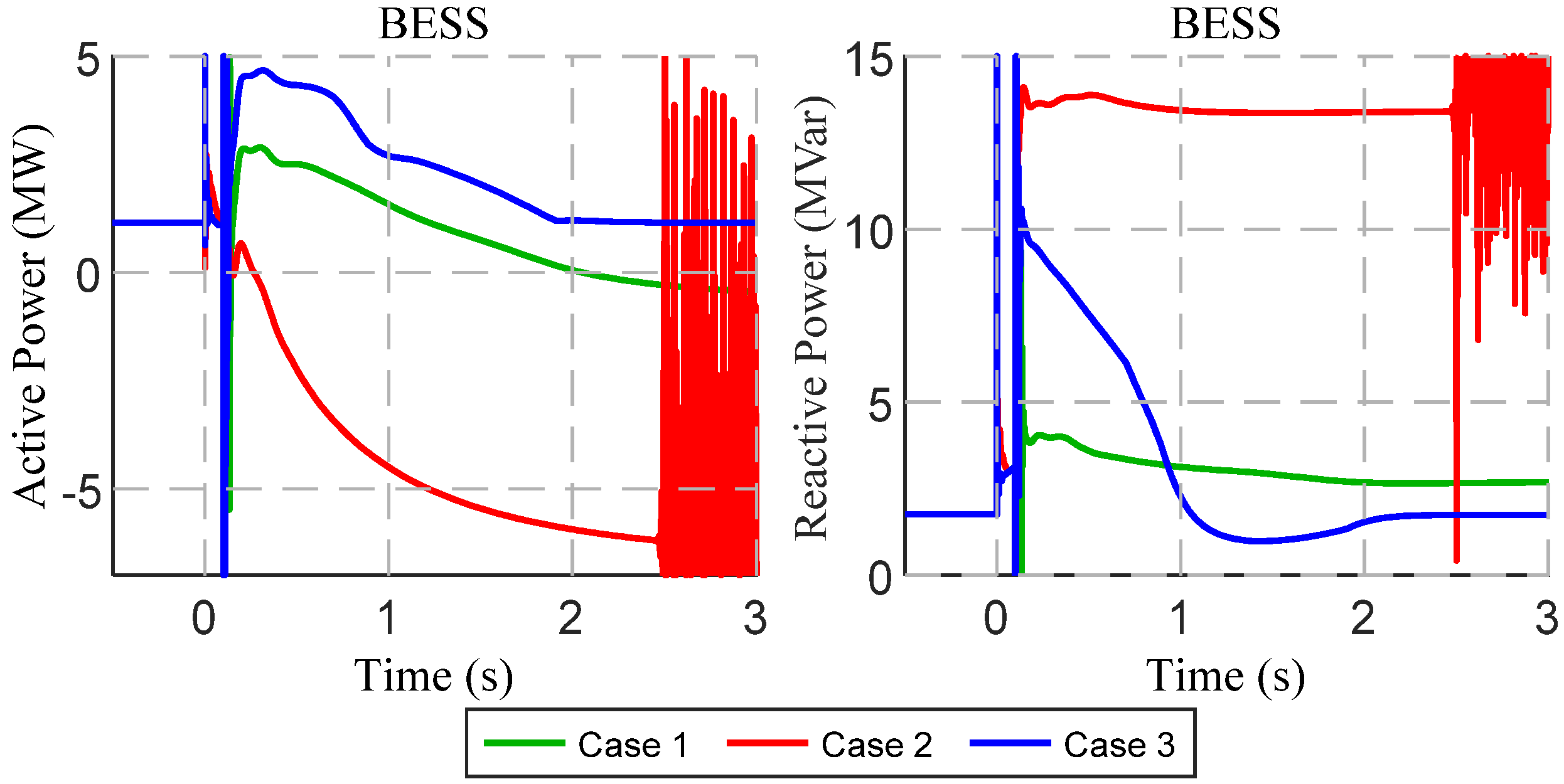
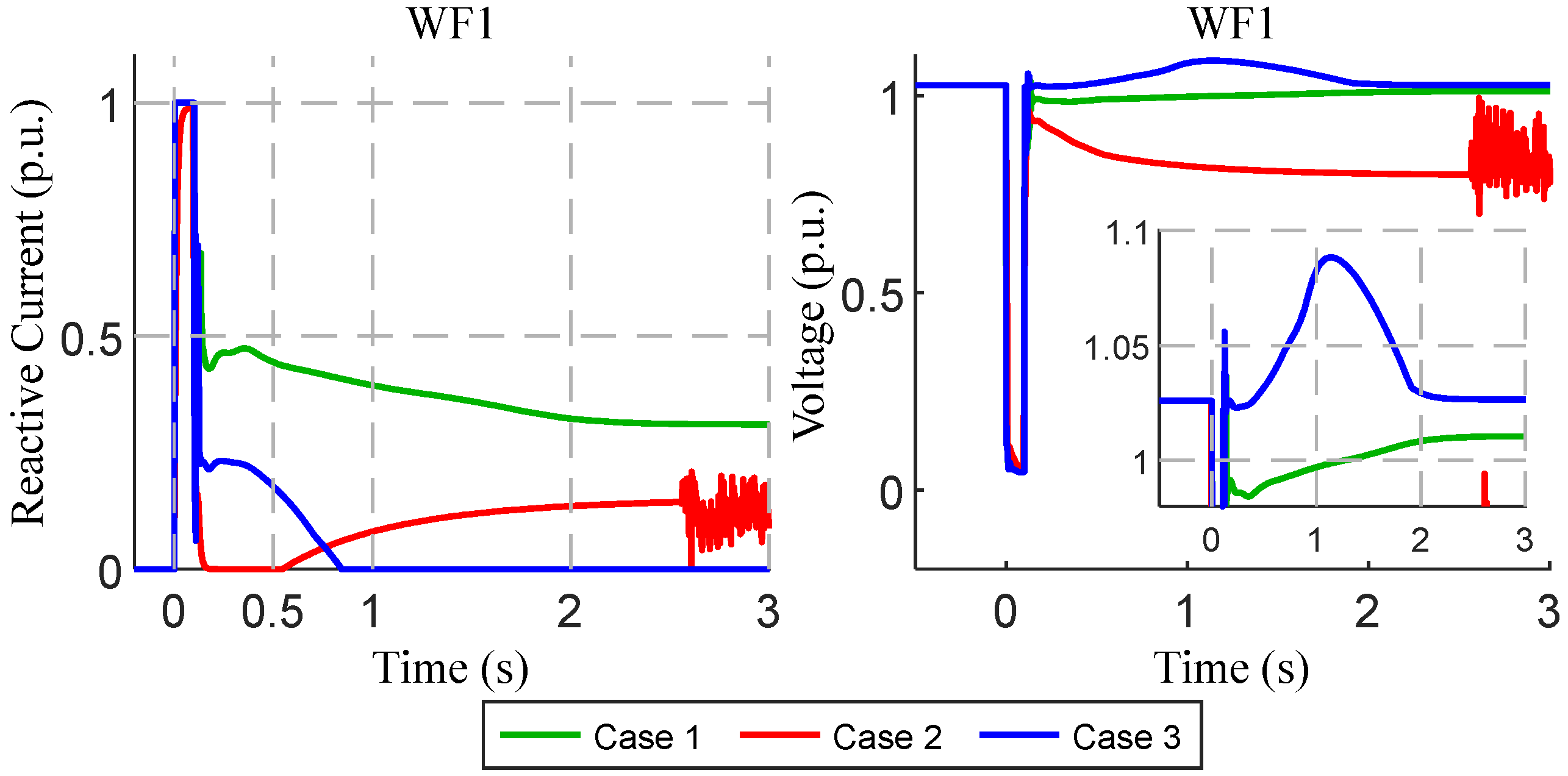
In order to demonstrate the performance of the proposed control solution with respect to the ability to provide improved conditions for post-fault IM load reacceleration, three distinct conditions are compared in this subsection: (Case 1) Voltage/active and reactive current dynamic control imposed by the system operator of Madeira Island [26], [34]. In this case, priority is given to the active current injection during the short-circuit event, whose contribution should be, at least, equal to the pre-fault active current injection. Simultaneously, the reactive current should be injected proportionally to the terminal voltage of the generation unit (a voltage dead-band of 0.1 p.u. and a voltage/reactive current control gain equal to −2.5 were considered). (Case 2) Voltage/reactive current dynamic control, similar to the requirement imposed by the Spanish insular grid code [35,36]. In this case, priority is given to the reactive current injection, being proportional to the terminal voltage of the generation unit (a voltage dead-band of 0.1 p.u. and a voltage/reactive current control gain equal to −2.5 were considered). (Case 3) The voltage/reactive current strategy presented in Figure 15, where = 0.5 p.u., = 0.9 p.u., = 0.9 p.u. and = 1.06 p.u.
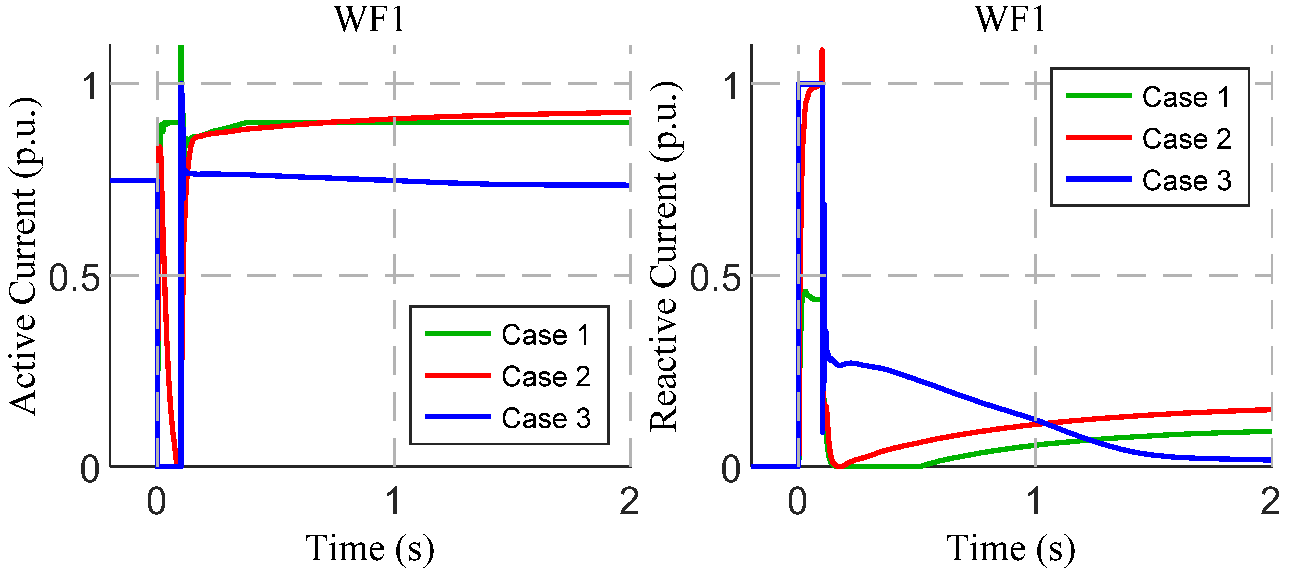
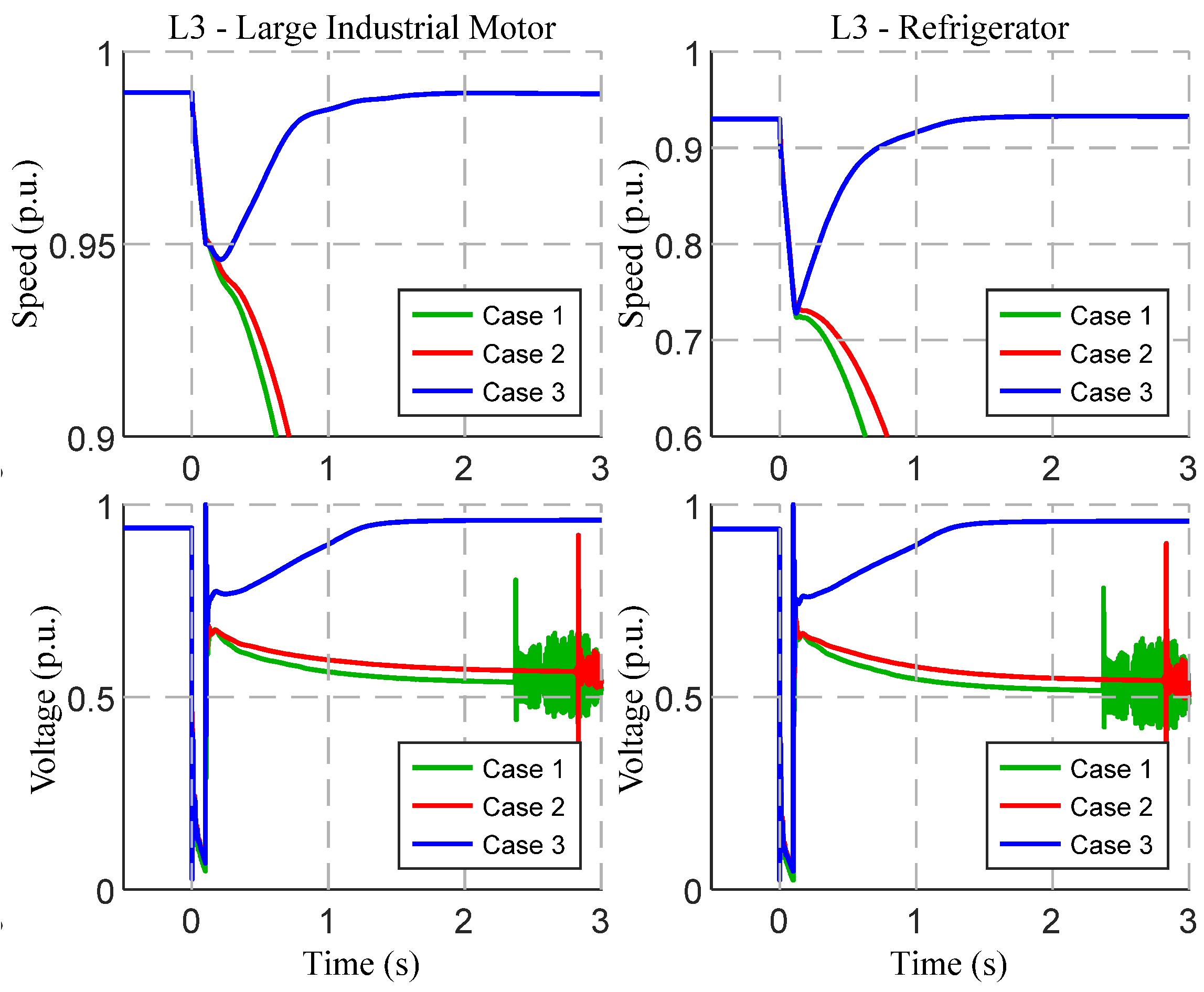
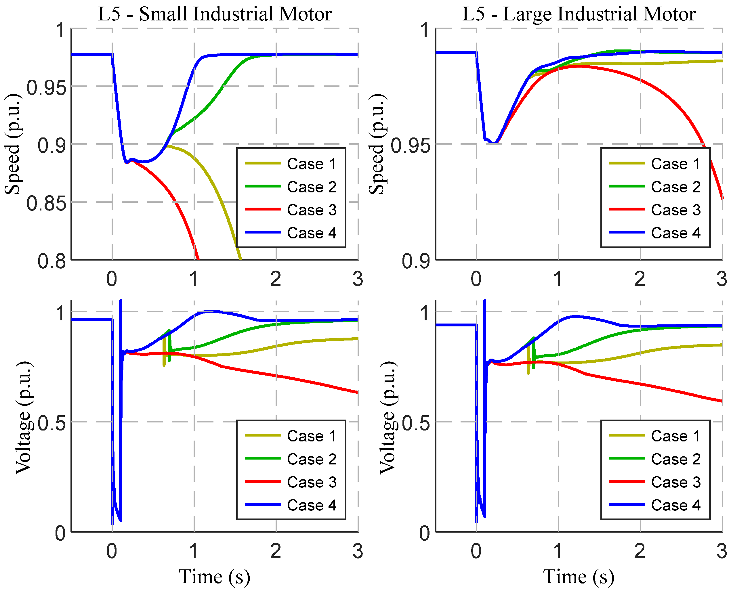
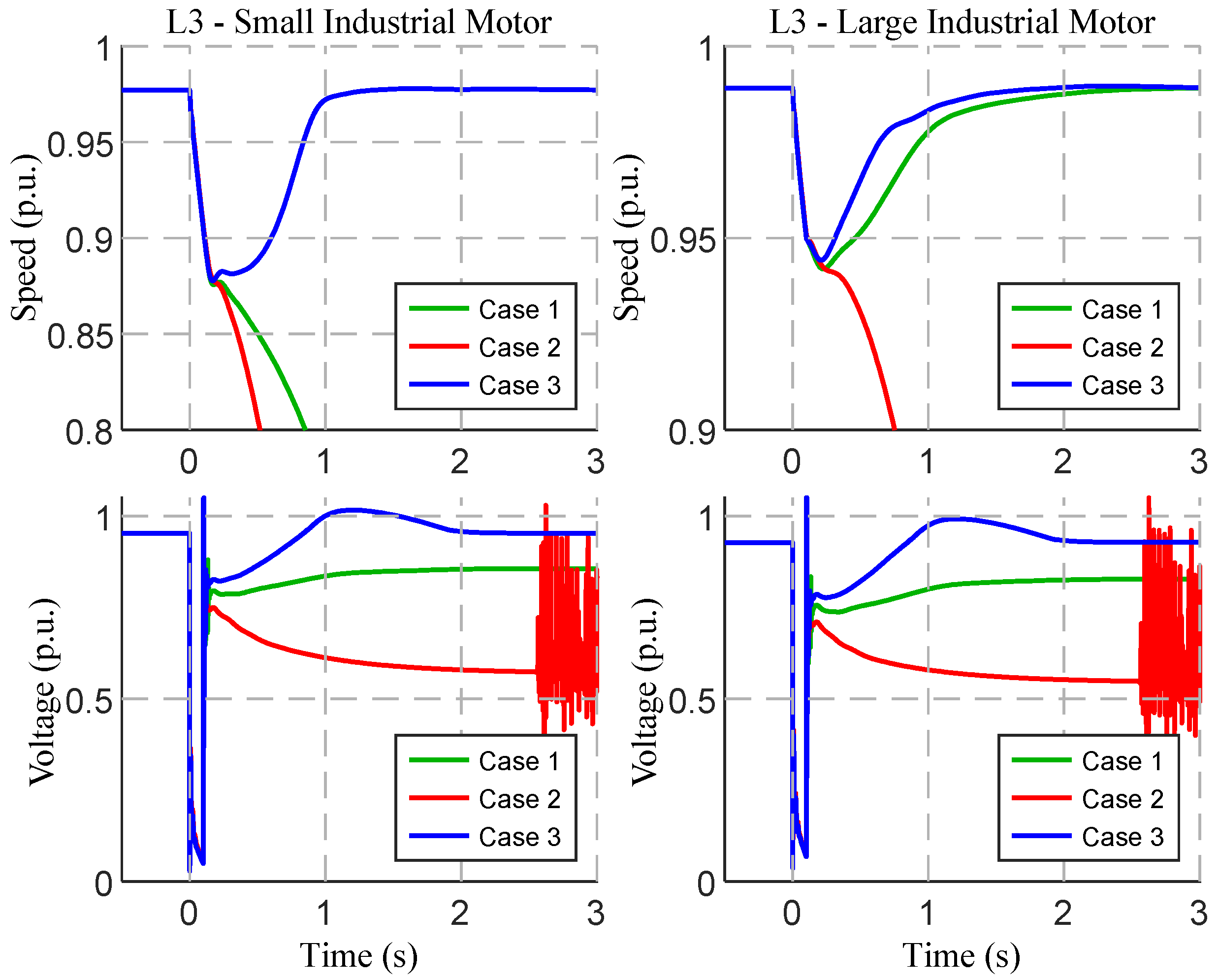
As it can be observed in Figure 16, only in Case 3, where the proposed strategy is adopted, is it possible to assure a successful recovery of all IM loads and hence the stabilization of the grid frequency and network voltage when the 12 MVA BESS power converter capacity is assumed. In addition, the control strategy employed in Case 3 successfully reduces the BESS reactive power contribution following the fault clearance compared to the other cases, as it can be observed from the results presented in Figure 17 (note that the use of the hysteresis-type solution led to a reactive current injection stabilization different from the pre-fault state). It is also observed that the BESS pre-fault active power regime is achieved approximately 1.5 s after the fault clearance. In Figure 18, the CI-RES active and reactive current outputs (only the WF1 response is presented since all CI-RES generators present a similar dynamic behavior) are depicted, being notable that, only in Case 3, a relevant post-fault reactive current injection after the fault clearance is observed, which is a result of the proposed voltage/reactive current hysteresis-type characteristic. Finally, from Figure 19, it is evidenced that the IM load (L3 is presented as an illustrative example) only recovers after the network short-circuit clearance in Case 3. It is also demonstrated that the prolonged CI-RES reactive current injection contributes to increase the IM load terminal voltage in the moments subsequent to the fault clearance, due to a faster re-excitation, thus contributing to a faster IM load reacceleration.
In conclusion, the obtained results demonstrate that the complete recovery of all IM loads is only accomplished in Case 3. This is due to the contribution provided by the prolonged reactive current injection from the CI-RES to the grid (as can be observed in Figure 18), which is not observed for Cases 1 and 2. Thus, in Cases 1 and 2, without the prolonged contribution of the CI-RES, the BESS power converter is not able to provide the necessary reactive current amount required for the successful re-excitation of the IM loads following the fault clearance.
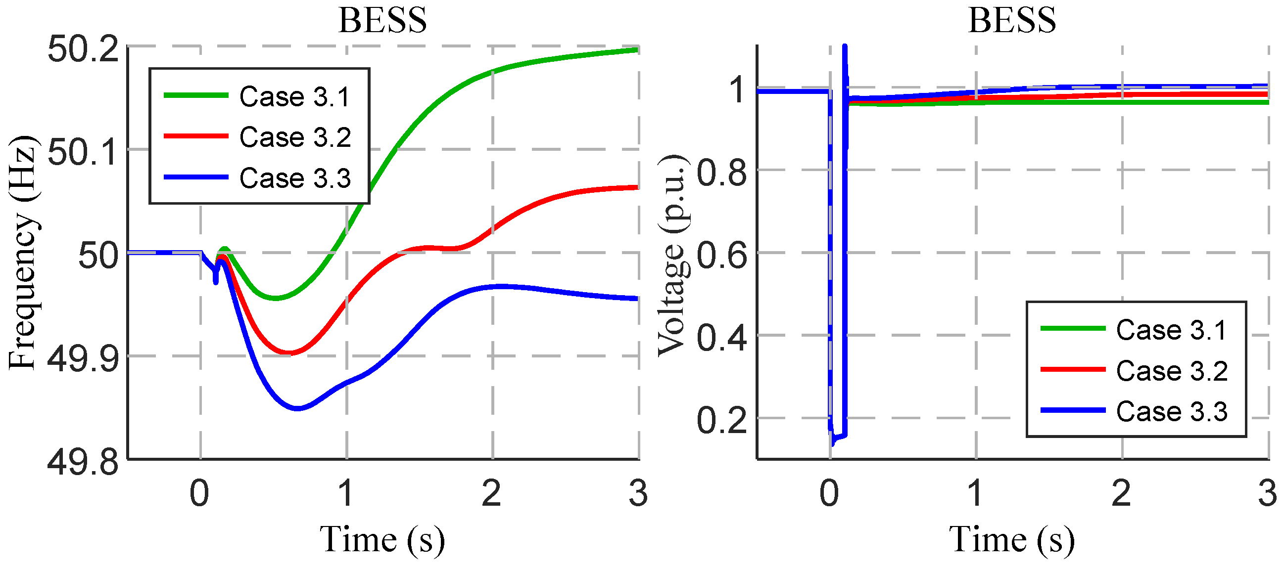
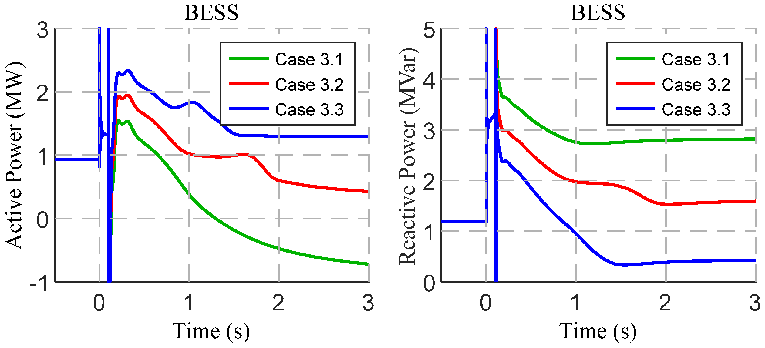
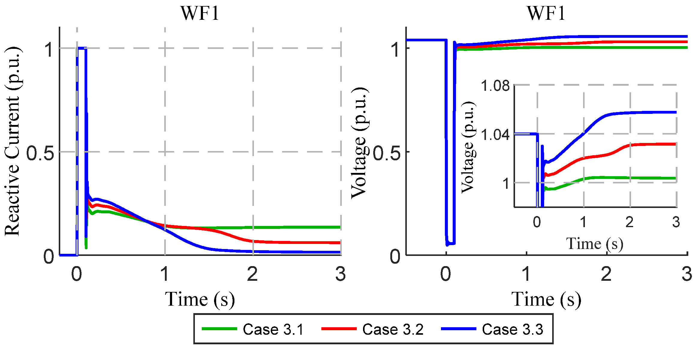
Aiming to provide a better understanding regarding the influence of the proposed voltage/reactive current hysteresis tuning, a sensitivity analysis was also performed. In this sense, three distinct sets of parameters were compared: (Case 3.1) = 0.5 p.u., = 0.9 p.u., = 0.9 p.u. and = 1.02 p.u.; (Case 3.2) = 0.5 p.u., = 0.9 p.u., = 0.9 p.u. and = 1.04 p.u.; (Case 3.3) = 0.5 p.u., = 0.9 p.u., = 0.9 p.u. and = 1.06 p.u.
The corresponding results are depicted in Figure 20, Figure 21, Figure 22 and Figure 23. From the conducted analysis, it was verified that successful IM load recovery occurs only in Case 3.2 and Case 3.3, indicating that the CI-RES reactive current contribution in Case 3.1 is not sufficient. Furthermore, it was observed that higher values of allow an increased reactive current injection by the CI-RES during the post-fault period (Figure 22), revealing the less reactive power regulation effort by the BESS power converter (Figure 21) and a faster voltage recovery at the IM load terminals (Figure 23). From Figure 22, it is also notable that lower values of lead to a higher reactive power injection from the BESS power converter. On the other hand, it is noticeable that higher values of cause a post-fault steady-state network voltage increase. Therefore, should not be too high, in order to prevent overvoltages. Moreover, as the adopted control parameters influence the post-fault voltage, the loads’ active power consumption is also affected because of the adopted load model. Consequently, slight variations in the network frequency are observed as a result of this sensitivity analysis (Figure 20).
5.1.2. Robustness Analysis
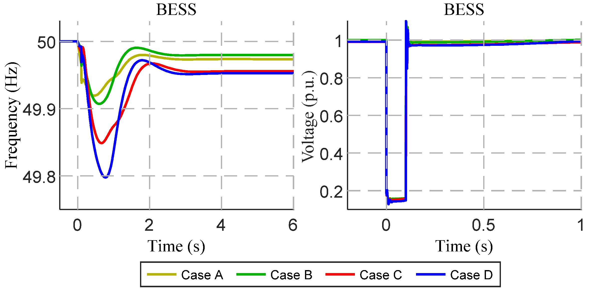
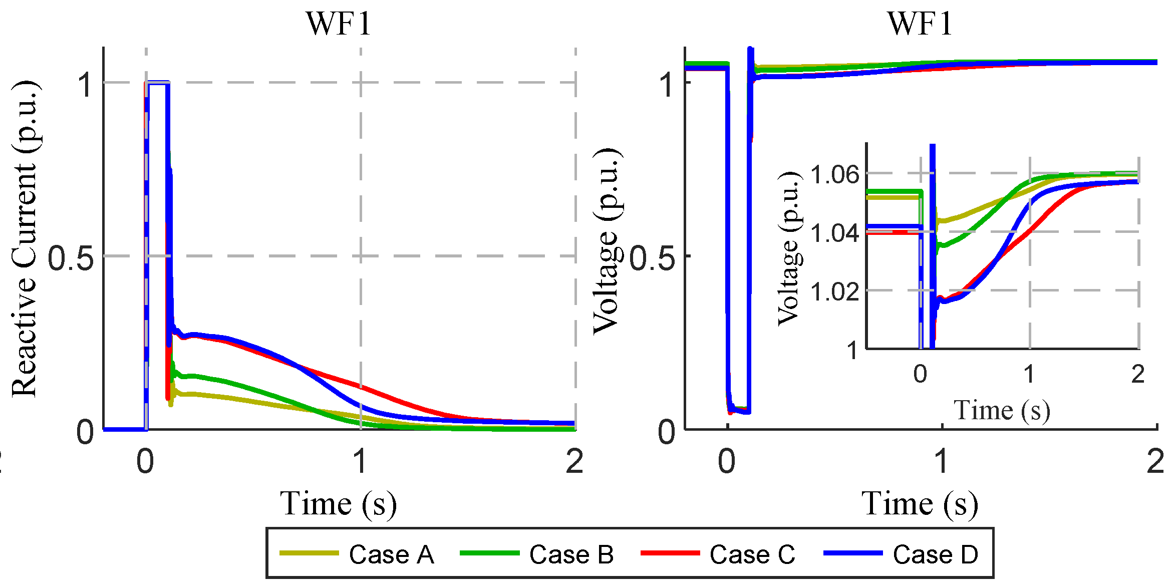
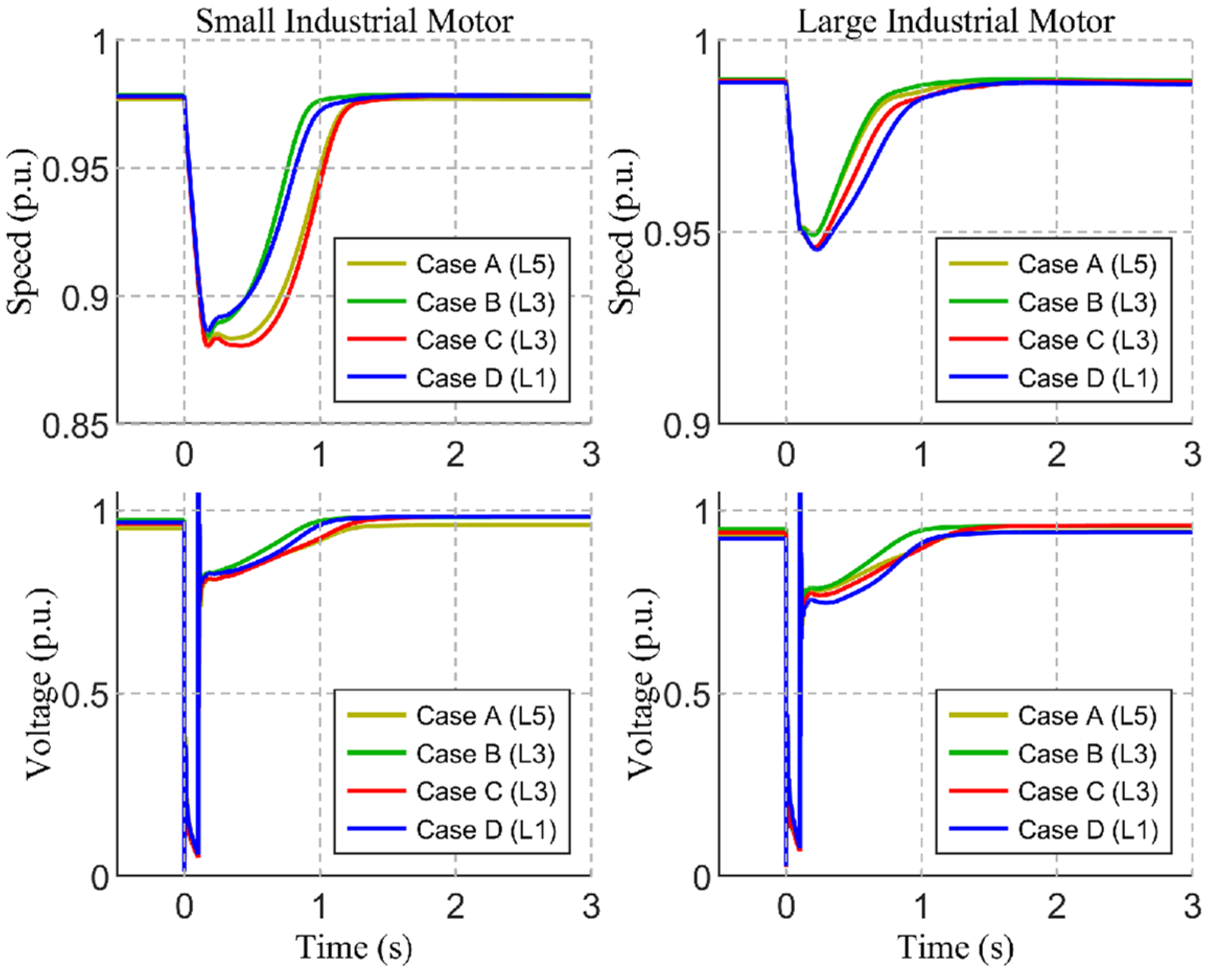
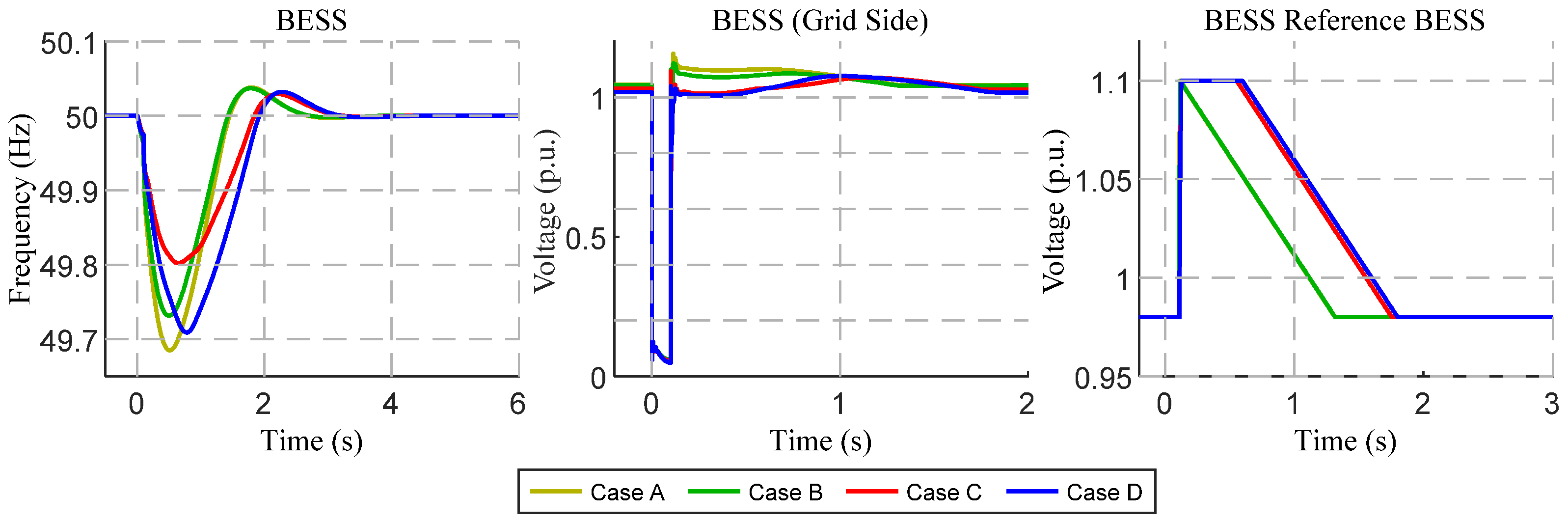
The purpose of the analysis performed in this subsection is to validate the robustness of the proposed CI-RES FRT strategy (presented in Figure 15) and the control tuning proposed in Case 3 (= 0.5 p.u., = 0.9 p.u. and = 1.06 p.u.). Thus, the corresponding solution was tested in several conditions contemplating different percentages of the IM load while considering the same operational scenario (Table 1). In this sense, four distinct cases were compared regarding the IM load percentage: (Case A) 11% of IM load ( load); (Case B) 15.5% of IM load ( load); (Case C) 26.5% of IM load (+ load); (Case D) 27% of IM load ( load).
The obtained results are depicted in Figure 24, Figure 25 and Figure 26. In the test cases with high shares of IM loads (Cases C and D), an increased reactive current contribution by the CI-RES during the post-fault period is verified, since more reactive power will be consumed by the IM loads, which decreases the network voltage profiles (as verified in Figure 25 and Figure 26). Nonetheless, the recovery of all the IM loads is ensured for all the test cases.
5.1.3. Contribution of the Proposed Strategy to BESS Power Converter Sizing
Aiming to demonstrate the benefits of the proposed CI-RES FRT strategy, the sensitivity analysis performed in Section 4.2.3 was revisited (considering the FRT control strategy presented in Figure 15 implemented in the existing SPP and WF—see Figure 6). From Table 5, it is demonstrated that the BESS power converter sizing is significantly reduced when the proposed post-fault reactive current recovery is considered, compared with the results previously presented in Table 3. As can be observed, only the cases with an IM load percentage of 36.5% require a BESS power converter larger than the initial sizing (12 MVA). In addition, the short-circuit CCT (considering a 12 MVA BESS power converter) was also recalculated, which is presented in Table 6. From the obtained results, it is possible to conclude that the CCT increased significantly when compared with the results presented in Table 4.
5.2. VSM Voltage Magnitude Control Strategy
From the results obtained in Section 5.1, it was concluded that the prolonged reactive current injection provided by the CI-RES during the post-fault period contributes to increasing the network voltage profiles (as shown in Figure 19), which increases the IM loads’ electromagnetic torque and contributes to a successful reacceleration. In this section, an alternative control solution which exploits the VSM post-fault reference voltage modulation is presented, which can be temporarily increased in order to boost the reacceleration torque developed by IM loads. Note that in this section, the CI-RES FRT strategy corresponds to the one presented in Section 2.2.
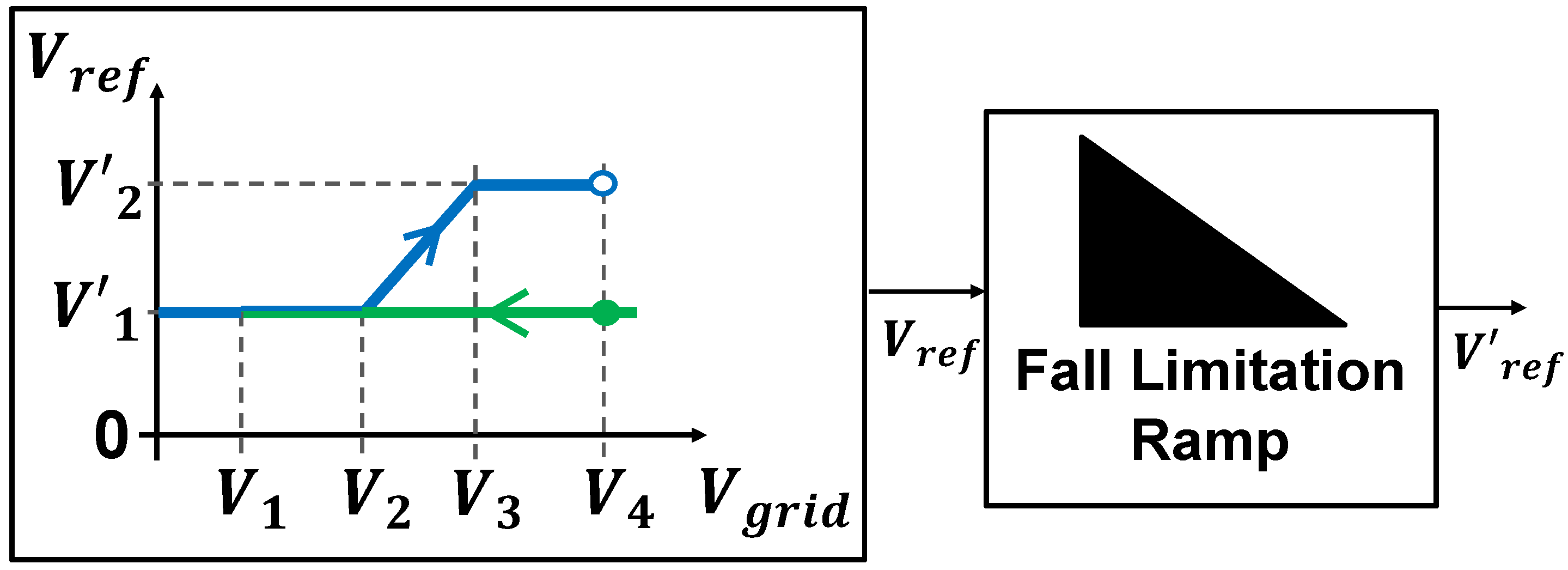
As explained in Section 2.1.3, the VSM output voltage amplitude is defined as a function of the voltage reference (constant value) and of a reactive power/voltage modulation term. However, in order to temporarily increase the VSM reference voltage during the post-fault recovery period, a hysteresis control approach is considered, modulating the VSM reference voltage as a function of the VSM terminal voltage (at the grid side), as shown in Figure 27. Thus, during steady-state operation will be defined by the green curve, being fixed at . However, for voltage dips lower than , the VSM reference voltage will be defined by the blue curve, returning to the green curve when the VSM terminal voltage reaches . In order to smooth the transition from the blue curve to the green curve, a fall limitation ramp is imposed on the VSM reference voltage.
5.2.1. Simulation Results and Discussion
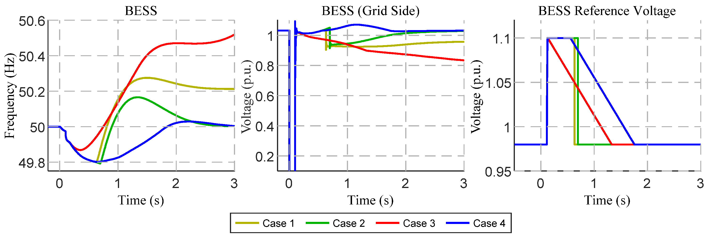
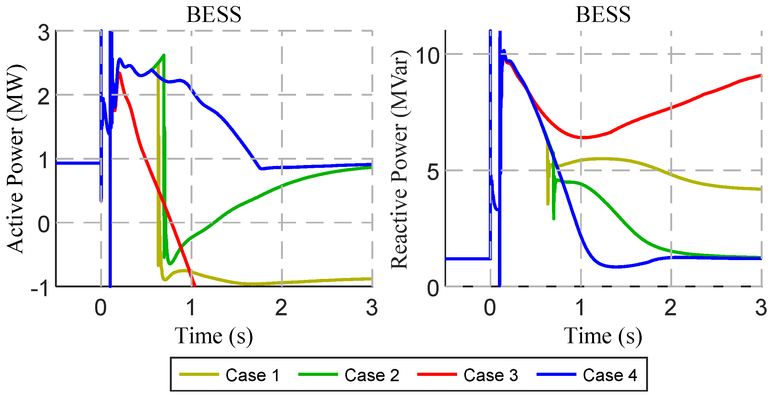
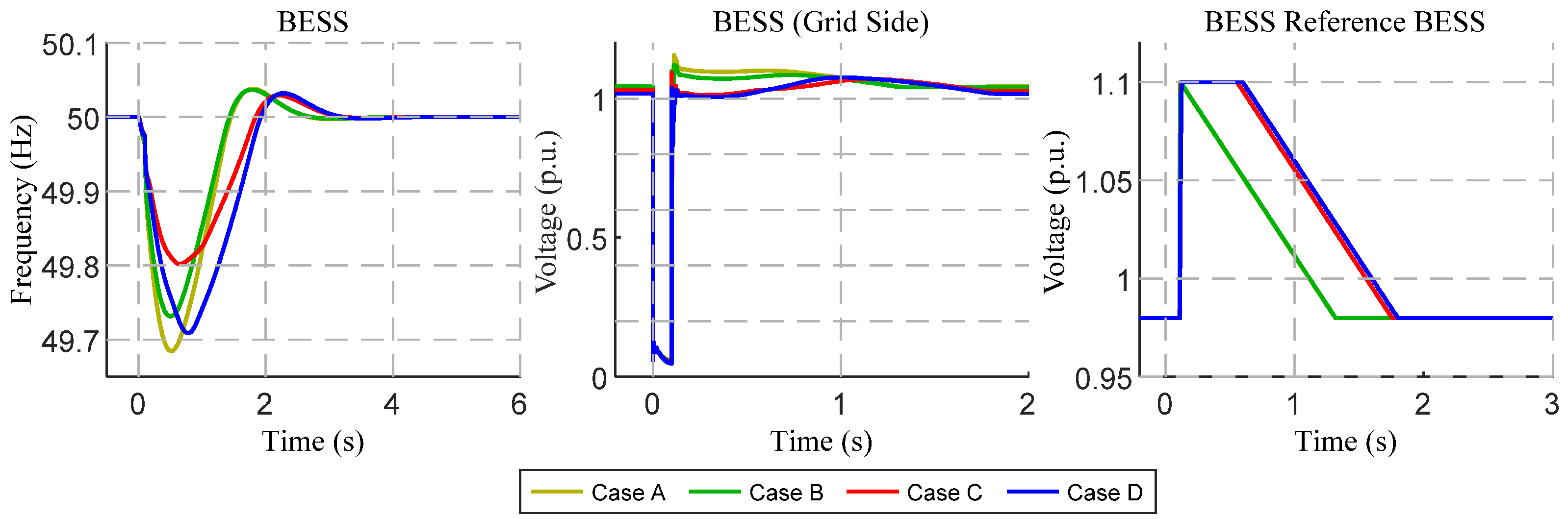
In order to demonstrate the effectiveness of the proposed solution and to provide a better understanding regarding the VSM reference voltage/terminal voltage hysteresis tunning, a sensitivity analysis was performed. Three distinct sets of parameters were compared, where = 0.5 p.u., = 0.8 p.u., = 1 p.u., = 0.98 p.u. and = 1.1 p.u. constitute a common parametrization in all test cases: (Case 1) = 1.04 p.u. and a limitation ramp of −999 p.u. (V)/s (it was considered a step transition from the blue curve to the green curve); (Case 2) = 1.05 p.u. and a limitation ramp of −999 p.u. (V)/s; (Case 3) = 1.02 p.u. and a limitation ramp of −0.1 p.u. (V)/s; (Case 4) = 1.03 p.u. and a limitation ramp of −0.1 p.u. (V)/s.
The obtained results are presented in Figure 28, Figure 29 and Figure 30. As can be observed, the IM load recovery is only accomplished in Case 2 and Case 4. Furthermore, it was observed that the fall limitation ramp ensures a smooth transition between the hysteresis’s blue curve and green curve. Therefore, in Case 4, it is verified that the BESS pre-fault frequency and voltage regime is achieved approximately 2 s after the fault clearance.
5.2.2. Robustness Analysis
A robustness analysis is presented, similar to the analysis performed in Section 5.1.2, aiming to validate the proposed BESS power converter voltage control strategy (presented in Figure 27) and the control tuning proposed in Case 3 (= 0.5 p.u., = 0.8 p.u., = 1 p.u., = 1.03 p.u., = 0.98 p.u., = 1.1 p.u. and a limitation ramp of −0.1 p.u. (V)/s). Thus, the corresponding solution was tested in the following four distinct cases: (Case A) 11% of IM load ( load); (Case B) 15.5% of IM load ( load); (Case C) 26.5% of IM load ( + load); Case D) 27% of IM load ( load). The results are presented in Figure 31 and Figure 32. As can be observed, the recovery of all the IM loads is ensured for all the test cases.
5.2.3. Contribution of the Proposed Strategy to BESS Power Converter Sizing
In order to show the benefits of the proposed strategy and respective parametrization (see Section 5.2.2), the sensitivity analysis performed in Section 4.2.3 was revisited. A side-by-side comparison between the sensitivity analysis of Section 4.2.3 (case base), of Section 5.1.3 (strategy 1) and of the voltage magnitude control strategy proposed in Figure 27 (strategy 2) is presented.
The results of strategy 1 and strategy 2 are similar, being demonstrated in Table 7 that the BESS power converter sizing is significantly reduced when strategy 1 or strategy 2 is considered, in comparison with the results of the base case. As can be observed, only the cases with an IM load percentage of 36.5% require a BESS power converter larger than 12 MVA. In addition, the short-circuit CCT, considering a 12 MVA BESS power converter, is presented in Table 8. Similarly, it is concluded that strategy 1 and strategy 2 are able to significantly increase the CCT compared to the base case.
5.3. Conbined Use of the Proposed Control Strategies
In Section 5.1 and Section 5.2, two distinct solutions were presented, which have proven to, individually, be effective with respect to the provision of improved reacceleration of IM loads following a network fault. However, as previously mentioned, the results of Section 5.1 and Section 5.2 were obtained considering the operational scenario presented in Section 4.2.1 (which comprises 26.5% of IM loads).
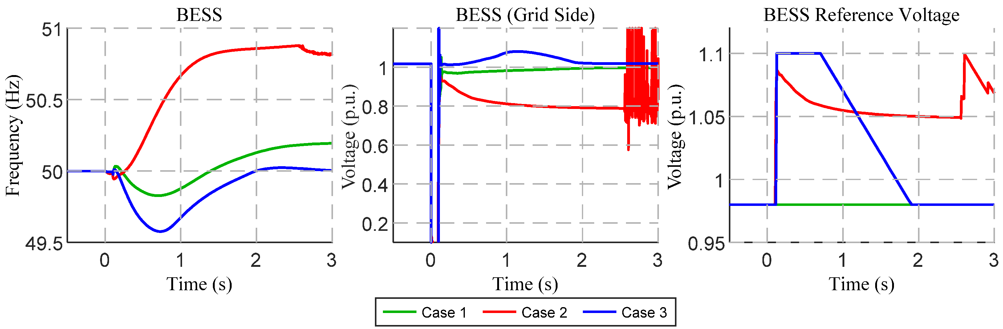
Hence, in extreme operating conditions with large shares of IM loads, it may be interesting to simultaneously implement and adopt the two considered solutions. For this purpose, in this section, the same operational scenario was considered (Table 1); however, this time, 42.5% of IM load was integrated ( and were modeled as IM loads—see Table 2). Thus, three distinct test cases were compared: (Case 1) the FRT strategy presented in Figure 15 was implemented in the grid-following units, where = 0.5 p.u., = 0.9 p.u., = 0.9 p.u. and = 1.06 p.u. (same parametrization as Section 5.1.2), with the VSM reference voltage being fixed to = 0.98 p.u.; (Case 2) the implemented FRT strategy in the grid-following units corresponds to the strategy presented in Section 2.2, where the voltage magnitude control strategy presented in Figure 27 was implemented in the BESS ( = 0.5 p.u., = 0.8 p.u., = 1 p.u., = 1.03 p.u., = 0.98 p.u., = 1.1 p.u. and a limitation ramp of −0.1 p.u. (V)/s—same parametrization as Section 5.2.2); (Case 3) both proposed strategies were considered, using the parametrization of Case 1 and Case 2.
The results are presented in Figure 33, Figure 34, Figure 35 and Figure 36, with it being observed that only in Case 3 is the full recovery of all IM loads assured. Moreover, it is also verified that the BESS pre-fault frequency and voltage regime is achieved approximately 2 s after the fault clearance. In Figure 35, it is observed that the combination of the two presented control strategies induced a post-fault voltage increase, within the admissible range, that positively contributed to the reacceleration of all the IM loads.
In summary, the results demonstrate that the individual contributions of the proposed control solutions presented in Section 5.1 (Case 1) and Section 5.2 (Case 2) were not capable of ensuring the re-excitation of the IM loads in operational scenarios with very large shares of IM loads (despite being effective in operational scenarios with moderate shares of IM loads). In this sense, it was concluded that by combining the control effort provided by the two control strategies, it was possible to successfully re-excite all the IM loads in the moments subsequent to the fault clearance.
6. Conclusions
This paper focused on isolated power systems operating exclusively with converter-based generation, in which a BESS, whose power converter is controlled as a grid-forming unit, is responsible for providing network regulation capabilities. Within that scope, it was intended to analyze the impact of load dynamics on the BESS power converter sizing. For the case in which the network load is modeled only by static models, a BESS power converter capacity complying with the N-1 security criterion is enough to ensure the network dynamic stability. However, converter-interfaced BESSs have a very limited overcurrent capability, which constitutes a major disadvantage when dynamic loads are connected to the grid. Thus, it was also concluded that the presence of IM loads leads to negative effects on the network dynamics following large voltage disturbances due to their large reactive power consumption in the moments subsequent to a fault clearance. In this sense, it is necessary to oversize the BESS power converter capacity in order to cope with short-circuit events, aiming to assure IM load recovery in contrast to undervoltage shedding. An extensive sensitivity analysis was performed, providing a clear understanding of how the load model, composition and parametrization affect the oversizing of the BESS power converter capacity.
Furthermore, it was demonstrated that the FRT requirements currently demanded by the insular grid codes need to be revised in order to facilitate the operating scenarios with 100% penetration levels of converter-based generation in isolated networks with a significative percentage of the IM load composition. For this purpose, a novel FRT control mode was identified and discussed for the CI-RES. The proposed FRT mode is intended to increase the reactive current contribution of these units in the moments subsequent to the fault clearance, which corresponds to the moments where IM loads demand higher reactive currents for recovering their operation. In addition, it was demonstrated that the dynamic modulation of the reference voltage of the grid-forming unit during the post-fault period contributes to a faster re-magnetization of IM loads, which consequently increases their electromagnetic torque, hence contributing to its reacceleration. Therefore, it is concluded that a proper network load characterization by the respective network operators, as well as the adoption of appropriate advanced control functionalities at the power electronic interfaces existing in the converter-based generators, should avoid BESS power converter oversizing for specific applications in isolated systems.
Author Contributions
Preparation of the manuscript was performed by J.G., C.L.M. and J.A.P.L. All authors have read and agreed to the published version of the manuscript.
Funding
This research was funded by ERDF—European Regional Development Fund through the Operational Programme for Competitiveness and Internationalisation—COMPETE 2020 Programme, and by National Funds through the Portuguese funding agency, FCT—Fundação para a Ciência e a Tecnologia, within project ESGRIDS.
Institutional Review Board Statement
Not applicable.
Informed Consent Statement
Not applicable.
Data Availability Statement
The data presented in this study are available on request from the corresponding author. The data are not publicly available due to privacy issues.
Conflicts of Interest
The authors declare no conflict of interest.
Appendix A

Table A1.
Motor load parametrization in p.u. [31].
Table A1.
Motor load parametrization in p.u. [31].
| Parameters | Refrigerator | Small Industrial Motor | Large Industrial Motor |
|---|---|---|---|
| Rs | 0.056 | 0.031 | 0.013 |
| Xs | 0.087 | 0.1 | 0.067 |
| Rr | 0.053 | 0.018 | 0.170 |
| Xr | 0.082 | 0.18 | 0.009 |
| Xm | 2.4 | 3.2 | 3.8 |
| H | 0.28 | 0.7 | 1.5 |
Table A2.
Grid-forming default control parameters.
| Parameter | Units | Value |
|---|---|---|
| Nominal Voltage | V | 400 |
| Filter Resistance | p.u. | 0.01 |
| Filter Inductance | p.u. | 0.1 |
| Inertia Constant () | s | 5 |
| Damping Constant () | p.u. | 10 |
| Q-V Droop Gain () | p.u. | 0.1 |
| P-f Droop Gain () | p.u. | 0.04 |
| P-f Integral Gain () | p.u. | 0 |
| TVI Resistance () | p.u. | 1.125 |
| TVI Reactance () | p.u. | 1.125 |
| TVI Current Threshold () | p.u. | 1.8 |
| TVI Maximum Current () | p.u. | 2 |
References
- Mayhorn, E.; Xie, L.; Butler-Purry, K.L. Multi-time Scale Coordination of Distributed Energy Resources in Isolated Power Systems. IEEE Trans. Smart Grid 2016, 8, 998–1005. [Google Scholar] [CrossRef]
- Psarros, G.N.; Karamanou, E.G.; Papathanassiou, S.A. Feasibility Analysis of Centralized Storage Facilities in Isolated Grids. IEEE Trans. Sustain. Energy 2018, 9, 1822–1832. [Google Scholar] [CrossRef]
- Kroposki, B.; Johnson, B.; Zhang, Y.; Gevorgian, V.; Denholm, P.; Hodge, B.M.; Hannegan, B. Achieving a 100% Renewable Grid: Operating Electric Power Systems with Extremely High Levels of Variable Re-newable Energy. IEEE Power Energy Mag. 2017, 15, 61–73. [Google Scholar] [CrossRef]
- Matevosyan, J.; Vital, V.; O’Sullivan, J.; Quint, R.; Badrzadeh, B.; Prevost, T.; Quitmann, E.; Ramasubramanian, D.; Urdal, H.; Achilles, S.; et al. Grid-Forming Inverters: Are They the Key for High Renewable Penetration? IEEE Power Energy Mag. 2019, 17, 89–98. [Google Scholar] [CrossRef]
- D’Arco, S.; Suul, J.A. Equivalence of Virtual Synchronous Machines and Frequency-Droops for Converter-Based Mi-croGrids. IEEE Trans. Smart Grid 2014, 5, 394–395. [Google Scholar] [CrossRef]
- Mo, O.; D’Arco, S.; Suul, J.A. Evaluation of Virtual Synchronous Machines with Dynamic or Quasi-Stationary Machine Models. IEEE Trans. Ind. Electron. 2017, 64, 5952–5962. [Google Scholar] [CrossRef] [Green Version]
- Zhong, Q.-C.; Weiss, G. Synchronverters: Inverters That Mimic Synchronous Generators. IEEE Trans. Ind. Electron. 2011, 58, 1259–1267. [Google Scholar] [CrossRef]
- Zhang, W.; Remon, D.; Rodríguez, D.R. Frequency support characteristics of grid-interactive power converters based on the synchronous power controller. IET Renew. Power Gener. 2017, 11, 470–479. [Google Scholar] [CrossRef] [Green Version]
- Milanovic, J.V.; Yamashita, K.; Villanueva, S.M.; Djokic, S.Ž.; Korunović, L.M. International Industry Practice on Power System Load Modeling. IEEE Trans. Power Syst. 2013, 28, 3038–3046. [Google Scholar] [CrossRef]
- Mishra, Y.; Hill, D.; Ma, J.; Dong, Z. Induction motor load impact on power system eigenvalue sensitivity analysis. IET Gener. Transm. Distrib. 2009, 3, 690–700. [Google Scholar] [CrossRef]
- Wang, C.; Wang, Z.; Wang, J.; Zhao, D. Load Modeling—A Review. IEEE Trans. Smart Grid 2018, 9, 5986–5999. [Google Scholar]
- Renmu, H.; Jin, M.; Hill, D. Composite Load Modeling via Measurement Approach. IEEE Trans. Power Syst. 2006, 21, 663–672. [Google Scholar] [CrossRef]
- Chang, G.W.; Chen, C.I.; Liu, Y.J. A Neural-Network-Based Method of Modeling Electric Arc Furnace Load for Power Engi-neering Study. IEEE Trans. Power Syst. 2010, 25, 138–146. [Google Scholar] [CrossRef]
- Shao, S.; Pipattanasomporn, M.; Rahman, S. Development of physical-based demand response-enabled residential load models. IEEE Trans. Power Syst. 2013, 28, 607–614. [Google Scholar] [CrossRef]
- Fulgêncio, N.; Moreira, C.; Carvalho, L.; Lopes, J.P. Aggregated dynamic model of active distribution networks for large voltage disturbances. Electr. Power Syst. Res. 2020, 178, 106006. [Google Scholar] [CrossRef]
- Tuffner, F.K.; Schneider, K.P.; Hansen, J.; Elizondo, M.A. Modeling Load Dynamics to Support Resiliency-Based Opera-tions in Low-Inertia Microgrids. IEEE Trans. Smart Grid 2019, 10, 2726–2737. [Google Scholar] [CrossRef]
- Diaz, G.; Gonzalez-Moran, C.; Gomez-Aleixandre, J.; Diez, A. Composite Loads in Stand-Alone Inverter-Based Mi-crogrids—Modeling Procedure and Effects on Load Margin. IEEE Trans. Power Syst. 2010, 25, 894–905. [Google Scholar] [CrossRef]
- Chen, J.; Chen, J. Stability Analysis and Parameters Optimization of Islanded Microgrid with Both Ideal and Dynamic Constant Power Loads. IEEE Trans. Ind. Electron. 2018, 65, 3263–3274. [Google Scholar] [CrossRef]
- Kahrobaeian, A.; Mohamed, Y.A.R.I. Analysis and Mitigation of Low-Frequency Instabilities in Autonomous Medi-um-Voltage Converter-Based Microgrids with Dynamic Loads. IEEE Trans. Ind. Electron. 2014, 61, 1643–1658. [Google Scholar] [CrossRef]
- Penaloza, J.D.R.; Adu, J.A.; Borghetti, A.; Napolitano, F.; Tossani, F.; Nucci, C.A. Influence of load dynamic response on the stability of microgrids during islanding transition. Electr. Power Syst. Res. 2021, 190, 106607. [Google Scholar] [CrossRef]
- Rouhani, A.; Abur, A. Real-Time Dynamic Parameter Estimation for an Exponential Dynamic Load Model. IEEE Trans. Smart Grid 2016, 7, 1530–1536. [Google Scholar] [CrossRef]
- North American Electric Reliability Corporation (NERC). A Technical Reference Paper Fault-Induced Delayed Voltage Re-covery. Transmission Issues Subcommittee and System Protection and Control Subcommittee. June 2019. Available online: http://www.nerc.com/docs/pc/tis/FIDVR_Tech_Ref%20V1-2_PC_Approved.pdf (accessed on 5 March 2021).
- Mercier, P.; Cherkaoui, R.; Oudalov, A. Optimizing a Battery Energy Storage System for Frequency Control Application in an Isolated Power System. IEEE Trans. Power Syst. 2009, 24, 1469–1477. [Google Scholar] [CrossRef]
- Markovic, U.; Haberle, V.; Shchetinin, D.; Hug, G.; Callaway, D.; Vrettos, E. Optimal Sizing and Tuning of Storage Capacity for Fast Frequency Control in Low-Inertia Systems. In Proceedings of the 2019 International Conference on Smart Energy Systems and Technologies (SEST), Porto, Portugal, 9–11 September 2019; IEEE: New York, NY, USA, 2019; pp. 1–6. [Google Scholar]
- O’Sullivan, J.; Rogers, A.; Flynn, D.; Smith, P.; Mullane, A.; O’Malley, M. Studying the Maximum Instantaneous Non-Synchronous Generation in an Island System—Frequency Stability Challenges in Ireland. IEEE Trans. Power Syst. 2014, 29, 2943–2951. [Google Scholar] [CrossRef] [Green Version]
- Beires, P.P.; Moreira, C.L.; Lopes, J.P.; Figueira, A.G. Defining connection requirements for autonomous power systems. IET Renew. Power Gener. 2020, 14, 3–12. [Google Scholar] [CrossRef]
- Lopes, J.A.P.; Moreira, C.L.; Madureira, A.G. Defining Control Strategies for MicroGrids Islanded Operation. IEEE Trans. Power Syst. 2006, 21, 916–924. [Google Scholar] [CrossRef] [Green Version]
- Gkountaras, A. Modeling Techniques and Control Strategies for Inverter Dominated Microgrids. Ph.D. Thesis, Universitätsverlag der TU Berlin, Berlin, Germany, 2016. [Google Scholar]
- Denis, G.; Prevost, T.; DeBry, M.; Xavier, F.; Guillaud, X.; Menze, A. The Migrate project: The challenges of operating a transmission grid with only inverter-based generation. A grid-forming control improvement with transient current-limiting control. IET Renew. Power Gener. 2018, 12, 523–529. [Google Scholar] [CrossRef]
- Beires, P.; Vasconcelos, M.H.; Moreira, C.L.; Lopes, J.P. Stability of autonomous power systems with reversible hydro power plants. Electr. Power Syst. Res. 2018, 158, 1–14. [Google Scholar] [CrossRef]
- Taylor, C.W. Power System Voltage Stability; Maratukulam, D. Power System Voltage Stability; Maratukulam, D., Balu, N.J., Eds.; Palo Alto: Santa Clara, CA, USA, 1994. [Google Scholar]
- Gouveia, J.; Moreira, C.L.; Lopes, J.P. Grid-Forming Inverters Sizing in Islanded Power Systems—A stability per-spective. In Proceedings of the 2019 International Conference on Smart Energy Systems and Technologies (SEST), Porto, Portugal, 9–11 September 2019; pp. 1–6. [Google Scholar]
- Otomega, B.; Glavic, M.; Van Cutsem, T. Distributed Undervoltage Load Shedding. IEEE Trans. Power Syst. 2007, 22, 2283–2284. [Google Scholar] [CrossRef] [Green Version]
- Madeira Island Grid Code. Decreto Regulamentar Regional nº 8/2019/M, Região Autónoma da Madeira. 2019. Available online: https://dre.pt/application/conteudo/125865392 (accessed on 5 March 2021).
- Spanish Insular Grid Code. Red Eléctrica de España, P.O. 12.2. 2018. Available online: https://www.boe.es/eli/es/res/2018/02/01/(3) (accessed on 5 March 2021).
- Rodrigues, E.; Osório, G.; Godina, R.; Bizuayehu, A.; Lujano-Rojas, J.; Catalão, J.P.S. Grid code reinforcements for deeper renewable generation in insular energy systems. Renew. Sustain. Energy Rev. 2016, 53, 163–177. [Google Scholar] [CrossRef]
Figure 1.
Schematic view of the battery energy storage system (BESS) converter control.

Figure 2.
Virtual synchronous machine control loop.

Figure 3.
Reactive power–voltage control loop.

Figure 4.
Transient virtual impedance loop.

Figure 5.
Converter-interfaced renewable energy source power control model (adapted from [30]).
Figure 5.
Converter-interfaced renewable energy source power control model (adapted from [30]).

Figure 6.
Single-line diagram of the studied isolated power system.

Figure 7.
BESS power converter synthetic frequency and terminal voltage: exponential load model active power coefficient sensitivity analysis.
Figure 7.
BESS power converter synthetic frequency and terminal voltage: exponential load model active power coefficient sensitivity analysis.

Figure 8.
BESS power converter synthetic frequency and terminal voltage: exponential load model reactive power coefficient sensitivity analysis.
Figure 8.
BESS power converter synthetic frequency and terminal voltage: exponential load model reactive power coefficient sensitivity analysis.

Figure 9.
L3 small industrial motor speed and reactive power consumption—base case scenario.

Figure 10.
BESS power converter active and reactive power outputs—base case scenario.

Figure 11.
BESS power converter synthetic frequency and terminal voltage—base case scenario.

Figure 12.
BESS power converter rating vs. induction motor (IM) load inertia sensitivity analysis with respect to different motor load types.
Figure 12.
BESS power converter rating vs. induction motor (IM) load inertia sensitivity analysis with respect to different motor load types.

Figure 13.
BESS power converter sizing vs. fault duration as a function of the IM load percentage.

Figure 14.
Grid-forming BESS power converter sizing vs. IM load composition (Ref: refrigerator type; SIM: small industrial motor type; LIM: large industrial motor type).
Figure 14.
Grid-forming BESS power converter sizing vs. IM load composition (Ref: refrigerator type; SIM: small industrial motor type; LIM: large industrial motor type).

Figure 15.
Proposed reactive current/voltage strategy for converter-based generators operating as grid-following units.
Figure 15.
Proposed reactive current/voltage strategy for converter-based generators operating as grid-following units.

Figure 16.
BESS power converter synthetic frequency and terminal voltage for different reactive current-voltage injection profiles.
Figure 16.
BESS power converter synthetic frequency and terminal voltage for different reactive current-voltage injection profiles.

Figure 17.
BESS power converter active and reactive power outputs for different reactive current-voltage injection profiles.
Figure 17.
BESS power converter active and reactive power outputs for different reactive current-voltage injection profiles.

Figure 18.
WF1 active and reactive current outputs following different reactive current-voltage injection profiles.
Figure 18.
WF1 active and reactive current outputs following different reactive current-voltage injection profiles.

Figure 19.
L3 large industrial motor (left) and refrigerator load type motor (right) speeds and terminal voltages for different reactive current-voltage injection profiles adopted in CI-RES.
Figure 19.
L3 large industrial motor (left) and refrigerator load type motor (right) speeds and terminal voltages for different reactive current-voltage injection profiles adopted in CI-RES.

Figure 20.
BESS power converter synthetic frequency and terminal voltage regarding different shapes of the CI-RES voltage/reactive current hysteresis tuning.
Figure 20.
BESS power converter synthetic frequency and terminal voltage regarding different shapes of the CI-RES voltage/reactive current hysteresis tuning.

Figure 21.
BESS power converter active and reactive power outputs for different shapes of the CI-RES voltage/reactive current hysteresis tuning.
Figure 21.
BESS power converter active and reactive power outputs for different shapes of the CI-RES voltage/reactive current hysteresis tuning.

Figure 22.
WF1 reactive current output and terminal voltage following different voltage/reactive current hysteresis tuning.
Figure 22.
WF1 reactive current output and terminal voltage following different voltage/reactive current hysteresis tuning.

Figure 23.
L3 small and large industrial motors’ speeds and terminal voltages: influence resulting from voltage/reactive current hysteresis tuning.
Figure 23.
L3 small and large industrial motors’ speeds and terminal voltages: influence resulting from voltage/reactive current hysteresis tuning.

Figure 24.
BESS power converter synthetic frequency and terminal voltage with different IM load percentages.
Figure 24.
BESS power converter synthetic frequency and terminal voltage with different IM load percentages.

Figure 25.
WF1 reactive current output and terminal voltage considering different IM load percentages.
Figure 25.
WF1 reactive current output and terminal voltage considering different IM load percentages.

Figure 26.
Small and large industrial motors’ speeds and terminal voltages.

Figure 27.
Virtual synchronous machine reference voltage modulation.

Figure 28.
BESS power converter synthetic frequency, grid side terminal voltage and reference and voltage reference for voltage control loop.
Figure 28.
BESS power converter synthetic frequency, grid side terminal voltage and reference and voltage reference for voltage control loop.

Figure 29.
BESS power converter active and reactive power outputs.

Figure 30.
L3 large industrial motor (left) and refrigerator type motors (right) speeds and terminal voltages: influence resulting from different parametrizations of the VSM voltage reference generator.
Figure 30.
L3 large industrial motor (left) and refrigerator type motors (right) speeds and terminal voltages: influence resulting from different parametrizations of the VSM voltage reference generator.

Figure 31.
BESS power converter synthetic frequency and reference and terminal voltages: influence of different shares of IM loads.
Figure 31.
BESS power converter synthetic frequency and reference and terminal voltages: influence of different shares of IM loads.

Figure 32.
Small (left) and large (right) industrial motors’ speeds and terminal voltages.

Figure 33.
BESS power converter synthetic frequency, grid terminal voltage and reference and voltage reference for voltage control loop.
Figure 33.
BESS power converter synthetic frequency, grid terminal voltage and reference and voltage reference for voltage control loop.

Figure 34.
BESS power converter active and reactive power outputs.

Figure 35.
WF1 reactive current output and terminal voltage.

Figure 36.
L3 large industrial motor (left) and refrigerator type IM loads speeds and terminal voltages.
Figure 36.
L3 large industrial motor (left) and refrigerator type IM loads speeds and terminal voltages.

Table 1.
Studied operational scenario.
| Operational Scenario | ||
|---|---|---|
| WF1 | 7 MW | 0 MVAR |
| WF2 | 5 MW | 0 MVAR |
| SPP | 8 MW | 0 MVAR |
| BESS | 0 MW | 1.3 MVAR |
| CB | 0 MW | 8.7 MVAR |
| Load | 20 MW | 10 MVAR |
Table 2.
Static and dynamic load distribution.
| Load Modeling | ||
|---|---|---|
| Load | Active Power (MW) | Load Model |
| L1 | 5.4 | Exponential |
| L2 | 7.3 | Constant Impedance |
| L3 | 3.1 | Induction Motor |
| L4 | 2 | Exponential |
| L5 | 2.2 | Induction Motor |
Table 3.
Grid-forming BESS power converter sizing vs. IM load percentage.
| IM Load (%) | IM Load | |
|---|---|---|
| 11% | L5 | 18 |
| 15.5% | L3 | 28 |
| 21% | L4 + L5 | 28 |
| 26.5% | L3 + L5 | 38 |
| 27% | L1 | 25 |
| 36.5% | L3 + L4 + L5 | 46 |
| 36.5% | L2 | – |
Table 4.
Network fault critical clearance time vs. IM load percentage.
| IM Load (%) | IM Load | CCT (ms) |
|---|---|---|
| 11% | L5 | 86 |
| 15.5% | L3 | 80 |
| 21% | L4 + L5 | 63 |
| 26.5% | L3 + L5 | 62 |
| 27% | L1 | 61 |
| 36.5% | L3 + L4 + L5 | 46 |
| 36.5% | L2 | – |
Table 5.
Grid-forming BESS power converter sizing vs. IM load percentage.
| IM Load (%) | IM Load | |
|---|---|---|
| 11% | L5 | 12 |
| 15.5% | L3 | 12 |
| 21% | L4 + L5 | 12 |
| 26.5% | L3+L5 | 12 |
| 27% | L1 | 12 |
| 36.5% | L3+L4+L5 | 17 |
| 36.5% | L2 | 63 |
Table 6.
Network fault critical clearance time vs. motor load percentage.
| IM Load (%) | IM Load | CCT (ms) |
|---|---|---|
| 11% | L5 | 107 |
| 15.5% | L3 | 117 |
| 21% | L4 + L5 | 107 |
| 26.5% | L3 + L5 | 104 |
| 27% | L1 | 110 |
| 36.5% | L3 + L4 + L5 | 94 |
| 36.5% | L2 | 76 |
Table 7.
Grid-forming BESS power converter sizing vs. IM load percentage.
| IM Load (%) | IM Load | |||
|---|---|---|---|---|
| Base Case | Strategy 1 | Strategy 2 | ||
| 11% | L5 | 18 | 12 | 12 |
| 15.5% | L3 | 28 | 12 | 12 |
| 21% | L4 + L5 | 28 | 12 | 12 |
| 26.5% | L3 + L5 | 38 | 12 | 12 |
| 27% | L1 | 25 | 12 | 12 |
| 36.5% | L3 + L4 + L5 | 46 | 17 | 16 |
| 36.5% | L2 | – | 63 | 20 |
Table 8.
Network fault critical clearance time vs. motor load percentage.
| IM Load (%) | IM Load | CCT (ms) | ||
|---|---|---|---|---|
| Base Case | Strategy 1 | Strategy 2 | ||
| 11% | L5 | 86 | 107 | 133 |
| 15.5% | L3 | 80 | 117 | 123 |
| 21% | L4 + L5 | 63 | 107 | 109 |
| 26.5% | L3 + L5 | 62 | 104 | 105 |
| 27% | L1 | 61 | 110 | 109 |
| 36.5% | L3 + L4 + L5 | 46 | 94 | 78 |
| 36.5% | L2 | – | 76 | 61 |
Publisher’s Note: MDPI stays neutral with regard to jurisdictional claims in published maps and institutional affiliations. |
© 2021 by the authors. Licensee MDPI, Basel, Switzerland. This article is an open access article distributed under the terms and conditions of the Creative Commons Attribution (CC BY) license (http://creativecommons.org/licenses/by/4.0/).
Share and Cite
MDPI and ACS Style
Gouveia, J.; Moreira, C.L.; Peças Lopes, J.A. Influence of Load Dynamics on Converter-Dominated Isolated Power Systems. Appl. Sci. 2021, 11, 2341. https://0-doi-org.brum.beds.ac.uk/10.3390/app11052341
AMA Style
Gouveia J, Moreira CL, Peças Lopes JA. Influence of Load Dynamics on Converter-Dominated Isolated Power Systems. Applied Sciences. 2021; 11(5):2341. https://0-doi-org.brum.beds.ac.uk/10.3390/app11052341
Chicago/Turabian StyleGouveia, José, Carlos L. Moreira, and João A. Peças Lopes. 2021. "Influence of Load Dynamics on Converter-Dominated Isolated Power Systems" Applied Sciences 11, no. 5: 2341. https://0-doi-org.brum.beds.ac.uk/10.3390/app11052341
Note that from the first issue of 2016, this journal uses article numbers instead of page numbers. See further details here.