
DyEgoVis: Visual Exploration of Dynamic Ego-Network Evolution
by
 ,
,
Kun Fu
1,2,3,4, 
Tingyun Mao
1,2,3,4,*,
Yang Wang
1,2,
Daoyu Lin
1,2,
Yuanben Zhang
1,2,3,4 and
Xian Sun
1,2,3,4 1
Aerospace Information Research Institute, Chinese Academy of Sciences, Beijing 100190, China
2
Key Laboratory of Network Information System Technology (NIST), Aerospace Information Research Institute, Chinese Academy of Sciences, Beijing 100190, China
3
University of Chinese Academy of Sciences, Beijing 100190, China
4
School of Electronic, Electrical and Communication Engineering, University of Chinese Academy of Sciences, Beijing 100190, China
*
Author to whom correspondence should be addressed.
Appl. Sci. 2021, 11(5), 2399; https://0-doi-org.brum.beds.ac.uk/10.3390/app11052399
Submission received: 25 January 2021
/
Revised: 26 February 2021
/
Accepted: 4 March 2021
/
Published: 8 March 2021
(This article belongs to the Collection Big Data Analysis and Visualization Ⅱ)
Abstract
:Ego-network, which can describe relationships between a focus node (i.e., ego) and its neighbor nodes (i.e., alters), often changes over time. Exploring dynamic ego-networks can help users gain insight into how each ego interacts with and is influenced by the outside world. However, most of the existing methods do not fully consider the multilevel analysis of dynamic ego-networks, resulting in some evolution information at different granularities being ignored. In this paper, we present an interactive visualization system called DyEgoVis which allows users to explore the evolutions of dynamic ego-networks at global, local and individual levels. At the global level, DyEgoVis reduces dynamic ego-networks and their snapshots to 2D points to reveal global patterns such as clusters and outliers. At the local level, DyEgoVis projects all snapshots of the selected dynamic ego-networks onto a 2D space to identify similar or abnormal states. At the individual level, DyEgoVis utilizes a novel layout method to visualize the selected dynamic ego-network so that users can track, compare and analyze changes in the relationships between the ego and alters. Through two case studies on real datasets, we demonstrate the usability and effectiveness of DyEgoVis.
1. Introduction
Networks (a.k.a. graphs) are ubiquitous data that can be used to model relationships between entities such as communications between e-mails, partnerships between companies, friendships between Facebook users, and interactions between proteins. Real-world networks are often dynamic. Their topology or node/edge attributes change over time. Due to the extra time dimension, analyzing dynamic networks becomes a challenging task.
Based on different analysis perspectives, dynamic network analysis can be divided into whole-network analysis and egocentric analysis [1]. The former displays the structure of the entire dynamic network to reveal global evolution patterns such as cluster formation and separation. Different from the former, the latter focuses on a local sub-network centered on a focus node and analyzes its evolutionary process. Formally, this sub-network is called an ego-network which consists of a focus node (called ego), its neighbors (called alters), and all the connections among these nodes. In an ego-network, its ego’s k-hop neighbors are called k-level alters. For ego-network analysis, only one-level and two-level alters are usually considered [2]. In a dynamic network, each node has its own ego-network sequence known as a dynamic ego-network. In this paper, the static ego-network of a dynamic ego-network at a timestep is called a snapshot. A snapshot is actually an evolution state of the dynamic ego-network at the timestep.
Egocentric analysis of a dynamic network is to explore the evolutions of its dynamic ego-networks, which can help users gain insight into how each ego interacts with and is influenced by the outside world. For instance, telecommunication analysts can identify spammer behaviors by the daily communications between an ego and alters [3]; academic analysts can analyze a scholar’s academic career through the scholar’s collaboration networks over the years [4]; and sociologists can infer an individual’s behavior patterns by investigating whether the individual’s social network grows continuously or changes suddenly [5]. As the most natural method of data analysis, visualization can help users efficiently explore the evolutions of dynamic ego-networks and discover hidden evolution patterns.
We should explore the evolutions of dynamic ego-networks in a dynamic network at three different analysis levels derived from the visual information seeking mantra “overview, zoom and filter, details-on-demand” [6]. At the global level, we should summarize the evolution patterns of all the dynamic ego-networks to find similar or uncommon evolution patterns. At the local level, we should compare the selected dynamic ego-networks’ states (snapshots) to identify similar or abnormal states. At the individual level, we should compare and analyze the evolution of each selected dynamic ego-network. For example, how does the number of alters change over time; how long does the specified ego-alter relationship last; and can a two-level alter become a one-level alter over time? Although many methods have been proposed for the visual exploration of dynamic networks [7], they mainly focus on visualizing the whole dynamic network rather than its dynamic ego-networks. More and more studies focus on exploring dynamic ego-networks, but most of them do not fully consider the above three analysis levels, resulting in some information at different granularities being omitted.
In this paper, we focus on the multilevel analysis of dynamic ego-networks. To this end, we propose DyEgoVis, an interactive visualization system that allows users to explore the evolutions of dynamic ego-networks at the three analysis levels. Based on an ego-network embedding model, the system reduces both dynamic ego-networks and their snapshots to 2D points, thereby overviewing the evolution patterns of dynamic ego-networks for the global-level analysis. Clusters of points reveal similar evolution patterns while outlier points indicate abnormal evolution patterns. When users select points of interest to explore, all the snapshots of the corresponding dynamic ego-networks are projected onto a single 2D space for the local-level analysis. Meanwhile, the selected dynamic ego-networks are visualized based on our automatic layout method to support the individual-level analysis. Through DyEgoVis, we contribute:
- An ego-network embedding model. Based on topological features and node attributes, the model constructs feature vectors (i.e., embeddings) for both dynamic ego-networks and their snapshots. The feature vectors are projected onto the corresponding 2D views where evolution patterns of the dynamic ego-networks can be revealed by clusters or outliers. Note that a feature vector is actually a representation of the evolution patterns of the corresponding dynamic ego-network.
- A layout method for dynamic ego-networks. Different from the classic small multiples layout, our layout can help users effectively track, compare and analyze the changes in ego-alter relationships of dynamic ego-networks.
- An interactive visualization system. Integrating the ego-network embedding model and the effective layout method, the system can help users interactively explore, compare and analyze dynamic ego-network evolution. We demonstrate its usability and effectiveness through two real-world datasets. The system’s source code and demo video are available at https://github.com/datavis-ai/DyEgoVis (accessed on 26 February 2021).
2. Related Work
We focus on the visual exploration of dynamic ego-networks in a dynamic network. Therefore, this section mainly discusses previous studies on dynamic network visualization and dynamic ego-network visualization.
2.1. Dynamic Network Visualization
Various methods for dynamic network visualization have been proposed [7,8,9]. They are mainly divided into three categories: animation-based, timeline-based and hybrid methods.
Animation-based methods utilize animation to show the transition between adjacent network snapshots represented as node-link diagrams. Eades and Huang [10] first applied animation to clustered graph navigation to help users understand changes of the graph structure such as node addition or cluster generation. However, when the clustered graph becomes larger and denser, it is difficult for users to track structural changes. Afterward, Yee et al. [11] proposed a new animation technique for exploring dynamic graphs. When the user selects a focus, it can animate the transition from the current layout to a new radial tree layout centered on the focus. This technique is also limited by the size of the graph. Using staged animation strategies, GraphDiaries [12] allows users to observe and track the evolution process of a dynamic network. Recently, Crnovrsanin et al. [13] applied staged animation strategies to the visual exploration of online dynamic networks. The staged animation strategies can maintain layout stabilization but may suffer from some readability issues of layouts such as node overlaps and edge crossings. Different from previous methods, Hong et al. [14] combine a map metaphor and map animations to visualize dynamic networks. As a time-to-time mapping technique, animation can effectively save screen space for dynamic graph drawing. However, it is difficult for users to track network evolution for a long time, especially when exploring a dynamic network with hundreds of timesteps.
Timeline-based methods draw network snapshots along the timeline in screen space. As a classic method, Small Multiples [15] often is used to visualize all snapshots of a dynamic network. Much work is based on small multiples. MultiPiles [16] allows users to explore hundreds of snapshots by interactively creating piles consisting of similar adjacency matrixes. However, it is difficult for users to understand the topology of each network snapshot. Wang et al. [17] use node-link diagrams to display snapshots with non-uniform time intervals. The quality of each layout is still limited by the snapshot size. Recently, Cakmak et al. [18] proposed Multiscale Snapshots to explore temporal summaries of large-scale dynamic networks at multiple temporal scales. In addition to small multiples, time curves [19] can be applied to dynamic network visualization. In this visualization, each snapshot is reduced to a 2D point. Adjacent points are connected by lines to reveal some global evolution patterns such as steady states, recurrent states and outliers [20,21]. Other methods, such as storylines [22], matrix cubes [23], graph comics [24], interleaved parallel edge splatting [25] and DualNetView [26], provide different perspectives for exploring a dynamic network’s temporal evolution. In general, timeline-based methods are space-consuming. In limited screen space, the visual complexity of snapshots will increase with the size of the dynamic network.
Hybrid methods combine different visualization techniques for dynamic networks. DiffAni [27] visualizes the entire dynamic network as three kinds of tile sequences: diff, animation and small multiples tile sequences. Using the hybrid visualizations, users can find changed nodes/edges, analyze the evolution of the network and observe snapshots. However, the layout of the snapshot in a tile may suffer from visual clutter when the snapshot size increases. Based on the idea of in-situ exploration, Hadlak et al. [28] combined multiple existing visualization methods to handle different network tasks. It is difficult for non-expert users to quickly select appropriate methods for different tasks. Recently, Lee et al. [29] combined small multiples and interactive time-slicing to design a tool for large displays of dynamic networks. For some complex analytical tasks, hybrid methods have advantages over non-hybrid methods. However, it is difficult for researchers to seamlessly combine different methods.
However, all the above-methods aim to visualize the entire dynamic network. They are ill-suited to exploring dynamic ego-networks because the analysis of dynamic ego-networks focuses on ego-alter and alter-alter relationships rather than the whole topology.
2.2. Dynamic Ego-Network Visualization
Dynamic ego-network visualization has aroused great interest among researchers. Different methods adopt different visualization techniques and analyze the evolutions of dynamic ego-networks from different perspectives.
A dynamic ego-network can be visualized as a radial network diagram where alters are placed around the ego and the temporal ego-alter relationship is encoded along the radius. Reitz [30] employed different color segments to represent time. The thickness of a color segment encodes the weight of the corresponding ego-alter edge (e.g., number of co-authored papers in the year). This work does not allow users to compare the evolutions of multiple dynamic ego-networks. To analyze and compare multiple dynamic ego-networks, Farrugia et al. [31] combined small multiples and the radial layout. Through comparative analysis, users can explore the evolution patterns of different dynamic ego-networks. However, the readability of each radial layout is easily influenced by the size of the dynamic ego-network and the number of timesteps. The above methods only display the relationships between the ego and one-level alters. Thus, it’s difficult for them to support some individual-level tasks involving two-level alters such as whether two-level alters may become one-level alters.
The methods based on timeline and node-link diagrams can present ego-alter and alter-alter relationships in the specified timespan. Shi et al. [3] proposed a 1.5D visualization technique that draws an aggregated node-link diagram consisting of ego-alter and alter-alter relationships along the timeline. It can provide an ego-network overview in a timespan but fails to reveal the evolution patterns of ego-alter relationships. To reduce the visual complexity of dynamic ego-networks, EgoNetCloud [32] simplifies snapshots using multiple strategies including pruning edges, compressing nodes and filtering. This makes it difficult for users to track and compare specific ego-alter relationships. Recently, Boz et al. [33] used small multiples to display the node-link diagram of each ego-network snapshot. However, the readability of the node-link diagram is easily influenced by the number of alters. Moreover, it is still difficult for users to track ego-alter relationships.
The aforementioned methods focus on tackling individual-level tasks. To tackle global-level tasks, some methods reduce the snapshots of dynamic ego-networks to 2D points. The egoSlider system [4] utilizes MDS [34] to generate an overview view for each timestep in which each dot represents a snapshot at the timestep. With the help of the overview views, users can complete some global-level tasks such as identifying clusters and outliers. In addition, it provides timeline-based glyph designs to support some individual-level tasks such as comparing characteristics of multiple dynamic ego-networks. However, this method requires users to examine the generated overview views one by one for some global-level tasks such as identifying a group of dynamic ego-networks with similar evolution patterns. This process is very tedious for users, especially when there are many timesteps. Moreover, it does not support local-level tasks such as identifying similar evolution states. Both TMNVis [35] and MENA [36] employ a similar approach to egoSlider to explore multivariate dynamic ego-networks. They do not fully support global-level and local-level tasks. ManyNets [37] can present the snapshots of dynamic ego-networks as rows in a tabular visualization, thereby allowing users to compare and analyze the changes in the characteristics of the dynamic ego-network by columns. It is not suitable for analyzing the changes in ego-alter relationships. Different from previous work, Segue [38] allows the user to interactively construct a spatial layout where each point represents the entire dynamic ego-network rather than a snapshot. Through the spatial layout, users can find dynamic ego-networks with similar or abnormal evolution patterns. However, the construction process of the spatial layout is complex for non-expert users. Besides, Segue does not fully support local-level and individual-level tasks.
Most of the existing methods do not fully consider the three analysis levels (i.e., global, local and individual levels), which makes it difficult for users to gain a more comprehensive understanding of the evolutions of dynamic ego-networks. Different analysis levels require different visualization techniques. Moreover, it is challenging to effectively perform tasks at different analysis levels. As a complement to existing methods, our system aims to consider the three analysis levels, thereby helping users explore dynamic ego-networks from different perspectives.
3. Task Analysis
A dynamic network G is modeled as a graph sequence where T is total number of timesteps and the timespan is represented as [1, T]. The network snapshot at timestep t is a static graph where is a node set, is edge set and is a set of node attributes. The node set V of G is the union of the snapshots’ node sets and the edge set E of G is the union of the snapshots’ edge sets. In G, the dynamic ego-network of each node is represented as an ego-network sequence where is the ego-network snapshot of the ego u at timestep t.
Analytical tasks play a key role in designing a visualization system. However, few studies offer comprehensive analytical tasks that guide users to explore dynamic ego-networks from multiple analysis levels. Wu et al. [4] proposed analytical tasks at three levels: a macro-level for overviewing all dynamic ego-networks, a meso-level for summarizing the specified dynamic ego-networks’ evolutions, and a micro-level for showing temporal ego-alter relationships. However, they do not consider how to help users quickly find dynamic ego-networks with similar or abnormal evolution patterns. Zhao et al. [2] mainly focused on micro-level tasks for analyzing the evolution of a dynamic ego-network. He et al. [36] handled analytical tasks at the global, subgroup and node/link levels. Unfortunately, they also do not consider the above question. Law et al. [38] addressed macro-level tasks but did not fully consider local-level and individual-level tasks.
Based on the existing analytical tasks [39] and the visual information seeking mantra ‘overview, zoom and filter, details-on-demand’ [6], we summarize the analytical tasks at the three analysis levels.
Global-level tasks. At this analysis level, we aim to summarize the evolutions of all dynamic ego-networks in a dynamic network. The tasks are as follows:
- T1: Get the whole picture of dynamic ego-networks’ evolution patterns in an overview view. Through this view, users can understand the overall evolution patterns of dynamic ego-networks and find similar or abnormal dynamic ego-networks.
- T2: Explore the distributions of dynamic ego-networks along the timeline. Are there similar or abnormal states (snapshots) at each timestep? Are there any clusters? If so, how do these clusters evolve over time? Do they merge, split or disappear?
- T3: Analyze the evolutions of all dynamic ego-networks in the specified timespan. During this timespan, how do dynamic ego-networks evolve? Which dynamic ego-networks have similar evolution patterns?
Local-level tasks. At this analysis level, we focus on comparing and analyzing the evolutions of the selected dynamic ego-networks. The tasks are as follows:
- T4: Summarize all evolution states of the selected dynamic ego-networks in an overview view. From this view, users can quickly find similar or abnormal states without having to inspect them one by one along the timeline.
- T5: Compare and analyze changes in the properties of the selected dynamic ego-networks. How do their properties change over time? Do they increase, decrease or keep stable?
Individual-level tasks. At this analysis level, we visualize the selected dynamic ego-networks and explore the changes in ego-alter relationships. The tasks are as follows:
- T6: Visualize the overall structure of each dynamic ego-network. How should each snapshot be laid out to allow users to track and analyze one-level and two-level alters?
- T7: Analyze changes in the number of alters. How does the number of one- or two-level alters evolve? Do they increase, decrease or remain? Are there any peaks or valleys? If so, what are the causes?
- T8: Investigate the specified alter. How long is its lifespan? When does it appear, disappear and reappear? How long does it appear consecutively? How long does it disappear? Why does it disappear?
- T9: Explore the transition between one-level and two-level alters. Will a two-level alter become a one-level alter? If so, what does this mean? What about the other way around?
- T10: Analyze the strength of the specified ego-alter relationship. How does it change? Are there any peaks or valleys? If so, what does this mean?
- T11: Compare alters of the selected dynamic ego-networks. Are there common alters between two dynamic ego-networks at each timestep?
Based on the above analytical tasks, we developed the visualization system DyEgoVis (Figure 3) which allows users to explore dynamic ego-networks at the three analysis levels. In this section, we first outline the system’s framework and visualization pipeline. Then, we describe the ego-network embedding model that is used to generate the corresponding overview views. Finally, we introduce the system’s user interface.
System Overview
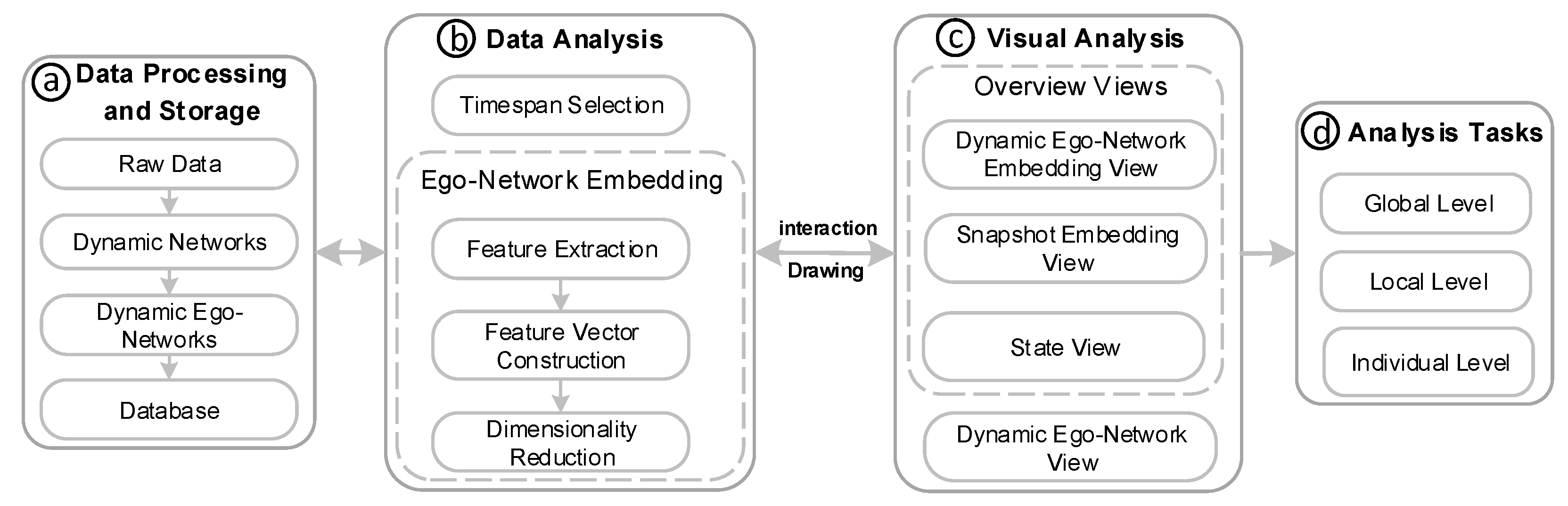
As shown in Figure 1, DyEgoVis implemented in the browser-server architecture has three main modules: data processing and storage module, data analysis module and visual analysis module. The first module aims to extract dynamic ego-networks from dynamic networks derived from temporal data. The extracted dynamic ego-networks are stored in the MongoDB database. As a core back-end component, the data analysis module is mainly used to generate the overview views (Figure 1c). After performing the process of the ego-network embedding, it can project the dynamic ego-networks in the specified timespan and their snapshots onto 2D views (i.e., overview views) where each point represents a dynamic ego-network or a snapshot. In overview views, clusters indicate similar evolution patterns (or states) while outliers represent uncommon evolution patterns (or states). The data analysis module was developed based on Python3 and Flask. It used the graph libraries NetworkX [40] and DyNetx to extract features and construct feature vectors. As a front-end component, the visual analysis module provides multiple views and smooth interactions to support the multilevel analysis of dynamic ego-networks. It was implemented based on Vue and D3 [41].
4. Visual Design and Implementation
4.1. Ego-Network Embedding
Using the ego-network embedding, we can reduce dynamic ego-networks and their snapshots to 2D points to generate overview views for users. The embedding pipeline has three stages: feature extraction, feature vector construction and dimensionality reduction. Below, we introduce this pipeline.
Feature Extraction. We need to select some features to characterize an ego-network (i.e., a snapshot) at timestep t. The studies on ego-networks or network similarity [4,35,42,43] have proposed many effective topological features. Based on our analytical tasks, we choose the following topological features for the ego-network:
- TF1: number of the ego u’s one-level alters.
- TF2: number of edges between one-level alters.
- TF3: clustering coefficient of the ego-network, computed as .
- TF4: average weight of edges (i.e., ego-alter edges) between the ego u and one-level alters, computed as , where is an ego-alter edge and indicates ’s weight.
- TF5: number of the ego u’s two-level alters.
- TF6: average degree of one-level alters, computed as , where is the degree of node i.
In addition to the above topological features, we can take the ego-network’s node attributes into consideration, which increases the possibility of clusters with semantic meanings in overview views.
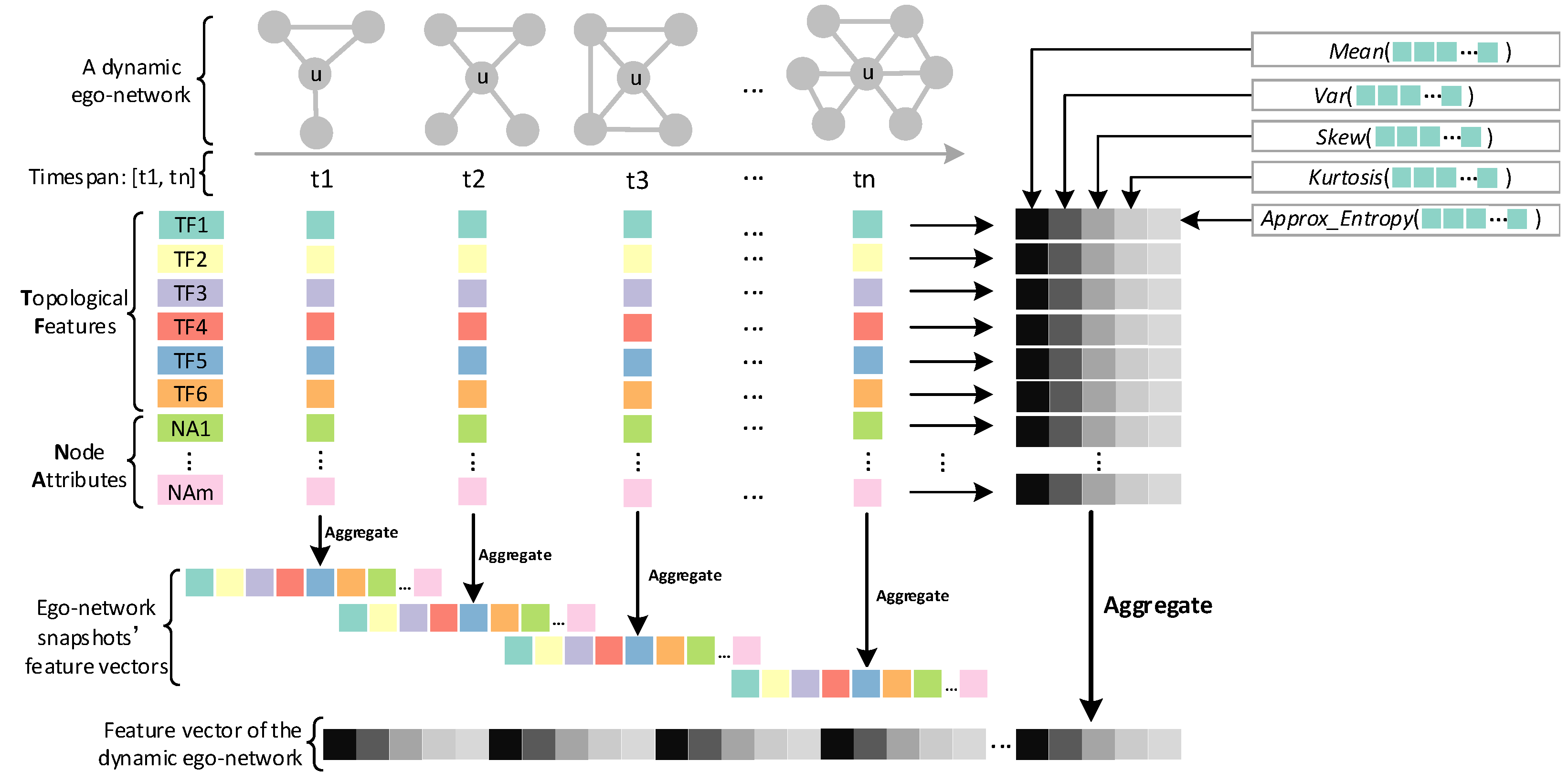
Feature Vector Construction. To tackle tasks T1 and T3, we need to construct a feature vector for each dynamic ego-network. However, for tasks T2 and T4, we need to construct a feature vector for each snapshot of a dynamic ego-network. Based on the extracted features, we propose an ego-network embedding model as shown in Figure 2. Besides the six topological features, the model can integrate node attributes, i.e., domain features depending on datasets, such as publication number per year in a dynamic co-authorship network. For each snapshot, we aggregate its extracted features into a vector as its feature vector. For the dynamic ego-network, we use corresponding feature sequences to describe it. If these feature sequences are directly aggregated into a single vector, dynamic ego-networks with different timespans will have different lengths of feature vectors. To solve this issue, we first calculate five metrics for each feature sequence: mean, variance, skewness, kurtosis, and approximate entropy. The first four metrics can characterize the distribution of the feature sequence. The approximate entropy [44] can quantify the complexity and predictability of the feature sequence. We then aggregate the above metrics of all feature sequences into a single vector as the dynamic ego-network’s final feature vector. Its length is where N is the number of features.
Based on the ego-network embedding model, we can obtain feature vectors of dynamic ego-networks and their snapshots. Next, we perform dimensionality reduction to project the feature vectors onto corresponding 2D views, thereby generating overview views. However, we should normalize feature vectors before dimensionality reduction because each feature has a different scale and unit. To adapt different dimensionality reduction methods, we provide two normalization methods: z-score and min-max. Z-score normalization transforms features per dimension to have zero mean and unit variance. Min-max normalization scales features per dimension to .
Dimensionality Reduction. To explore different datasets, we provide three dimensionality reduction methods as options: Principal Component Analysis (PCA) [45], MultiDimensional Scaling (MDS) [34] and t-distributed Stochastic Neighbor Embedding (t-SNE) [46]. As a widely used linear method, PCA offers faster computational performance. For both MDS and t-SNE, we adopt the Canberra Distance function [42] to calculate their distance matrices: , where both x and y are feature vectors and n denotes feature vector length. The Canberra Distance function is sensitive to small changes, which helps to detect clusters and outliers of dynamic ego-networks or snapshots. For PCA, we apply z-score normalization to normalize feature vectors. For both MDS and t-SNE, min-max normalization is the preferred choice because it helps to preserve outliers.
4.2. User Interface
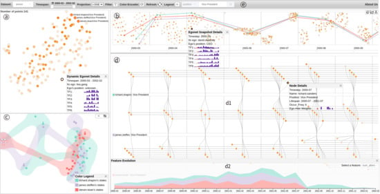
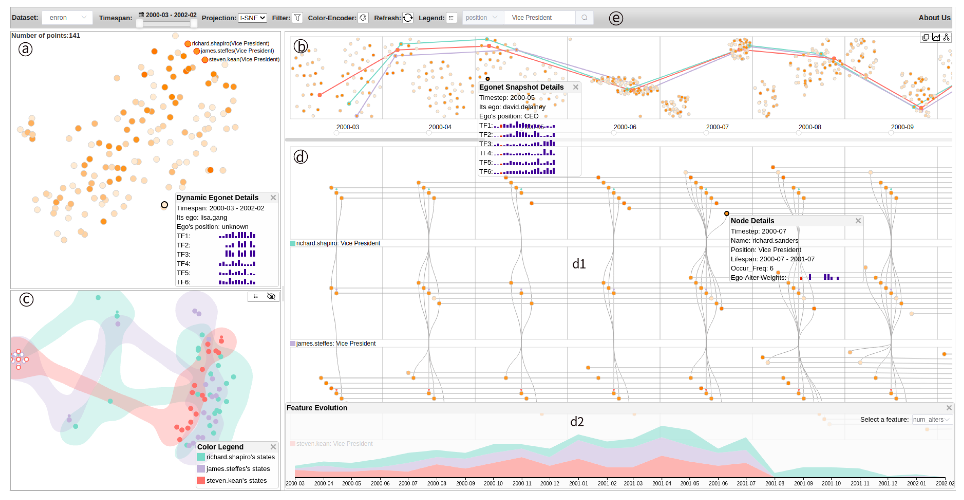
As shown in Figure 3, our system’s user interface mainly consists of five components: (a) a dynamic ego-network embedding view providing an overview of the evolution patterns of dynamic ego-networks, (b) a snapshot embedding view displaying the distribution of dynamic ego-networks at each timestep, (c) a state view showing an overview of all evolution states of the selected dynamic ego-networks, (d) a dynamic ego-network view displaying the layout of each selected dynamic ego-network and (e) a toolbar offering multiple system functions such as selecting a dataset, adjusting timespan, choosing a dimensionality reduction (projection) method and searching for egos of interest.
4.2.1. Dynamic Ego-Network Embedding View
This view (Figure 3a) summarizes the overall evolution patterns of dynamic ego-networks in a dynamic network (T1 and T3). Based on the selected projection method, the constructed feature vectors of the dynamic ego-networks are projected onto this 2D space where each point represents a dynamic ego-network. These feature vectors encode the evolution information of topology features and node attributes. If two dynamic ego-networks share similar evolution patterns, the distance between their feature vectors is small. Thus, the more similar the evolution patterns of two dynamic ego-networks are, the closer the corresponding points are. Clusters of points can reveal some common evolution patterns while outlier points indicate anomalous evolution patterns. The color of a point encodes an attribute of the ego of the corresponding dynamic ego-network such as the number of one-level alters. The greater the attribute value is, the darker the point’s color is. Users can select points of interest by clicking or lassoing to explore the corresponding dynamic ego-networks (Figure 3c,d). In addition, users can right-click on a point to see its details including attributes of the ego, small histograms of feature sequences, etc. The small histograms of feature sequences not only tell users what the evolutionary patterns of the dynamic ego-network are, but also interpret why the point is close to another point or why the point is an outlier.
4.2.2. Snapshot Embedding View
This view (Figure 3b) overviews the distribution of dynamic ego-networks at each timestep (T2 and T3). The feature vectors of the dynamic ego-networks’ snapshots are projected into the corresponding grids in which each dot indicates a snapshot. In each grid (i.e., a 2D space), the more similar two snapshots are, the closer the corresponding dots are. The dots in a cluster share similar characteristics while outliers have uncommon characteristics such as large numbers of one-level alters. The color darkness of each dot encodes the size of an attribute value of its ego. When the user hovers over a dot, the dots with the same ego are highlighted in red. If the user clicks a dot of interest, all the dots with the same ego are connected by lines with the same color so that the user tracks the distributions of the corresponding dynamic ego-network along the timeline. At the same time, the dynamic ego-network is displayed in the corresponding views (Figure 3c,d). Similarly, the user can right-click on a dot to inspect its details. In the details box, the position of the red small bar in the small histograms corresponds to the current timestep. The user can hover over each small bar to see its value and timestep.
4.2.3. State View
This view (Figure 3b) dispalys the evolution states of the selected dynamic ego-networks (T4). In this view, the feature vectors of the snapshots of the selected dynamic ego-networks are only projected onto a single 2D space where a point indicates a state (i.e., snapshot). Therefore, the states in different timesteps can be compared to find similar or abnormal ones. Closer points share similar states while outlying points have abnormal states. The points of the same dynamic ego-network not only share the same color but also are in a bubble [47] in the same color to distinguish different dynamic ego-networks (see the color legend in the lower right corner). When the user switches icon ![Applsci 11 02399 i001]() to icon
to icon ![Applsci 11 02399 i002]() in the upper right corner, all points of each dynamic ego-network are connected by lines with the corresponding colors along timesteps. Note that the points with circle dots at their top indicate the starting states while the ones with inverted triangles are the ending states. When the user hovers over a point, its previous state and next state are highlighted. Besides, the user can right-click on a point to see its details and click points of interest to locate the corresponding snapshots in dynamic ego-network view (Figure 3(b,d1)).
in the upper right corner, all points of each dynamic ego-network are connected by lines with the corresponding colors along timesteps. Note that the points with circle dots at their top indicate the starting states while the ones with inverted triangles are the ending states. When the user hovers over a point, its previous state and next state are highlighted. Besides, the user can right-click on a point to see its details and click points of interest to locate the corresponding snapshots in dynamic ego-network view (Figure 3(b,d1)).
 to icon
  in the upper right corner, all points of each dynamic ego-network are connected by lines with the corresponding colors along timesteps. Note that the points with circle dots at their top indicate the starting states while the ones with inverted triangles are the ending states. When the user hovers over a point, its previous state and next state are highlighted. Besides, the user can right-click on a point to see its details and click points of interest to locate the corresponding snapshots in dynamic ego-network view (Figure 3(b,d1)).
4.2.4. Dynamic Ego-Network View
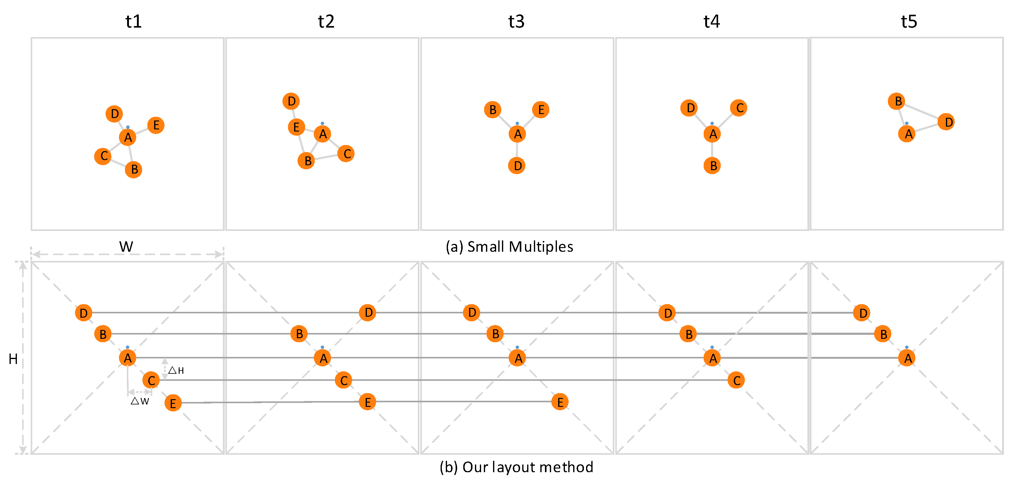
This view (Figure 3d) is designed to visualize and compare the selected dynamic ego-networks (T6–T11). As a typical dynamic network visualization method, small multiples can be used to visualize a dynamic ego-network as shown in Figure 4a. Based on the force-directed layout algorithm [41], each snapshot is drawn as a node-link diagram where the ego is marked by a colored dot at its top. Although this method can describe the structure of each snapshot well, the position of the same node in all snapshots is almost always different, making it difficult for users to track changes in ego-alter relationships. To address these issues, we propose a layout method suitable for analyzing the evolutions of ego–alter relationships, as shown in Figure 4b. In our layout, the ego is located in the center of a grid. The ego’s one-level alters are placed on the left diagonal of the grid while its one-level alters are placed on the right diagonal. Based on the task T9, we visualize only two-level alters that previously were one-level alters or subsequently became one-level alters, such as alter D in Figure 4b. The same nodes in all grids are connected by lines to allow users to track, compare and analyze the evolution of each alter. For example, in Figure 4b, alter B maintains a stable relationship with ego A; alter E has the shortest lifespan; and alter C disappears at timestep t3 and then reappears at timestep t4. The resulting layout should minimize line crossings and node overlapping to reduce visual clutter. In addition, long-life alters should be as close to the ego as possible. In our layout, the lifespan of an alter depends on its first and last appearances, regardless of whether it disappears during the period. Inspired by [2,48], our layout algorithm is shown in Algorithm 1. We input one-level alters and calculate their coordinates. When an alter changes from one-level to two-level, its current position should be horizontally aligned with the previous position as much as possible.
To reduce visual clutter, we hide the edges between nodes. However, when the user hovers over a node, all edges connected to it are displayed. If the user clicks an alter, its connection lines are highlighted in red. The user can right-click on a node to inspect its details such as lifespan, occurrence number and attributes. As shown in Figure 3(d1), if adjacent dynamic ego-networks have common nodes at a timestep, the common nodes are connected by curves to support task T11. The system allows the user to switch between our layout and small multiples layout by clicking on the icon ![Applsci 11 02399 i003]() in the upper right corner in Figure 3b. The user can click the icon
in the upper right corner in Figure 3b. The user can click the icon ![Applsci 11 02399 i004]() to decide whether to display two-level alters. To support task T5, we designed a feature evolution panel as shown in Figure 3(d2). This panel can be opened by clicking the icon
to decide whether to display two-level alters. To support task T5, we designed a feature evolution panel as shown in Figure 3(d2). This panel can be opened by clicking the icon ![Applsci 11 02399 i005]() . It adopts a stacked area chart to visualize the evolution of the specified feature of each selected dynamic ego-network. Note that when the user drags the timeline, both the snapshot embedding view and the dynamic ego-network view will move along with the timeline.
. It adopts a stacked area chart to visualize the evolution of the specified feature of each selected dynamic ego-network. Note that when the user drags the timeline, both the snapshot embedding view and the dynamic ego-network view will move along with the timeline.
 in the upper right corner in Figure 3b. The user can click the icon
  to decide whether to display two-level alters. To support task T5, we designed a feature evolution panel as shown in Figure 3(d2). This panel can be opened by clicking the icon
  . It adopts a stacked area chart to visualize the evolution of the specified feature of each selected dynamic ego-network. Note that when the user drags the timeline, both the snapshot embedding view and the dynamic ego-network view will move along with the timeline.
| Algorithm 1: Layout of a dynamic ego-network |
 |
4.2.5. Toolbar
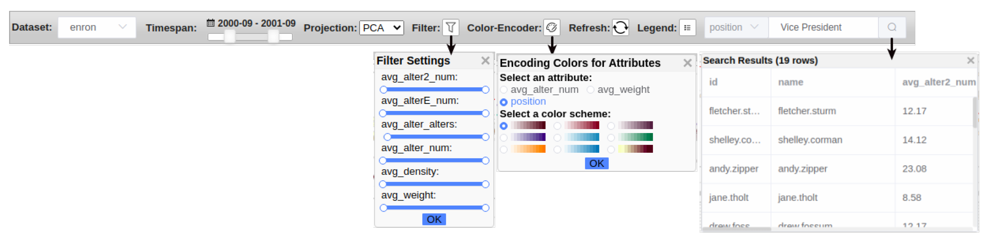
The toolbar (Figure 3e) allows users to access different system functions. After the user selects a dataset, the system first loads data from MongoDB and then performs a series of computations to generate the first two overview views (Figure 1c). At this time, the timespan slider shows the entire time span of the dataset. By adjusting the timespan slider, the user can obtain the overview views corresponding to the specified timespan to support task T3. PCA is the default projection method due to its fast performance. The user can also choose MDS or t-SNE to refresh the overview views (after clicking the refresh icon ![Applsci 11 02399 i007]() ). As shown in Figure 5, the user can click the filter icon
). As shown in Figure 5, the user can click the filter icon ![Applsci 11 02399 i008]() to pop up the filter settings dialog and then set the value interval of each feature to filter data. The user can select a color scheme from the color encoder to encode the selected attribute online. The user can also use the search box to search for target nodes and then explore the dynamic ego-networks of nodes of interest.
to pop up the filter settings dialog and then set the value interval of each feature to filter data. The user can select a color scheme from the color encoder to encode the selected attribute online. The user can also use the search box to search for target nodes and then explore the dynamic ego-networks of nodes of interest.
 ). As shown in Figure 5, the user can click the filter icon
  to pop up the filter settings dialog and then set the value interval of each feature to filter data. The user can select a color scheme from the color encoder to encode the selected attribute online. The user can also use the search box to search for target nodes and then explore the dynamic ego-networks of nodes of interest.
5. Case Studies
In this section, we demonstrate the usability and effectiveness of our system through two case studies on two real-world datasets: the Enron email network extracted from the Enron email dataset [49] and the TVCG co-authorship network extracted from TVCG publications.
5.1. Enron Email Network
Enron Corporation used to be a famous American energy company. However, it went bankrupt on 3 December 2001 due to financial scandals. The Enron email network is a dynamic network constructed based on Enron Corporation’s email dataset, consisting of 141 nodes and 4473 edges. It describes email exchanges (edges) among 141 employees (nodes) during the 24 months between March 2000 and February 2002. We take a month as a timestep. Therefore, an ego-network snapshot describes the email exchanges between the ego and other employees in the month. The weight of an edge in the snapshot is the number of email exchanges between its two nodes. In the entire network, the attributes of each node include the position, the number of monthly email contacts, the total number of monthly emails, etc. There are mainly ten positions from upper-level employees to low-level employees: CEO, President, Vice President, Director, Managing Director, Manager, In House Lawyer, Trader, Employee (junior employees) and Unknown (unknown employees).
After the system loads the data of the whole timespan (i.e., [March 2000, February 2002]), we select the color scheme ![Applsci 11 02399 i009]() to encode employees’ positions. The higher the position of an employee is, the darker the color of the corresponding node (or point) is. In this case study, one-level alters are more meaningful than two-level alters, so we show only one-level alters in the dynamic ego-network view.
to encode employees’ positions. The higher the position of an employee is, the darker the color of the corresponding node (or point) is. In this case study, one-level alters are more meaningful than two-level alters, so we show only one-level alters in the dynamic ego-network view.
 to encode employees’ positions. The higher the position of an employee is, the darker the color of the corresponding node (or point) is. In this case study, one-level alters are more meaningful than two-level alters, so we show only one-level alters in the dynamic ego-network view.
After learning that Enron’s stock price began to rise rapidly in July 2000 and continued to fall shortly thereafter, we adjust the timespan to [July 2000, February 2002] by using the timespan slider ![Applsci 11 02399 i010]() (T3). We select t-SNE as our project method and then click the refresh icon
(T3). We select t-SNE as our project method and then click the refresh icon ![Applsci 11 02399 i011]() to reload the data of the current timespan. The embedded results (points) of the dynamic ego-networks of 141 employees (as egos) are shown in Figure 6a. There is a small cluster (a1) in the view. Through examining the details of each point in this cluster, we find they have similar sparse feature sequences, as shown at the bottom in the view. This evolution pattern reveals that their egos did not communicate frequently with others between July 2000 and February 2002 (T1). Next, we want to investigate Enron’s senior executives. With the help of the system’s search box, we find the four CEOs: Kenneth Lay (founder of Enron), Jeff Skilling (second in command of Enron), David Delainey (CEO of Enron North America) and John Lavorato (CEO of Enron America). However, the embedded results of their dynamic ego-networks (highlighted in red) are far away from each other (Figure 6a). This means that their dynamic ego-networks have different evolution patterns (T1). In addition, this can reflect that these CEOs play different roles in the company’s decision-making.
to reload the data of the current timespan. The embedded results (points) of the dynamic ego-networks of 141 employees (as egos) are shown in Figure 6a. There is a small cluster (a1) in the view. Through examining the details of each point in this cluster, we find they have similar sparse feature sequences, as shown at the bottom in the view. This evolution pattern reveals that their egos did not communicate frequently with others between July 2000 and February 2002 (T1). Next, we want to investigate Enron’s senior executives. With the help of the system’s search box, we find the four CEOs: Kenneth Lay (founder of Enron), Jeff Skilling (second in command of Enron), David Delainey (CEO of Enron North America) and John Lavorato (CEO of Enron America). However, the embedded results of their dynamic ego-networks (highlighted in red) are far away from each other (Figure 6a). This means that their dynamic ego-networks have different evolution patterns (T1). In addition, this can reflect that these CEOs play different roles in the company’s decision-making.
 (T3). We select t-SNE as our project method and then click the refresh icon
  to reload the data of the current timespan. The embedded results (points) of the dynamic ego-networks of 141 employees (as egos) are shown in Figure 6a. There is a small cluster (a1) in the view. Through examining the details of each point in this cluster, we find they have similar sparse feature sequences, as shown at the bottom in the view. This evolution pattern reveals that their egos did not communicate frequently with others between July 2000 and February 2002 (T1). Next, we want to investigate Enron’s senior executives. With the help of the system’s search box, we find the four CEOs: Kenneth Lay (founder of Enron), Jeff Skilling (second in command of Enron), David Delainey (CEO of Enron North America) and John Lavorato (CEO of Enron America). However, the embedded results of their dynamic ego-networks (highlighted in red) are far away from each other (Figure 6a). This means that their dynamic ego-networks have different evolution patterns (T1). In addition, this can reflect that these CEOs play different roles in the company’s decision-making.
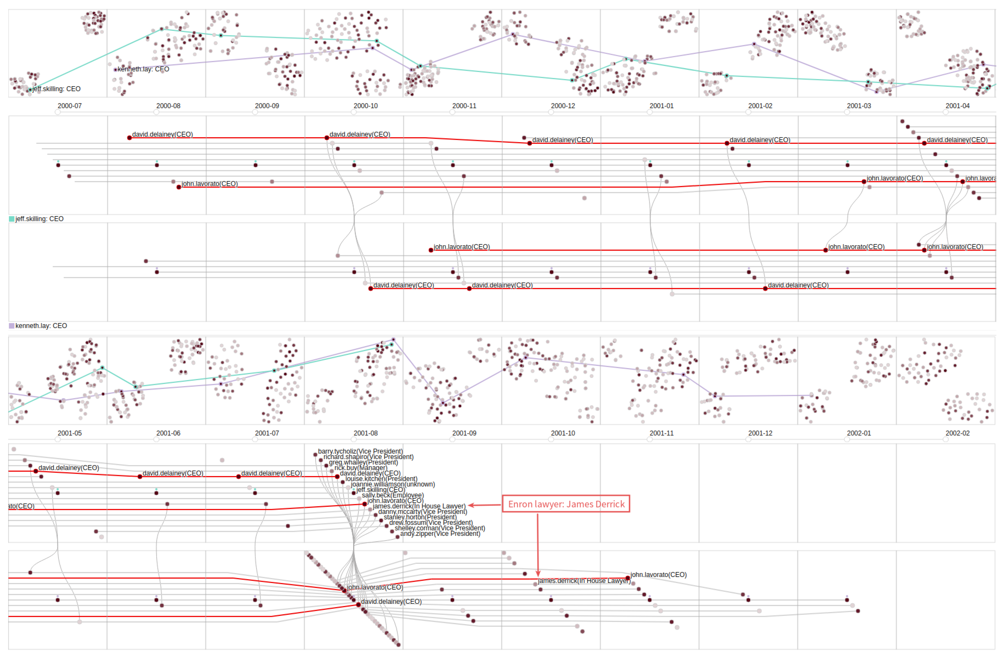
We then focus on the dynamic ego-networks of the two most influential CEOs Jeff Skilling and Kenneth Lay to get insight into their relationships with others. All the states of their dynamic ego-networks are shown in Figure 6b. We notice that Kenneth Lay’s state b2 in August 2001 is an apparent outlier. The timesteps of the states b1 and b3 are July 2001 and September 2001, respectively. The state sequence b1-b2-b3 reveals that Kenneth Lay’s dynamic ego-network changed dramatically between July 2001 and September 2001 (T4). To further understand these states, we drag the timeline to investigate the layouts of the corresponding snapshots in the dynamic ego-network view. As shown in Figure 7, Kenneth Lay (row 6, col 4) communicated with a large number of employees (i.e., one-level alters) via email in August 2001. Similarly, Jeff Skilling (row 5, col 4) also contacted many senior executives. According to Enron Company’s profile, we learn that Jeff Skilling succeeded Kenneth Lay as CEO in February 2001. However, he suddenly resigned in August 2001 and Kenneth Lay took over again. The above abnormal changes are caused by this incident (T7).
From the results in the snapshot embedding view (rows 1 and 4 in Figure 7), we find there are only two large clusters at most timesteps (T2). Along the timeline, we discover that Jeff Skilling’s and Kenneth Lay’s ego-network snapshots locate in the same clusters from time to time. This reveals that the two CEOs had similar ego-network snapshots (states) at the corresponding timesteps such as October 2000, November 2000 and August 2001.
From the layout results (rows 2, 3, 5 and 6 in Figure 7), we observe that Jeff Skilling and Kenneth Lay have some common one-level alters (connected by curves) while there are no email exchanges between them (T11). The other two CEOs, David Delainey and John Lavorato, are also their common one-level alters. To track and analyze the relationships among the four CEOs, we click David Delainey and John Lavorato to highlight their nodes with red connection lines. Both David Delainey and John Lavorato first joined Jeff Skilling’s dynamic ego-network in August 2000 (T8). However, David Delainey had more frequent contacts with Jeff Skilling. John Lavorato served as a bridge node between Jeff Skilling and Kenneth Lay because he often appeared simultaneously in their ego-network snapshots. In April 2001, Jeff Skilling suddenly communicated with many upper-level employees including David Delainey and John Lavorato. We infer this may be caused by the incident that Jeff Skilling verbally attacked Wall Street Analyst Richard Grubman who questioned Enron’s unusual accounting practice.
Another common one-level alter James Derrick (In House Lawyer), former Enron general counsel, catches our attention. To further analyze his relationships with others, we display and examine his dynamic ego-network. As shown in Figure 8, he first appeared in July 2000 and disappeared after Enron filed for bankruptcy (T8). In this period, he mainly had two stable one-level alters (highlighted with red connection lines). One was Richard Sanders who served as Enron Vice President and assistant general counsel. The other was J. Harris who was an unknown employee. From the histogram in J. Harris’s node details box, we are surprised to find 83 email exchanges (the red bar) between him and James Derrick in Oct. 2001 (T10). This may be due to the SEC (U.S. Securities and Exchange Commission) investigation. Based on J. Harris’s behaviors, we infer that J. Harris may be an in-house lawyer.
5.2. TVCG Co-Authorship Network
TVCG (IEEE Transactions on Visualization and Computer Graphics) is the top journal in the field of visualization. We first extracted a collection of TVCG papers published between 1995 and 2019 from the DBLP dataset and then constructed a dynamic TVCG co-authorship network based on these papers. It spans the 25 years between 1995 and 2019 and contains 8158 authors (nodes) and 26,685 collaboration relationships (edges). We take a year as a timestep. The weight of an edge in each ego-network snapshot represents the number of papers co-authored by its two authors in the year. The attributes of each author include the number of TVCG papers per year, the total number of TVCG papers, research interests, affiliations, the total number of collaborators, etc. In the feature vector construction, we consider the number of TVCG papers per year (denoted as NA1).
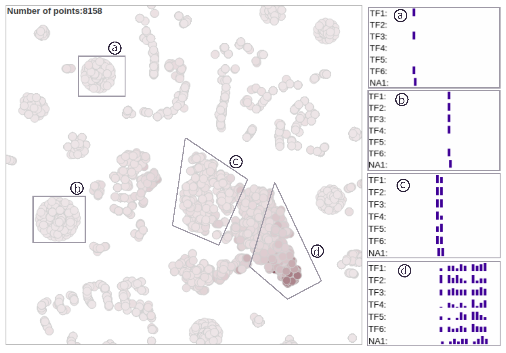
We select t-SNE as our projection method and load the data of the entire timespan [1995, 2019]. The same color scheme ![Applsci 11 02399 i012]() is used to encode the total number of TVCG papers of each author. The more TVCG papers an author (or ego) has, the darker the corresponding node (or point) is. In this case study, we consider one-level and two-level alters so that we can explore the changes in ego-alter relationships. The embedded results (points) of the dynamic ego-networks of 8158 authors (as egos) are shown in Figure 9. There are many clusters in the view. We choose four dense clusters (a, b, c, d) to explore the corresponding evolution patterns. The general feature sequences of each cluster are shown on the right in Figure 9. Each group of feature sequences, as an interpretation of the corresponding cluster, can reveal the common evolution pattern of dynamic ego-networks in the cluster (T1). In clusters a and a, each dynamic ego-network has only one snapshot and the ego of each dynamic ego-network only published a TVCG paper. Through comparing their feature TF1, we find that each ego in cluster a has only a coauthor while each ego in cluster b has two co-authors. In cluster c, each ego typically published two TVCG papers within five years and each of the two papers has more than two co-authors. Therefore, we infer that almost all the egos in clusters a, b and c were students. In cluster d, each dynamic ego-network has continuous multiple ego-network snapshots, which means each ego has published papers in TVCG for multiple years. Most of the egos in cluster d are long-term visualization researchers who have higher publication performance. They have a more significant impact on the field of visualization.
is used to encode the total number of TVCG papers of each author. The more TVCG papers an author (or ego) has, the darker the corresponding node (or point) is. In this case study, we consider one-level and two-level alters so that we can explore the changes in ego-alter relationships. The embedded results (points) of the dynamic ego-networks of 8158 authors (as egos) are shown in Figure 9. There are many clusters in the view. We choose four dense clusters (a, b, c, d) to explore the corresponding evolution patterns. The general feature sequences of each cluster are shown on the right in Figure 9. Each group of feature sequences, as an interpretation of the corresponding cluster, can reveal the common evolution pattern of dynamic ego-networks in the cluster (T1). In clusters a and a, each dynamic ego-network has only one snapshot and the ego of each dynamic ego-network only published a TVCG paper. Through comparing their feature TF1, we find that each ego in cluster a has only a coauthor while each ego in cluster b has two co-authors. In cluster c, each ego typically published two TVCG papers within five years and each of the two papers has more than two co-authors. Therefore, we infer that almost all the egos in clusters a, b and c were students. In cluster d, each dynamic ego-network has continuous multiple ego-network snapshots, which means each ego has published papers in TVCG for multiple years. Most of the egos in cluster d are long-term visualization researchers who have higher publication performance. They have a more significant impact on the field of visualization.
 is used to encode the total number of TVCG papers of each author. The more TVCG papers an author (or ego) has, the darker the corresponding node (or point) is. In this case study, we consider one-level and two-level alters so that we can explore the changes in ego-alter relationships. The embedded results (points) of the dynamic ego-networks of 8158 authors (as egos) are shown in Figure 9. There are many clusters in the view. We choose four dense clusters (a, b, c, d) to explore the corresponding evolution patterns. The general feature sequences of each cluster are shown on the right in Figure 9. Each group of feature sequences, as an interpretation of the corresponding cluster, can reveal the common evolution pattern of dynamic ego-networks in the cluster (T1). In clusters a and a, each dynamic ego-network has only one snapshot and the ego of each dynamic ego-network only published a TVCG paper. Through comparing their feature TF1, we find that each ego in cluster a has only a coauthor while each ego in cluster b has two co-authors. In cluster c, each ego typically published two TVCG papers within five years and each of the two papers has more than two co-authors. Therefore, we infer that almost all the egos in clusters a, b and c were students. In cluster d, each dynamic ego-network has continuous multiple ego-network snapshots, which means each ego has published papers in TVCG for multiple years. Most of the egos in cluster d are long-term visualization researchers who have higher publication performance. They have a more significant impact on the field of visualization.
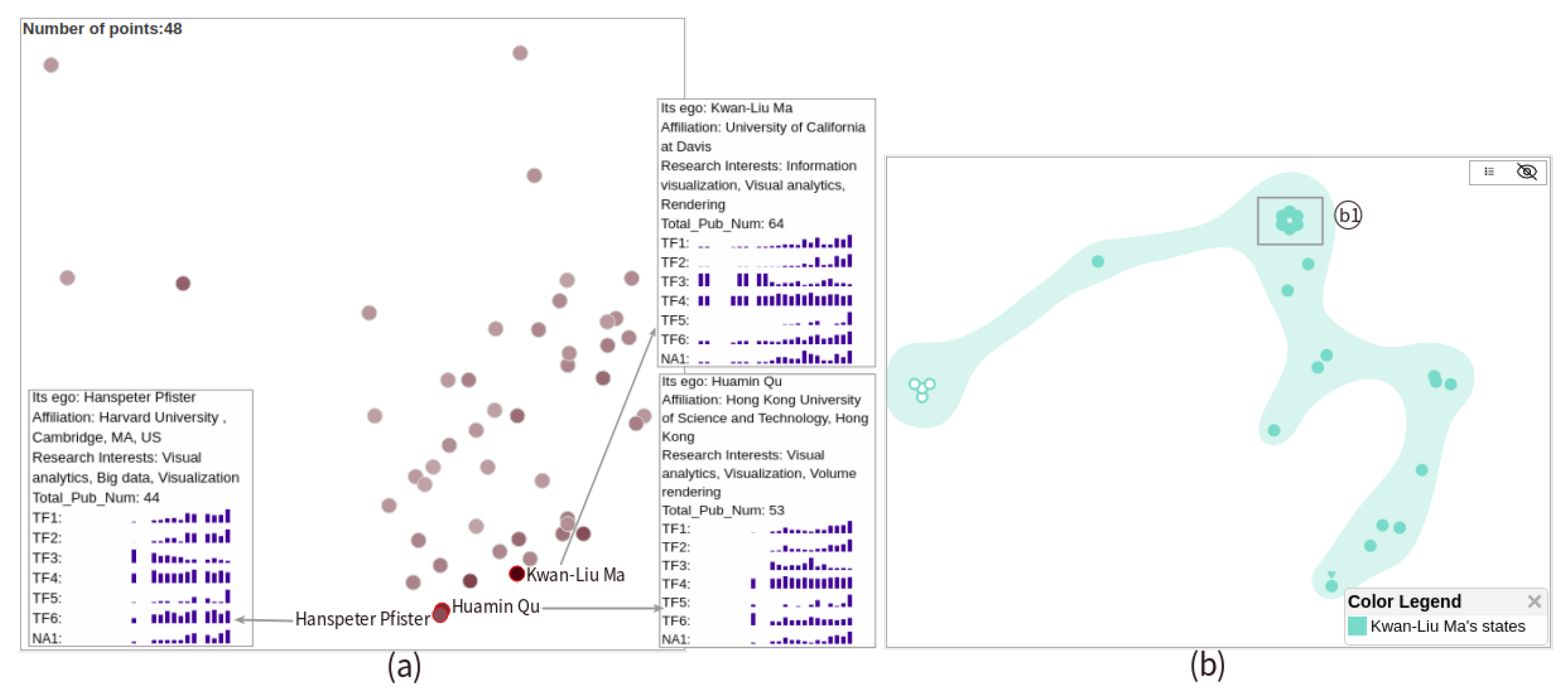
Next, we focus on authors who have high publication performance. We used the system’s filter (Figure 5) to obtain the embedded results of the dynamic ego-networks of the authors who have published at least 20 TVCG papers, as shown in Figure 10a. The darkest point corresponds to Kwan-Liu Ma’s dynamic ego-network. Ma has the most TVCG papers (64 in total). The two overlapping dark points correspond to Huamin Qu’s and Hanspeter Pfister’s dynamic ego-networks respectively. Huamin Qu and Hanspeter Pfister have highly similar feature sequences as shown in the details boxes in Figure 10a. Besides, they have similar research interests (T1).
We first explore the evolution of Kwan-Liu Ma’s dynamic ego-network to analyze his academic career. As shown in Figure 10b, there is a dense cluster (b1) in the state view of his dynamic ego-network (T4). The points in this cluster revealed that Ma had similar states (ego-networks) in his early academic years (1996–2006). We can verify this through inspecting his feature sequences (Figure 10a). We then analyze his dynamic ego-network shown in Figure 11a. During 1996–2006, Ma had a small number of collaborators and was absent from TVCG for four years (1998–2000 and 2004). From his profile, we know that he was a staff scientist at ICASE during 1993–1999 and has been at UC Davis since July 1999. As shown in Figure 11b, he published a TVCG paper almost every year between 2001 and 2006. After 2007, the number of his TVCG papers increased with the number of his collaborators. He maintained a high publication performance (more than three TVCG papers) for many years (T5). We define a coauthor who has collaborated with the ego for at least five years as a long-term collaborator. Through interactive analysis of Ma’s dynamic ego-network (Figure 11a), we discover some interest alters (highlighted with red lines). Ma’s one-level alter C.D. Correa was his only long-term collaborator. The one-level alter Wei Chen (a professor at Zhejiang University, China) has maintained a collaborative relationship with Ma for four years since 2014. There are several alters that became two-level from one-level, such as Yingcai Wu who was a postdoc at UC Davis during 2010–2012 and has been at Zhejiang University since 2015, and Ying Zhao who is a researcher at Central South University, China. Panpan Xu is the only alter that became one-level from two-level (T9). In 2013, she collaborated with Yingcai Wu while Yingcai Wu was a coauthor of Ma. Based on the above analysis, we can find that Ma has relatively frequent cross-institutional collaborations with Chinese visualization researchers.
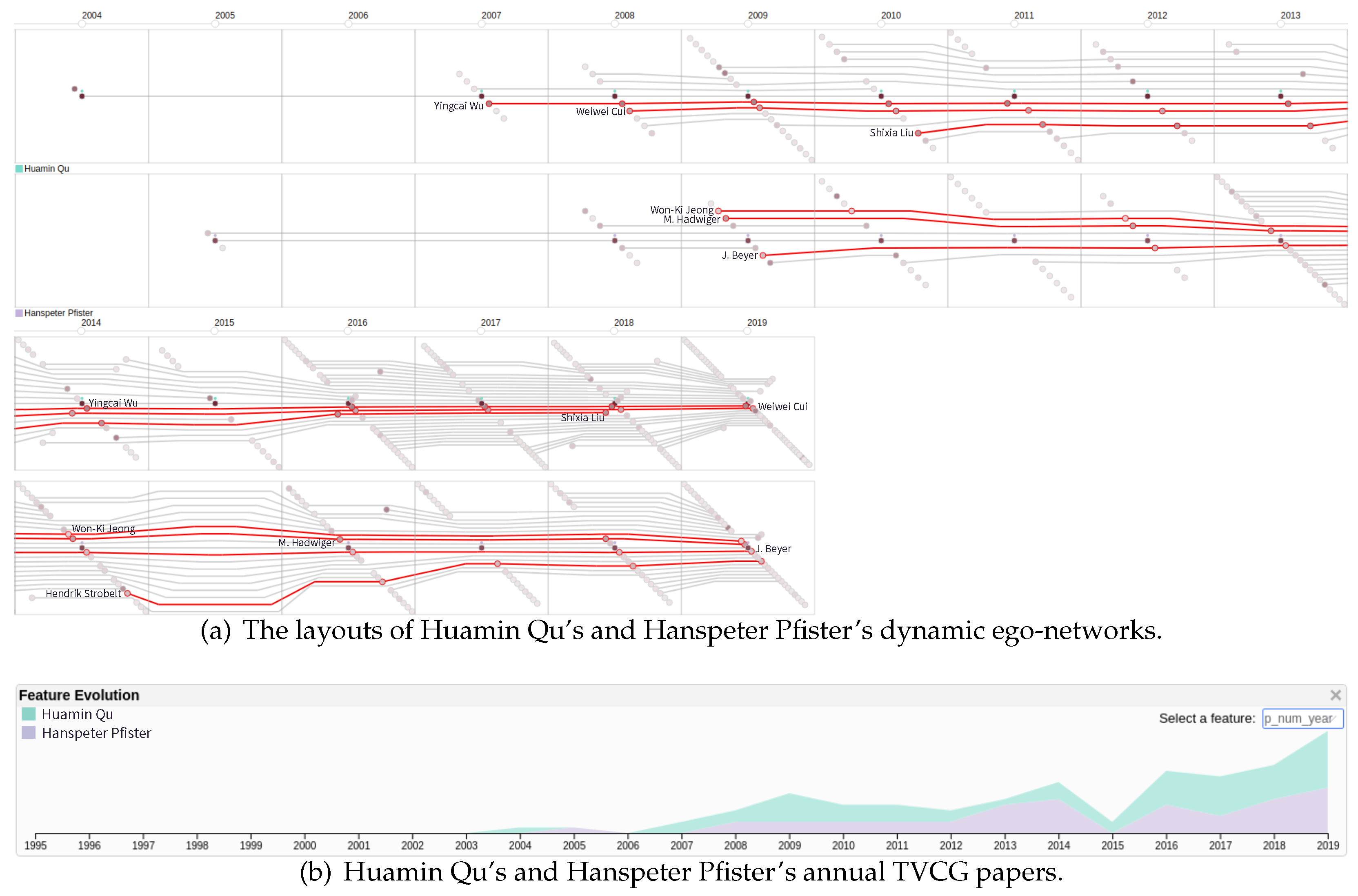
We then compare and analyze the evolutions of Huamin Qu’s and Hanspeter Pfister’s dynamic ego-networks. From the profiles of the two researchers, we learn about their experiences. Qu received his PhD from Stony Brook University in 2004 and has been at the Hong Kong University of Science and Technology since 2005. After receiving PhD (1996) from Stony Brook University, Pfister worked at MERL for over a decade and then joined Harvard University in 2007. As shown in Figure 12a,b, their academic careers are similar in general. They both published a TVCG paper in their early years. After a two-year absence from TVCG, they both entered a period of rapid growth in their academic careers (T5). Through further comparison, we also find some differences between them. Qu has three long-term collaborators: Yingcai Wu, Weiwei Cui and Shixia Liu. The first two were his PhD students. After they graduated, they still maintained long-term cooperative relationships with Qu. Shixia Liu often cooperated with Qu during her time at MSRA (2010–2014). Pfister has four long-term collaborators: Won-Ki Jeong, M. Hadwiger, J. Beyer and Hendrik Strobelt. As a researcher at KAUST, M. Hadwiger maintained cross-institutional collaborations with Pfister. However, the other three collaborators (postdoctoral fellows at Harvard University) had intra-institutional collaborations with Pfister. In 2015, Pfister had no TVCG papers. From his website, we find that he published multiple top conference papers on computer vision in the year. In addition to the above differences, we observe that Qu has more two-level alters, especially in recent years (T7). This reflects Qu’s growing influence in the field of visualization.
6. Discussion and Future Work
In our system, the ego-network embedding model (Figure 2) is essential for generating the overview views. It can construct feature vectors for dynamic ego-networks and their snapshots based on topological features and node attributes. In this paper, the model considers six topological features that can comprehensively describe an ego-network. We want to verify whether the constructed feature vectors can characterize their dynamic ego-network well. This can be done by projecting them onto a 2D view. If a set of similar dynamic ego-networks are clustered together while the anomalous dynamic ego-networks are outliers, their feature vectors can be verified to be effective. In the first case study, we can verify that the feature vectors of snapshots are effective (see the caption of Figure 8). In the second case study, we can verify that the feature vectors of dynamic ego-networks are effective (see the caption of Figure 12). Thus, we demonstrate the effectiveness of the ego-network embedding model in the two case studies. However, real-world datasets are usually complex, e.g., having hundreds of timesteps and numerous node attributes. We plan to further demonstrate the effectiveness of the model on datasets from different domains.
Compared to the small multiple layout, our layout can maintain the positions of alters as much as possible to allow users to track, compare and analyze the changes in ego-alter relationships. Through the two case studies, we can demonstrate the effectiveness of our layout. In the small mutiple layout, we can easily find some communities of alters in a snapshot. This can help users understand the components of an ego-network. Thus, we plan to improve our layout method so that alters in the same community are grouped together. In addition, we want to add the Fisheye interaction to help users inspect dense alters.
The system’s computation time is mainly spent on the embedding pipeline. The pipeline consists of three stages: feature extraction, feature vector construction and dimensionality reduction. The first stage can be done offline. The extracted feature sequences are stored in the database. When the user selects a timespan of interest by adjusting the timespan slider (Figure 5), the second stage is rerun to construct feature vectors for dynamic ego-networks of the selected timespan. However, the constructed feature vectors can be stored in a local file as a cache. For the third stage, we provide three typical methods as options: PCA, MDS and t-SNE. In our case studies, the nonlinear methods MDS and t-SNE worked much better than the linear method PCA for clustering on dynamic ego-networks. This is likely because both MDS and t-SNE do better than PCA in preserving small distances between feature vectors. Overall, the system’s computational scalability is most limited by MDS and t-SNE, while PCA runs in only seconds. In addition, our system provides a filter function (Figure 5). On the one hand, it can filter out irrelevant data to reduce visual clutter. On the other hand, it can also improve the computational scalability of the system to allow users to explore larger datasets.
In this paper, we conducted two case studies to demonstrate the effectiveness of DyEgoVis. In the future, we want to conduct a user study to collect more feedback on our system. Besides, we aim to further examine the effectiveness of DyEgoVis by conducting more case studies with datasets from different domains.
7. Conclusions
We present DyEgoVis, an interactive visualization system for exploring dynamic ego-networks, which provides multiple interactive overview views and a new layout design to tackle the tasks at the three analysis levels: global, local and individual. We propose an ego-network embedding model which is integrated into DyEgoVis to generate overview views. The overview views summarize the evolution patterns of dynamic ego-networks and the evolution states of the selected dynamic ego-networks across different timesteps. We devise a new layout for the selected dynamic ego-networks to help users track, compare and analyze the changes of ego-alter relationships. We describe two case studies on real datasets. The results suggest that DyEgoVis is effective and useful for the analysis of dynamic ego-network evolution.
Author Contributions
Conceptualization, T.M., K.F. and Y.W.; Data curation, T.M., D.L. and Y.Z.; Formal analysis, T.M., Y.W. and Y.Z.; Investigation, T.M.; Methodology, T.M., K.F., Y.W. and D.L.; Software, T.M. and Y.Z.; Supervision, K.F., Y.W. and X.S.; Validation, T.M., K.F. and Y.W.; Visualization, all authors; Writing—original draft, T.M.; Writing—review & editing, T.M., K.F. and Y.W. All authors have read and agreed to the published version of the manuscript.
Funding
This research was funded by the National Natural Science Foundation of China, grant number 61725105.
Acknowledgments
The authors would like to thank all the colleagues for the fruitful discussions on dynamic network visualization.
Conflicts of Interest
The authors declare no conflict of interest.
References
- Chung, K.; Hossain, L.; Davis, J. Exploring Sociocentric and Egocentric Approaches for Social Network Analysis. In Proceedings of the 2005 International Conference on Knowledge Management, Wellington, New Zealand, 27–28 October 2005. [Google Scholar]
- Zhao, J.; Glueck, M.; Chevalier, F.; Wu, Y.; Khan, A. Egocentric analysis of dynamic networks with egolines. In Proceedings of the 2016 CHI Conference on Human Factors in Computing Systems, San Jose, CA, USA, 7–12 May 2016; pp. 5003–5014. [Google Scholar]
- Lei, S.; Chen, W.; Zhen, W.; Huamin, Q.; Chuang, L.; Qi, L. 1.5D Egocentric Dynamic Network Visualization. IEEE Trans. Vis. Comput. Graph. 2015, 21, 624–637. [Google Scholar]
- Wu, Y.; Pitipornvivat, N.; Zhao, J.; Yang, S.; Huang, G.; Qu, H. egoslider: Visual analysis of egocentric network evolution. IEEE Trans. Vis. Comput. Graph. 2015, 22, 260–269. [Google Scholar] [CrossRef]
- Kikas, R.; Dumas, M.; Karsai, M. Bursty egocentric network evolution in Skype. Soc. Netw. Anal. Min. 2013, 3, 1393–1401. [Google Scholar] [CrossRef] [Green Version]
- Shneiderman, B. The eyes have it: A task by data type taxonomy for information visualizations. In The Craft of Information Visualization; Elsevier: Amsterdam, The Netherlands, 2003; pp. 364–371. [Google Scholar]
- Beck, F.; Burch, M.; Diehl, S.; Weiskopf, D. A Taxonomy and Survey of Dynamic Graph Visualization. Comput. Graph. Forum 2017, 36, 133–159. [Google Scholar] [CrossRef]
- Hadlak, S.; Schumann, H.; Schulz, H.J. A Survey of Multi-faceted Graph Visualization. In Proceedings of the 17th Eurographics Conference on Visualization, EuroVis 2015 - State of the Art Reports, Cagliari, Sardinia, Italy, 25–29 May 2015. [Google Scholar]
- Kerracher, N.; Kennedy, J.; Chalmers, K. A Task Taxonomy for Temporal Graph Visualisation. IEEE Trans. Vis. Comput. Graph. 2015, 21, 1160–1172. [Google Scholar] [CrossRef]
- Eades, P.; Huang, M. Navigating Clustered Graphs Using Force-Directed Methods. J. Graph Algorithms Appl. 2000, 4, 157–181. [Google Scholar] [CrossRef] [Green Version]
- Yee, K.; Fisher, D.; Dhamija, R.; Hearst, M.A. Animated exploration of dynamic graphs with radial layout. In Proceedings of the IEEE Symposium on Information Visualization 2001 (INFOVIS’01), San Diego, CA, USA, 22–23 October 2001. [Google Scholar]
- Bach, B.; Pietriga, E.; Fekete, J.D. GraphDiaries: Animated Transitions andTemporal Navigation for Dynamic Networks. IEEE Trans. Vis. Comput. Graph. 2014, 20, 740–754. [Google Scholar] [CrossRef]
- Crnovrsanin, T.; Shilpika; Chandrasegaran, S.; Ma, K.L. Staged Animation Strategies for Online Dynamic Networks. IEEE Trans. Vis. Comput. Graph. 2021, 27, 539–549. [Google Scholar] [CrossRef]
- Hong, S.; Eades, P.; Torkel, M.; Huang, W.; Cifuentes, C. Dynamic Graph Map Animation. In Proceedings of the 2020 IEEE Pacific Visualization Symposium, PacificVis 2020, Tianjin, China, 3–5 June 2020. [Google Scholar] [CrossRef]
- Elzen, S.V.D.; Wijk, J.V. Small Multiples, Large Singles: A New Approach for Visual Data Exploration. Comput. Graph. Forum 2013, 32, 191–200. [Google Scholar] [CrossRef]
- Bach, B.; Riche, N.; Dwyer, T.; Madhyastha, T.; Fekete, J.D.; Grabowski, T. Small MultiPiles: Piling Time to Explore Temporal Patterns in Dynamic Networks. Comput. Graph. Forum 2015, 34, 31–40. [Google Scholar] [CrossRef] [Green Version]
- Wang, Y.; Archambault, D.W.; Haleem, H.; Möller, T.; Wu, Y.; Qu, H. Nonuniform Timeslicing of Dynamic Graphs Based on Visual Complexity. In Proceedings of the 30th IEEE Visualization Conference, IEEE VIS 2019 - Short Papers, Vancouver, BC, Canada, 20–25 October 2019. [Google Scholar]
- Cakmak, E.; Schlegel, U.; Jäckle, D.; Keim, D.; Schreck, T. Multiscale Snapshots: Visual Analysis of Temporal Summaries in Dynamic Graphs. IEEE Trans. Vis. Comput. Graph. 2020, 27, 517–527. [Google Scholar] [CrossRef]
- Bach, B.; Shi, C.; Heulot, N.; Madhyastha, T.M.; Grabowski, T.J.; Dragicevic, P. Time Curves: Folding Time to Visualize Patterns of Temporal Evolution in Data. IEEE Trans. Vis. Comput. Graph. 2016, 22, 559–568. [Google Scholar] [CrossRef] [Green Version]
- Elzen, S.V.D.; Holten, D.; Blaas, J.; Wijk, J.J.V. Reducing Snapshots to Points: A Visual Analytics Approach to Dynamic Network Exploration. IEEE Trans. Vis. Comput. Graph. 2015, 22, 1. [Google Scholar] [CrossRef]
- Hajij, M.; Wang, B.; Scheidegger, C.; Rosen, P. Visual Detection of Structural Changes in Time-Varying Graphs Using Persistent Homology. In Proceedings of the IEEE Pacific Visualization Symposium, PacificVis 2018, Kobe, Japan, 10–13 April 2018. [Google Scholar]
- Arendt, D.; Blaha, L.M. SVEN: Informative Visual Representation of Complex Dynamic Structure. arXiv 2014, arXiv:abs/1412.6706. [Google Scholar]
- Bach, B.; Pietriga, E.; Fekete, J.D. Visualizing Dynamic Networks with Matrix Cubes. In Proceedings of the CHI Conference on Human Factors in Computing Systems, CHI’14, Toronto, ON, Canada, 26 April–1 May 2014. [Google Scholar]
- Bach, B.; Kerracher, N.; Hall, K.; Carpendale, M.S.T.; Kennedy, J.; Riche, N. Telling Stories about Dynamic Networks with Graph Comics. In Proceedings of the 2016 CHI Conference on Human Factors in Computing Systems, San Jose, CA, USA, 7–12 May 2016. [Google Scholar]
- Burch, M.; Hlawatsch, M.; Weiskopf, D. Visualizing a Sequence of a Thousand Graphs (or Even More). Comput. Graph. Forum 2017, 36. [Google Scholar] [CrossRef]
- Pham, V.; Nguyen, V.N.; Dang, T. DualNetView: Dual Views for Visualizing the Dynamics of Networks. In Proceedings of the 11th International EuroVis Workshop on Visual Analytics, EuroVA@Eurographics/EuroVis 2020, Norrköping, Sweden, 25 May 2020. [Google Scholar]
- Rufiange, S.; McGuffin, M. DiffAni: Visualizing Dynamic Graphs with a Hybrid of Difference Maps and Animation. IEEE Trans. Vis. Comput. Graph. 2013, 19, 2556–2565. [Google Scholar] [CrossRef] [PubMed] [Green Version]
- Hadlak, S.; Schulz, H.J.; Schumann, H. In Situ Exploration of Large Dynamic Networks. IEEE Trans. Vis. Comput. Graph. 2011, 17, 2334–2343. [Google Scholar] [CrossRef]
- Lee, A.; Archambault, D.W.; Nacenta, M.A. Dynamic Network Plaid: A Tool for the Analysis of Dynamic Networks. In Proceedings of the 2019 CHI Conference on Human Factors in Computing Systems, CHI 2019, Glasgow, Scotland, UK, 4–9 May 2019. [Google Scholar]
- Reitz, F. A Framework for an Ego-centered and Time-aware Visualization of Relations in Arbitrary Data Repositories. arXiv 2010, arXiv:1009.5183. [Google Scholar]
- Farrugia, M.; Hurley, N.; Quigley, A. Exploring temporal ego networks using small multiples and tree-ring layouts. Proc. ACHI 2011, 2011, 23–28. [Google Scholar]
- Liu, Q.; Hu, Y.; Lei, S.; Mu, X.; Zhang, Y.; Jie, T. EgoNetCloud: Event-based egocentric dynamic network visualization. In Proceedings of the IEEE Conference on Visual Analytics Science & Technology, Chicago, IL, USA, 25–30 October 2015. [Google Scholar]
- Boz, H.A.; Bahrami, M.; Suhara, Y.; Bozkaya, B.; Balcisoy, S. An Exploratory Visual Analytics Tool for Multivariate Dynamic Networks. In EuroVis Workshop on Visual Analytics (EuroVA); Turkay, C., Vrotsou, K., Eds.; The Eurographics Association: Geneve, Switzerland, 2020. [Google Scholar] [CrossRef]
- Kruskal, J. Multidimensional scaling by optimizing goodness of fit to a nonmetric hypothesis. Psychometrika 1964, 29, 1–27. [Google Scholar] [CrossRef]
- Lu, B.; Zhu, M.; He, Q.; Li, M.; Jia, R. TMNVis: Visual Analysis of Evolution in Temporal Multivariate Network at Multiple Granularities. J. Vis. Lang. Comput. 2017, 43, S1045926X16301458. [Google Scholar] [CrossRef]
- He, Q.; Zhu, M.; Lu, B.; Liu, H.; Shen, Q. MENA: Visual Analysis of Multivariate Egocentric Network Evolution. In Proceedings of the International Conference on Virtual Reality & Visualization, Zhengzhou, China, 21–22 October 2017. [Google Scholar]
- Freire, M.; Plaisant, C.; Shneiderman, B.; Golbeck, J. ManyNets: An interface for multiple network analysis and visualization. In Proceedings of the 28th International Conference on Human Factors in Computing Systems, CHI 2010, Atlanta, GA, USA, 10–15 April 2010. [Google Scholar]
- Law, P.M.; Wu, Y.; Basole, R.C. Segue: Overviewing Evolution Patterns of Egocentric Networks by Interactive Construction of Spatial Layouts. In Proceedings of the 2018 IEEE Conference on Visual Analytics Science and Technology (VAST), Berlin, Germany, 21–26 October 2018. [Google Scholar]
- Ahn, J.; Plaisant, C.; Shneiderman, B. A Task Taxonomy for Network Evolution Analysis. IEEE Trans. Vis. Comput. Graph. 2014, 20, 365–376. [Google Scholar]
- Hagberg, A.; Schult, D.; Swart, P.J. Exploring Network Structure, Dynamics, and Function using NetworkX; Los Alamos National Lab. (LANL): Los Alamos, NM, USA, 2008. [Google Scholar]
- Bostock, M.; Ogievetsky, V.; Heer, J. D3 data-driven documents. IEEE Trans. Vis. Comput. Graph. 2011, 17, 2301–2309. [Google Scholar] [CrossRef]
- Berlingerio, M.; Koutra, D.; Eliassi-Rad, T.; Faloutsos, C. NetSimile: A Scalable Approach to Size-Independent Network Similarity. Comput. Sci. 2012, 12, 28. [Google Scholar]
- Pienta, R.; Hohman, F.; Endert, A.; Tamersoy, A.; Roundy, K.; Gates, C.; Navathe, S.; Chau, D.H. VIGOR: Interactive Visual Exploration of Graph Query Results. IEEE Trans. Vis. Comput. Graph. 2017, 24, 215–225. [Google Scholar] [CrossRef] [PubMed]
- Pincus, S.M. Approximate entropy as a measure of system complexity. Proc. Natl. Acad. Sci. USA 1991, 88, 2297–2301. [Google Scholar] [CrossRef] [PubMed] [Green Version]
- Wold, S.; Esbensen, K.; Geladi, P. Principal component analysis. Chemom. Intell. Lab. Syst. 1987, 2, 37–52. [Google Scholar] [CrossRef]
- Maaten, L.V.D.; Hinton, G.E. Visualizing Data using t-SNE. J. Mach. Learn. Res. 2008, 9, 2579–2605. [Google Scholar]
- Collins, C.; Penn, G.; Carpendale, S. Bubble Sets: Revealing Set Relations with Isocontours over Existing Visualizations. IEEE Trans. Vis. Comput. Graph. 2009, 15, 1009–1016. [Google Scholar] [CrossRef]
- Byron, L.; Wattenberg, M. Stacked Graphs—Geometry & Aesthetics. IEEE Trans. Vis. Comput. Graph. 2008, 14, 1245–1252. [Google Scholar]
- Enron Email Dataset. Available online: http://www.cs.cmu.edu/~enron/ (accessed on 7 October 2020).
Figure 1.
The system’s visualization pipeline.

Figure 2.
The ego-network embedding model constructs feature vectors for the dynamic ego-network and its snapshots based on topological features and node attributes.
Figure 2.
The ego-network embedding model constructs feature vectors for the dynamic ego-network and its snapshots based on topological features and node attributes.

Figure 3.
An overview of DyEgoVis on the Enron email network. The dynamic ego-networks are projected onto (a) the view where a point is a dynamic ego-network. Closer points indicate similar evolution patterns while outliers reveal uncommon evolution patterns. All snapshots of the dynamic ego-networks are projected onto (b) the view where a point is a snapshot. In each grid, two near points correspond to similar snapshots (i.e., states). All snapshots of the selected dynamic ego-networks are projected onto (c) the view where a point is also a snapshot. Similar or abnormal states in all timesteps can be identified from this view. The selected dynamic ego-networks are laid out in (d1) the view. Their feature evolution can be compared in (d2) the panel. (e) The toolbar provides users with multiple system functions.

Figure 4.
Comparison of small multiples layout and our layout. Node A is the ego. In our layout, one-level alters of a snapshot are placed on the left diagonal of the corresponding grid while its two-level alters are placed on the right diagonal of the grid. Compared to the small multiples layout, our layout can better help users to track the changes in ego-alter relationships such as the relationship between the ego A and the alter D.

Figure 5.
DyEgoVis’s toolbar provides multiple system functions.

Figure 6.
The embedded results of the dynamic ego-networks of 141 Enron employees are displayed in (a) the overview view. The points in the cluster (a1) have similar sparse feature sequences. The four CEOs (red) have different evolution patterns. Jeff Skilling and Kenneth Lay are further investigated. All states of their dynamic ego-networks are shown in (b) the state view. The state sequence bone-b2-b3 reveals an abnormal change.

Figure 7.
Jeff Skilling’s and Kenneth Lay’s dynamic ego-networks (rows 2, 3, 5 and 6) are visualized based on our layout method. Their snapshots (rows 1 and 4) are connected by lines with the corresponding colors. This allows us to track and analyze their distributions along the timeline. In Aug. 2001, both Skilling and Lay have an abnormal ego-network. This corresponds to the abnormal change revealed by the state sequence b1-b2-b3 in Figure 6b. They have many common one-level alters (connected by curves) including the other two CEOs David Delainey and John Lavorato (red lines). Delainey had more contacts with Skilling while Lavorato was a bridge node between Skilling and Lay. The former Enron lawyer James Derrick is further explored.

Figure 8.
James Derrick, former Enron general counsel, first appeared in July 2000 and disappeared after Enron filed for bankruptcy (December 2001). He had two stable one-level alters, i.e., Richard Sanders and J. Harris (red lines). There were large numbers of email exchanges between James Derrick and J. Harris, such as up to 83 email exchanges in October 2001 (red bar). The abnormal ego-alter relationship reveals that J. Harris may be a lawyer.

Figure 9.
The embedded results of the dynamic ego-networks of 8158 authors in the TVCG co-authorship network. The four dense clusters (a–d) are interpreted by the corresponding four group of feature sequences (right). They reveal four types of evolution patterns.
Figure 9.
The embedded results of the dynamic ego-networks of 8158 authors in the TVCG co-authorship network. The four dense clusters (a–d) are interpreted by the corresponding four group of feature sequences (right). They reveal four types of evolution patterns.

Figure 10.
The embedded results of the dynamic ego-networks of the authors who have published at least 20 TVCG papers are shown in (a) the overview view. Huamin Qu’s and Hanspeter Pfister’s dynamic ego-networks have similar evolution patterns. This can be revealed by their similar feature sequences. The dynamic ego-network of Kwan-Liu Ma who has the most TVCG papers is further explored. It’s all states are displayed in (b) the state view. The small cluster (b1) reveals that Ma had similar ego-networks during 2002–2006.

Figure 11.
Before 2007, Kwan-Liu Ma had a few collaborators. During 2002–2006, his ego-networks were similar. This verifies the finding from the cluster in Figure 10(b1). After 2007, he entered a stage of rapid growth in his academic career. There are some interesting alters (red lines) in his dynamic ego-network, such as the alter from two-level to one-level and the alters from one-level to two-level.

Figure 12.
Huamin Qu and Hanspeter Pfister have similar dynamic ego-networks. This verifies the embedded result in Figure 10a. Before 2007, they both had only one or two collaborators. After that, they both entered the growth stages in their academic careers. There are also some differences between them, such as the number of long-term collaborators (red lines) and two-level alter numbers.

Publisher’s Note: MDPI stays neutral with regard to jurisdictional claims in published maps and institutional affiliations. |
© 2021 by the authors. Licensee MDPI, Basel, Switzerland. This article is an open access article distributed under the terms and conditions of the Creative Commons Attribution (CC BY) license (http://creativecommons.org/licenses/by/4.0/).
Share and Cite
MDPI and ACS Style
Fu, K.; Mao, T.; Wang, Y.; Lin, D.; Zhang, Y.; Sun, X. DyEgoVis: Visual Exploration of Dynamic Ego-Network Evolution. Appl. Sci. 2021, 11, 2399. https://0-doi-org.brum.beds.ac.uk/10.3390/app11052399
AMA Style
Fu K, Mao T, Wang Y, Lin D, Zhang Y, Sun X. DyEgoVis: Visual Exploration of Dynamic Ego-Network Evolution. Applied Sciences. 2021; 11(5):2399. https://0-doi-org.brum.beds.ac.uk/10.3390/app11052399
Chicago/Turabian StyleFu, Kun, Tingyun Mao, Yang Wang, Daoyu Lin, Yuanben Zhang, and Xian Sun. 2021. "DyEgoVis: Visual Exploration of Dynamic Ego-Network Evolution" Applied Sciences 11, no. 5: 2399. https://0-doi-org.brum.beds.ac.uk/10.3390/app11052399
Note that from the first issue of 2016, this journal uses article numbers instead of page numbers. See further details here.