
Optimized One-Click Development for Topology-Optimized Structures †

 ,
, 

Abstract
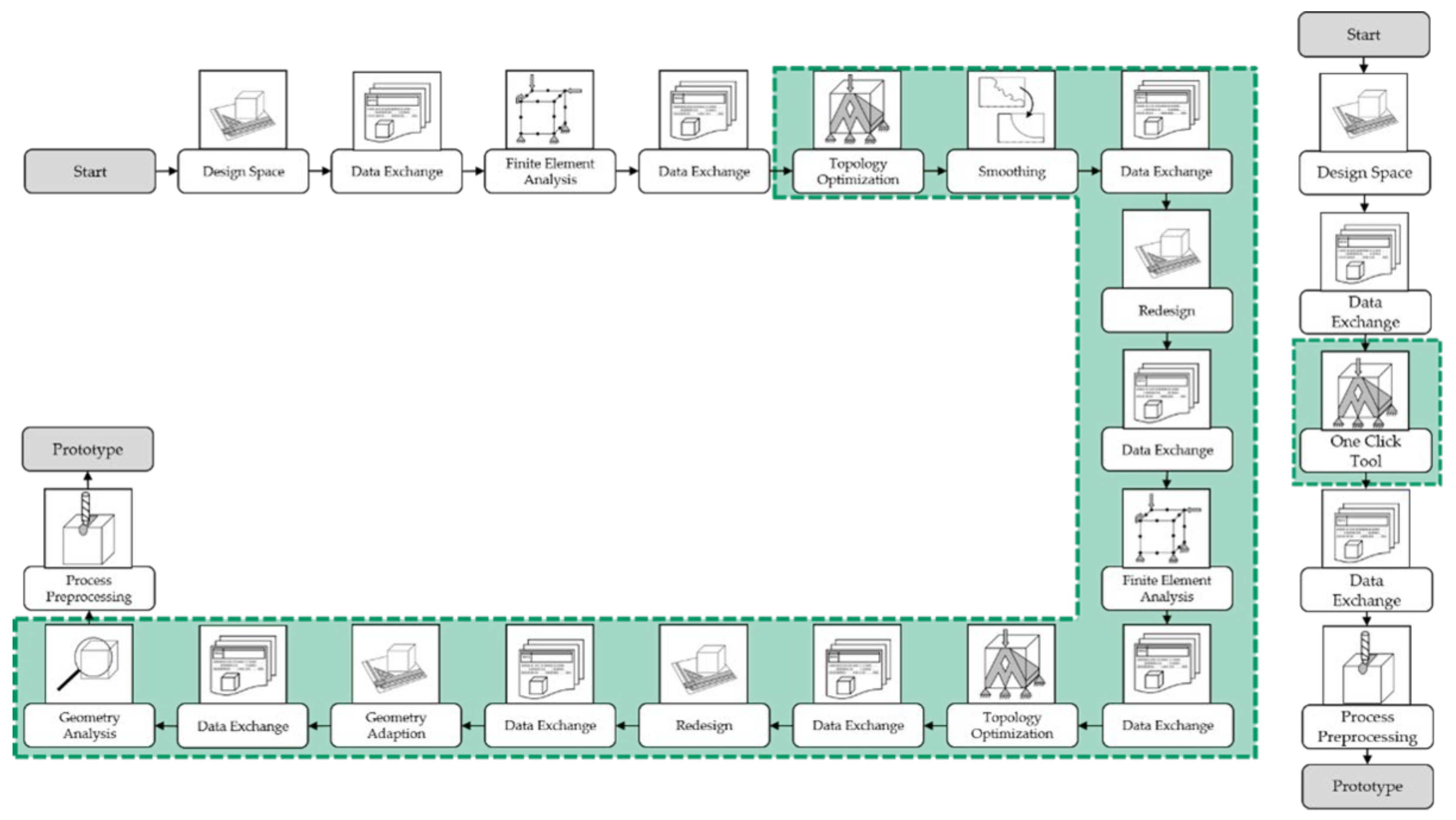
:1. Introduction
2. Materials and Methods
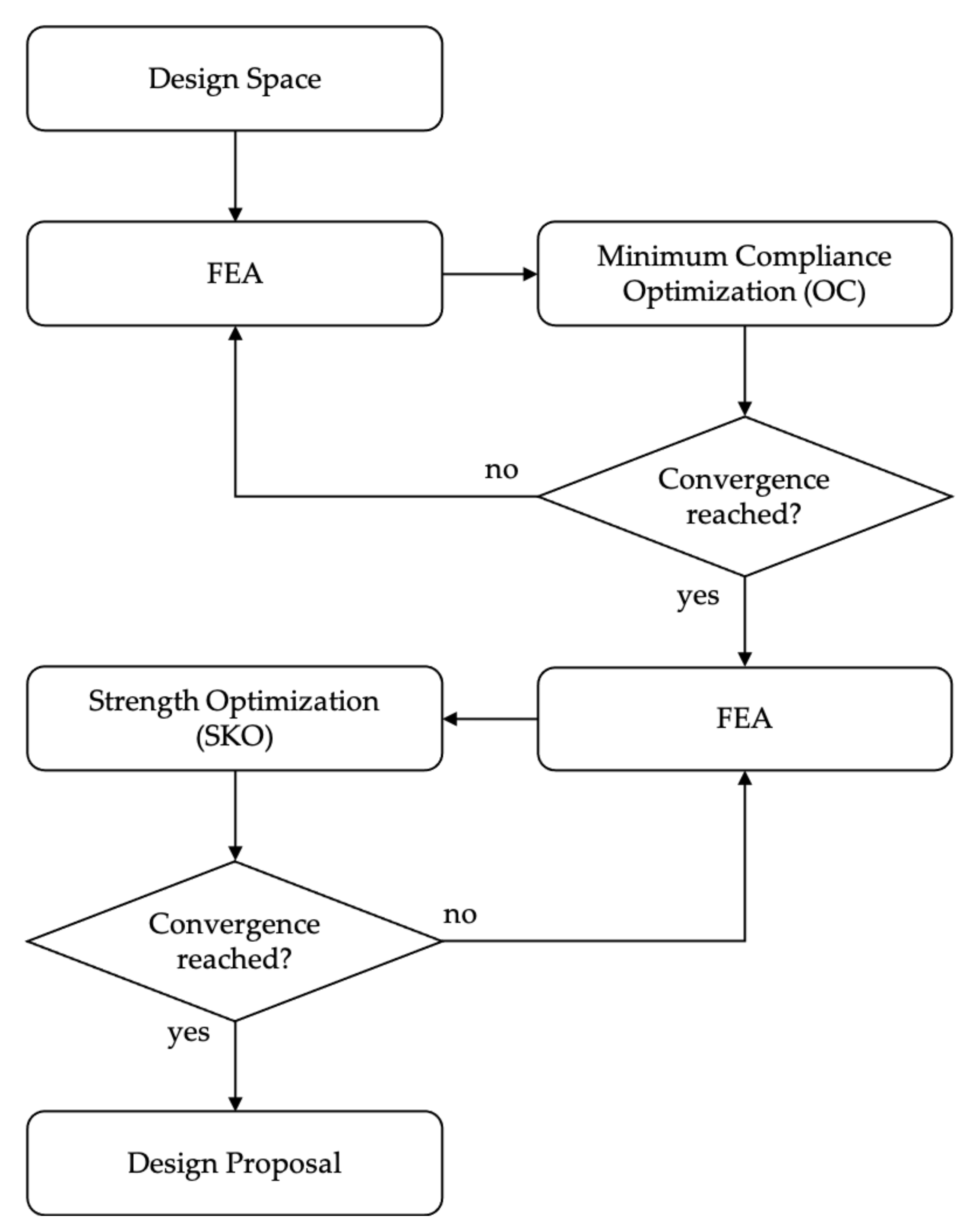
2.1. Topology Optimization for Stiffness and Strength
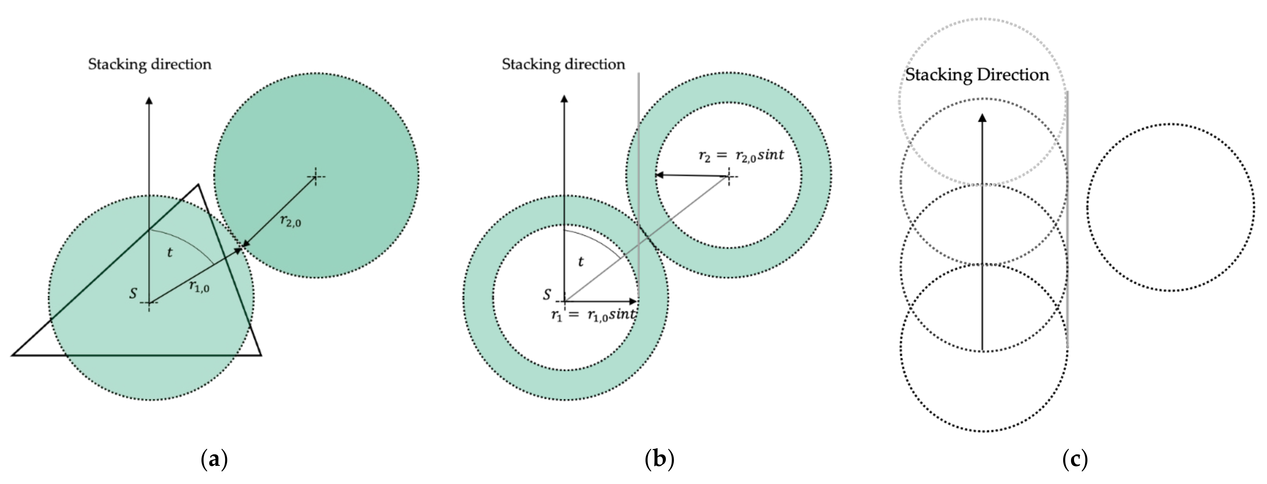
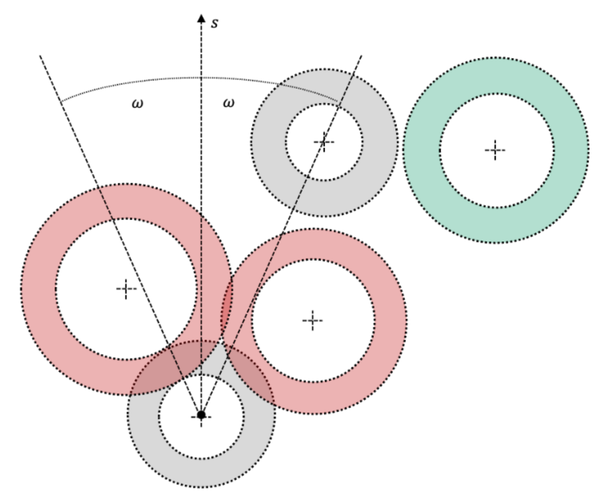
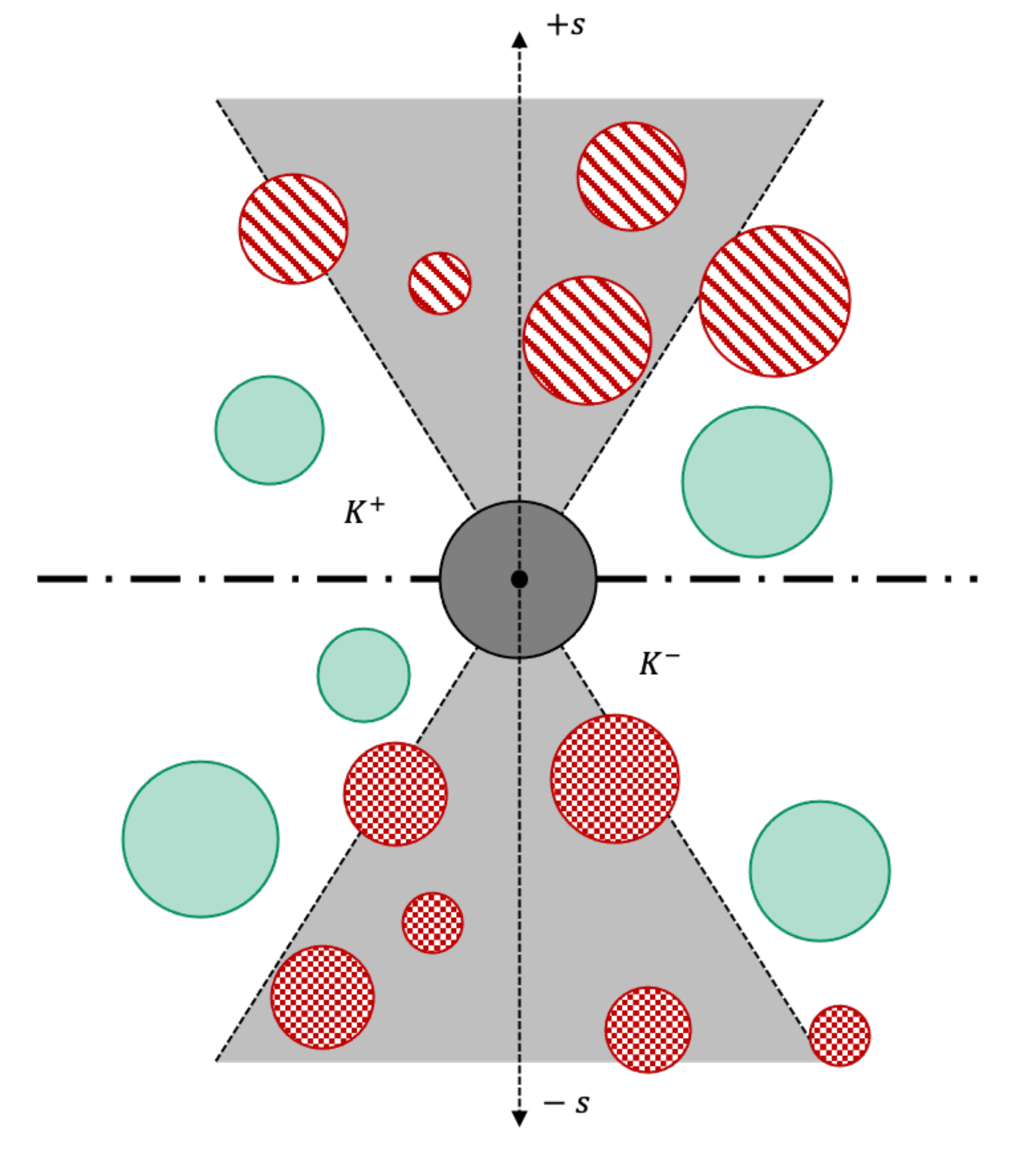
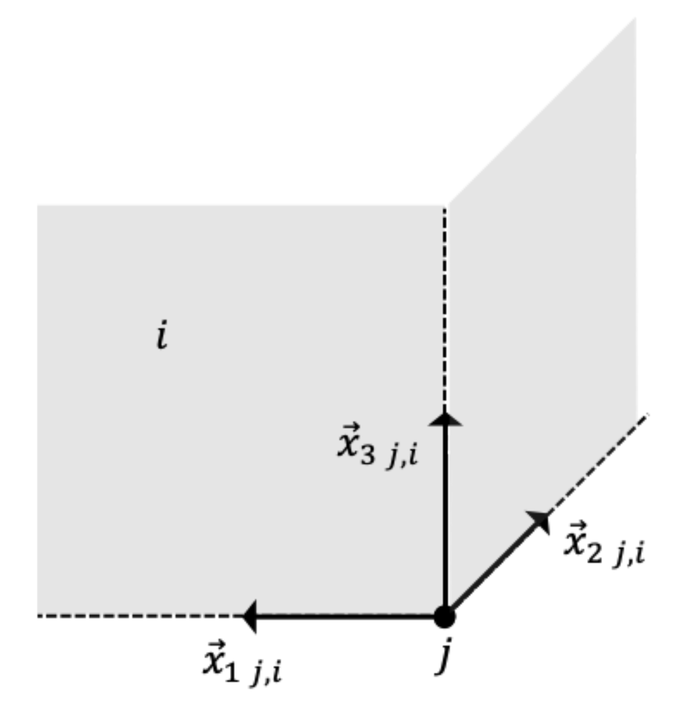
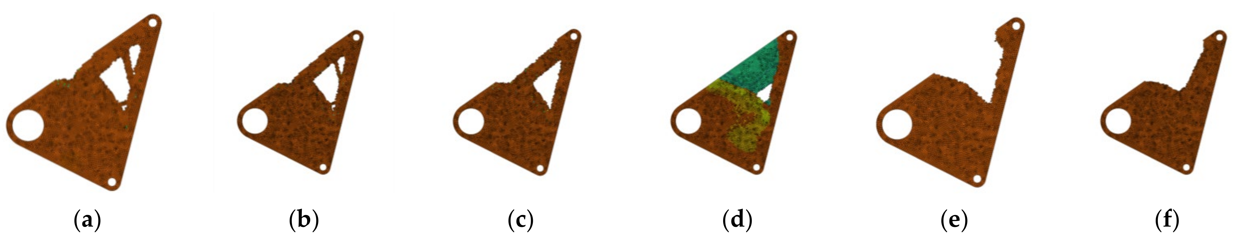
2.2. Finite Spheres as Manufacturing Constraints
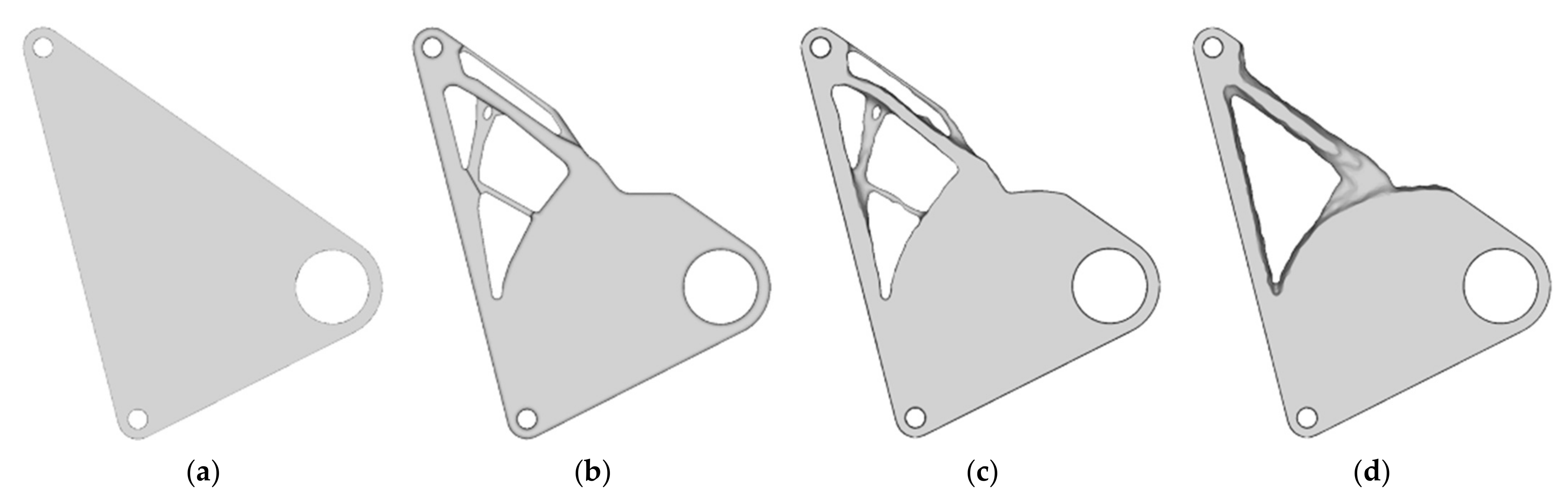
2.3. Two-Step Smoothing
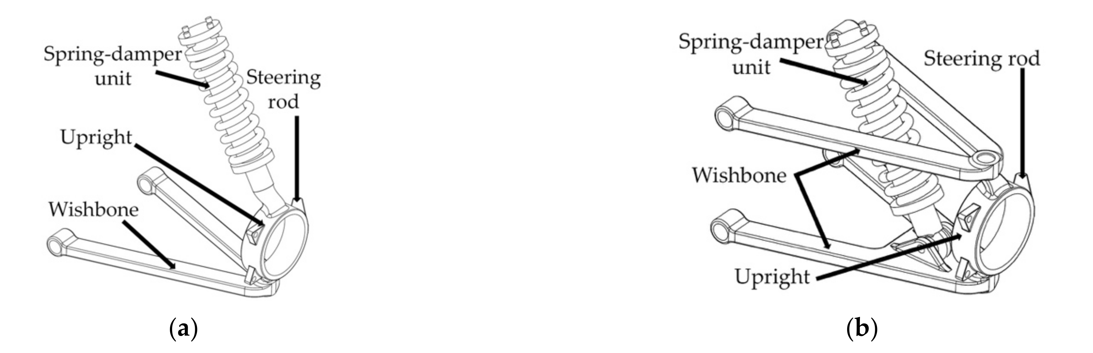
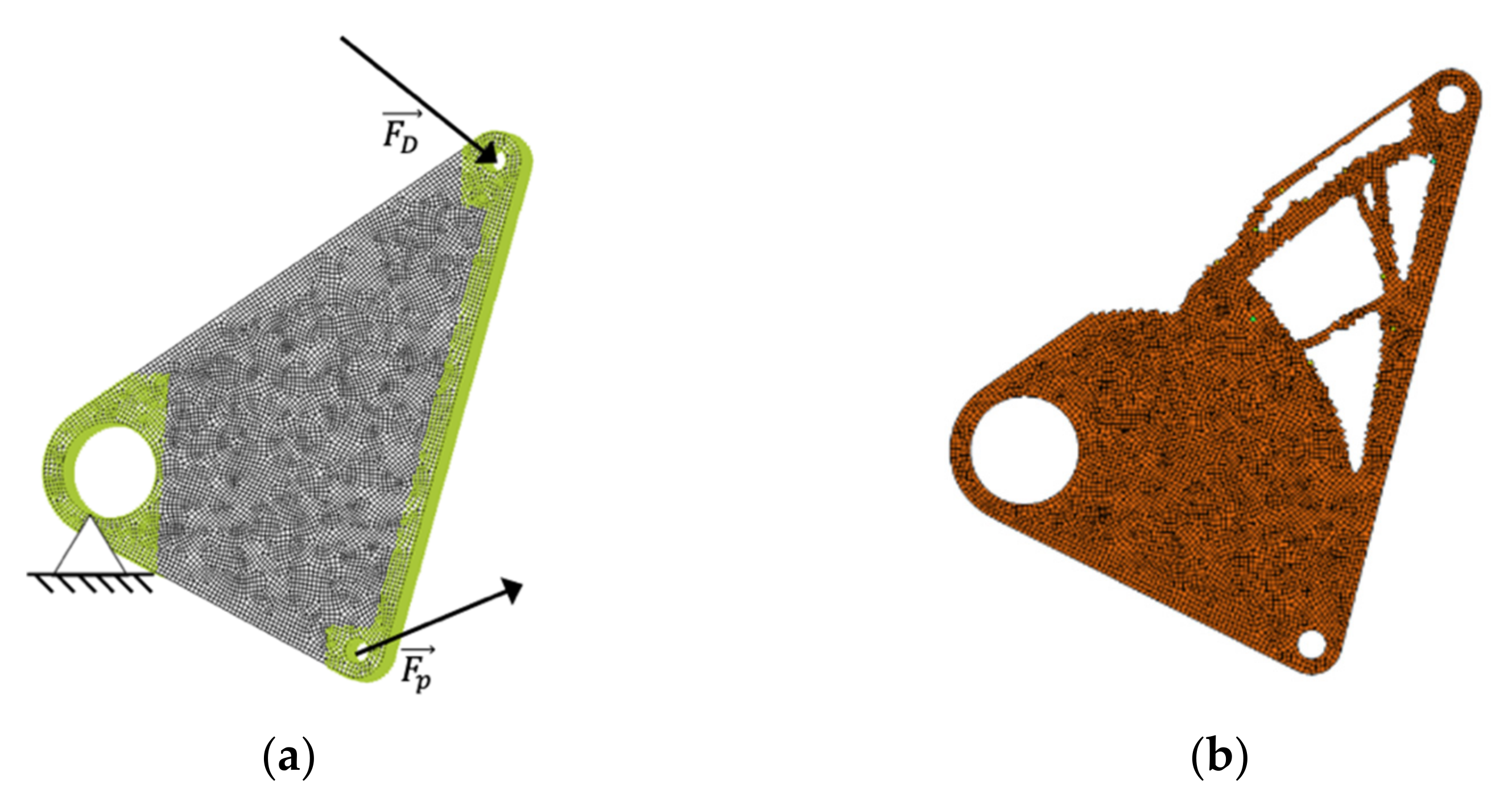
2.4. Example of Application
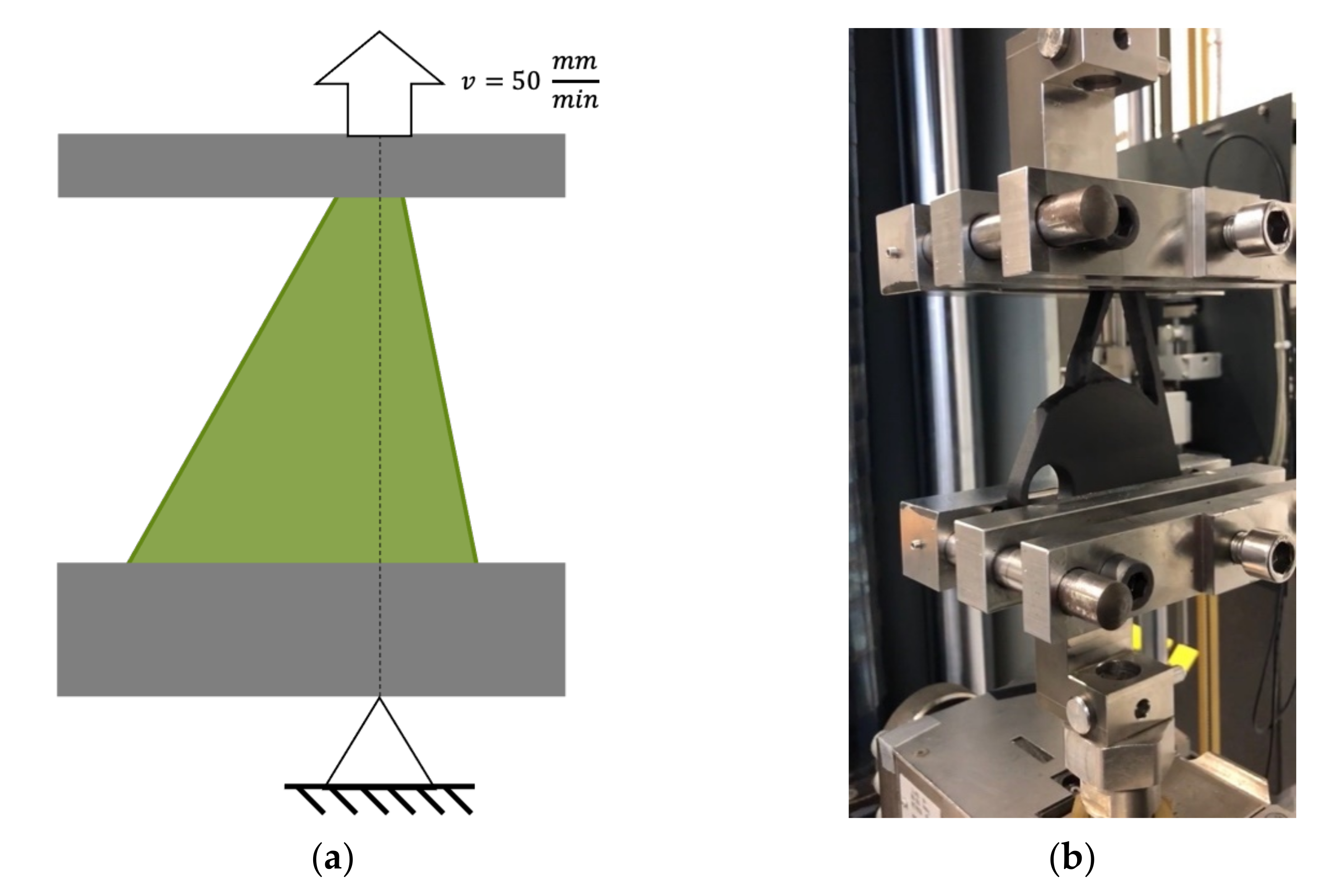
2.5. Testing and Validation
3. Results
3.1. Manufacturability of Design Proposals
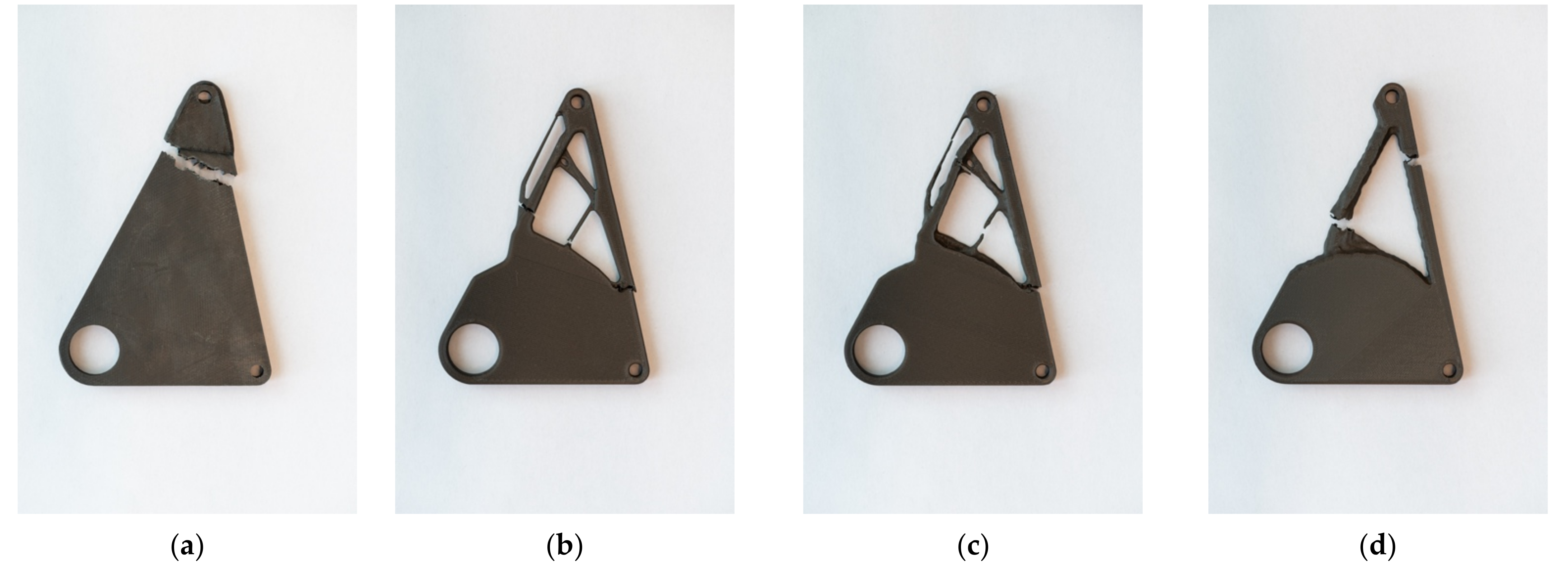
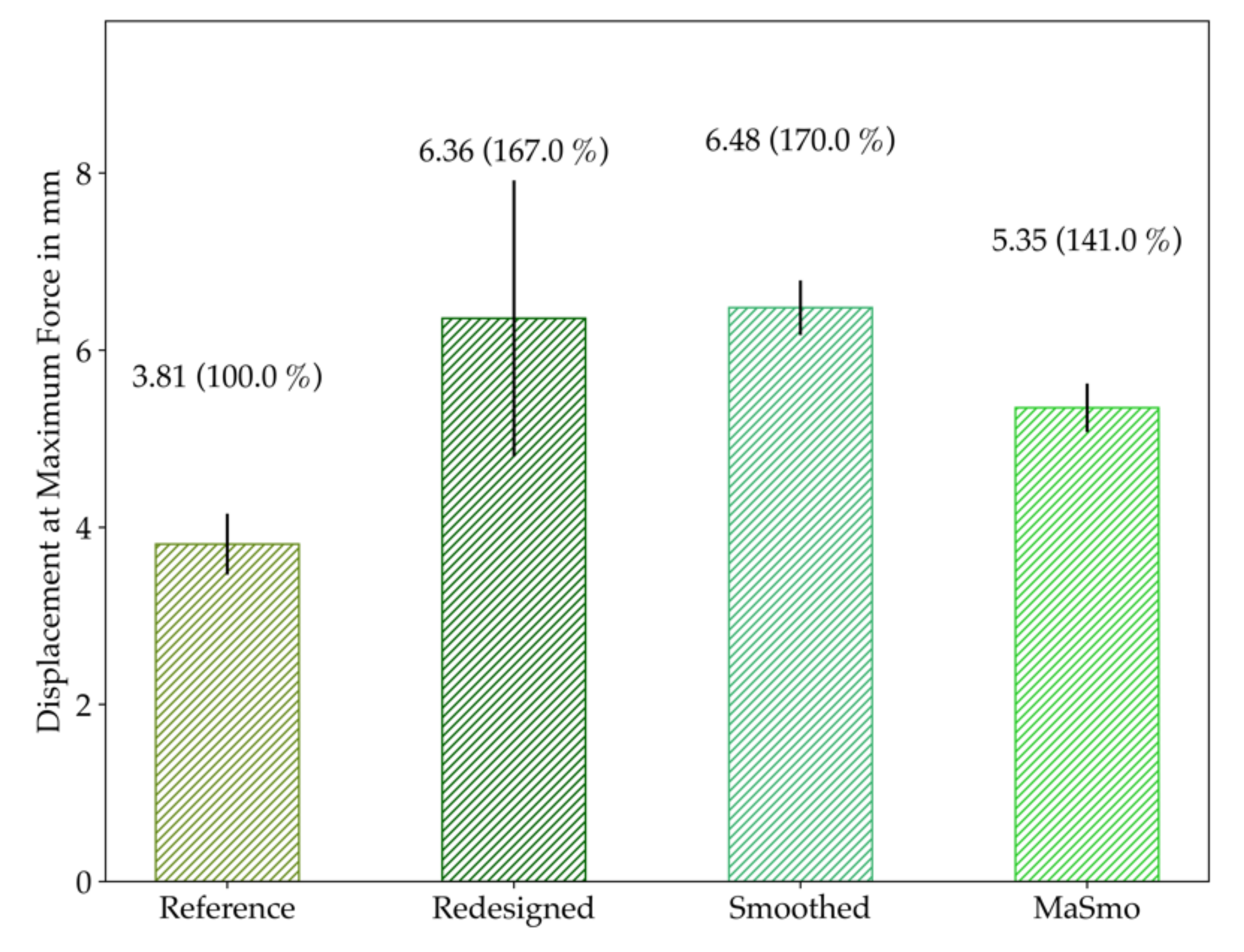
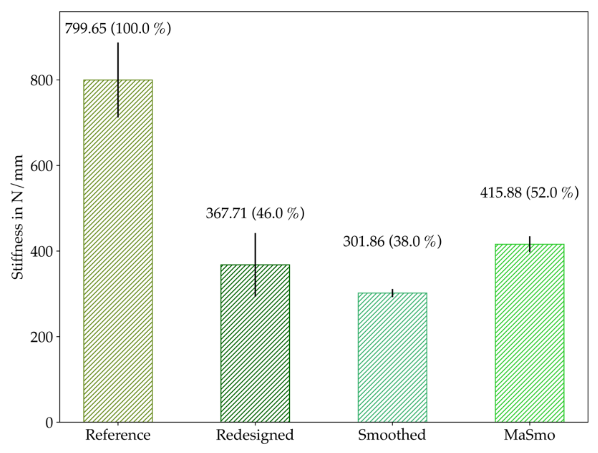
3.2. Experimental Testing
4. Discussion
5. Conclusions
Author Contributions
Funding
Institutional Review Board Statement
Informed Consent Statement
Data Availability Statement
Conflicts of Interest
References
- Glamsch, J.; Deese, K.; Rieg, F. Methods for Increased Efficiency of FEM-Based Topology Optimization. Int. J. Simul. Model. 2019, 18, 453–463. [Google Scholar] [CrossRef]
- Billenstein, D.; Dinkel, C.; Rieg, F. Automated Topological Clustering of Design Proposals in Structural Optimisation. Int. J. Simul. Model. 2018, 17, 657–666. [Google Scholar] [CrossRef]
- Berrocal, L.; Fernández, R.; González, S.; Periñán, A.; Tudela, S.; Vilanova, J.; Rubio, L.; Márquez, J.M.M.; Guerrero, J.; Lasagni, F. Topology optimization and additive manufacturing for aerospace components. Prog. Addit. Manuf. 2018, 4, 83–95. [Google Scholar] [CrossRef]
- Guo, X.; Zhou, J.; Zhang, W.; Du, Z.; Liu, C.; Liu, Y. Self-supporting structure design in additive manufacturing through explicit topology optimization. Comput. Methods Appl. Mech. Eng. 2017, 323, 27–63. [Google Scholar] [CrossRef] [Green Version]
- Zhan, J.; Luo, Y. Robust topology optimization of hinge-free compliant mechanisms with material uncertainties based on a non-probabilistic field model. Front. Mech. Eng. 2019, 14, 201–212. [Google Scholar] [CrossRef]
- Wang, Y.; Kang, Z. Structural shape and topology optimization of cast parts using level set method. Int. J. Numer. Methods Eng. 2017, 111, 1252–1273. [Google Scholar] [CrossRef]
- Tsavdaridis, K.D.; Kingman, J.J.; Toropov, V.V. Application of structural topology optimisation to perforated steel beams. Comput. Struct. 2015, 158, 108–123. [Google Scholar] [CrossRef] [Green Version]
- Lagaros, N.D.; Papadrakakis, M.; Kokossalakis, G. Structural optimization using evolutionary algorithms. Comput. Struct. 2002, 80, 571–589. [Google Scholar] [CrossRef] [Green Version]
- Sigmund, O. On the Design of Compliant Mechanisms Using Topology Optimization*. Mech. Struct. Mach. 1997, 25, 493–524. [Google Scholar] [CrossRef]
- Larsen, U.D.; Signund, O.; Bouwsta, S. Design and fabrication of compliant micromechanisms and structures with negative Poisson’s ratio. J. Microelectromech. Syst. 1997, 6, 99–106. [Google Scholar] [CrossRef] [Green Version]
- Srivastava, S.; Salunkhe, S.; Pande, S.; Kapadiya, B. Topology optimization of steering knuckle structure. Int. J. Simul. Multidiscip. Des. Optim. 2020, 11, 4. [Google Scholar] [CrossRef]
- Ismail, A.Y.; Na, G.; Koo, B. Topology and Response Surface Optimization of a Bicycle Crank Arm with Multiple Load Cases. Appl. Sci. 2020, 10, 2201. [Google Scholar] [CrossRef] [Green Version]
- Shi, G.; Guan, C.; Quan, D.; Wu, D.; Tang, L.; Gao, T. An aerospace bracket designed by thermo-elastic topology optimization and manufactured by additive manufacturing. Chin. J. Aeronaut. 2020, 33, 1252–1259. [Google Scholar] [CrossRef]
- Calabrese, M.; Primo, T.; Del Prete, A. Optimization of Machining Fixture for Aeronautical Thin-walled Components. Procedia CIRP 2017, 60, 32–37. [Google Scholar] [CrossRef]
- Klippstein, H.; Hassanin, H.; Sanchez, A.D.D.C.; Zweiri, Y.; Seneviratne, L. Additive Manufacturing of Porous Structures for Unmanned Aerial Vehicles Applications. Adv. Eng. Mater. 2018, 20, 1800290. [Google Scholar] [CrossRef]
- TopOpt Software and Apps. Available online: https://www.topopt.mek.dtu.dk/apps-and-software (accessed on 1 March 2021).
- Sigmund, O.; Maute, K. Topology optimization approaches. Struct. Multidisc. Optim. 2013, 48, 1031–1055. [Google Scholar] [CrossRef]
- Harzheim, L. Strukturoptimierung Grundlagen und Anwendungen, 3rd ed.; Europa-Lehrmittel: Haan-Gruiten, Germany, 2019. [Google Scholar]
- Chandrasekhar, A.; Suresh, K. TOuNN: Topology Optimization using Neural Networks. Struct. Multidiscip. Optim. 2020, 1–15. [Google Scholar] [CrossRef]
- Clausen, A.; Andreassen, E.; Sigmund, O. Topology optimization of 3D shell structures with porous infill. Acta Mech. Sin. 2017, 33, 778–791. [Google Scholar] [CrossRef] [Green Version]
- Dapogny, C.; Estevez, R.; Faure, A.; Michailidis, G. Shape and topology optimization considering anisotropic features induced by additive manufacturing processes. Comput. Methods Appl. Mech. Eng. 2019, 344, 626–665. [Google Scholar] [CrossRef] [Green Version]
- Liu, S.; Li, Q.; Liu, J.; Chen, W.; Zhang, Y. A Realization Method for Transforming a Topology Optimization Design into Additive Manufacturing Structures. Engineering 2018, 4, 277–285. [Google Scholar] [CrossRef]
- Meng, L.; Zhang, W.; Quan, D.; Shi, G.; Tang, L.; Hou, Y.; Breitkopf, P.; Zhu, J.; Gao, T. From Topology Optimization Design to Additive Manufacturing: Today’s Success and Tomorrow’s Roadmap. Arch. Comput. Methods Eng. 2020, 27, 805–830. [Google Scholar] [CrossRef]
- Plocher, J.; Panesar, A. Review on design and structural optimisation in additive manufacturing: Towards next-generation lightweight structures. Mater. Des. 2019, 183, 108164. [Google Scholar] [CrossRef]
- Strömberg, N. Optimal grading of TPMS-based lattice structures with transversely isotropic elastic bulk properties. Eng. Optim. 2020, 1–13. [Google Scholar] [CrossRef]
- Thompson, M.K.; Moroni, G.; Vaneker, T.; Fadel, G.; Campbell, R.I.; Gibson, I.; Bernard, A.; Schulz, J.; Graf, P.; Ahuja, B.; et al. Design for Additive Manufacturing: Trends, opportunities, considerations, and constraints. CIRP Ann. 2016, 65, 737–760. [Google Scholar] [CrossRef] [Green Version]
- Schmidt, M.-P.; Pedersen, C.B.W.; Gout, C. On structural topology optimization using graded porosity control. Struct. Multidiscip. Optim. 2019, 60, 1437–1453. [Google Scholar] [CrossRef]
- Strömberg, N. Automatic Postprocessing of Topology Optimization Solutions by Using Support Vector Machines. In Proceedings of the ASME 2018 International Design Engineering Technical Conferences & Computers and Information in Engineering Conference IDETC/CIE 2018, Quebec City, QC, Canada, 26–29 August 2018. [Google Scholar] [CrossRef]
- Harzheim, L.; Graf, G. A review of optimization of cast parts using topology optimization. Struct. Multidiscip. Optim. 2005, 30, 491–497. [Google Scholar] [CrossRef]
- Frisch, M.; Dörnhöfer, A.; Nützel, F.; Rieg, F. Fertigungsrestriktionen in der Topologieoptimierung. In Integrierte Produktentwicklung für Einen Globalen Markt, Proceedings of the 9. Gemeinsames Kolloquium Konstruktionstechnik, Aachen, Germany, 6–7 October 2011; Brökel, K., Grote, K.-H., Rieg, F., Stelzer, R., Eds.; Shaker: Aachen, Germany, 2011. [Google Scholar]
- Vatanabe, S.L.; Lippi, T.N.; De Lima, C.R.; Paulino, G.H.; Silva, E.C. Topology optimization with manufacturing constraints: A unified projection-based approach. Adv. Eng. Softw. 2016, 100, 97–112. [Google Scholar] [CrossRef] [Green Version]
- Harzheim, L.; Graf, G. A review of optimization of cast parts using topology optimization II–Topology optimization with manufacturing constraints. Struct. Multidiscip. Optim. 2005, 31, 388–399. [Google Scholar] [CrossRef]
- Franke, T.; Fiebig, S.; Bartz, R.; Vietor, T.; Hage, J.; Hofe, A.V. Adaptive Topology and Shape Optimization with Integrated Casting Simulation. In EngOpt 2018 Proceedings of the 6th International Conference on Engineering Optimization, 2018; Rodrigues, H.C., Herskovits, J., Mota Soares, C.M., Araujo, A.L., Guedes, J.M., Folgado, J.O., Moleiro, F., Madeira, J.F.A., Eds.; Springer International Publishing: Cham, Switzerland, 2018. [Google Scholar] [CrossRef]
- Franke, T.; Fiebig, S.; Paul, K.; Vietor, T.; Sellschopp, J. Topology Optimization with Integrated Casting Simulation and Parallel Manufacturing Process Improvement. In Advances in Structural and Multidisciplinary Optimization, Proceedings of the World Congress of Structural and Multidisciplinary Optimisation, Braunschweig, Germany, 5–9 June 2017; Schumacher, A., Vietor, T., Fiebig, S., Bletzinger, K.U., Maute, K., Eds.; Springer International Publishing: Cham, Switerland, 2018. [Google Scholar] [CrossRef]
- Mirzendehdel, A.M.; Suresh, K. Support structure constrained topology optimization for additive manufacturing. Comput. Des. 2016, 81, 1–13. [Google Scholar] [CrossRef] [Green Version]
- Gaynor, A.T.; Guest, J.K. Topology optimization considering overhang constraints: Eliminating sacrificial support material in additive manufacturing through design. Struct. Multidiscip. Optim. 2016, 54, 1157–1172. [Google Scholar] [CrossRef]
- Kandemir, V.; Dogan, O.; Yaman, U. Topology optimization of 2.5D parts using the SIMP method with a variable thickness approach. In Proceedings of the 28th International Conference on Flexible Automation and Intelligent Manufacturing (FAIM2018), Columbus, OH, USA, 11–14 June 2018. Procedia Manufacturing. [Google Scholar] [CrossRef]
- Leary, M.; Merli, L.; Torti, F.; Mazur, M.; Brandt, M. Optimal topology for additive manufacture: A method for enabling additive manufacture of support-free optimal structures. Mater. Des. 2014, 63, 678–690. [Google Scholar] [CrossRef]
- Saadlaoui, Y.; Milan, J.-L.; Rossi, J.-M.; Chabrand, P. Topology optimization and additive manufacturing: Comparison of conception methods using industrial codes. J. Manuf. Syst. 2017, 43, 178–186. [Google Scholar] [CrossRef]
- Frisch, M. Entwicklung eines Hybridalgorithmus zur Steifigkeits- und Spannungsoptimierten Auslegung von Konstruktionselementen. Ph.D. Thesis, Univeristy of Bayreuth, Bayreuth, Germany, 2015. [Google Scholar]
- Deese, K.; Geilen, M.; Rieg, F. A Two-Step Smoothing Algorithm for an Automated Product Development Process. Int. J. Simul. Model. 2018, 17, 308–317. [Google Scholar] [CrossRef]
- Rosnitschek, T.; Siegel, T.; Linke, D.; Mailänder, P.; Kamp, D.; Rieg, F. Optimizing material exploitation in the direct additive manufacturing of topology-optimized structures. In Nachhaltige Produktentwicklung, Proceedings of the 18. Gemeinsames Kolloquium Konstruktionstechnik, Duisburg, Germany, 1–2 October 2020; Corves, B., Gericke, K., Grote, K.-H., Lohrengel, A., Löwer, M., Nagarajah, A., Rieg, F., Scharr, G., Stelzer, R., Eds.; University of Duisburg-Essen: Duisburg, Germany, 2020. [Google Scholar] [CrossRef]
- Z88. Available online: https://z88.de (accessed on 10 February 2021).
- Baumgartner, A.; Harzheim, L.; Mattheck, C. SKO (soft kill option): The biological way to find an optimum structure topology. Int. J. Fatigue 1992, 14, 387–393. [Google Scholar] [CrossRef]
- Ersoy, M.; Gies, S. Fahrwerkhandbuch; Springer International Publishing: Berlin/Heidelberg, Germany, 2017. [Google Scholar]
- Trzesniowski, M. (Ed.) Fahrwerk. In Handbuch Rennwagentechnik, 2nd ed.; Springer-Vieweg: Wiesbaden, Germany, 2019; Volume 4. [Google Scholar]
- Elefant Racing Bayreuth. Available online: https://elefantracing.de (accessed on 26 February 2021).
- Markforged Onyx Material Data. Available online: https://markforged.com/materials/plastics/onyx (accessed on 10 February 2021).
- Pedregosa, F.; Varoquaux, G.; Gramfort, A.; Michel, V.; Thirion, B.; Grisel, O.; Blondel, M.; Prettenhofer, P.; Weiss, R.; Du-bourg, V.; et al. Scikit-learn: Machine Learning in Python. JMLR 2011, 85, 2825–2830. [Google Scholar]


| Force Component | Value in N |
|---|---|
| 455 | |
| −750 | |
| 2960 | |
| 2770 |
| Configuration | Algorithm | Manufacturing Constraints | Target Volume | Real Volume | Iterations |
|---|---|---|---|---|---|
| Reference | -- | -- | 100% | 100% | -- |
| Redesigned | TOSS | no | 75% | 77.2% | 100 |
| Smoothed | TOSS | no | 75% | 74.6% | 100 |
| MaSmo | TOSS | Yes | 75% | 75.6% | 41 |
| Feature | Value |
|---|---|
| Manufacturing direction | z axis |
| Manufacturing rate | 0.7 |
| Manufacturing angle | 45 deg. |
| Configuration | Print Time | Plastic Volume | Support Volume | Support Volume Ratio |
|---|---|---|---|---|
| Reference | 100% | 100% | -- | -- |
| Redesigned | 103.2% | 92.0% | 100% | 0.76% |
| Smoothed | 104.3% | 90.0% | 131.6% | 1.03% |
| MaSmo | 95.3% | 88.9% | 52.6% | 0.42% |
Publisher’s Note: MDPI stays neutral with regard to jurisdictional claims in published maps and institutional affiliations. |
© 2021 by the authors. Licensee MDPI, Basel, Switzerland. This article is an open access article distributed under the terms and conditions of the Creative Commons Attribution (CC BY) license (http://creativecommons.org/licenses/by/4.0/).
Share and Cite
Rosnitschek, T.; Hentschel, R.; Siegel, T.; Kleinschrodt, C.; Zimmermann, M.; Alber-Laukant, B.; Rieg, F. Optimized One-Click Development for Topology-Optimized Structures. Appl. Sci. 2021, 11, 2400. https://0-doi-org.brum.beds.ac.uk/10.3390/app11052400
Rosnitschek T, Hentschel R, Siegel T, Kleinschrodt C, Zimmermann M, Alber-Laukant B, Rieg F. Optimized One-Click Development for Topology-Optimized Structures. Applied Sciences. 2021; 11(5):2400. https://0-doi-org.brum.beds.ac.uk/10.3390/app11052400
Chicago/Turabian StyleRosnitschek, Tobias, Rick Hentschel, Tobias Siegel, Claudia Kleinschrodt, Markus Zimmermann, Bettina Alber-Laukant, and Frank Rieg. 2021. "Optimized One-Click Development for Topology-Optimized Structures" Applied Sciences 11, no. 5: 2400. https://0-doi-org.brum.beds.ac.uk/10.3390/app11052400