A Layered KNN-SVM Approach to Predict Missing Values of Functional Requirements in Product Customization

Abstract

The conversion from functional requirements (FRs) to design parameters is the foundation of product customization. However, original customer needs usually result in incomplete FRs, limited by customers’ incomprehension on the design requirements of these products. As the incomplete FRs may undermine the design activities afterwards, managers need to develop an effective approach to predict the missing values of the FR. This study proposes an integrative approach to obtain the complete FR. The k nearest neighbor (KNN) algorithm is employed to predict the missing continuous variables in FR, using the improved distance formula for two incomplete FRs. Support vector machine (SVM) classifiers are adopted to classify the missing categorical variables in FR, combined with directed acyclic graph for multi-class classification. KNN and SVM are then integrated into a multi-layer framework to predict the missing values of FR, where categorical and continuous variables both exist. A case study on the elevator customization is conducted to verify that KNN-SVM is feasible in accurate prediction of elevator FR values. Furthermore, KNN-SVM outperforms other five single and five composite methods, with average reduction in root mean squared error (RMSE) of 39% and 21% against KNN and KNN-Tree, respectively.

1. Introduction

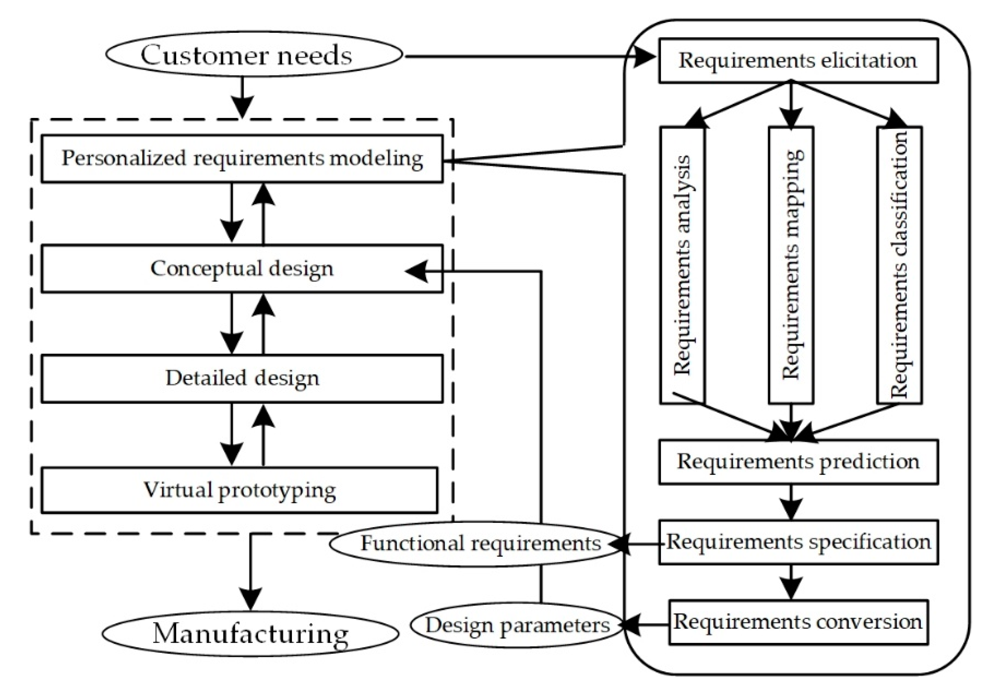
Nowadays, more than half of the industrial products are related to customization [1]. How to satisfy personalized customer needs (CNs) and how to efficiently design the customized products have been the important characteristics to evaluate manufacturing enterprises’ viability and competitiveness. There are four critical stages in product customized design [2]: personalized requirements modeling [3], conceptual design [4], detailed design (i.e., configuration in mass customization [5]), and virtual prototyping (including virtual experience [6] and simulation [7]), as shown in Figure 1. The first stage in the design process—personalized requirements modeling—is the foundation of product customization, including elicitation, analysis, mapping, classification, prediction, specification, and conversion. The process of requirements modeling is to transform CNs into functional requirements (FRs) and FRs into design parameters (DPs), where FR is the intermediate link [8]. FRs and DPs are then input into the design activities afterwards. If there is an error in FR, all the design activities in customization will be susceptible to a domino effect of defaults, which could undermine the final design schemes, lower customers’ satisfaction in experience, and cause redesign. Thus, focusing on the requirements modeling and dealing with the potential problems are imperative to product customized design.

After investigating CNs of different industrial customized products in different communities and numbers of small and medium enterprises, it is obvious that most customers cannot put forward specific and complete requirements to match the design requirements of products. Thus, FR transformed by CN usually contains missing values, which may affect the conversion from FR to DP. Subjective CN is easy to propose, such as appearance requirements in customized clothing [9]. Other quality requirements, which impose constraints on the design or implementation (such as performance requirements, security, or reliability) [10,11], are too professional for customers to put forward. Some customers may leave some questions about requirement questionnaires consciously or unconsciously. In addition, developing product customization systems is popular in many manufacture sectors. However, the missing values of requirements or other aspects, caused by information gap, measurement error, and equipment failure, are neglected. On the other hand, each order is personalized in customization, where missing values prediction for each FR needs to be personalized. Missing values in FR is a potential problem to be addressed in requirements modeling of product customized design, which is the key motivation of this paper.

In this context, a number of researches have been conducted to predict the missing personalized requirements, as detailed in Section 2.1. From a review of existing literature, this research is helpful to collect more correct CN, which is also helpful to transform CN into the more complete FR afterwards. However, this research is focused on predicting CN instead of FR [12,13,14,15]. Many implicit CNs are still subjective requirements rather than quality requirements [16,17,18], which results in FR still bei incomplete in parts of performance requirements, structure requirements, or other design requirements. Starting with incomplete FRs directly, this study aims to introduce an approach to predict the missing values of FR. The principle objectives of this study are:

• Explore the interconnections among different orders from customers to predict the missing values of FR.
• Determine the optimal predicted values with a feasible framework and algorithms for missing values prediction of FR.

This study proposes an integrative approach to predict the missing values of FR in product customization. By analyzing the attributes and values of FR in industrial customized products, FR can be divided into continuous and categorical variables. Missing values in different attributes are predicted by different methods. Thus, a multi-layer framework is proposed, where the k nearest neighbor (KNN) algorithm and support vector machine (SVM) classifier are adopted to predict the missing continuous and categorical variables in FR, respectively. A case study on the elevator customization is conducted to verify the proposed approach. KNN-SVM is compared with five single methods (KNN, GRNN, SVD, BPCA, and BBPCA) and five composite methods (KNN-GRNN, KNN-SVD, KNN-BBPCA, KNN-Bay, and KNN-Tree), with average reduction in root mean squared error (RMSE) of 39% and 21% against KNN and KNN-Tree, respectively. The computation time of the proposed approach is always less than two seconds. The proposed approach is helpful for managers to accurately predict the missing values in FR, is beneficial to obtain the complete requirements in design process, and can improve product design efficiency.

This paper is structured as follows. Section 2 reviews the related work in requirements prediction and missing values imputation. Section 3 presents the problem description and framework formulation for missing values prediction. Following that, Section 4 details the proposed prediction approach, which integrates KNN and SVM into a multi-layer framework. A case study on the elevator customization is conducted in Section 5. Concluding remarks and future work in Section 6 end the paper.

2. Literature Review

2.1. Requirements Prediction in Product Customized Design

Personalized requirements modeling is the foundation of product customized design. Missing requirements prediction is a potential problem in requirements modeling, gaining the ever-increasing attention of researchers. Many studies have been conducted on this topic, including predicting the implicit requirements and forecasting the trends of requirements.

One research field is implicit requirements prediction. With the development of the Internet and Internet of Things (IoT), many researches extract implicit CN online or by a cloud-service platform combined with some new techniques in data mining. Guo et al. [12] tried to extract and normalize the implicit requirements by a series of techniques including metaphor, clustering, mapping, and visualization; the requisite requirements collected and predicted for product customization are neglected. Qi et al. [13] designed an automatic filtering model integrated with the Kano model to analyse online reviews, and the mined information is applied to improve product design strategies. Yan et al. [14] built a consumer-centric relationship network by IoT technologies to predict the personalized requirements. Jiang et al. [15] analyzed the online reviews by association rule mining based on multi-objective particle swarm optimization for affective design. Zhou et al. [16] proposed a two-layer model for latent CN elicitation through use case reasoning, where SVM is used for sentiment analysis in the first layer, and case analogical reasoning is applied to identify implicit CN characteristics in the second layer. The other research field of requirements prediction concerns requirement status. Song et al. [17] integrated grey theory for fewer requirements data, the Kano model for requirements classification, and a Markov chain for local fluctuations to predict the dynamic requirements. Raharjo et al. [18] estimated and transmitted weights in quality function deployment to the design attributes to deal with dynamics of CN. Min et al. [19] combined theKano model and online reviews to analyze dynamic requirements change in CN.

Many research studies have made full use of online reviews or big data for prediction, which is inspirational. It is useful to link customer groups with clusters of requirements to predict the missing values. However, there exist some technical challenges in requirements prediction. First, most predicted results are indirect and need analysis and processing by professional managers. Then, most approaches focus mainly on the subjective requirements, which is incomplete in real-world requirements for product customization. Finally, CN is often regarded as an individual object, without considering the design activities afterwards. To bridge this gap, this paper presents an approach for predicting missing values of FR, considering the characteristics of different requirements and providing valuable predicted results.

2.2. Imputation Approaches for Missing Values

Traditional missing values prediction methods in FR rely on managers’ experience, investigation, and communications with customers, which are popular in mass production. In smart customization, intelligent methods should be proposed to solve this problem for a lot of personalized orders. Missing values imputation is a hotspot issue in data mining and machine learning nowadays. Requirements prediction in product customized design can learn from this research. We conclude the main methods of missing values imputation in

Table 1. Missing values imputation methods.

Category	Model/Methodology	Continuous Variables	Categorical Variables	Application
Rule-based	Imputation with master data and a class of editing rules [20]	√		Two real-word datasets
	Five strategies used for different attributes [21]	√	√	Preterm birth datasets
Statistics-based	Estimation of mean values and covariance matrices [22]	√		Surface temperature data
	Expectation maximization with bootstrapping [23]	√	√	Amelia II (software)
Model-based	Gray KNN [24]	√	√	Six real-world datasets
	Sequential KNN [25]	√		DNA microarray analysis
	Generalized regression neural network (GRNN) [26]		√	30 synthetic datasets + 67 public datasets + one new real-world dataset
	Bayesian principal component analysis (BPCA) [27]	√		Gene expression profile data
	Bicluster-based BPCA [28]	√		DNA microarray analysis
	Random forest [29]	√	√	Four datasets for continuous, three datasets for categorical, and three datasets for mixed variables
	Singular value decomposition (SVD) with KNN [30]	√		DNA microarray analysis
	Kernel density clustering combined with decision tree [31]		√	Eight real-world datasets
	Formal optimization framework with KNN, SVM, and decision trees [32]	√	√	84 real-word datasets
Human–computer interaction	Crowdsourcing optimized by knowledge base [33]	√	√	Two real-world datasets
	Crowdsourcing with Bayesian network [34]	√		Two real-world datasets

for reference.

Data in missing values imputation are divided into continuous and categorical variables, which are adoptable to predict missing values of FR. However, there are a few methods considering continuous and categorical variables synchronously. To improve the accuracy of predicted values, it is necessary to propose and integrate different imputation methods for different characteristics of requirements. Model-based methods for missing values imputation outperform other methods, which seem appropriate to the problem at hand. In addition, the applications of these methods focus mostly on the public datasets. To the best of authors’ knowledge, there are few research studies on the missing values prediction in FR. Existing methods need to be improved for practical applications in product customized design.

3. Multi-Layer Framework for Missing Values Prediction

3.1. Problem Description

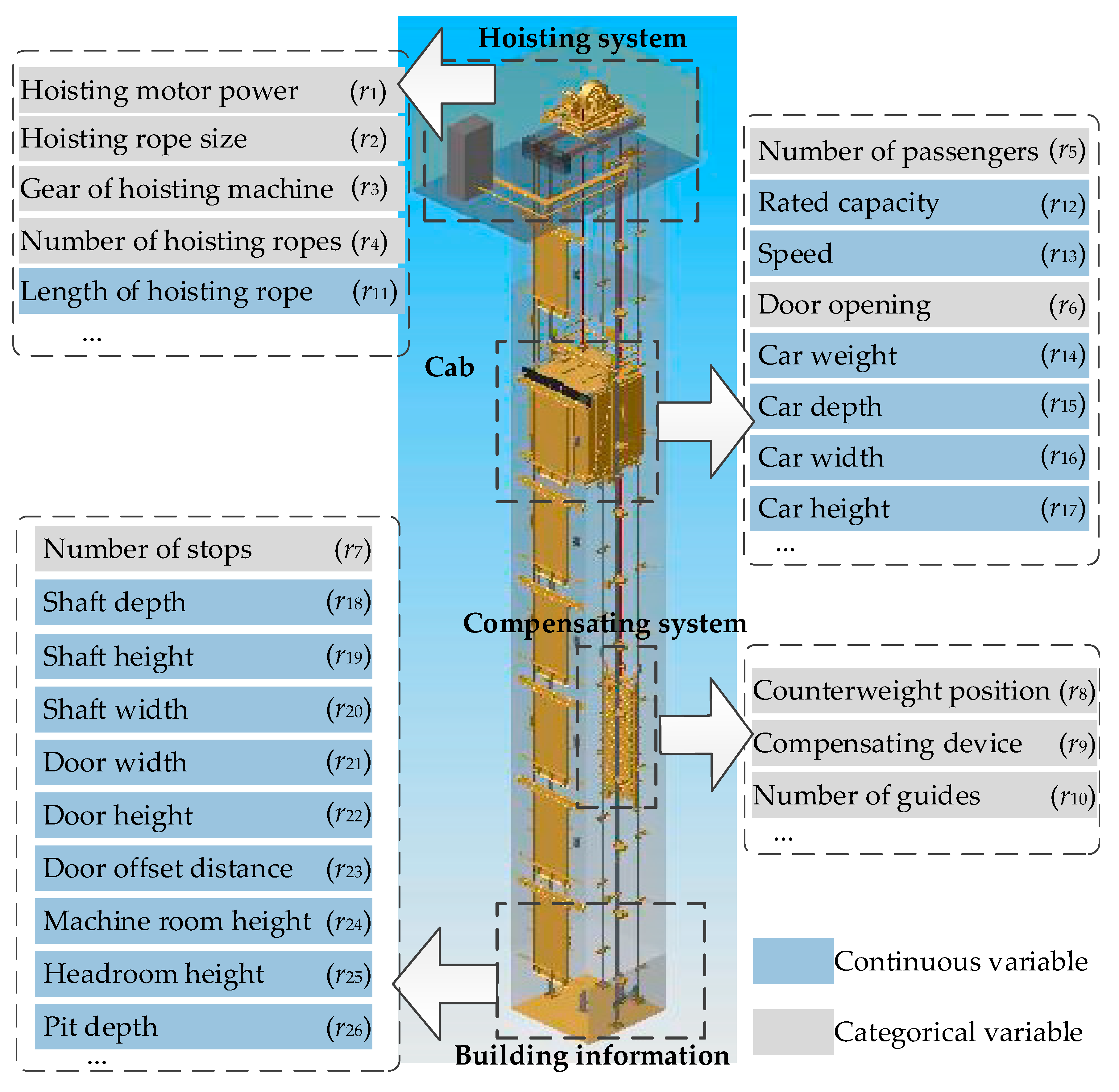
This study addresses the problem about the missing value prediction in FR for product customized design. We take customized elevators as an example to describe this problem. Elevators, as a classic industrial product, are customized in each building. We present FR of a real-word elevator product in Figure 2. Managers need complete FR to be transformed into DP for the design activities afterwards.

For the personalized CN, many elevator manufacturing enterprises have developed the requirements management system online. Otis Elevator Company in Yonkers, NY, USA, has developed Architect’s Assistant™ (http://aa.otis.com/aa/cda/cdalogin.aspx) (Accessed on 2 March 2021) and CabCreat™ (http://cabcreate.otis.com/) (Accessed on 2 March 2021) for requirements elicitation online. Hitachi Company in Tokyo, Japan, developed the smartDecorator software for customized elevator decoration. However, FR transformed from the obtained CN is mostly incomplete in these systems. For example, FR in the hoisting system of elevator (i.e., r₁–r₄ and r₁₁ in Figure 2) cannot be directly obtained or transformed from CN in Architect’s Assistant™, because these requirements are too professional for customers to put forward. In addition, incorrect FR could impact the final design schemes. For example, with the larger predicted value of hoisting motor power (r₁) compared with the ground truth in FR, the following negative situations may happen: (1) the increase in the price of elevator may lower customers’ satisfaction; (2) there exists more energy cost and it is not conducive to clean production; (3) long-time operation in low power may shorten the service life and increase maintenance costs.

FR can be expressed as x with p values, where the number of categorical and continuous variables are p₀ ($j\in \{1,2,\dots ,p_0\}$) and p₁ ($j\in \{p_0+1,p_0+2,\dots ,p_0+p_1\}$), respectively, $p=p_0+p_1$. Then, FR matrix X is composed of N pieces of x, $\mathit{X}={\left\{{\mathit{x}}_i\right\}}_{i=1}^N$. Incomplete FR matrix with missing values is denoted as X^miss. The coordinates of missing values are

$$M_0=\{(i,j):1\le i\le N,1\le j\le p_0,x_{ij}\mathrm{is}\mathrm{missing}\},$$

(1)

$$M_1=\{(i,j):1\le i\le N,p_0+1\le j\le p,x_{ij}\mathrm{is}\mathrm{missing}\}.$$

(2)

We aim to predict the missing values with only X^miss by mining the interconnections among different x and provide the valuable predicted results to managers.

3.2. Framework Formulation

There are two data types, categorical and continuous variables, in FR. Traditional imputation methods handle only the continuous variables [27,28,30]. They transfer the categorical variables into continuous variables before imputation. Then, the predicted categorical variables are mapped into labels. The errors in this process are unavoidable. More advanced methods are proposed to divide these two data types [24,29,32]. We found that categorical variables in FR are more important than the continuous ones. Customers prefer to choose rather than fill in the blanks when proposing CN, and the predicted results of categorical variables are easier to be judged by managers.

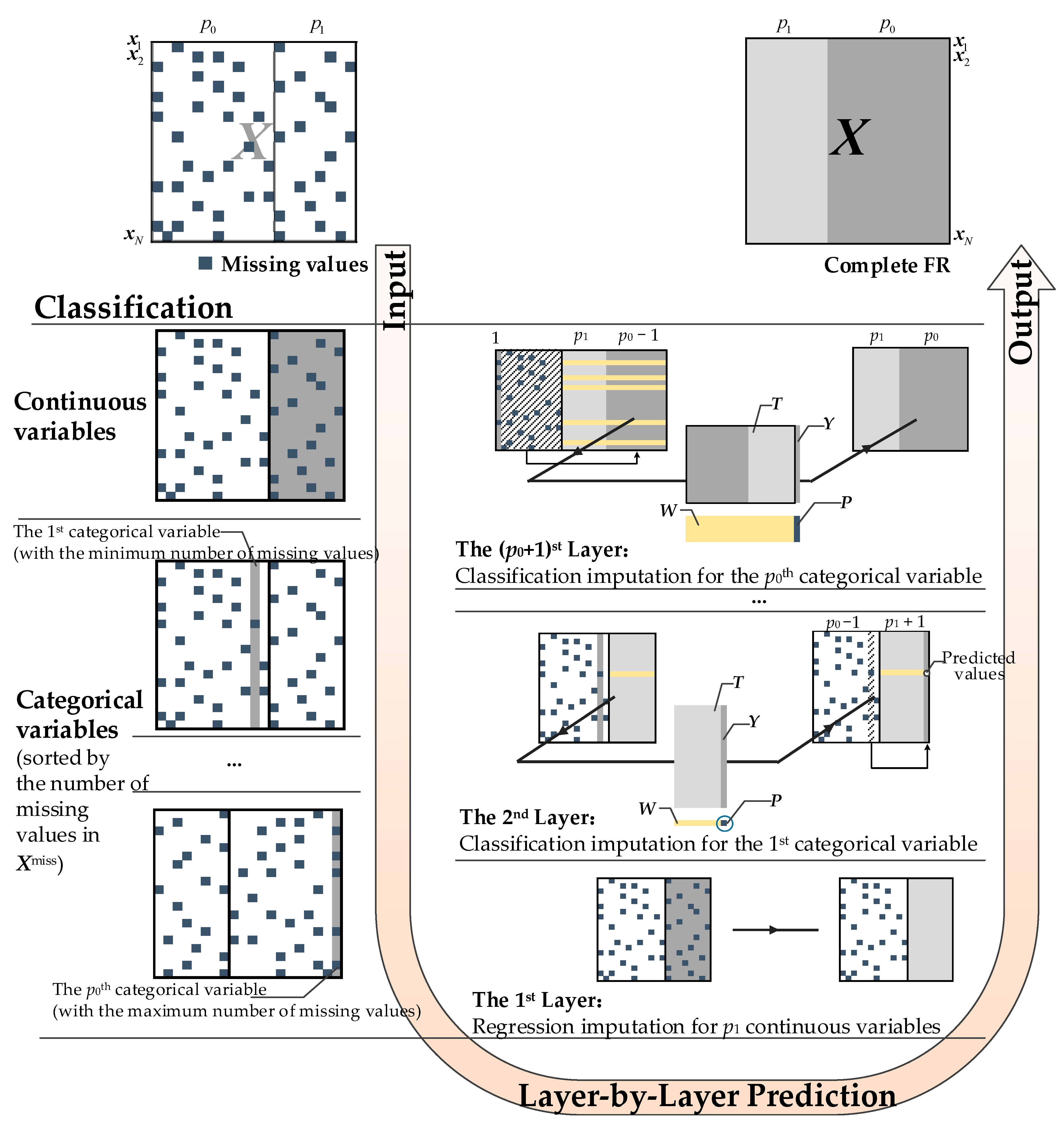
A multi-layer framework is presented in Figure 3. After classifying different data types in X^miss, the complete X can be obtained by layer-by-layer prediction with two different imputation methods. The 1st layer is used for predicting missing continuous variables. We can choose one regression imputation method in the first layer. Then, the 2nd to the (p₀ + 1)th layers in the framework are used for predicting categorical variables. For example, in the second layer, we have p₁ continuous variables with complete values in X, denoted as ${\mathit{X}}_2^{\mathrm{mis}\mathrm{s}}$, and the missing values of the first categorical variable will be predicted. The first categorical variable is defined as the ath column in ${\mathit{X}}_2^{\mathrm{mis}\mathrm{s}}$ with the minimum number K of missing values. ${\mathit{X}}_2^{\mathrm{mis}\mathrm{s}}$ is then separated into four parts: $\mathit{Y}\in {ℝ}^{(N-K)\times 1}$ are the existing values in ${\mathit{X}}_2^{\mathrm{mis}\mathrm{s}}(:,a)$, $\mathit{T}\in {ℝ}^{(N-K)\times p_1}$ are the corresponding values to the index of Y in ${\mathit{X}}_2^{\mathrm{mis}\mathrm{s}}(:,p_0+1:p)$, $\mathit{W}\in {ℝ}^{K\times p_1}$ are the values in ${\mathit{X}}_2^{\mathrm{mis}\mathrm{s}}(:,p_0+1:p)$ except T, and $\mathit{P}\in {ℝ}^{K\times 1}$ are the K missing values to be predicted. T and Y are used to train a classifier, and W is input into the trained classifier to predict the values in P, which is the predicted results of ${\mathit{X}}_2^{\mathrm{mis}\mathrm{s}}(:,a)$. There are p₀ categorical variables in FR for prediction, and the number of layers in this framework is p₀ + 1.

The workflow of the proposed framework is detailed in Algorithm 1, which is the mathematical expression of Figure 3. The 1st layer of the proposed framework is conducted by a regression method R for predict the missing continuous values ((p₀ + 1)–p columns in X^miss). ${\mathit{X}}_2^{\mathrm{mis}\mathrm{s}}$ is the output of the 1st layer. Then, by counting the number of missing categorical values existing in ${\mathit{X}}_2^{\mathrm{mis}\mathrm{s}}$, we have the set J. The missing categorical values in the ath column in ${\mathit{X}}_2^{\mathrm{mis}\mathrm{s}}$, where a is the position of the smallest non-zero element K_a in J, are predicted by a classification method C. Finally, we remove K_a from J, and loop through the classification imputation until a complete X without missing values is obtained.

Algorithm 1. Prediction workflow of the proposed framework.

Input: Xmiss, M0, M1, c = 1

Output: X

1 Normalize Xmiss, transfer categorical into continuous variables

2 Impute the missing values using regression method R

3  $${\mathit{X}}_2^{\mathrm{mis}\mathrm{s}}=\mathit{X}(:,p_0+1:p)=R\left({\mathit{X}}^{\mathrm{miss}}\right) //1\mathrm{st}\mathrm{layer}$$

4 J = {K1, K2, …, Kp0} = {|M0 : (i,j)|j=1,2,…,p0}

5 While existing missing values

6  c = c + 1                      //cth layer

7  Ka = min(J)

8  $\mathit{T}={\mathbf{0}}^{(N-K_a)\times (p_1+c-2)}$, $\mathit{Y}={\mathbf{0}}^{(N-K_a)\times 1}$, $\mathit{W}={\mathbf{0}}^{K_a\times (p_1+c-2)}$, $\mathit{P}={\mathbf{0}}^{K_a\times 1}$

9  [T, Y, W, P] = separate(${\mathit{X}}_c^{\mathrm{miss}}$)

10  Train classifier C using T and Y

11  P = C(W)

12  J = J/Ka

13  ${\mathit{X}}_{c+1}^{\mathrm{mis}\mathrm{s}}={\mathit{X}}_c^{\mathrm{mis}\mathrm{s}}+P$

14 End while

4. Layered KNN-SVM Methodology

4.1. Continuous Variable Prediction Using KNN

KNN is the most popular algorithm for classification or regression [35]. It is sensitive to the local structure of the data. However, its predicted accuracy of categorical variables is lower than other classifiers. Thus, KNN is used in the continuous variable prediction in this study.

The key step for KNN is to calculate the distances between two vectors [36]. Then, the k nearest neighbors of the specific sample can be obtained according to the calculated distances. Thus, the predicted value is the average of the values of k nearest neighbors. For two incomplete FRs, the calculations in this study are as follows.

The distance between x_m and x_n (m≠n) are

$$d(x_m,x_n)={\displaystyle \sum _{j=1}^{p_0}{d}_j(x_{mj},x_{nj})+}{\displaystyle \sum _{j=p_0+1}^{p_1}{d}_j(x_{mj},x_{nj})}.$$

(3)

The coordinates of missing values in x_m and x_n are M^m and Mⁿ.

$$\{\begin{array}{l}{M}_{}^m=\{M_0:i=m\}\cup \{M_1:i=m\},\\ M_{}^n=\{M_0:i=n\}\cup \{M_1:i=n\}.\end{array}$$

(4)

M^m and Mⁿ are then separated into different subsets.

$$\{\begin{array}{l}{M}_0^m=\{M_0:i=m\},\\ \overline{M_0^m}=\{i=1,2,\dots ,p_0:i\notin M_0^m\},\\ M_0^n=\{M_0:i=n\},\\ \overline{M_0^n}=\{i=1,2,\dots ,p_0:i\notin M_0^n\},\end{array}$$

(5)

$$\{\begin{array}{l}{M}_1^m=\{M_1:i=m\},\\ \overline{M_1^m}=\{i=p_0+1,p_0+2,\dots ,p:i\notin M_1^m\},\\ M_1^n=\{M_1:i=n\},\\ \overline{M_1^n}=\{i=p_0+1,p_0+2,\dots ,p:i\notin M_1^n\}.\end{array}$$

(6)

The distance calculation can be obtained by

$$\begin{array}{c}{d}_j(x_{mj},x_{nj})\\ (1\le j\le p_0)\end{array}=\begin{array}{cc}\{\begin{array}{l}{1}_{x_{mj}=x_{nj}},j\in \overline{M_0^m},j\in \overline{M_0^n},\\ 1_{x_{mj}=u_{nj}},j\in \overline{M_0^m},j\in M_0^n,\\ 1_{u_{mj}=x_{nj}},j\in \overline{M_0^m},j\in \overline{M_0^n},\\ 0, j\in M_0^m,j\in M_0^n,\end{array}& \end{array}$$

(7)

$$\begin{array}{c}{d}_j(x_{mj},x_{nj})\\ (p_0+1\le j\le p)\end{array}=\{\begin{array}{l}{(x_{mj}-x_{nj})}^2,j\in \overline{M_1^m},j\in \overline{M_1^n},\\ {(x_{mj}-u_{nj})}^2,j\in \overline{M_1^m},j\in M_1^n,\\ {(u_{mj}-x_{nj})}^2,j\in M_1^m,j\in \overline{M_1^n},\\ 0, j\in M_1^m,j\in M_1^n,\end{array}$$

(8)

where u denotes the pre-determined value for distance calculation. u_mj is the most frequent value in {x_ij}_{i=1,2,…,n, i≠m, i≠n} when 1 ≤ j ≤ p₀. When p₀+1 ≤ j ≤ p, we have

$$u_{mj}=\{\begin{array}{c}{\delta }^L,x_{nj}<\delta ,\\ x_{nj},x_{nj}\in \delta ,\\ {\delta }^U,x_{nj}>\delta ,\end{array}$$

(9)

where δ is the pre-determined numerical range of x_mj. The values in {x_ij}_{i=1,2,…,n, i≠m, i≠n} are sampled as set S. δ is the confidence interval of S. Superscript U and L are the upper and lower bounds of δ, respectively.

After calculating the distance between two different x one-by-one, we have the k nearest neighbors’ coordinate M_m of x_m. M_m={i : x_i is the k nearest neighbor of x_m} and |M_m|=k. The predicted results of the missing continuous variables in x_m using KNN is

$${\widehat{x}}_{mj}=\frac{1}{k}{\displaystyle \sum _{i\in M_m}{x}_{ij}}, j\in M_1^m.$$

(10)

4.2. Categorical Variable Prediction Using SVM

Starting from the second layer in the proposed framework, the prediction problem is expressed as the multi-class classification problem. Many requirements with the categorical variables are binary, where managers can easily and conveniently make a choice. However, there also exist multiple options in FR. SVM is based on the small-sample statistical learning theory, which does not require many historical FRs for prediction. The learning process is based on the principle of structural risk minimization, which can avoid overfitting in the training and has the characteristic of strong generalization ability. SVM is a classic binary classifier. The structure of SVM classifier needs to be improved for the multi-class classification problem.

4.2.1. Multi-Class Classification with Directed Acyclic Graph

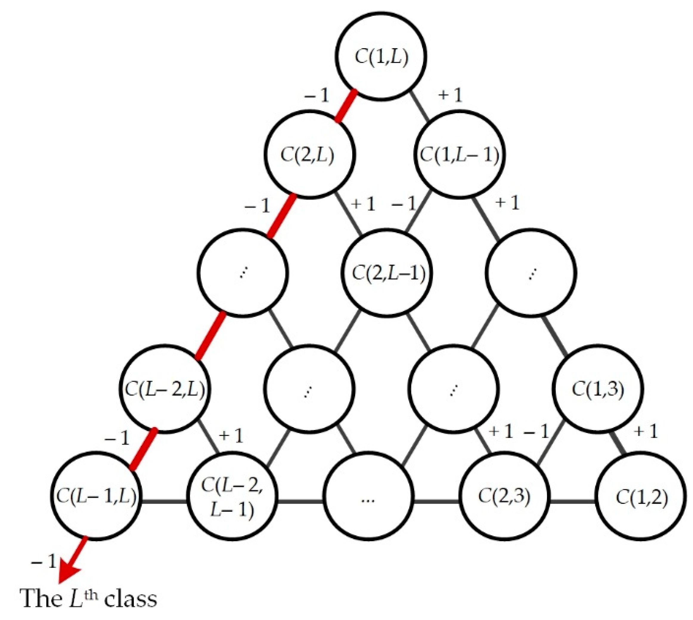
To solve multi-class classification problem with binary classifiers, much research has been conducted, such as winner-takes-all strategy (one-versus-all), max-wins voting strategy (one-versus-one), directed acyclic graph (DAG), and error-correcting output codes (ECOC). Supposing L classes in the classification problem, one-versus-all strategy needs L classifiers, but the computation time of single binary classifier is long because of training the whole samples. The accuracy is also not high because of the biased datasets in two classes. One-versus-one strategy needs L(L–1)/2 classifiers. The number of classifiers increases in quadratic form with the increase in L. For more classifiers, more errors are accumulated. DAG needs (L–1) classifiers, and the upper bound of error accumulation is fixed. No biased datasets exist when training SVM in DAG and the computation time is shorter than one-versus-all or one-versus-one. Although ECOC has developed in recent years, the settings of encoding and decoding need to keep pace with the times, where the numbers of classes in categorical variables of FR is different and the number of classes is also time-varying. Thus, we adopt DAG for the multi-class classification in this study.

DAG for classifying L classes is shown in Figure 4 [37], where C(m,n) represents the binary classifier classifies the mth and nth classes. C(m,n) equaling +1 or −1 represent this sample belongs to nth or mth class. For example, if the outputs of all (L−1) classifiers are −1, this sample is predicted as the Lth class.

4.2.2. SVM for Binary Classification

Supposing a training set Z = {(x_i, y_i), x_i ∊ ℝ^N×p , y_i ∊ {‒1, +1}, i = 1, 2, …, m}, an optimal hyperplane separates the space formed by ${\left\{x_i\right\}}_{i=1}^m$ into two subspaces, where x_i can be divided into two classes in the space. SVM is the method to seek the separating hyperplane ${\omega }^{T}x+b=0$ with the largest margin, which can be expressed as an optimization problem:

$$\begin{array}{l}\min \frac{1}{2}{\Vert \mathit{\omega }\Vert }^2+\xi {\displaystyle \sum _{i=1}^m{\epsilon }_i}\\ s.t. y_i({\mathit{\omega }}^T{\mathit{x}}_i+b)\ge 1-{\epsilon }_i,\\ {\epsilon }_i\ge 0,\\ i=1,2,\dots ,m,\end{array}$$

(11)

where $\xi$ is the penalty factor to balance the minimization of error cost and maximization of margin, and ε_i is the distance from x_i to ${\mathit{\omega }}^T\mathit{x}+b=y_i$.

Problem (11) can be rewritten as Equation (12) using Lagrange multipliers α_i and β_i

$$L(\mathit{\omega },\epsilon ,b,{\alpha }_i,{\beta }_i)=\frac{1}{2}{\Vert \mathit{\omega }\Vert }^2\xi {\displaystyle \sum _{i=1}^m{\epsilon }_i}-{\displaystyle \sum _{i=1}^m{\alpha }_i}\left[y_i\left({\mathit{\omega }}^T\varphi (x_i)+b\right)-1+{\epsilon }_i\right]+{\displaystyle \sum _{i=1}^m{\beta }_i{\epsilon }_i},$$

(12)

where ϕ(x_i) is a mapping function that maps x_i into a high dimensional space. SVM can efficiently perform a non-linear classification using ϕ(x_i).

After partial derivative of Equation (12), problem (11) can be transformed into the dual optimization problem:

$$\begin{array}{l}\min -{\displaystyle \sum _{i=1}^m{\alpha }_i}+\frac{1}{2}{\displaystyle \sum _{i,j=1}^m{\alpha }_i}{\alpha }_j{y}_i{y}_j\kappa (x_i,x_j)\\ s.t. 0\le {\alpha }_i\le C,\\ {\displaystyle \sum _{i=1}^m{\alpha }_i}{y}_j=0,\\ i=1,2,\dots ,m,\end{array}$$

(13)

where $\kappa (x_i,x_j)$ is the kernel function, $\kappa (x_i,x_j)=\varphi {({\mathit{x}}_i)}^{\mathrm{T}}\varphi ({\mathit{x}}_j)$. Radial basis function is the popular kernel function used in SVM,

$$\kappa (x_i,x_j)=\exp \left[-{\Vert x_i-x_j\Vert }^2/(2{\sigma }^2)\right].$$

(14)

Problem (13) is efficiently solvable by quadratic programming algorithms. Then, ω can be solved by

$$\mathit{\omega }={\displaystyle \sum _{i=1}^m{\alpha }_i}{y}_i\varphi ({\mathit{x}}_i).$$

(15)

The SVM classifier function can be written as:

$$C({\mathit{x}}^{\prime })=\mathrm{sgn}\left({\displaystyle \sum _{i=1}^m{y}_i{\alpha }_i\kappa ({\mathit{x}}_i,{\mathit{x}}^{\prime })}+b\right)$$

(16)

The calculation results of $C(\mathit{x}\prime )$ is ±1, where ${\mathit{x}}^{\prime }$ can be classified into one of two classes. Then (L−1) SVM classifiers with DAG can be used in Figure 3 for categorical variable prediction in FR.

5. Case Study

In this section, predicting missing values of FR in KLK2 elevator product (Figure 2), which is a star product in Canny Elevator, Co., Ltd. (Suzhou, China), is taken as a case study to verify the application of the proposed approach in the real world. We explain in this section that:

• The benefit of the proposed framework for predicting the missing values of FR.
• Why we integrate KNN and SVM for continuous and categorical variables prediction, respectively?
• The adaption of proposed approach in the cold- and warm-start scenarios.

5.1. Experimental Setup

5.1.1. Dataset and Compared Methods

To test the performance of the proposed approach, we collected the 91 effective cases of KLK2 elevator as the experimental dataset, in which the design, manufacturing, and install of the elevators have been finished. FRs elicited from these cases are expressed as X, X ∊ ℝ^91×26, p₀ = 10, and p₁ = 16. We randomly sample the values in X to be missing at different missing rates, assuming that each entry is equally likely to be chosen.

We run some of the most commonly used and state-of-the-art methods described in Table 1 to compare against KNN-SVM. The individual methods in this comparison are single methods, including KNN [24,25], BPCA [27], BBPCA [28], GRNN [26], and SVD [30], and composite methods, including KNN-SVD, KNN-GRNN, KNN-BBPCA, KNN with naive Bayes classifier (KNN-Bay) [38], KNN with decision trees model (KNN-Tree) [32], and KNN-SVM. The composite methods are all strengthened by the proposed framework. k = 10 is adopted in KNN in this case study.

5.1.2. Evaluation Metrics

The evaluation metrics used in this study are divided into three patterns, accuracy (RMSE), similarity (Ang, Len, and FSN), and computation time. The known values $\{x_{ij}:(i,j)\in M_0\cup M_1\}$ in X are the ground truth in evaluation. In particular, RMSE between predicted and true values is calculated by

$$\{\begin{array}{c}{\mathrm{RMSE}}_0=\sqrt{\frac{1}{\left|M_0\right|}{\displaystyle \sum _{(i,j)\in M_0}{1}_{\{{\widehat{x}}_{ij}\ne x_{ij}\}}}}\\ {\mathrm{RMSE}}_1=\sqrt{\frac{1}{\left|M_1\right|}{\displaystyle \sum _{(i,j)\in M_1}{({\widehat{x}}_{ij}-x_{ij})}^2}}\end{array}\Rightarrow \mathrm{RMSE}=\sqrt{{\mathrm{RMSE}}_0{}^2+{\mathrm{RMSE}}_1{}^2}$$

(17)

where RMSE₀ and RMSE₁ are RMSEs of categorical and continuous variables, respectively.

Evaluation metrics of similarity include: (1) Ang, sum of angles of the first three principal components calculated for true ($\mathit{\theta }$) and predicted ($\widehat{\mathit{\theta }}$) FRs (ideal value is 0); (2) Len, sum of length of projections of $\mathit{\theta }$ to $\widehat{\mathit{\theta }}$ (ideal value is 3); (3) FSN: mean fraction of the same neighbors from the k nearest neighbors between true and predicted FRs (ideal value is 1).

$$\mathrm{Ang}={\displaystyle \sum _{i=1}^3\arccos \langle {\mathit{\theta }}_i^{},{\widehat{\mathit{\theta }}}_i^{}\rangle },$$

(18)

$$\mathrm{Len}={\displaystyle \sum _{i=1}^3\sqrt{{\displaystyle \sum _{j=1}^3\Vert \upsilon \left({\mathit{\theta }}_i,{\widehat{\mathit{\theta }}}_j\right)\Vert }}},$$

(19)

$$\mathrm{FSN}=\frac{1}{N}{\displaystyle \sum _{i=1}^N\frac{\left|M_i\cap {\widehat{M}}_i\right|}{\left|M_i\cup {\widehat{M}}_i\right|}},$$

(20)

where $\Vert \upsilon \left({\mathit{\theta }}_i,{\widehat{\mathit{\theta }}}_j\right)\Vert$ represents the length of projections of ${\mathit{\theta }}_i$ to ${\widehat{\mathit{\theta }}}_j$; $M_i$ and ${\widehat{M}}_i$ are the k nearest neighbors’ coordinates of ${\mathit{x}}_i$ and ${\widehat{\mathit{x}}}_i$, respectively.

5.2. Experimental Results and Comparison

We run all the methods by missing rate ranging from 10% to 50%. In the following section, we first demonstrate that the methods using the proposed framework are better than single methods. Then, the performance of KNN-SVM is significantly better than the reference methods. Finally, we discuss the influences of cold- and warm-start scenarios in prediction.

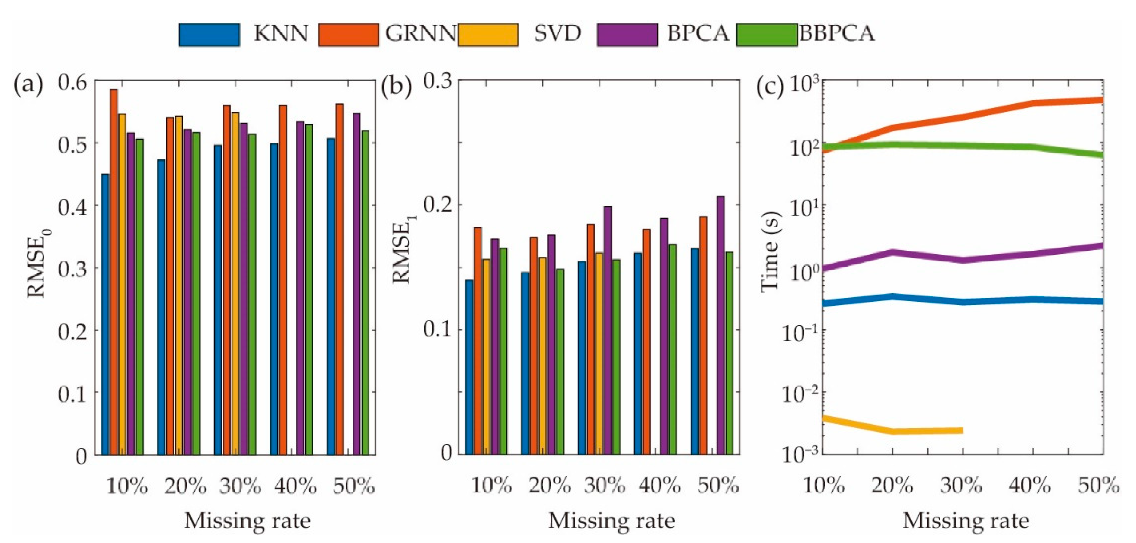
The single methods, KNN, GRNN, SVD, BPCA, BBPCA, are commonly used for continuous variables. For the mixed data type, they put the categories as the continuous numbers instead of labels. The predict values tend to be wildly inaccurate due to rounding errors. As shown in Figure 5a, the performance of all single methods predicting with categorical variables is negative. Compared with continuous variables, RMSE of categorical variables triples.

By comparing the performance of different single methods, KNN outperforms other methods in terms of RMSE₁ (Figure 5b) and has reasonable computation time in real-world applications (Figure 5c). GRNN has poor performance in not only the accuracy but also the computation time. For the shortest computation time of SVD (<0.01 s), there is a fatal flaw that when the missing rate is large, SVD is trapped into a loop without solution. For BPCA, the predicted values of the same requirement are identical, which cannot be applied to predict missing values of FR in product customization. Although BBPCA repairs the gap in BPCA, the performance is still unsatisfactory.

KNN seems to be the best method for regression in the first layer of the proposed framework. Then, we compare the composite methods strengthened by the proposed framework. As shown in

Table 2. Comparison of single and composite methods.

Method	RMSE0			RMSE			Time (s)			Ang
	10%	30%	50%	10%	30%	50%	10%	30%	50%	10%	30%	50%
KNN-GRNN	0.53	0.52	0.56	0.58	0.57	0.59	33	111	222	0.01	0.02	0.05
GRNN	0.59	0.56	0.56	0.61	0.59	0.59	73	254	479	0.03	0.10	0.13
KNN-SVD	0.48	0.51	0.52	0.57	0.57	0.57	0.27	0.29	0.30	0.01	0.03	0.04
SVD	0.55	0.55	_	0.64	0.60	_	<0.01	<0.01	_	0.02	0.04	_
KNN-BBPCA	0.49	0.49	0.49	0.53	0.52	0.54	74	91	88	0.01	0.03	0.04
BBPCA	0.51	0.51	0.52	0.52	0.53	0.54	85	89	62	0.01	0.03	0.05

, handling the continuous and categorical variables of FR separately (in the proposed framework) is beneficial.

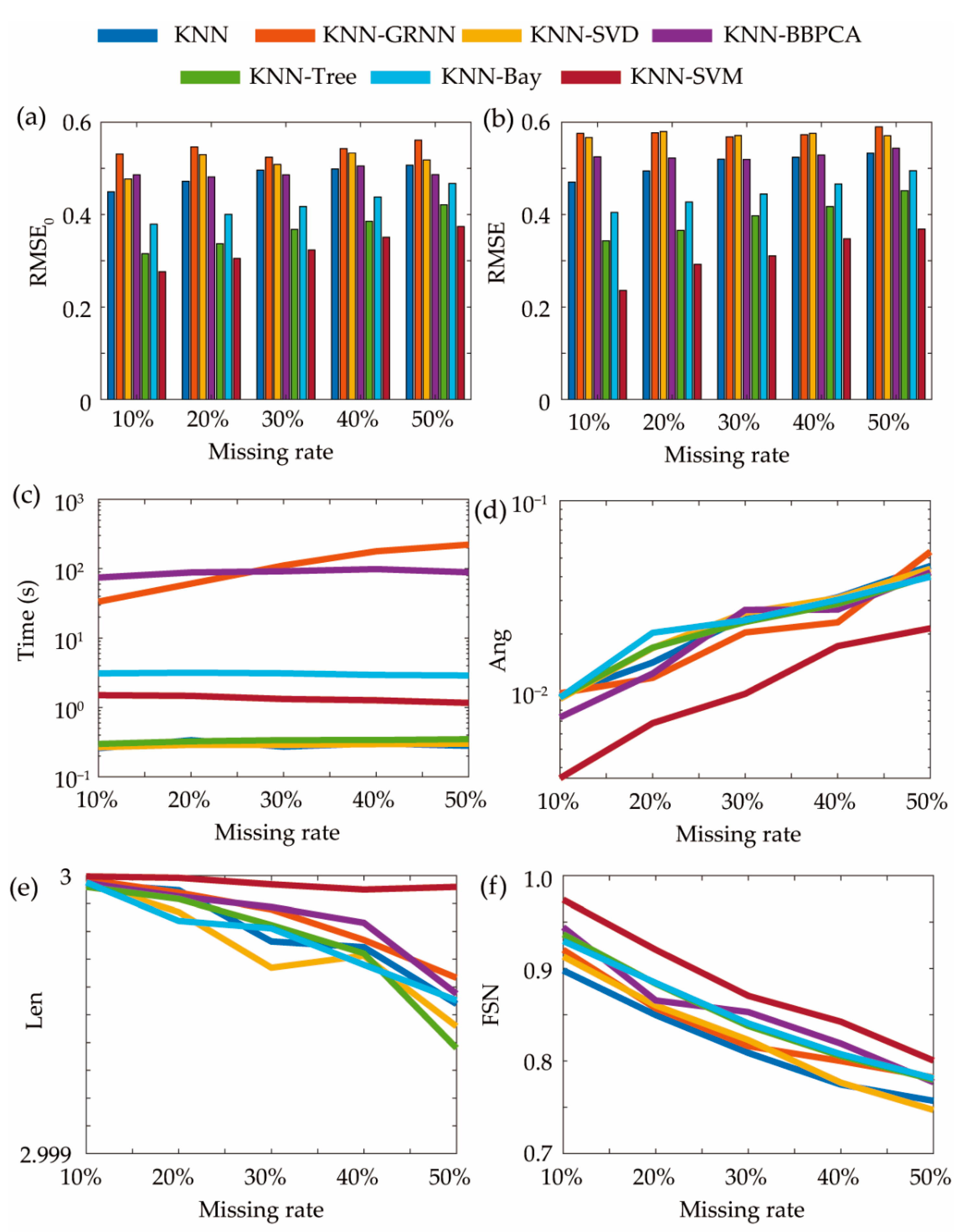
The significant benefit of KNN-GRNN is the shorter computation time than GRNN. After KNN finishes the continuous variable prediction, there are fewer missing values for GRNN to classify; thus, the training time of GRNN is shortened and the total computation time is also shortened. For KNN-SVD, the problem of no solution in high missing rate is solved. As parts of missing values have been predicted, SVD can be operated even with high missing rate. The performance of KNN-BBPCA is a bit better than BBPCA. However, the improvement is not significant for these methods, with average reduction in RMSE of only 3.7% against single methods. It is found that SVD and BBPCA are not feasible for categorical variable prediction. Meanwhile, GRNN costs too long computation time. Thus, we search for other classification methods for predicting the missing categorical variables in the proposed framework. The selected methods include the naive Bayes classifier, decision trees model, and SVM, which are all classic and popular methods in data classification. Some classic binary classifiers are advanced with DAG for multi-class classification (Section 4.2.1).

As shown in Figure 6, all three new classifiers are better than the original three composite methods. In detail, with the same method (KNN) predicting the continuous variables, KNN-SVM outperforms other methods in terms of RMSE as well as Ang, Len, and FSN. KNN-SVD and KNN-Tree are better than KNN-SVM in terms of computation time (Figure 6c), but KNN-SVM results in average reduction in RMSE of 46%, 39%, 30%, and 21% against KNN-SVD, KNN, KNN-Bay, and KNN-Tree, respectively (Figure 6b). SVM usually needs longer computation time for classification, which is its own short slab. Although the computation time is not the shortest, SVM is feasible in the real-world application with around 1.5 s for computation. With the missing rate increasing, the accuracy of prediction decreases, but the performance of similarity in KNN-SVM outperforms the others even in high missing rate. In the proposed framework, KNN-SVM is the most feasible method for practical application.

In addition, we randomly choose 10 and 50 FRs in X for test in cold- and warm-start scenarios. Cold-start scenario refers to the initial scenario for FR prediction, where there are no complete FRs for reference. Usually, experts are required to predict the missing values of FR through their own experience, which is often in the early stage of the new customized product development. Warm-start scenario means there is a number of completed FRs in the resource library. It is the common scenario in product customization.

As shown in

Table 3. Performance of different methods in cold- and warm-start scenarios.

Method	RMSE			Ang			FSN			Time (s)
	10%	30%	50%	10%	30%	50%	10%	30%	50%	10%	30%	50%
Cold-start scenario 1: 10 incomplete FRs without reference
KNN-SVM	0.44	0.52	0.63	0.04	0.09	0.17	_	_	_	1.13	0.51	1.56
KNN-Bay	0.58	0.56	0.78	0.06	0.14	0.26	_	_	_	2.19	1.92	3.19
KNN-Tree	0.56	0.53	0.76	0.11	0.14	0.30	_	_	_	0.19	0.11	0.18
KNN	_	_	_	_	_	_	_	_	_	_	_	_
GRNN	0.59	0.71	0.66	0.04	0.22	0.26	_	_	_	9	11	18
Warm-start scenario 1: 10 incomplete FRs with rest 81 complete FRs for reference
KNN-SVM	0.09	0.18	0.23	4 × 10‒5	1 × 10‒3	1 × 10‒3	1.00	1.00	1.00	0.33	0.69	0.60
KNN-Bay	0.28	0.37	0.38	1 × 10‒3	2 × 10‒3	4 × 10‒3	0.99	0.97	0.96	1.36	1.68	1.81
KNN-Tree	0.32	0.33	0.29	1 × 10‒3	3 × 10‒3	5 × 10‒3	0.99	0.97	0.96	0.24	0.27	0.28
KNN	0.49	0.53	0.50	1 × 10‒3	2 × 10‒3	4 × 10‒3	0.98	0.96	0.96	0.19	0.21	0.20
GRNN	0.63	0.56	0.60	3 × 10‒3	6 × 10‒3	1 × 10‒2	0.98	0.97	0.96	5	15	24
Cold-start scenario 2: 50 incomplete FRs without reference
KNN-SVM	0.31	0.39	0.42	0.01	0.02	0.04	1.00	0.99	0.99	0.50	0.49	0.42
KNN-Bay	0.56	0.59	0.59	0.06	0.10	0.17	0.95	0.86	0.92	3.54	2.77	2.18
KNN-Tree	0.51	0.59	0.55	0.04	0.08	0.14	0.96	0.90	0.90	0.63	0.21	0.16
KNN	0.68	0.62	0.61	0.07	0.15	0.17	0.95	0.92	0.93	0.08	0.07	0.05
GRNN	0.66	0.66	0.67	0.09	0.16	0.21	0.94	0.91	0.91	29	95	127
Warm-start scenario 2: 50 incomplete FRs with rest 41 complete FRs for reference
KNN-SVM	0.14	0.30	0.30	3 × 10‒3	6 × 10‒3	1.2 × 10‒2	1.00	0.95	0.92	0.76	0.78	0.80
KNN-Bay	0.26	0.31	0.36	5 × 10‒3	9 × 10‒3	1.0 × 10‒2	0.98	0.94	0.91	1.87	1.85	1.86
KNN-Tree	0.18	0.33	0.33	6 × 10‒3	9 × 10‒3	1.5 × 10‒2	0.97	0.94	0.91	0.29	0.30	0.30
KNN	0.29	0.53	0.49	5 × 10‒3	9 × 10‒3	1.5 × 10‒2	0.98	0.94	0.90	0.22	0.27	0.23
GRNN	0.46	0.53	0.55	1 × 10‒2	2 × 10‒2	41 × 10‒3	0.97	0.94	0.89	26	73	119

, all methods can only provide the predicted suggestions to managers with low accuracy in the cold-start scenario, especially with few incomplete FRs. For only 10 FRs in the cold-start scenario, the KNN method cannot find the accurate nearest neighbors for prediction, and the metric FSN is not applicable for all methods. Comparing cold-start scenarios 1 and 2, although all FRs are incomplete, more FRs can improve the performance. When the number of incomplete FRs increases, the proposed approach is useful and beneficial, and the predicted results are valuable to managers. Comparing the different start scenarios, KNN-SVM shows better performance in the warm-start scenario. The values of Ang are minimum, which means the predicted values are very similar to the ground truth. If there is a small quantity of incomplete FRs and a mass of complete FRs for reference, the predicted results will be more accurate. It is obvious that KNN-SVM always outperforms other methods and the computation time is acceptable in Table 3. We then make a concrete analysis of the predicted values of a new FR in Section 5.3.

5.3. Case Analysis

A new FR is used to analyze the predicted results using KNN-SVM. We randomly sample the values of this FR to be missing in four cases, where cases 1, 2, 3, 4 contain 2, 5, 7, and 13 missing values, respectively. As shown in

Table 4. Predicted values of a new FR in elevator.

Index	FR	Ground Truth	Predicted Values in Different Cases
			Case 1	Case 2	Case 3	Case 4
r1	Hoisting motor power	10 kW				11 kW
r2	Hoisting rope size	ϕ 10		ϕ 10		ϕ 10
r3	Gear of hoisting machine	Gearless				Gearless
r4	Number of hoisting ropes	2			4
r5	Number of passengers	9			8
r6	Door opening	Front and rear opening				Front and rear opening
r7	Number of stops	15
r8	Counterweight position	Side		Side		Side
r9	Compensating device	Rope				Rope
r10	Number of guides	2			2
r11	Length of hoisting rope	1219		1188.4
r12	Rated capacity	900 kg			840 kg
r13	Speed	4.1 m/s	3.64 m/s		3.64 m/s
r14	Car weight	1053				972.4
r15	Car depth	1328				1328
r16	Car width	1534		1570.6
r17	Car height	2729				2795.8
r18	Shaft depth	2076		2130.3		2119.3
r19	Shaft height	43,086
r20	Shaft width	1997
r21	Door width	939			1043.2	1024.9
r22	Door height	2232	2070.4		2057.2
r23	Door offset distance	0
r24	Machine room height	1638
r25	Headroom height	3386				3974.2
r26	Pit depth	4024				4845.2

, the specific values under four cases are the predicted values using KNN-SVM. Comparing the predicted values with ground truth, we make a concrete analysis to different cases as following.

(1) In cases 1 and 3, where the values of speed (r₁₃) is missing, the predicted value is 3.64 m/s and the difference is acceptable comparing with 4.1 m/s. The shaft height (r₁₉) is 43 m, the time cost is 11.8 vs. 10.5 s, where 1.3 s are negligible for passengers.

(2) The predicted results of categorical variables are accurate against the ground truth. For the binary classification, the predicted values using KNN-SVM are the same as the ground truth in gear of hoisting machine (r₃), door opening (r₆), and counterweight position (r₈). For the multi-class classification, such as hoisting rope size (r₂), number of hoisting roper (r₉), and number of guides (r₁₀), the predicted values are accurate. In addition, the predicted values of hoisting motor power (r₁) are larger than the ground truth. One reason is the missing rate of case 4 is high. From another perspective, the candidate values of r₁ in the product family are {8, 10, 11, 12, 15, 17, 18} kW. Thus, the predicted value of r₁ is acceptable.

(3) Another important requirement is the number of passengers (r₅) with rated capacity (r₁₂). In case 3, r₅ and r₁₂ are missing and the predicted values are 8 and 840 kg, respectively. Although there exist biases, the prediction of the more important requirement r₁₂ is acceptable. These two predicted values are also self-consistent.

(4) The missing continuous variables of FR are predicted using KNN. In the range of the allowable biases, the predicted results (most requirements belong to building information) are valuable and can give suggestions to managers.

(5) The computation time of all cases using KNN-SVM is less than one second, which can provide friendly human–computer interaction in the design activities in product customization.

5.4. Application and Discussion

We have developed a prototype system for elevator customized design based on Java and MySQL, as shown in Figure 7. This design platform has been applied in the elevator customization cooperated with Canny Elevator Co. Ltd. in China. There are four design stages in this design platform, as described in Section 1, and nine design tools in each design stage (Figure 7a). The proposed approach is packaged in the design tool, requirements forecast (Figure 7c), in the requirements modeling stage. In the real-world elevator customized design process, the design tool, requirements elicitation, captures customer requirements and outputs the incomplete CN to the requirements database. FR often has missing values due to incomplete CN, which effects the requirements conversion from FR to design parameters. Traditionally, managers fill in the missing values based on their own knowledge and experience. The imputation results may not fulfil individual customer requirements. After integrating the proposed approach in this design platform, managers can choose the order in the requirements database and view the missing parts in FR, and then automatically obtain the predicted results of the missing values, as shown in Figure 7c.

By performance comparison in Section 5.2 and case analysis in Section 5.3, the predicted results are valuable and effective in the practical design process. The response time of the requirements prediction is less than two seconds, which is also acceptable to managers. The proposed approach is feasible in product customized design, with the following advantages: (1) avoiding managers manually filling in missing values of FR in the design process; (2) the predicted results are similar to the real personalized requirements; (3) this approach solves a potential problem in requirements modeling and can aid product design with rapid response ability.

6. Conclusions

Predicting the missing values of FR is necessary in requirements modeling of product customized design. In this study, a multi-layer framework for prediction is introduced with the KNN’s strengths in continuous variable prediction and SVM’s advantages in categorical variables prediction. A case study on elevator customized design validates the effectiveness and feasibility of the proposed approach. To conclude, the proposed approach reveals the following advantages:

(1) A layered KNN-SVM approach is proposed to predict the missing values of FR efficiently. It focuses on a potential problem arising in requirements modeling, therefore, helps provide the complete function requirements to managers to design products that fulfill individual customer requirements.

(2) The proposed layered KNN-SVM approach, considering continuous and categorical variables synchronously, outperforms other five single and five composite methods in terms of RMSE, Ang, Len, and FSN. Specifically, KNN-SVM results in average reduction in RMSE of 46%, 39%, 30%, and 21% against KNN-SVD, KNN, KNN-Bay, and KNN-Tree, respectively. The computation time of KNN-SVM is always less than two seconds, which is acceptable in practical applications.

(3) The proposed layered KNN-SVM approach also performs better in cold- and warm-start scenarios than other methods. With the number of FRs increasing in the cold-start scenario, KNN-SVM can provide valuable and effective predicted results to managers. In the warm-start scenario, which is the common scenario in practical application, managers can obtain the accurate predicted results using KNN-SVM even in the high missing rate cases.

(4) The case analysis and practical application on real-world customized elevator validate the reasonability and reliability of the proposed layered KNN-SVM approach. The predicted results of categorical variables in FR (such as requirements of hoisting system and cab) are almost the same as the ground truth. The predicted results of continuous variables in FR (such as speed and requirements of building information) can provide valuable results to managers. With the help of the proposed approach, managers can obtain complete and correct requirements and improve the design efficiency in design process.

In the future work, the proposed approach can be improved. For example, the predicted results of continuous variables in FR could be the numerical range, where the single value is less helpful to managers. KNN can be improved or integrated with other state-of-the-art algorithms to improve the performance in the missing continuous variables prediction. Furthermore, more validation is necessitated in other real-world customized products. The developed design tool for manufacturers can be improved for better human–computer interaction. Although this approach is applied in the domain of manufacturing, exploring and researching whether the proposed approach might be useful in filling in missing data in other domains are worthy and meaningful.

References

- Chinese Mechanical Engineering Society. Technology Roadmaps of Chinese Mechanical Engineeringe, 2nd ed.; Science and Technology of China Press: Beijing, China, 2016. [Google Scholar]
- Zhang, S.Y.; Xu, J.H.; Gou, H.W.; Tan, J.R. A research review on the key technologies of intelligent design for customized products. Engineering 2017, 3, 631–640. [Google Scholar] [CrossRef]
- Neira-Rodado, D.; Ortíz-Barrios, M.; De la Hoz-Escorcia, S.; Paggetti, C.; Noffrini, L.; Fratea, N. Smart product design process through the implementation of a fuzzy Kano-AHP-DEMATEL-QFD approach. Appl. Sci. 2020, 10, 1792. [Google Scholar] [CrossRef] [Green Version]
- Rodríguez-Parada, L.; Mayuet, P.F.; Gámez, A.J. Custom design of packaging through advanced technologies: A case study applied to apples. Materials 2019, 12, 467. [Google Scholar] [CrossRef] [PubMed] [Green Version]
- Lee, C.-H.; Chen, C.-H.; Lin, C.; Li, F.; Zhao, X. Developing a quick response product configuration system under Industry 4.0 based on customer requirement modelling and optimization method. Appl. Sci. 2019, 9, 5004. [Google Scholar] [CrossRef] [Green Version]
- Jimeno-Morenilla, A.; Sánchez-Romero, J.S.; Salas-Pérez, F. Augmented and virtual reality techniques for footwear. Comput. Ind. 2013, 64, 1371–1382. [Google Scholar] [CrossRef] [Green Version]
- Gao, X.J.; Shi, M.L.; Song, X.G.; Zhang, C. Recurrent neural networks for real-time prediction of TBM operating parameters. Automat. Constr. 2018, 98, 225–235. [Google Scholar] [CrossRef]
- Suh, N.P. The Principle of Design; Oxford University Press: Oxford, UK, 1990. [Google Scholar]
- Yan, W.-J.; Chiou, S.-C. Dimensions of customer value for the development of digital customization in the clothing industry. Sustainability 2020, 12, 4639. [Google Scholar] [CrossRef]
- Clarkson, J.; Eckert, C. Design Process Improvement; Springer: London, UK, 2005. [Google Scholar]
- Adams, K.M. Nonfunctional Requirements in Systems Analysis and Design; Springer: Cham, Switzerland, 2015. [Google Scholar]
- Guo, Q.; Xue, C.Q.; Yu, M.J. A new user implicit requirements process method oriented to product design. J. Comput. Inform. Sci. Eng. 2019, 19, 011010. [Google Scholar] [CrossRef]
- Qi, J.Y.; Zhang, Z.P.; Jeon, S.M.; Zhou, Y.Q. Mining customer requirements from online reviews: A product improvement perspective. Inform. Manag. 2016, 53, 951–963. [Google Scholar] [CrossRef]
- Yan, Y.W.; Huang, C.C.; Wang, Q.; Hu, B. Data mining of customer choice behavior in internet of things within relationship network. Int. J. Inform. Manag. 2018, 50, 566–574. [Google Scholar] [CrossRef]
- Jiang, H.M.; Kwong, C.K.; Park, W.Y.; Yu, K.M. A multi-objective PSO approach of mining association rules for affective design based on online customer reviews. J. Eng. Des. 2018, 29, 381–403. [Google Scholar] [CrossRef]
- Zhou, F.; Jiao, J.R.; Linsey, J.S. Latent customer needs elicitation by use case analogical reasoning from sentiment analysis of online product reviews. J. Mech. Des. 2015, 137, 071401. [Google Scholar] [CrossRef]
- Song, W.Y.; Ming, X.G.; Xu, Z.T. Integrating Kano model and grey–Markov chain to predict customer requirement states. Proc. Inst. Mech. Eng. B 2013, 227, 1232–1244. [Google Scholar] [CrossRef]
- Raharjo, H.; Xie, M.; Brombacher, A.C. A systematic methodology to deal with the dynamics of customer needs in quality function deployment. Expert. Syst. Appl. 2011, 38, 653–3662. [Google Scholar] [CrossRef]
- Min, H.; Yun, J.; Geum, Y. Analyzing dynamic change in customer requirements: An approach using review-based Kano analysis. Sustainability 2018, 10, 746. [Google Scholar] [CrossRef] [Green Version]
- Fan, W.; Li, J.; Ma, S.; Tang, N.; Yu, W. Towards certain fixes with editing rules and master data. VLDB J. 2012, 21, 213–238. [Google Scholar] [CrossRef] [Green Version]
- Grzymala-Busse, J.Z.; Goodwin, L.K.; Grzymala-Busse, W.J.; Zheng, X. Handling missing attribute values in preterm birth data sets. In Rough Sets, Fuzzy Sets, Data Mining, and Granular Computing, Proceedings of the International Workshop on Rough Sets, Fuzzy Sets, Data Mining, and Granular-Soft Computing, Regina, SK, Canada, 31 August–3 September 2005; Springer: Berlin, Germany, 2005; pp. 342–351. [Google Scholar] [CrossRef] [Green Version]
- Schneider, T. Analysis of incomplete climate data: Estimation of mean values and covariance matrices and imputation of missing values. J. Clim. 2001, 14, 853–871. [Google Scholar] [CrossRef]
- Honaker, J.; Gary King, G.; Blackwell, M. Amelia II: A program for missing data. J. Stat. Softw. 2011, 45, 1–47. [Google Scholar] [CrossRef]
- Zhang, S. Nearest neighbor selection for iteratively kNN imputation. J. Syst. Softw. 2012, 85, 2541–2552. [Google Scholar] [CrossRef]
- Kim, K.; Kim, B.; Yi, G. Reuse of imputed data in microarray analysis increases imputation efficiency. BMC Bioinform. 2004, 5, 160. [Google Scholar] [CrossRef] [Green Version]
- Gheyas, I.A.; Smith, L.S. A neural network-based framework for the reconstruction of incomplete data sets. Neurocomputing 2010, 73, 16–18. [Google Scholar] [CrossRef]
- Shigeyuki, O.; Sato, M.A.; Takemasa, I.; Monden, M.; Matsubara, K.; Ishii, S. A Bayesian missing value estimation method for gene expression profile data. Bioinformatics 2003, 19, 2088–2096. [Google Scholar] [CrossRef]
- Meng, F.; Cai, C.; Yan, H. A bicluster-based Bayesian principal component analysis method for microarray missing value estimation. IEEE J. Biomed. Health Inform. 2014, 18, 863–871. [Google Scholar] [CrossRef]
- Stekhoven, D.J.; Bühlmann, P. MissForest—Non-parametric missing value imputation for mixed-type dat. Bioinformatics 2012, 28, 112–118. [Google Scholar] [CrossRef] [PubMed] [Green Version]
- Troyanskaya, O.; Cantor, M.; Sherlock, G. Missing value estimation methods for DNA microarrays. Bioinformatics 2001, 17, 520–525. [Google Scholar] [CrossRef] [Green Version]
- Dinh, T.; Huynh, V.N. k-CCM: A center-based algorithm for clustering categorical data with missing values. In Modeling Decisions for Artificial Intelligence, Proceedings of the International Conference on Modeling Decisions for Artificial Intelligence, Palma de Mallorce, Spain, 15–18 October 2018; Springer: Cham, Switzerland, 2018; pp. 267–270. [Google Scholar] [CrossRef]
- Bertsimas, D.; Pawlowski, C.; Zhuo, Y.D. From predictive methods to missing data imputation: An optimization approach. J. Mach. Learn. Res. 2017, 18, 7133–7171. [Google Scholar]
- Ye, C.; Wang, H.Z.; Li, J.Z.; Gao, H.; Cheng, S.Y. Crowdsourcing-enhanced missing values imputation based on Bayesian network. In Database Systems for Advanced Applications, Proceedings of the International Conference on Database Systems for Advanced Applications, Dallas, TX, USA, 16–19 April 2016; Springer: Cham, Switzerland, 2016; pp. 67–81. [Google Scholar] [CrossRef]
- Wang, H.; Qi, Z.; Shi, R.; Li, J.; Gao, H. COSSET+: Crowdsourced missing value imputation optimized by knowledge base. J. Comput. Sci. Technol. 2017, 32, 845–857. [Google Scholar] [CrossRef]
- Zhang, S.; Li, X.; Zong, M.; Zhu, X.; Cheng, D. Learning k for kNN classification. ACM Trans. Intell. Syst. Technol. 2017, 8, 43. [Google Scholar] [CrossRef] [Green Version]
- Shakhnarovish, G.; Darrell, T.; Indyk, P. Nearest-neighbor Methods in Learning and Vision; MIT Press: Cambridge, MA, USA, 2005. [Google Scholar]
- Chen, P.; Liu, S. An improved DAG-SVM for multi-class classification. In Proceedings of the International Conference on Natural Computation, Tianjin, China, 14–16 August 2009; IEEE: Los Alamitos, CA, USA, 2009; pp. 460–462. [Google Scholar]
- Hruschka, E.R.; Hruschka, E.R.; Ebecken, N.F.F. Bayesian networks for imputation in classification problems. J. Intell. Inf. Syst. 2007, 29, 231–252. [Google Scholar] [CrossRef]
Figure 1.
Design activities in product customization and workflow of requirements modeling.
Figure 2.
Functional requirements of a customized elevator.