
Human Health Impact Analysis of Contaminant in IoT-Enabled Water Distributed Networks


1
Engineering Department, Faculty of Computing, Engineering and Built Environment, Birmingham City University, Birmingham B4 7XG, UK
2
Urban Water Networks Department, TPF Getinsa Eurostudios, 28028 Madrid, Spain
*
Author to whom correspondence should be addressed.
†
These authors contributed equally to this work.
Appl. Sci. 2021, 11(8), 3394; https://0-doi-org.brum.beds.ac.uk/10.3390/app11083394
Submission received: 23 February 2021
/
Revised: 1 April 2021
/
Accepted: 6 April 2021
/
Published: 10 April 2021
(This article belongs to the Special Issue Advancements in Biomonitoring and Remediation Treatments of Pollutants in Aquatic Environments)
Abstract
:This paper aims to assess and analyze the health impact of consuming contaminated drinking water in a water distributed system (WDS). The analysis was based on qualitative simulation performed in two different models named hydraulic and water quality in a WDS. The computation focuses on quantitative analysis for chemically contaminated water impacts by analyzing the dose level in various locations in the water network and the mass of the substance that entered the human body. Several numerical experiments have been applied to evaluate the impact of water pollution on human life. They analyzed the impact on human life according to various factors, including the location of the injected node (pollution occurrence) and the ingested dose level. The results show a significant impact of water contaminant on human life in multiple areas in the water network, and the level of this impact changed from one location to another in WDSs based on several factors such as the location of the pollution occurrence, the contaminant concentration, and the dose level. In order to reduce the impact of this contaminant, water quality sensors have been used and deployed on the water network to help detect this contaminant. The sensors were optimally deployed based on the time-detection of water contamination and the volume of polluted water consumed. Numerical experiments were carried out to compare water pollution’s impact with and without using water quality sensors. The results show that the health impact was reduced by up to 98.37% by using water quality sensors.
1. Introduction
One of the fundamental human rights of all human beings, regardless of their race, nationality, religion, and beliefs, is to have pure and safe drinking water [1]. At a fundamental level, daily consumption requires a minimum amount of water for survival, and thus access to a particular form of water is necessary for life [2]. Water has a much more significant impact on health and well-being. However, concerns in many subjects, such as the quality and quantity of water supplied, are essential in determining the health of individuals and entire communities [3]. Water utilities’ fundamental duties are to provide and distribute water to customers of an acceptable quality, quantity, and pressure through the entire water distributed system (WDS) [4]. The usable water is at first treated to meet the drinking water quality standards before delivery [5]. Because of the spatial scale and the high complexity of water distributed networks, adverse accidental incidents commonly occur. For this unwanted event, the growth of infectious diseases begins with biological and chemical contaminants in drinking water [6]. The use of contaminated drinking water and poor sanitation is directly related to the transmission of diseases and epidemics, for example, diarrhea, polio, dysentery, cholera, hepatitis, gastric ulcers, pneumonia, and pulmonary disease [7]. Water supplies may contain various non-biological contaminants, including silica, sodium, sulfur, ammonia, and chlorine. In addition to these contaminants, microbiological contaminants in drinking water at the stage of consumption represent another problem of water quality. Poor drinking water quality significantly affects consumers’ health [8]. In recent years, many developing countries have set public health goals to reduce waterborne diseases and develop safe water resources, and the situation has improved slightly. This somewhat improved situation can be further exacerbated by increased water demand and lower water availability due to population growth and economic growth. Understanding the factors that influence the quality of drinking water is also a necessary step in making the right decisions about protecting and managing the quality of drinking water [9]. In general, the quality of drinking water is affected by the variety of water sources, the treatment in predistribution water treatment plants, the water distribution system, and the containers or tanks used for water storage and household filters. However, in rural areas and small municipalities, drinking water is generally pumped directly from wells or rivers, lakes, and reservoirs without adequate treatment [10]. Therefore, the quality of water sources plays a fundamental role in determining the quality of drinking water.
Protecting water source quality, which plays a crucial role in providing safe drinking water, usually requires the combined efforts of many partners, such as water managers, industrial plants, water supply, communities, and the public [11]. Evaluation of individual water quality parameters may not give a good understanding of water quality between partners with different scientific backgrounds. On the other hand, the traditional method, even by water quality experts, can also cause subjective judgments and prejudices. To solve the problems associated with characterizing and interpreting the state of water quality, various indicators of water quality have been developed to convert the levels of water quality parameters into a numerical index integrated using mathematical tools [12]. Many factors are taken into account when calculating these water quality indicators, and the two most important factors are the time from the incidence of contamination to the water delivery to the customer and the load and concentration of pollution taken from the tap water by the user.
The main contributions of this paper are as follows: (1) Propose a health impact analysis model based on hydraulic and water quality models. (2) Analyze the impact of water contamination based on its occurrence locations and ingested dose level. (3) Reduce the contamination impact using water quality sensors that were optimally deployed based on the time of detection and volume of contaminated water.
2. Related Work
The use of a feasible and effective method of assessing the quality of drinking water is essential to achieve reliable results and to facilitate informed decision-making. Since the 1960s, when Horton developed the first water quality index (WQI), many methods of assessing water quality have been proposed [13,14,15]. The rapid development of water quality assessment methods improves our understanding of water quality either by a single numeric number or by a more sophisticated interpretation of water quality characteristics [16].
Abtahi et al. [11,17] proposed Drinking Water Quality Indicators (DWQIs) to understand the general status of drinking water quality in water networks. The DWQI method works to classify the variety of drinking water sources based on a comparison of the inputs measured values of the water quality parameters with the standard fundamental values (benchmark). The DWQI scores classify the quality of drinking water into five different categories: excellent, good, fair, marginal, and weak. The results showed that the DWQI is a stable, flexible, simple, and reliable indicator, and it could be used as an essential method for characterizing the quality of the drinking water supply. Likewise, Akter et al. [18] used the weighted arithmetic WQI approach to provide details on water quality in Bangladesh. The WQI method converts massive numbers of water quality variables into digital numbers, and it is useful for understanding the water quality, making it one the most common methods for measuring water quality with some limitations. Furthermore, Ba and McKenna [19] developed a time series monitoring and event detection method for water quality. This method composites an affine projection algorithm and an autoregressive (AR) model to predict the time series of water quality. In order to assess the existence of contamination events or not, they used the online change point detection methods for estimated residuals. Most recently, Braun et al. [20] studied the impact of demand uncertainties on the water age in a network model and applied polynomial chaos expansion (PCE) on two real networks. The results show the PCE performs considerably better for a fixed number of simulations, while perturbation approaches are not appropriate for this task. Moreover, the scale of the network has been shown to have a significant impact on the maximum water age.
Nonetheless, these approaches to evaluating water quality rely on water quality criteria for classifying water quality. Therefore, what matters is establishing water quality standards while taking into account specific regional local water quality conditions, the context of water quality indicators, and the health problem [21]. It would be difficult to fully understand the water quality without incorporating these issues into the water quality standards. In contrast, the rapid growth of methods to evaluate water quality is also very promising [22].
Contrary to the rapid development of water quality assessment strategies, assessing human health risks relies mainly on the model suggested by the United States Environment Protection Agency (USEPA) or updated USEPA models. However, the slow development of the evaluation model does not impede health risk assessment activities. Over the past three decades, increasingly more health risk assessment studies have been performed. Researchers slowly recognized the vital role that public health risk assessment plays in effective water quality control and consumer safety, instead of waterborne diseases. For example, Chen et al. [23] used the triangular Fuzzy Number Approach to consider inconsistencies in the health risk assessments provided by the USEPA. The results showed that the health risk assessment model is successful in quantifying risk uncertainty with lower complexity. Moreover, the findings in this paper help managers mitigate possible safety risks and provide new insight to address water uncertainties. Another study by Zhang et al. [24] where strontium (Sr) is detected in drinking water was studied through a monthly sampling strategy in twelve locations in Xi’an, Northwest China. A Monte Carlo simulation was carried out in a safety risk assessment for various age groups and exposure routes. The results of this study could be useful in developing possible risk control. In the study by Ali et al. [25], organophosphate pesticide concentrations (OPPs) were determined in drinking water samples obtained in the Peshawar Basin, Pakistan. The findings showed the highest contamination for methamidophos was detected among OPPs, while the lowest was found for dichlorvos. This study, therefore, recommends stopping the use of shallow drinking water and using deep groundwater at depths >98 m, which showed relatively less pollution. Joshi et al. [26] assessed the combination of drinking water quality and meteorological factors with the incidence of enteroviral diseases among children in seven Korean metropolitan provinces. They concluded that drinking water quality was one of the main determinants of enteroviral diseases.
Full awareness of the water quality status and the possible impacts on human health is the first step towards sustainable governance of water quality [27]. Adimalla and Li [28] assessed the quality of groundwater for consumption and irrigation and estimated the possible adverse impact on health for consumers in the rapidly urbanizing areas in Telangana State, India. Results showed that, due to the use of highly contaminated drinking water with nitrate and fluoride in the study region, children were more vulnerable to health risk. Kumar et al. [29] proposed a method using sensitivity analysis (SSA) to assess the relative impact of inputs in estimating the dose to safety. This method is useful in evaluating the ambiguity and vulnerability of parameters in the input health hazard framework. Shahra and Wu [30] proposed a sensor placement using an evaluations algorithm (EA). The proposed method uses multiple objectives—the volume of the contaminated water (VCW) and time detection (TD)—to find the optimal sensor placements. Two real case studies of WDNs were used to evaluate the effectiveness of the proposed method. The results showed the ability of the proposed method to maximize the coverage of the deployed sensors and reduce the time detection of the water contaminant. Ung et al. [31] used Monte Carlo and identification methods for sensor placement. It calculates a ranked list of potential contamination location nodes and contamination times using binary responses from sensors. The backtracking algorithm is used to determine the source identification. The locations of sensors that are best suited for allocating the source of contamination are determined using a greedy algorithm and a local search algorithm, all of which are combined with a Monte Carlo approach. The proposed method was tested using a real French water network with 2500 nodes. In another study, Hooshmand et al. [32] proved the quality of the two expectation-based models (IBM and IPM) to identify the appropriate configuration of the sensors. These expectation models are extended to include the value at risk (VaR), worse case, and conditional VaR measures (CVaR). Numerical experiments on a real network of WDNs have shown that the optimal sensor placement of CVaRIBM causes an increase of approximately 18.5% in the expectation values compared with the optimal sensor of WorstIBM. The optimal sensor placement of CVarIBM causes increases of 36% in the value of the worst case compared with the values of IBM and VaRIBM. Santonastaso et al. [33] used three different methods to find the detection quality point in WDS; these three methods are based on topology, optimization, and empiricism. The comparisons showed that the widely used empirical approach of the water utility is unsatisfactory. Although the optimization-based approach performs significantly better, it is difficult to implement because it necessitates a calibrated hydra. Due to its simplicity compared to the optimization-based approach, the topological approach proves to be successful, and it can be easily adopted by water utilities to determine the location for quality detection points. Hu et al. [34] conducted a theoretical analysis of an optimal scheduling problem before demonstrating that the valve and hydrant scheduling are NP-complete. Following that, they propose a multi-objective optimization model to respond to the contaminant. The proposed model focuses on two opposing goals: first, minimizing the volume of contaminated water exposed to the public, and second, minimizing the hydrant and valves’ operational costs. The validity of the proposed model is demonstrated by two different water networks.
3. Materials and Methods
3.1. Materials
3.1.1. Case Study
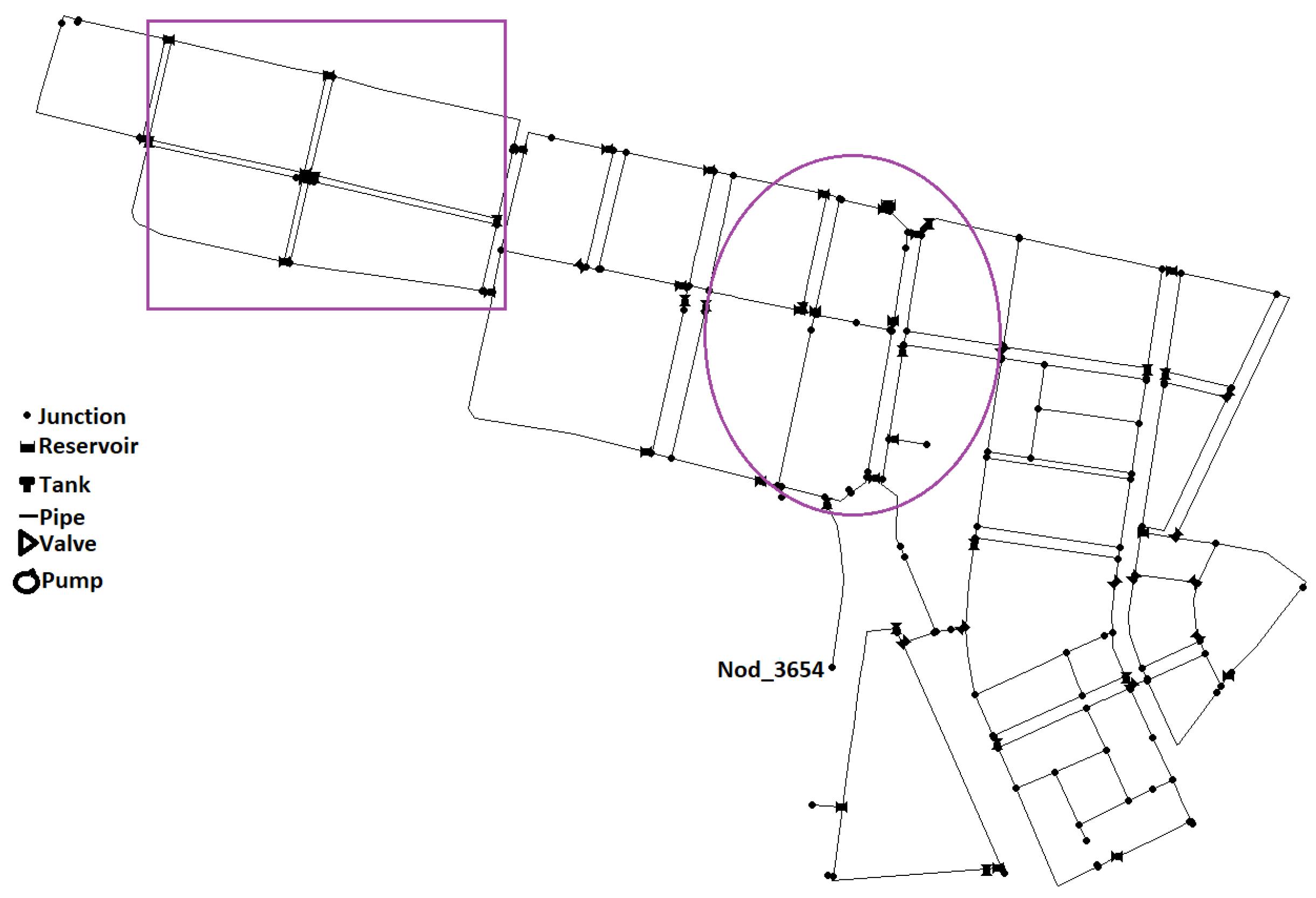
The real case study represents the drinking water network distributed in a district of Madrid City, specifically the city center, Spain. It has dimensions of X = 1.5 Km, Y = 1.03 Km, as shown in Figure 1. It includes one reservoir, two pumps, fifty-five valves, three-hundred-and-ten pipes, and three-hundred-and-twelve junctions. This study was carefully chosen to include different cases in terms of water demand. The three cases were divided based on the water demand, and they are labeled in the case study by a circle, square, and node_3654. Whereas the water demand is considered high in the center and the areas near the source of drinking water (labeled by the circle in Figure 1), in the isolated regions (not connected to the rest of the network) the water demand is minimal, as at Nod_3654 shown in Figure 1. There are also other areas related to the primary system but with a medium need for drinking water, as labeled by a square in the case study presented in Figure 1. Based on these three different cases, in this study only chemical water contaminant is used, so it is generated and spread in this network for 8 h, see Section 3.2.1 for more details. Through this, the impact of water contaminants on human health will be calculated and analyzed in all the previous cases that have been mentioned above.
3.1.2. Tools
The analysis of this paper was performed with TEVA-SPOT [35], which uses the toolkit of an EPANET programmer (2.00.12) for hydraulic and water quality modeling in a WDS. TEVA-SPOT was created by the National Homeland Security Research Center of the USEPA to include the ability to determine the impact of deliberate and accidental releases of a contaminant into a WDS. It is one of the tools that can be conveniently and effectively used in a water network model to determine the impacts of injections at any or all nodes. The TEVA-SPOT included the ability to monitor contaminant mass using the concentration results given by EPANET to allow a better understanding of the distribution of a contaminant in a network after injection and to improve quality control for simulations [36].
EPANET is a software program used to model water delivery networks around the globe. It was developed as a method to understand the movement and fate of components of drinking water within distribution systems. It can be used in distribution system analysis for many different types of applications. It can also be used to model risks of pollution and determine resistance to threats of safety or natural disasters [37].
3.2. Methods
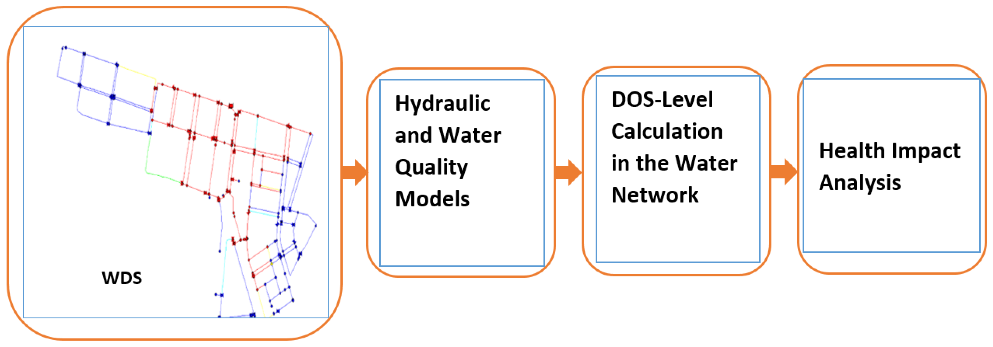
The risk assessment approach relies on the determination of the safety and life-threatening consequences of water supply involving contaminants. The proposed model of health impact analysis encompasses various phases: contaminants generation, dose level calculation, and health impact analysis as shown in Figure 2, more details of these phases are given in the following subsections.
3.2.1. Contaminant Generation
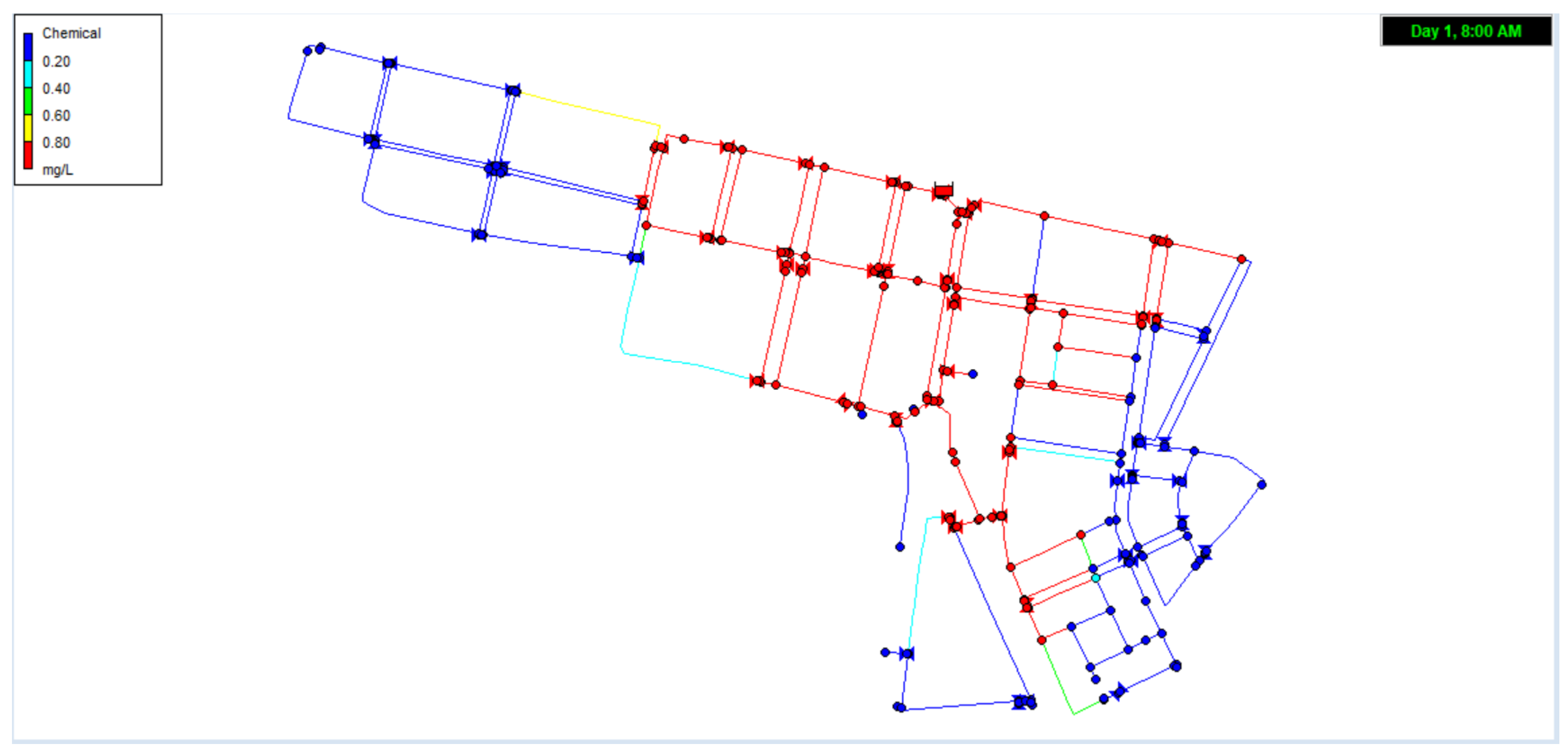
In the first phase, the water contaminants are generated and start to propagate in the system (see Figure 3). Chemical/toxin contaminants are used to represent the events in this study. For these contaminants, the health impacts are based on the lethal dose (LD50). Therefore, some parameters need to be set for this kind of contaminant, such as LD50, resulting in death to 50% of the population; body weight; and others. All parameter values required for the contaminant have been set up based on the EPA’s guidance [35], and they are summarized in Table 1. Another point that needs clarification is how the water contaminant spread in the water network for eight hours. Figure 3 depicts all nodes in the water network model that have been color-coded based on the concentration level of the chemical contaminant that would result across the network given an injection node at the water source (reservoir). The legend on the left hand side of the map provides the scale of the contaminant for both links and nodes, where the red color represents the high level of the contaminant concentration and the blue shows the low level of the same contaminant.
3.2.2. Dose Level Calculation
Hydraulics and water quality models are performed in a water pipeline network for predicting spatial and temporal changes in the concentration of contaminants in the water network. Dose delivered to a subsection of the water network which is supplying N people needs to be calculated, and its level in each branch needs to be determined. For this, Equation (1) was used and applied [38].
where
- = load of substance delivered to people from i sub-network (pipe),
- = concentration of contamination in water at time (t),
- = Water demand in section i at a time (t), and
- t = Exposure time.
Based on Davis et al. [39], a procedure for evaluating a simple contaminant concentration linked to an adverse outcome was illustrated. Equation (2) was used to determine the concentration of the contaminant ingested [36]:
where is the contaminant concentration, q is a constant for the water ingestion rate, M is the mass of the contaminant, and Q is the volume of the water usage rate. The target dose of a person for a specific contaminant can be calculated from the dose–response data available for the contaminant as well as the individual’s body mass. The dose values are typically expressed in units of mg per kg of body mass. The maximum number of people (N) who can receive an ingested dose (d) equals the mass ingested divided by the dose as shown in Equation (3) [36]:
where N represents the population served as represented by the model of the water distribution system, and d is the dose of the target contaminant resulting from the ingestion of tap water. The target dose of a person for a specific contaminant can be calculated from the available dose response data for the contaminant along with the body mass of the individual. The lethal dose (50), for example, is the dose at which 50 percent of the population that receives such a dose dies, this defines the 50 for a contaminant. Using the contaminant-specific 50 information and the mean body mass of the population, a target dose for a contaminant () can be determined as shown in Equation (4):
3.2.3. Health Impact Analysis
Health impacts are measured in terms of the number of people exposed to or affected by the contaminated water. Potential public health impacts on contaminants can differ dramatically across networks. Public health impacts increase with the network population for contaminants with high toxicities, particularly for the scenarios with injection locations that have consequences near the upper end of the distribution. On the other hand, for less toxic contaminants potential public health impacts have not been shown to be sensitive to the network population, even those across the network that differ by more than a factor of population size. This is because contaminants with low toxicity appear to create localized impacts that are constrained by the mass of the available contaminant rather than the contaminants with high toxicity. The public health impact is analyzed and evaluated by calculating the mass of the substance to enter the body using Equation (5):
where q is the volume of consumed water and is the contamination concentration. G is the average weight of the human body during the exposure, and t is the duration of exposure. The risk will be ignored if the value of is too small relative to the tolerable daily intake. The volume of consumed water is represented using Equation (6):
where is the volume of the water at node n for event e, is the threshold hazard concentration, and is the concentration at node n for event e. is the contaminant concentration, (t) denotes the water demand at node i at a time step, and t represents the time step interval. The volume of contaminant water for all event scenarios is calculated based on Algorithm 1.
| Algorithm 1 Calculating the volume of the contaminant water |
| 1: Generate Contamination Scenarios (S). |
| 2: Select one scenario (C) from S. |
| 3: WHILE ( C ≤ S) |
| 4: Simulate Hydraulic and Quality models. |
| 5: If (Contamination Concentration(CC) > > Threshold) |
| 6: Contaminate water volume (q) ← cc × Δt × demand |
The research methodology represented in Figure 2 can be summarized as follows:
- Generate and simulate water contamination propagation on the pipeline networks (WDS).
- Develop the hydraulic and water quality models of the pipeline networks.
- Calculate dose level delivered to one section of the water network, which is supplying N people using Equation (1).
- Evaluate the health impact based on the calculation of the mass of the substance entering the body using Equation (5).
4. Results and Discussion
4.1. Health Analysis Results
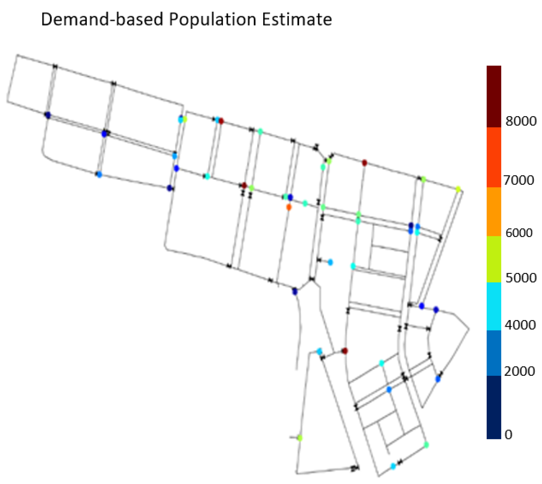
To show the results from the Madrid case study described in the Section 3.1.1, we start explaining the distribution of contaminants based on the water demand of the network. In this work, we used the demand-based method to define the number of water gallons used by each person per day (GPD) to define the distribution of the population. Figure 4 depicts that high demand is focused on the center of the network, while low demand is focused on the top left of the water network. Various demand levels are represented by different colors in the map, where blue represents the deficient water demand and dark red represents the high water demand.
In this study, public health impacts have been described as the size of the population receiving a contaminant intake dose above a certain level. To calculate this, we simulate the impact of water contaminants in different locations in the case study used in this work, as shown in Figure 5, and then investigate the impact of the contaminant for each location. Table 2 presents the impacts of the contaminant based on where the contaminant has occurred (injected node location) in the case study. This table shows the essential properties of the water contaminants, such as the location, max concentration, max individual dose, and the number of estimated infected people. Referring to Table 2, the locations of the contaminant are selected carefully to include all cases, where Loc.6 represents that the contaminants occurs at the source of the water (Reservoir). This kind of contaminant has a high impact on the number of water nodes in WDS, which leads to a high number of people becoming infected from this contaminant. While Loc. 1 means that a contaminant is present in one of the isolated areas in the case study (see Figure 5), these areas labeled by nod_3654; in these areas, the impact of the contaminant on water nodes is small, which leads to a small number of people being affected by this contaminant.
From Table 2, we note that the location of the injected node is the essential property of contamination as it recorded a high number of estimated infected people (146,729) when the contaminant occurred in the water source (Loc. 6), even though the contaminant was carrying a lower concentration. While very few infected people, ranging from zero to 2750 people, were recorded when the contaminant occurred in isolated locations (Loc. 2) that have a low population, the contamination was recorded at a higher concentration. On the other hand, the remaining locations—Loc. 3, Loc. 4, and Loc. 5—recorded a number of different infected people with a variable contaminant concentration as well. To examine and investigate the impact of water contaminant based on its occurrence in more details, two different cases were chosen (Loc. 2 and Loc. 6), and the extent of the impact is explained in detail as follows.
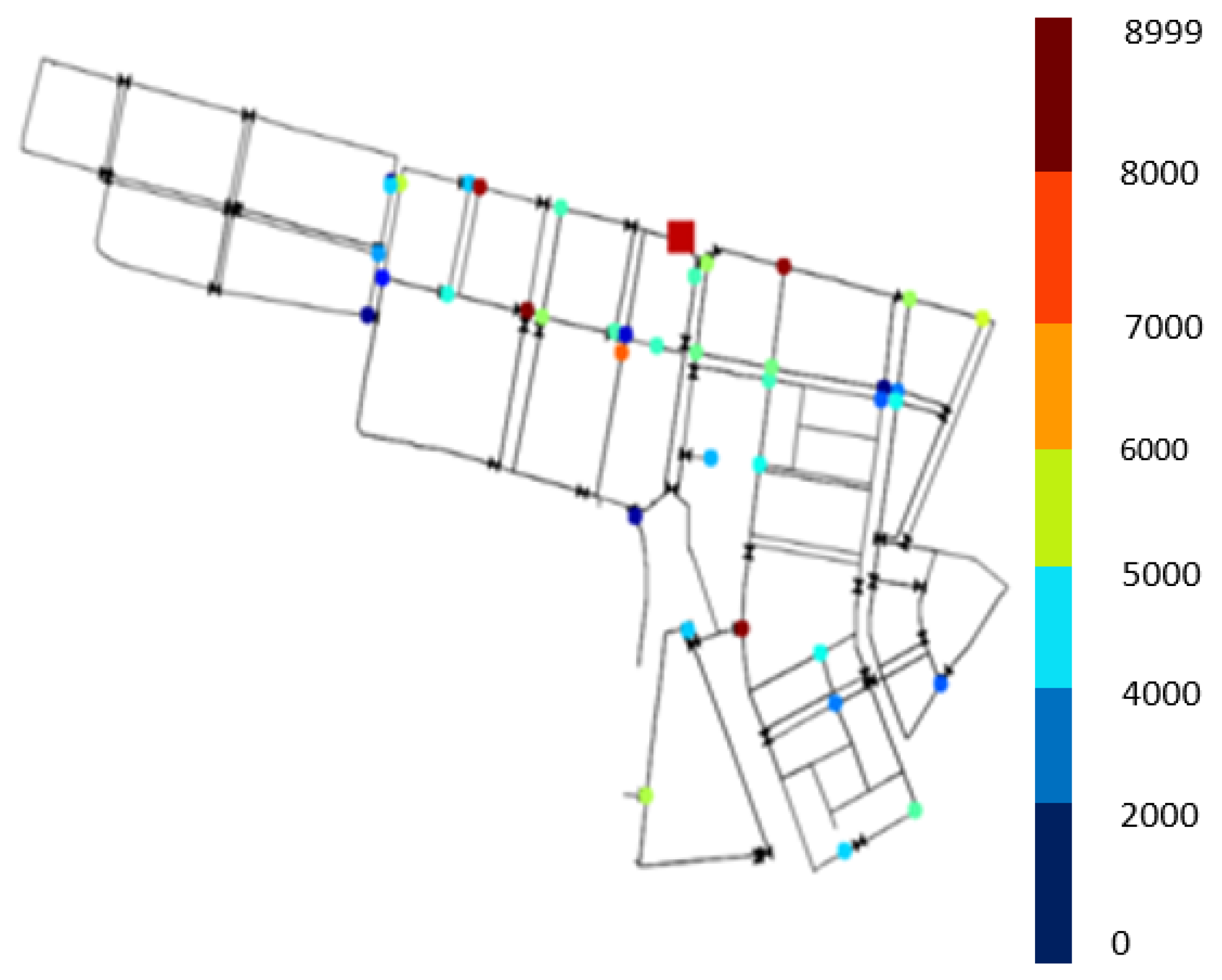
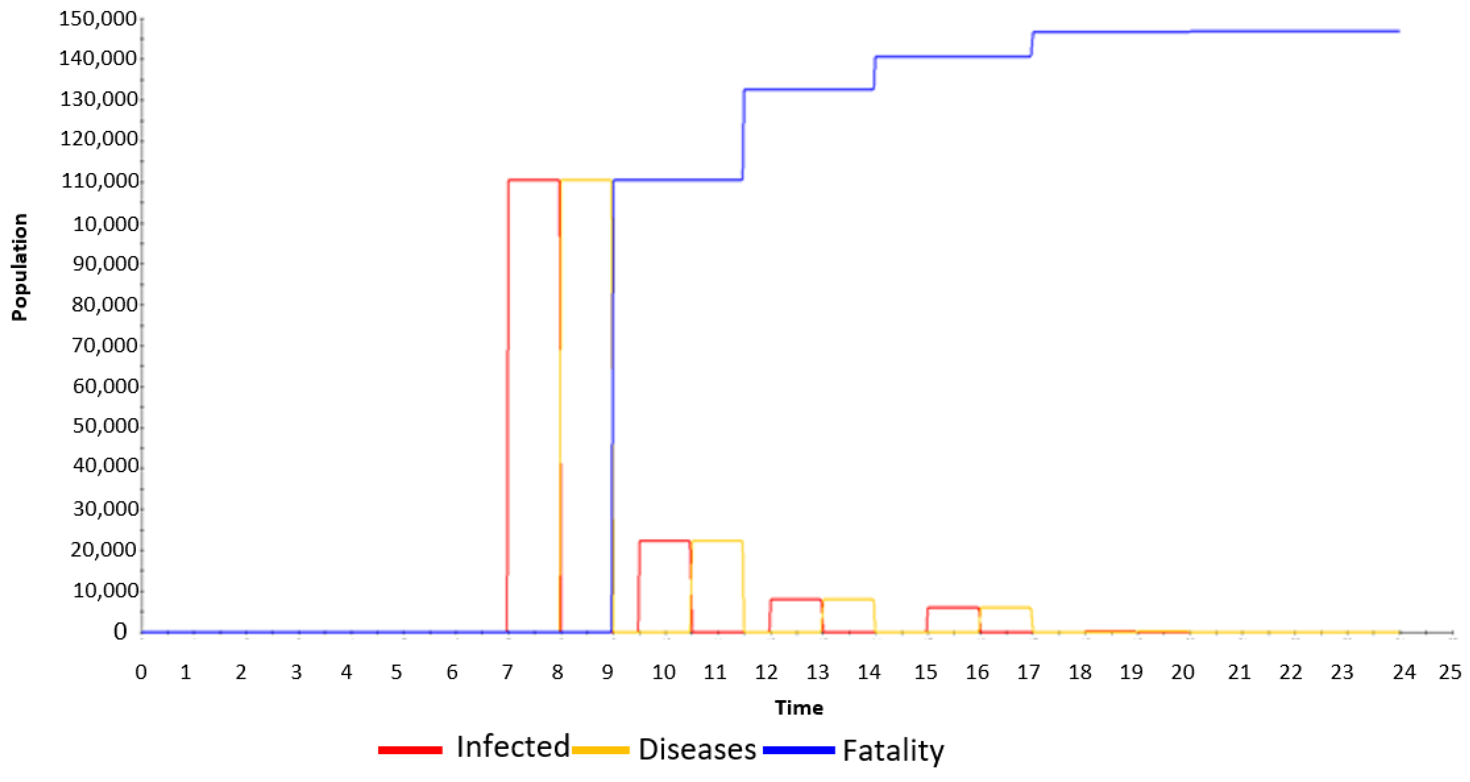
The first case (Loc. 6, Figure 6) has a contaminant that occurs at the source of the water, which means that the injected node is the reservoir, and this contaminant has a massive impact on the water nodes. From Figure 6, the impact of this contaminant appears at most of the nodes in the network, where the impact denoted by different colors, in which the colors indicate the number of people, has been affected by this contaminant (fatality). The different colors used in the map represent different levels of contaminant impact, in which red represents the high impact with a number of population is close to eight-thousand-and-seventy-nine people (8079 people), and the blue color represents the low impact with a number of people in the range between zero and two-hundred. Another way this impact was shown is in terms of fatalities, infection, and diseased people. These categories of impact were done based on the dose threshold values. If the people receive a dose greater than the threshold value, it is reported to one of these categories based on the dose level received. Figure 7 shows the estimated number of people impacted in these three categories, and it depicts that more than six hours after the contaminant spread in the water network, the impact began to appear in the form of infection in the seventh hour to reach the highest value by affecting more than one-hundred-thousand people. The impact appears as diseases in the next hour, recording the same number of impacted people after eight hours, the actual emergence of the fatality began to appear after nine hours, and it reaches its highest value after 7–10 hours with nearly one-hundred-and-fifty-thousand registered infected people.
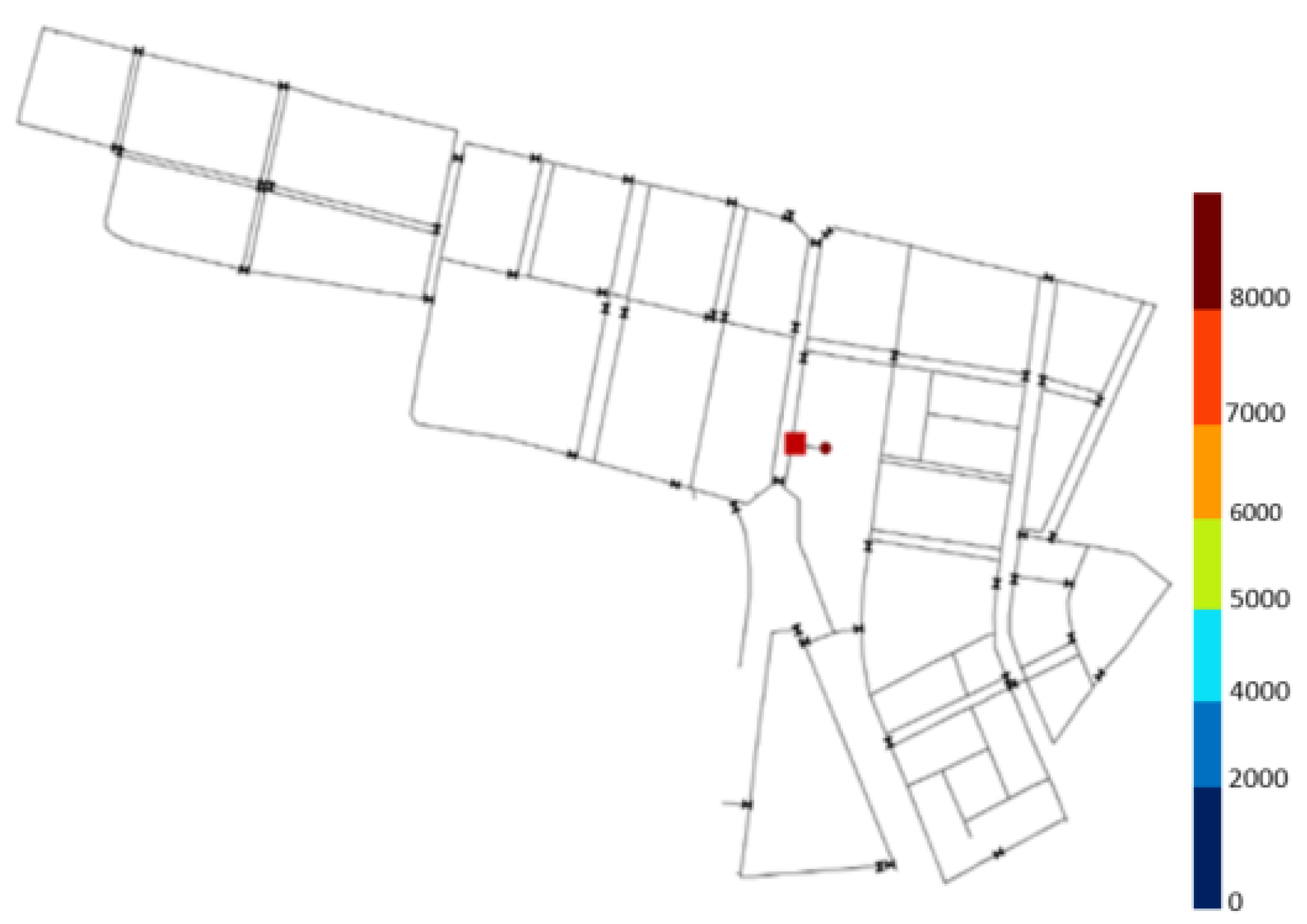
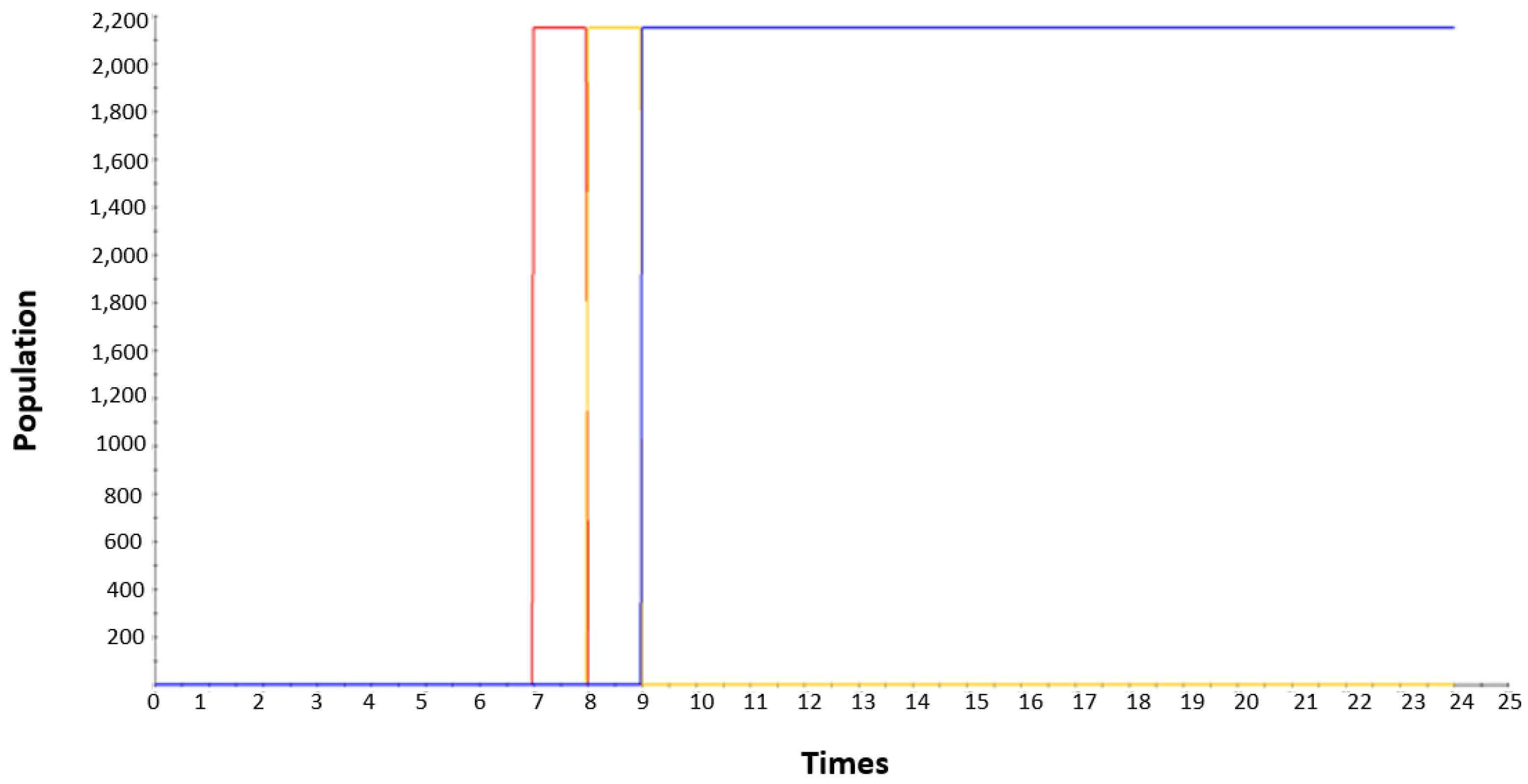
In the second case (Loc. 1), the contaminant occurred in one of the smallest areas of water network (isolated area). Figure 8 shows the special impacts on the node directly related to the contaminated source; the impact is minimal and strictly confined. Comprehensive analysis of the impact of this contaminant source is shown in Figure 9, and we notice that the impact appeared consecutively in the form of infection in the seventh hour, followed by the impact in the way of diseases in the next hour. Finally, the emergence of the fatality rate expected at nine o’clock and the same percentage of impact for people at a rate equal to two-thousand-two-hundred infected people was recorded.
4.2. Reducing the Impact of the Contaminant Using Water Quality Sensors
The main goal of deploying water quality sensors in WDS is to minimize the consequences associated with water contamination. The water quality sensor detects the contaminant based on the contaminant concentration that would change one or more parameters of water quality (i.e., chlorine, TOC, turbidity, and conductivity) enough that an event detection device (sensor) or a water utility operator can detect the change. For instance, if the residual chlorine decreased by 1 mg/L, the conductivity increased by 150 Sm/cm, or the TOC increased by 1 mg/L.
In this section, the impact of water contamination on the lives of consumers is conducted, where the impact of the contaminated water used by people will be recorded before the water quality sensors are deployed. Then, the extent of the contaminant water impact is recorded after the water quality sensors have been deployed based on our proposed approach [30] reviewed in Section 2. Three different numerical experiments have been conducted in this section:
- The first experiment investigated the impact of the contaminant without using water quality sensors.
- The second experiment shows the impact using the water quality sensors optimally deployed on WDS utilizing the volume of the contamination water (VCW) as an objective function for deploying the sensors.
- The third experiment analyzes the impact using water quality sensors that are optimally deployed on WDS using time detection (TD) as an objective function to deploy the sensors.
In the first experiment, the health impact was analyzed without using water quality sensors to detect the water contaminant. Table 3 shows the impact of water contaminant on the people and contains the essential properties to represent the impact of the contaminant, such as the contaminants’ injections nodes, detection time, and the impact as infected people. In Table 3, we have to select thirty injected nodes (as samples) from more than one-thousand nodes included in the Madrid case study, and these samples will be used in all the numerical experiments. As we present this experiment without using deployed sensors (water quality sensors), the detection time is recorded as 1440 min, which means there is no detection until the end of the simulation (24 h). The impact is computed using the proposed model presented in Section 3.2, and it computes the number of people got affected. The impact of the contaminated water without sensors is represented clearly in Figure 10. The x-axis represents the water nodes that are infected with contamination, and the y-axis represents the impact of this contamination concerning the number of people that are affected by this contamination. From Figure 10, we notice that the results were significantly recorded in this experiment, as it was estimated 1that 14,721 cases were recorded at injected node 17_No_1195. At the same time, the rest of the injected water nodes recorded significant numbers of people.
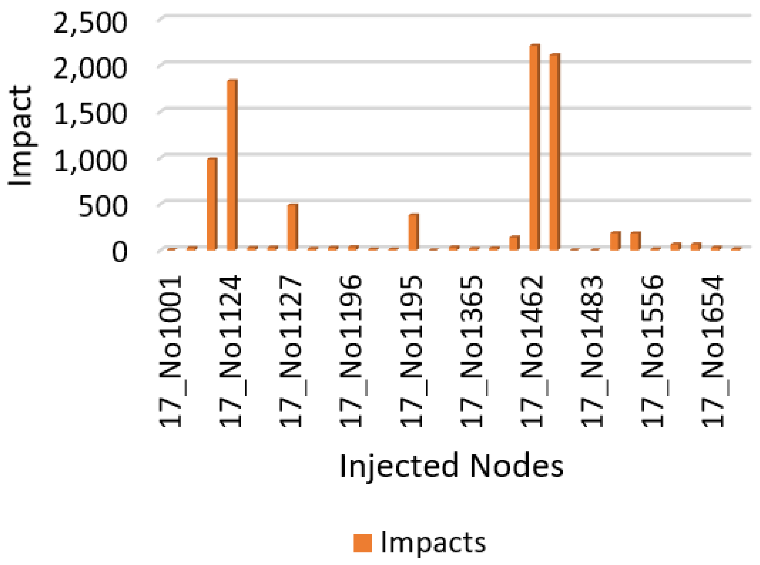
In the second experiment, we have deployed ten sensors as monitoring stations to detect the water contaminant, the deployment of sensors used the volume of contaminant water (VCW) as its optimization objective [30]. Table 4 shows the impact of the contaminant after deploying the ten monitoring sensors, and the table contains the same properties presented in the previous experiment, while the detected stations represent the sensor station that detects the contaminant. The time detection column recorded the detection time of the contaminant by the monitoring stations. From Table 4, despite using monitoring stations (sensors), we still find that some injected nodes are not directly detected by any monitoring stations such as 17_No_1381, 17_No1532, 17_No_1702, and 17_No_1703. These nodes kept the contamination until the end of the simulation (1440 min). The main reason for this is the optimization method used to deploy the sensor in this experiment is still unable to cover all injected nodes. The estimated impact of using ten sensor stations (based on the volume of contaminated consume water) is represented clearly in Figure 11. The x-axis represents the water nodes that are infected with contamination, and the y-axis represents the impact of this contamination concerning the number of people that got impact from this contamination. From Figure 11, we notice that the impact decreased significantly compared to what was presented in the previous experiment. The maximum number of cases recorded in this experiment was estimated at 2211 cases, recorded at injected node 17_No_1462.
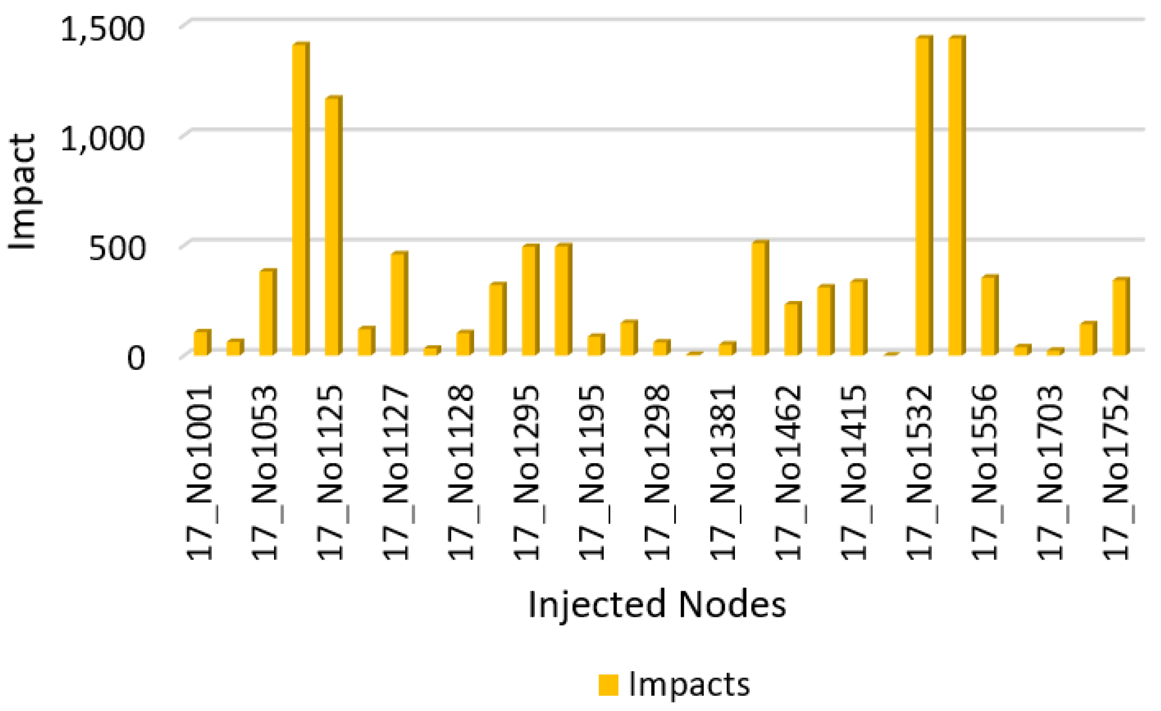
In the third experiment, we deployed ten sensors as monitoring stations to detect water contamination and used time detection (TD) as optimization functions for deployed sensors. Using the same samples used in the previous numerical experiments, Table 5 includes the same properties used in the previous numerical experiments. However, the results show that the number of injected nodes that were not detected by any of the monitor stations (sensors) decreased significantly compared to the previous numerical experiments. Only one injected node (17_No_1532) was not directly covered by any of the monitoring stations, and this injected node recorded the maximum impact of the water contamination. The estimated impacts of pollution are represented clearly in Figure 12. Figure 12 shows the extent of the impact of water pollution, and it has decreased significantly compared to previous experiences in this experiment. The highest number of infected cases was recorded as 1464 cases, recorded at 17_No_1532.
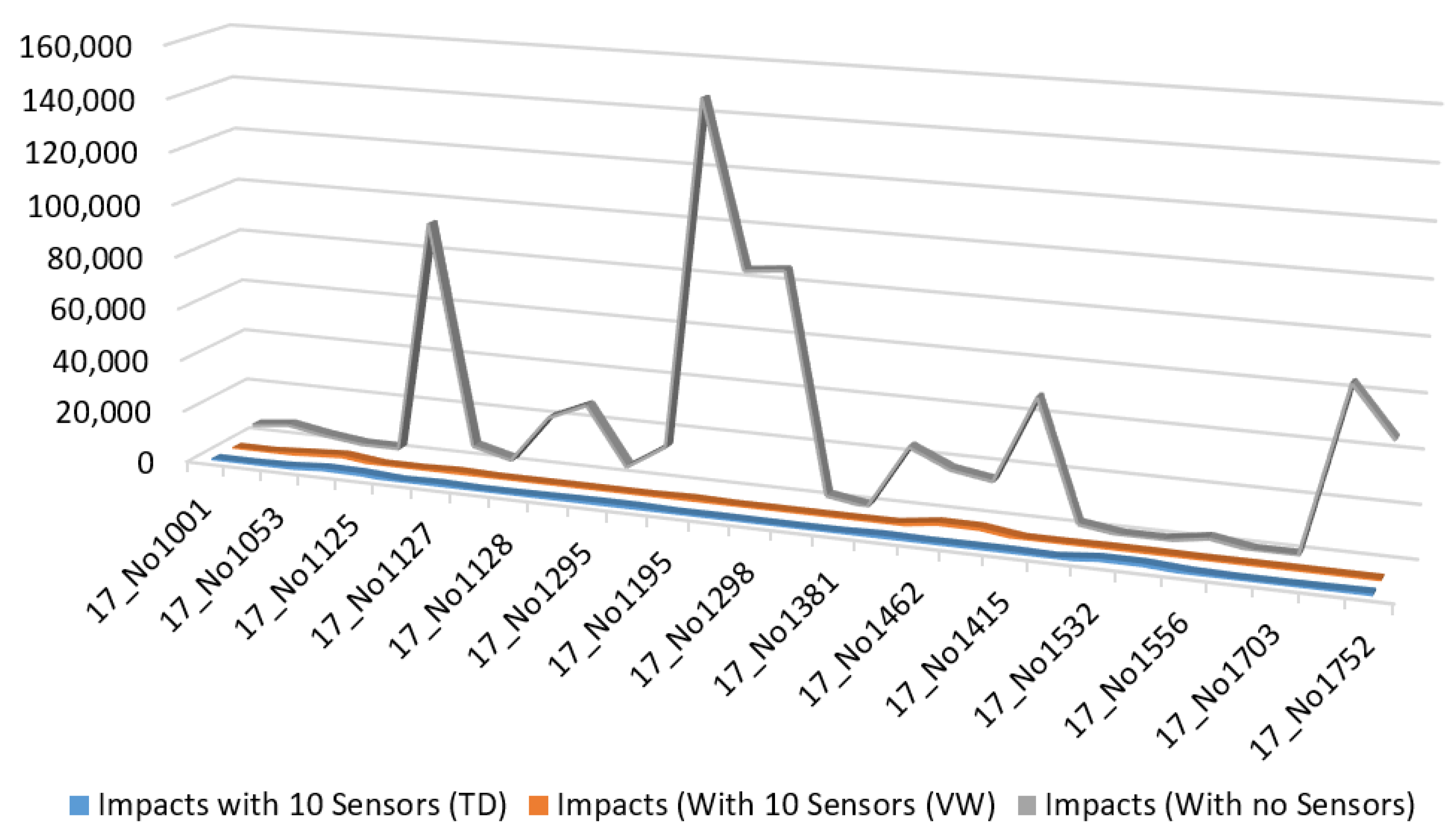
Finally, the comparison of water contaminant impact before deploying the sensors and after the deployment of the sensors is conducted and presented in Figure 13. The results in Figure 13 show a significant impact on the number of people impacted by the contaminant water before the water quality sensors were deployed and recorded a massive amount of more than one-hundred-thousand people. On the other hand, this number decreased with the use of water quality sensors to monitor the quality of the water. These sensors were distributed in the water network based on the previously described method, and different numbers were recorded for the number of people affected by water contaminant. Using the contaminated water volume as an objective function to determine the location of the sensors, the number of people affected was close to two-thousand. On the other hand, the number of people in the situation that time detection is used as a target to locate the sensors is close to one-thousand-and-four-hundred. In summary, the use of water sensors to monitor water quality has shown a big difference in reducing the number of people exposed to the risk of using contaminated water, which shows the effectiveness of the proposed method used to distribute the water quality sensors.
5. Conclusions
In this paper, a health impact analysis model of WDS is proposed to assess and analyze the health impact of consuming contaminated drinking water in a water distributed system (WDS). The health impact analysis process mainly depends on the hydraulic and water quality models in WDS. Water contaminants are injected in various locations and spread in the water network for 8 h before we start the analysis. The health impact for the contaminated scenarios in WDS is examined and simulated using a real case study from a district of Madrid, Spain. The impact of water pollution has been analyzed in different locations with multiple critical threshold values of the dose level. The number of people that were infected, diseased, or died from pollution was recorded in each simulated experiment. Finally, the extent of pollution’s impact was compared without using water quality stations and using ten water quality sensors. These sensors are optimally deployed on WD based on the time detection and volume of the contaminated water. The results showed a very significant reduction in the impact using the deployed sensors, where the health impact was reduced by up to 98.37%.
Author Contributions
Conceptualization E.Q.S. and W.W.; methodology, E.Q.S.; software, E.Q.S. and R.G.; formal analysis, E.Q.S. and W.W.; data, R.G.; writing—original draft preparation, E.Q.S.; writing—review and editing, E.Q.S. and W.W. All authors have read and agreed to the published version of the manuscript
Funding
European Union’s Horizon 2020 research and innovation programme Under the Marie Skłodowska-Curie–Innovative Training Networks (ITN)-IoT4Win-Internet of Things for Smart Water Innovative Network (765921).
Institutional Review Board Statement
Not applicable.
Informed Consent Statement
Not applicable.
Data Availability Statement
The data and the case study used in this article have been provided by TPF Getinsa Eurostudios, Madrid, Spain. These data are not available on the Internet and have been used in this article only.
Acknowledgments
This research is supported by European Union’s Horizon 2020 research and innovation programme Under the Marie Skłodowska-Curie–Innovative Training Networks (ITN)-IoT4Win-Internet of Things for Smart Water Innovative Network (765921).
Conflicts of Interest
The authors declare no conflict of interest.
References
- Li, P.; Wu, J. Drinking water quality and public health. Expo. Health 2019, 11, 73–79. [Google Scholar] [CrossRef]
- Padulano, R.; Del Giudice, G. A nonparametric framework for water consumption data cleansing: An application to a smart water network in Naples (Italy). J. Hydroinform. 2020, 22, 666–680. [Google Scholar] [CrossRef]
- Damiani, M.; Núñez, M.; Roux, P.; Loiseau, E.; Rosenbaum, R.K. Addressing water needs of freshwater ecosystems in life cycle impact assessment of water consumption: State of the art and applicability of ecohydrological approaches to ecosystem quality characterization. Int. J. Life Cycle Assess. 2018, 23, 2071–2088. [Google Scholar] [CrossRef]
- Liu, G.; Zhang, Y.; Knibbe, W.J.; Feng, C.; Liu, W.; Medema, G.; van der Meer, W. Potential impacts of changing supply-water quality on drinking water distribution: A review. Water Res. 2017, 116, 135–148. [Google Scholar] [CrossRef] [PubMed]
- Kara, S.; Karadirek, I.E.; Muhammetoglu, A.; Muhammetoglu, H. Real time monitoring and control in water distribution systems for improving operational efficiency. Desalin. Water Treat. 2016, 57, 11506–11519. [Google Scholar] [CrossRef]
- Frisbie, S.H.; Mitchell, E.J.; Dustin, H.; Maynard, D.M.; Sarkar, B. World Health Organization discontinues its drinking-water guideline for manganese. Environ. Health Perspect. 2012, 120, 775–778. [Google Scholar] [CrossRef] [Green Version]
- Lavoie, R.; Joerin, F.; Rodriguez, M. ATES: A geo-informatics decision aid tool for the integration of groundwater into land planning. J. Hydroinform. 2015, 17, 771–788. [Google Scholar] [CrossRef] [Green Version]
- De Vera, G.A.; Wert, E.C. Using discrete and online ATP measurements to evaluate regrowth potential following ozonation and (non) biological drinking water treatment. Water Res. 2019, 154, 377–386. [Google Scholar] [CrossRef]
- Long, D.T.; Pearson, A.L.; Voice, T.C.; Polanco-Rodríguez, A.G.; Sanchez-Rodríguez, E.C.; Xagoraraki, I.; Concha-Valdez, F.G.; Puc-Franco, M.; Lopez-Cetz, R.; Rzotkiewicz, A.T. Influence of rainy season and land use on drinking water quality in a karst landscape, State of Yucatán, Mexico. Appl. Geochem. 2018, 98, 265–277. [Google Scholar] [CrossRef]
- Scheili, A.; Rodriguez, M.; Sadiq, R. Seasonal and spatial variations of source and drinking water quality in small municipal systems of two Canadian regions. Sci. Total Environ. 2015, 508, 514–524. [Google Scholar] [CrossRef]
- Abtahi, M.; Golchinpour, N.; Yaghmaeian, K.; Rafiee, M.; Jahangiri-rad, M.; Keyani, A.; Saeedi, R. A modified drinking water quality index (DWQI) for assessing drinking source water quality in rural communities of Khuzestan Province, Iran. Ecol. Indic. 2015, 53, 283–291. [Google Scholar] [CrossRef]
- Rodriguez-Narvaez, O.M.; Peralta-Hernandez, J.M.; Goonetilleke, A.; Bandala, E.R. Treatment technologies for emerging contaminants in water: A review. Chem. Eng. J. 2017, 323, 361–380. [Google Scholar] [CrossRef] [Green Version]
- Chang, K.; Gao, J.L.; Wu, W.Y.; Yuan, Y.X. Water quality comprehensive evaluation method for large water distribution network based on clustering analysis. J. Hydroinform. 2011, 13, 390–400. [Google Scholar] [CrossRef]
- Soltani, A.A.; Oukil, A.; Boutaghane, H.; Bermad, A.; Boulassel, M.R. A new methodology for assessing water quality, based on data envelopment analysis: Application to Algerian dams. Ecol. Indic. 2021, 121, 106952. [Google Scholar] [CrossRef]
- Baştürk, E. Assessing Water Quality of Mamasın Dam, Turkey: Using Water Quality Index Method, Ecological and Health Risk Assessments. CLEAN-Air Water 2019, 47, 1900251. [Google Scholar] [CrossRef]
- Wu, Z.; Zhang, D.; Cai, Y.; Wang, X.; Zhang, L.; Chen, Y. Water quality assessment based on the water quality index method in Lake Poyang: The largest freshwater lake in China. Sci. Rep. 2017, 7, 1–10. [Google Scholar] [CrossRef]
- Abtahi, M.; Yaghmaeian, K.; Mohebbi, M.R.; Koulivand, A.; Rafiee, M.; Jahangiri-rad, M.; Jorfi, S.; Saeedi, R.; Oktaie, S. An innovative drinking water nutritional quality index (DWNQI) for assessing drinking water contribution to intakes of dietary elements: A national and sub-national study in Iran. Ecol. Indic. 2016, 60, 367–376. [Google Scholar] [CrossRef]
- Akter, T.; Jhohura, F.T.; Akter, F.; Chowdhury, T.R.; Mistry, S.K.; Dey, D.; Barua, M.K.; Islam, M.A.; Rahman, M. Water Quality Index for measuring drinking water quality in rural Bangladesh: A cross-sectional study. J. Health Popul. Nutr. 2016, 35, 1–12. [Google Scholar] [CrossRef] [Green Version]
- Ba, A.; McKenna, S.A. Water quality monitoring with online change-point detection methods. J. Hydroinform. 2015, 17, 7–19. [Google Scholar] [CrossRef]
- Braun, M.; Piller, O.; Deuerlein, J.; Mortazavi, I.; Iollo, A. Uncertainty quantification of water age in water supply systems by use of spectral propagation. J. Hydroinform. 2020, 22, 111–120. [Google Scholar] [CrossRef]
- Banda, T.D.; Kumarasamy, M.V. Development of Water Quality Indices (WQIs): A Review. Pol. J. Environ. Stud. 2020, 29. [Google Scholar] [CrossRef]
- Gara, T.; Fengting, L.; Nhapi, I.; Makate, C.; Gumindoga, W. Health safety of drinking water supplied in Africa: A closer look using applicable water-quality standards as a measure. Expo. Health 2018, 10, 117–128. [Google Scholar] [CrossRef]
- Chen, J.; Qian, H.; Gao, Y.; Li, X. Human health risk assessment of contaminants in drinking water based on triangular fuzzy numbers approach in Yinchuan City, Northwest China. Expo. Health 2018, 10, 155–166. [Google Scholar] [CrossRef]
- Zhang, H.; Zhou, X.; Wang, L.; Wang, W.; Xu, J. Concentrations and potential health risks of strontium in drinking water from Xi’an, Northwest China. Ecotoxicol. Environ. Saf. 2018, 164, 181–188. [Google Scholar] [CrossRef] [PubMed]
- Ali, N.; Khan, S.; ur Rahman, I.; Muhammad, S. Human health risk assessment through consumption of organophosphate pesticide-contaminated water of Peshawar basin, Pakistan. Expo. Health 2018, 10, 259–272. [Google Scholar] [CrossRef]
- Joshi, Y.P.; Kim, J.H.; Kim, H.; Cheong, H.K. Impact of drinking water quality on the development of enteroviral diseases in Korea. Int. J. Environ. Res. Public Health 2018, 15, 2551. [Google Scholar] [CrossRef] [Green Version]
- Zhang, Q.; Xu, P.; Qian, H. Groundwater quality assessment using improved water quality index (WQI) and human health risk (HHR) evaluation in a semi-arid region of northwest China. Expo. Health 2020, 12, 487–500. [Google Scholar] [CrossRef]
- Adimalla, N.; Li, P. Occurrence, health risks, and geochemical mechanisms of fluoride and nitrate in groundwater of the rock-dominant semi-arid region, Telangana State, India. Hum. Ecol. Risk Assess. Int. J. 2019, 25, 81–103. [Google Scholar] [CrossRef]
- Kumar, D.; Singh, A.; Jha, R.K.; Sahoo, S.K.; Jha, V. A variance decomposition approach for risk assessment of groundwater quality. Expo. Health 2019, 11, 139–151. [Google Scholar] [CrossRef]
- Shahra, E.Q.; Wu, W. Water contaminants detection using sensor placement approach in smart water networks. J. Ambient. Intell. Humaniz. Comput. 2020, 1–16. [Google Scholar] [CrossRef]
- Ung, H.; Piller, O.; Gilbert, D.; Mortazavi, I. Accurate and optimal sensor placement for source identification of water distribution networks. J. Water Resour. Plan. Manag. 2017, 143, 04017032. [Google Scholar] [CrossRef] [Green Version]
- Hooshmand, F.; Amerehi, F.; MirHassani, S. Risk-Based Models for Optimal Sensor Location Problems in Water Networks. J. Water Resour. Plan. Manag. 2020, 146, 04020086. [Google Scholar] [CrossRef]
- Santonastaso, G.F.; Di Nardo, A.; Creaco, E.; Musmarra, D.; Greco, R. Comparison of topological, empirical and optimization-based approaches for locating quality detection points in water distribution networks. Environ. Sci. Pollut. Res. 2020, 1–10. [Google Scholar] [CrossRef]
- Hu, C.; Yan, X.; Gong, W.; Liu, X.; Wang, L.; Gao, L. Multi-objective based scheduling algorithm for sudden drinking water contamination incident. Swarm Evol. Comput. 2020, 55, 100674. [Google Scholar] [CrossRef]
- Janke, R.; Murray, R.; Haxton, T.; Taxon, T.; Bahadur, R.; Samuels, W.; Berry, J.; Boman, E.; Hart, W.; Riesen, L.; et al. Threat Ensemble Vulnerability Assessment-Sensor Placement Optimization Tool (TEVA-SPOT) Graphical User Interface User’S Manual; Researchgate: Berlin, Germany, 2012; pp. 1–109. [Google Scholar]
- Bałut, A.; Urbaniak, A. Application of the TEVA-SPOT in designing the monitoring of water networks. E3S Web Conf. EDP Sci. 2018, 59, 00009. [Google Scholar] [CrossRef] [Green Version]
- Davis, M.J.; Janke, R.; Taxon, T.N. Mass imbalances in EPANET water-quality simulations. Drink. Water Eng. Sci. 2018, 11, 25–47. [Google Scholar] [CrossRef] [PubMed] [Green Version]
- Studziński, A.; Pietrucha-Urbanik, K. Simulation model of contamination threat assessment in water network using the EPANET software. Ecol. Chem. Eng. S 2016, 23, 425–433. [Google Scholar] [CrossRef] [Green Version]
- Davis, M.J.; Janke, R.; Magnuson, M.L. A framework for estimating the adverse health effects of contamination events in water distribution systems and its application. Risk Anal. 2014, 34, 498–513. [Google Scholar] [CrossRef]
Figure 1.
Water distributed networks from Madrid (city center).

Figure 2.
The proposed model of health analysis

Figure 3.
The concentration of the contaminant after 8 h for the injected node (reservoir).

Figure 4.
Population distribution based on water demand.

Figure 5.
Areas of the contaminant locations.

Figure 6.
Estimated impact for contaminant occurred at water source (Reservoir).

Figure 7.
Estimated infection, disease, and fatalities (contamination at source).

Figure 8.
Estimated impact for contaminant at one of the small isolated networks.

Figure 9.
Estimated infection, disease, and fatalities (contaminant at the isolated branch).

Figure 10.
Health impact without using water quality sensors.

Figure 11.
Health impact with 10 sensors deployed using volume of contaminated water (VCW).

Figure 12.
Health impact with 10 sensors deployed using time detection (TD).

Figure 13.
Comparison of the health impact for three scenarios.


Table 1.
Water contaminant parameters.
| Parameters | Values |
|---|---|
| Contaminant type | Chemical/Toxin |
| Average Body Mass (KG) | 70.0 |
| Water Ingestion Rate (Liters per day) | 1.41 |
| Gallons per Person per Day (GPD) | 200 |
| LD50 (mg/kg) | 0.001 |
| Simulation Start time | 00:00 A.M. |
| Simulation Length | 24 h |
| Injection Start Time | 00:00 A.M. |
| Injection Duration | 8 h |
| Injection Node | Reservoir |
Table 2.
Infected people based on contamination locations.
| Contamination Locations | Maximum Concentration (Mg/L) | Maximum Individual Dose (mg) | Number of Estimated Infected People |
|---|---|---|---|
| Loc. 1 | 2993 | 1 | 0 |
| Loc. 2 | 30 | 2 | 2750 |
| Loc. 3 | 44 | 5 | 7217 |
| Loc. 4 | 224 | 11 | 29,017 |
| Loc. 5 | 27 | 16 | 43,996 |
| Loc. 6 | 2 | 91 | 146,729 |
| Mean | 217 | 8 | 18,568 |
Table 3.
Health impact without using any water quality monitor stations.
| Injection Nodes in WDS | Detection Time (Minutes) | Infected People |
|---|---|---|
| 17_No1001 | 1440 | 4858 |
| 17_No1002 | 1440 | 6499 |
| 17_No1053 | 1440 | 3899 |
| 17_No1124 | 1440 | 2071 |
| 17_No1125 | 1440 | 2042 |
| 17_No1113 | 1440 | 91,710 |
| 17_No1127 | 1440 | 6364 |
| 17_No1126 | 1440 | 2512 |
| 17_No1128 | 1440 | 20,742 |
| 17_No1196 | 1440 | 27,215 |
| 17_No1295 | 1440 | 4821 |
| 17_No1296 | 1440 | 14,360 |
| 17_No1195 | 1440 | 114,721 |
| 17_No1297 | 1440 | 84,217 |
| 17_No1298 | 1440 | 85,784 |
| 17_No1365 | 1440 | 2492 |
| 17_No1381 | 1440 | 23 |
| 17_No1414 | 1440 | 24,377 |
| 17_No1462 | 1440 | 17,485 |
| 17_No1463 | 1440 | 14,949 |
| 17_No1415 | 1440 | 47,880 |
| 17_No1483 | 1440 | 2493 |
| 17_No1532 | 1440 | 186 |
| 17_No1533 | 1440 | 183 |
| 17_No1556 | 1440 | 2666 |
| 17_No1702 | 1440 | 64 |
| 17_No1703 | 1440 | 64 |
| 17_No1654 | 1440 | 63,882 |
| 17_No1752 | 1440 | 45,190 |
Table 4.
Health impact with using 10 water quality sensors using (VCW).
| Injection Nodes in WDS | Detection Sensors | Detection Time | Infected People |
|---|---|---|---|
| 17_No1001 | 17_No1891 | 106 | 3 |
| 17_No1002 | 17_No1891 | 66 | 24 |
| 17_No1053 | 17_No1483 | 382 | 982 |
| 17_No1124 | 17_No1483 | 1410 | 1829 |
| 17_No1125 | 17_No1483 | 1166 | 25 |
| 17_No1113 | 17_No1297 | 8 | 30 |
| 17_No1127 | 17_No525 | 612 | 485 |
| 17_No1126 | 17_No1483 | 32 | 16 |
| 17_No1128 | 17_No3856 | 104 | 28 |
| 17_No1196 | 17_No3707 | 24 | 35 |
| 17_No1295 | 17_No525 | 494 | 10 |
| 17_No1296 | 17_No525 | 496 | 10 |
| 17_No1195 | 17_No3707 | 26 | 378 |
| 17_No1297 | 17_No1297 | 0 | 0 |
| 17_No1298 | 17_No1415 | 48 | 32 |
| 17_No1365 | 17_No1483 | 4 | 17 |
| 17_No1381 | 1440 | 23 | |
| 17_No1414 | 17_No3856 | 512 | 140 |
| 17_No1462 | 17_No4702 | 232 | 2211 |
| 17_No1463 | 17_No2087 | 310 | 2111 |
| 17_No1415 | 17_No1415 | 0 | 0 |
| 17_No1483 | 17_No1483 | 0 | 0 |
| 17_No1532 | 1440 | 186 | |
| 17_No1533 | 1440 | 183 | |
| 17_No1556 | 17_No1483 | 354 | 11 |
| 17_No1702 | 1440 | 64 | |
| 17_No1703 | 1440 | 64 | |
| 17_No1654 | 17_No1415 | 54 | 29 |
| 17_No1752 | 17_No1483 | 342 | 12 |
Table 5.
Health impact with using 10 water quality sensors using time detection (TD).
| Injection Nodes in WDS | Detection Sensors | Detection Time | Infected People (People) |
|---|---|---|---|
| 17_No1001 | 17_No1891 | 106 | 108 |
| 17_No1002 | 17_No2830 | 62 | 65 |
| 17_No1053 | 17_No1483 | 382 | 386 |
| 17_No1124 | 17_No1483 | 1410 | 1415 |
| 17_No1125 | 17_No1483 | 1166 | 1172 |
| 17_No1113 | 17_No5633 | 120 | 127 |
| 17_No1127 | 17_No4089 | 460 | 468 |
| 17_No1126 | 17_No1483 | 32 | 41 |
| 17_No1128 | 17_No4089 | 102 | 112 |
| 17_No1196 | 17_No525 | 320 | 331 |
| 17_No1295 | 17_No525 | 494 | 506 |
| 17_No1296 | 17_No525 | 496 | 509 |
| 17_No1195 | 17_No525 | 86 | 100 |
| 17_No1297 | 17_No5633 | 148 | 163 |
| 17_No1298 | 17_No5633 | 60 | 76 |
| 17_No1365 | 17_No1483 | 4 | 21 |
| 17_No1381 | 17_No348 | 50 | 68 |
| 17_No1414 | 17_No4089 | 510 | 529 |
| 17_No1462 | 17_No4702 | 232 | 252 |
| 17_No1463 | 17_No2087 | 310 | 331 |
| 17_No1415 | 17_No1483 | 334 | 356 |
| 17_No1483 | 17_No1483 | 2 | 23 |
| 17_No1532 | 1440 | 1464 | |
| 17_No1533 | 17_No1483 | 1200 | 1225 |
| 17_No1556 | 17_No_1483 | 354 | 380 |
| 17_No1702 | 17_No961 | 38 | 65 |
| 17_No1703 | 17_No961 | 22 | 50 |
| 17_No1654 | 17_No1483 | 142 | 171 |
| 17_No1752 | 17_No1483 | 342 | 372 |
Publisher’s Note: MDPI stays neutral with regard to jurisdictional claims in published maps and institutional affiliations. |
© 2021 by the authors. Licensee MDPI, Basel, Switzerland. This article is an open access article distributed under the terms and conditions of the Creative Commons Attribution (CC BY) license (https://creativecommons.org/licenses/by/4.0/).
Share and Cite
MDPI and ACS Style
Shahra, E.Q.; Wu, W.; Gomez, R. Human Health Impact Analysis of Contaminant in IoT-Enabled Water Distributed Networks. Appl. Sci. 2021, 11, 3394. https://0-doi-org.brum.beds.ac.uk/10.3390/app11083394
AMA Style
Shahra EQ, Wu W, Gomez R. Human Health Impact Analysis of Contaminant in IoT-Enabled Water Distributed Networks. Applied Sciences. 2021; 11(8):3394. https://0-doi-org.brum.beds.ac.uk/10.3390/app11083394
Chicago/Turabian StyleShahra, Essa Q., Wenyan Wu, and Roberto Gomez. 2021. "Human Health Impact Analysis of Contaminant in IoT-Enabled Water Distributed Networks" Applied Sciences 11, no. 8: 3394. https://0-doi-org.brum.beds.ac.uk/10.3390/app11083394
Note that from the first issue of 2016, this journal uses article numbers instead of page numbers. See further details here.